Title stata.com

intro 5 — Tour of models

Description Remarks and examples References Also see

DescriptionBelow is a sampling of SEMs that can be fit by sem or gsem.

Remarks and examples stata.com

If you have not read [SEM] intro 2, please do so. You need to speak the language. We alsorecommend reading [SEM] intro 4, but that is not required.

Now that you speak the language, we can start all over again and take a look at some of theclassic models that sem and gsem can fit.

Remarks are presented under the following headings:

Single-factor measurement modelsItem–response theory (IRT) modelsMultiple-factor measurement modelsConfirmatory factor analysis (CFA) modelsStructural models 1: Linear regressionStructural models 2: Gamma regressionStructural models 3: Binary-outcome modelsStructural models 4: Count modelsStructural models 5: Ordinal modelsStructural models 6: Multinomial logistic regressionStructural models 7: Dependencies between response variablesStructural models 8: Unobserved inputs, outputs, or bothStructural models 9: MIMIC modelsStructural models 10: Seemingly unrelated regression (SUR)Structural models 11: Multivariate regressionStructural models 12: Mediation modelsCorrelationsHigher-order CFA modelsCorrelated uniqueness modelLatent growth modelsModels with reliabilityMultilevel mixed-effects models

1

2 intro 5 — Tour of models

Single-factor measurement models

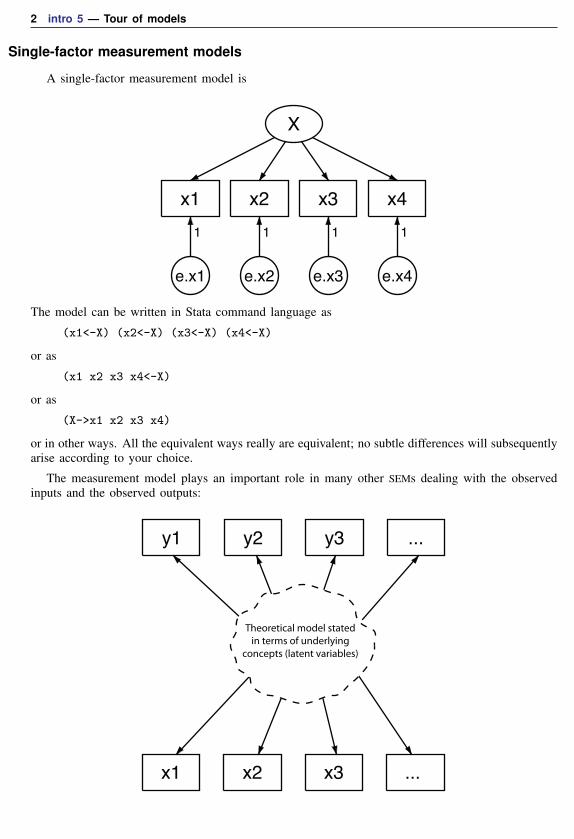
A single-factor measurement model is

X

x1

e.x1

1

x2

e.x2

1

x3

e.x3

1

x4

e.x4

1

The model can be written in Stata command language as

(x1<-X) (x2<-X) (x3<-X) (x4<-X)

or as

(x1 x2 x3 x4<-X)

or as

(X->x1 x2 x3 x4)

or in other ways. All the equivalent ways really are equivalent; no subtle differences will subsequentlyarise according to your choice.

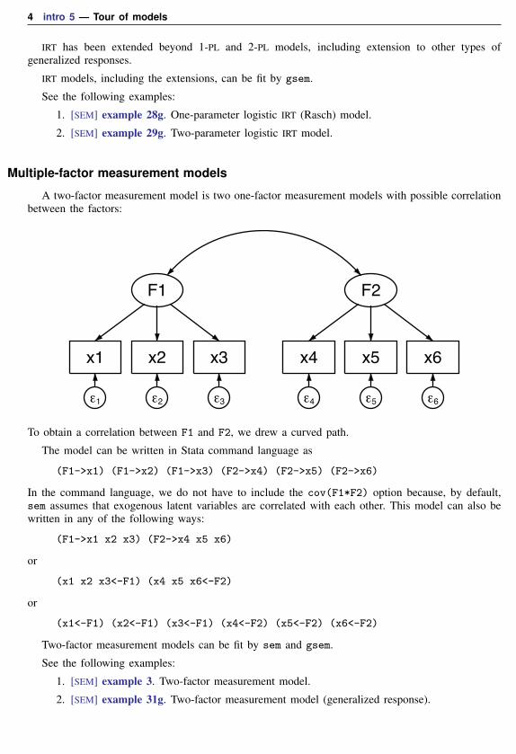
The measurement model plays an important role in many other SEMs dealing with the observedinputs and the observed outputs:

y1 y2 y3 ...

x1 x2 x3 ...

Theoretical model stated

in terms of underlying

concepts (latent variables)

intro 5 — Tour of models 3

Because the measurement model is so often joined with other models, it is common to refer to thecoefficients on the paths from latent variables to observable endogenous variables as the measurementcoefficients and to refer to their intercepts as the measurement intercepts. The intercepts are usually notshown in path diagrams. The other coefficients and intercepts are those not related to the measurementissue.

The measurement coefficients are often referred to as loadings.

This model can be fit by sem or gsem. Use sem for standard linear models (standard meanssingle level); use gsem when you are fitting a multilevel model or when the response variables aregeneralized linear such as probit, logit, multinomial logit, Poisson, and so on.

See the following examples:

1. [SEM] example 1. Single-factor measurement model.

2. [SEM] example 27g. Single-factor measurement model (generalized response).

3. [SEM] example 30g. Two-level measurement model (multilevel, generalized response).

4. [SEM] example 35g. Ordered probit and ordered logit.

Item–response theory (IRT) models

Item–response theory (IRT) models look like the following:

L

item1

Bernoulli

logit

item2

Bernoulli

logit

item3

Bernoulli

logit

item4

Bernoulli

logit

The items are the observed variables, and each has a 0/1 outcome measuring a latent variable. Often,the latent variable represents ability. These days, it is traditional to fit IRT models using logisticregression, but in the past, probit was used and they were called normal ogive models.

In one-parameter logistic models, also known as 1-PL models and Rasch models, constraintsare placed on the paths and perhaps the variance of the latent variable. Either path coefficients areconstrained to 1 or path coefficients are constrained to be equal and the variance of the latent variableis constrained to be 1. Either way, this results in the negative of the intercepts of the fitted modelbeing a measure of difficulty.

1-PL and Rasch models can be fit treating the latent variable—ability—as either fixed or random.Abilities are treated as random with gsem.

In two-parameter logistic models (2-PL), no constraints are imposed beyond the one required toidentify the latent variable, which is usually done by constraining the variance to 1. This resultsin path coefficients measuring discriminating ability of the items, and difficulty is measured by thenegative of the intercepts divided by the corresponding (slope) coefficient.

4 intro 5 — Tour of models

IRT has been extended beyond 1-PL and 2-PL models, including extension to other types ofgeneralized responses.

IRT models, including the extensions, can be fit by gsem.

See the following examples:

1. [SEM] example 28g. One-parameter logistic IRT (Rasch) model.

2. [SEM] example 29g. Two-parameter logistic IRT model.

Multiple-factor measurement models

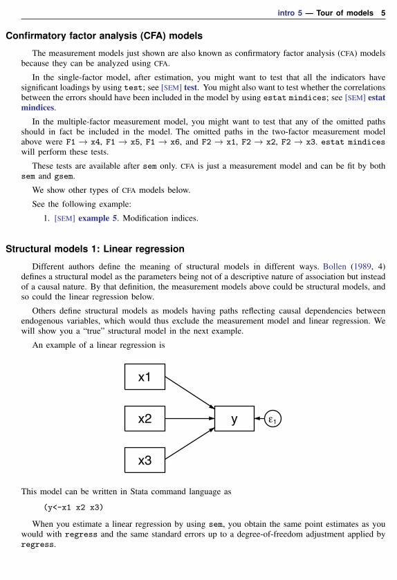
A two-factor measurement model is two one-factor measurement models with possible correlationbetween the factors:

F1

x1

ε1

x2

ε2

x3

ε3

F2

x4

ε4

x5

ε5

x6

ε6

To obtain a correlation between F1 and F2, we drew a curved path.

The model can be written in Stata command language as

(F1->x1) (F1->x2) (F1->x3) (F2->x4) (F2->x5) (F2->x6)

In the command language, we do not have to include the cov(F1*F2) option because, by default,sem assumes that exogenous latent variables are correlated with each other. This model can also bewritten in any of the following ways:

(F1->x1 x2 x3) (F2->x4 x5 x6)

or

(x1 x2 x3<-F1) (x4 x5 x6<-F2)

or

(x1<-F1) (x2<-F1) (x3<-F1) (x4<-F2) (x5<-F2) (x6<-F2)

Two-factor measurement models can be fit by sem and gsem.

See the following examples:

1. [SEM] example 3. Two-factor measurement model.

2. [SEM] example 31g. Two-factor measurement model (generalized response).

intro 5 — Tour of models 5

Confirmatory factor analysis (CFA) models

The measurement models just shown are also known as confirmatory factor analysis (CFA) modelsbecause they can be analyzed using CFA.

In the single-factor model, after estimation, you might want to test that all the indicators havesignificant loadings by using test; see [SEM] test. You might also want to test whether the correlationsbetween the errors should have been included in the model by using estat mindices; see [SEM] estatmindices.

In the multiple-factor measurement model, you might want to test that any of the omitted pathsshould in fact be included in the model. The omitted paths in the two-factor measurement modelabove were F1 → x4, F1 → x5, F1 → x6, and F2 → x1, F2 → x2, F2 → x3. estat mindiceswill perform these tests.

These tests are available after sem only. CFA is just a measurement model and can be fit by bothsem and gsem.

We show other types of CFA models below.

See the following example:

1. [SEM] example 5. Modification indices.

Structural models 1: Linear regression

Different authors define the meaning of structural models in different ways. Bollen (1989, 4)defines a structural model as the parameters being not of a descriptive nature of association but insteadof a causal nature. By that definition, the measurement models above could be structural models, andso could the linear regression below.

Others define structural models as models having paths reflecting causal dependencies betweenendogenous variables, which would thus exclude the measurement model and linear regression. Wewill show you a “true” structural model in the next example.

An example of a linear regression is

y ε1

x1

x2

x3

This model can be written in Stata command language as

(y<-x1 x2 x3)

When you estimate a linear regression by using sem, you obtain the same point estimates as youwould with regress and the same standard errors up to a degree-of-freedom adjustment applied byregress.

6 intro 5 — Tour of models

Linear regression models can be fit by sem and gsem. gsem also has options for censoring.

See the following examples:

1. [SEM] example 6. Linear regression.

2. [SEM] example 38g. Random-intercept and random-slope models (multilevel).

3. [SEM] example 40g. Crossed models (multilevel).

4. [SEM] example 43g. Tobit regression.

5. [SEM] example 44g. Interval regression.

Structural models 2: Gamma regression

Gamma regression, also known as log-Gamma regression, is used when a continuous outcomeis nonnegative, when it ranges from zero to infinity, and often with positively skewed data. It isappropriate when the error variance can be assumed to increase with the mean. Gamma regressiongives similar results to linear regression with a logged dependent variable.

y

gamma

log

x1

x2

x3

Gamma regression is fit by gsem; specify shorthand gamma or specify family(gamma) link(log).

You can fit exponential regressions using Gamma regression if you constrain the log of the scaleparameter to be 0; see [SEM] gsem family-and-link options.

Structural models 3: Binary-outcome models

Binary-outcome models have 0/1 response variables. These models include logistic regression (alsoknown as logit), probit, and complementary log-log (also known as cloglog) models.

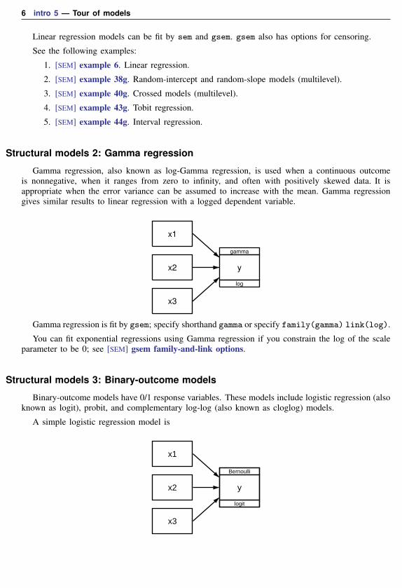
A simple logistic regression model is

y

Bernoulli

logit

x1

x2

x3

intro 5 — Tour of models 7

which in command syntax can be written as

(y<-x1 x2 x3, logit)

For the other binary-outcome models, all that changes in the diagram is the names of the family andlink; in the command language, the option name changes; see [SEM] gsem family-and-link options.

Usually, the observations in binary-outcome data record whether the event occurred, but the datacan instead record the number of events and the number of trials by changing the family fromBernoulli to binomial; see [SEM] gsem family-and-link options.

Binary-outcome models can be fit by gsem.

See the following examples:

1. [SEM] example 33g. Logistic regression.

2. [SEM] example 27g. Single-factor measurement model (generalized response).

3. [SEM] example 34g. Combined models (generalized responses).

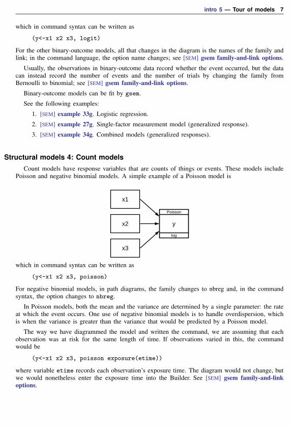
Structural models 4: Count modelsCount models have response variables that are counts of things or events. These models include

Poisson and negative binomial models. A simple example of a Poisson model is

y

Poisson

log

x1

x2

x3

which in command syntax can be written as

(y<-x1 x2 x3, poisson)

For negative binomial models, in path diagrams, the family changes to nbreg and, in the commandsyntax, the option changes to nbreg.

In Poisson models, both the mean and the variance are determined by a single parameter: the rateat which the event occurs. One use of negative binomial models is to handle overdispersion, whichis when the variance is greater than the variance that would be predicted by a Poisson model.

The way we have diagrammed the model and written the command, we are assuming that eachobservation was at risk for the same length of time. If observations varied in this, the commandwould be

(y<-x1 x2 x3, poisson exposure(etime))

where variable etime records each observation’s exposure time. The diagram would not change, butwe would nonetheless enter the exposure time into the Builder. See [SEM] gsem family-and-linkoptions.

8 intro 5 — Tour of models

Count models are fit by gsem.

See the following examples:

1. [SEM] example 34g. Combined models (generalized responses).

2. [SEM] example 39g. Three-level model (multilevel, generalized response).

Structural models 5: Ordinal models

Ordinal models have two or more possible outcomes that are ordered, such as responses of theform “a little”, “average”, and “a lot”; or “strongly disagree”, “disagree”, . . . , “strongly agree”. Theoutcomes are usually numbered 1, 2, . . . , k. These models include ordered probit, ordered logit, andordered complementary log-log (also known as ordered cloglog). A simple example of an orderedprobit model is

y

ordinal

probit

x1

x2

x3

which in command syntax can be written as

(y<-x1 x2 x3, oprobit)

All that changes for the other models is the link name that appears in the path diagram or the optionthat appears in the command language.

Ordinal models are fit by gsem.

See the following examples:

1. [SEM] example 35g. Ordered probit and ordered logit.

2. [SEM] example 31g. Two-factor measurement model (generalized response).

3. [SEM] example 32g. Full structural equation model (generalized response).

4. [SEM] example 36g. MIMIC model (generalized response).

Structural models 6: Multinomial logistic regression

Multinomial logistic regression, also known as multinomial logit, is similar to ordinal models inthat it, too, deals with multiple responses; however, in multinomial logistic regression, the responsescannot be ordered. Examples of multinomial logit response include method of transportation (car,public transportation, etc.) or ice-cream flavor (vanilla, chocolate, etc.).

Just as with ordinal models, the outcome is usually recorded as a single variable containing 1, 2,. . . , k, but in path diagrams, factor-variable notation is used to identify the outcomes:

intro 5 — Tour of models 9

1b.y

multinomial

logit

2.y

multinomial

logit

3.y

multinomial

logit

x1

x2

In command syntax, this can be written as

(i.y<-x1 x2, mlogit)

In the example above, we have paths from all predictor variables to all outcomes. That is commonbut not required.

The multinomial logistic regression model is fit by gsem.

See the following examples:

1. [SEM] example 37g. Multinomial logistic regression.

2. [SEM] example 41g. Two-level multinomial logistic regression (multilevel).

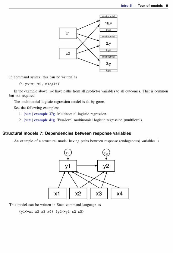
Structural models 7: Dependencies between response variables

An example of a structural model having paths between response (endogenous) variables is

x1 x2 x3 x4

y1

ε1

y2

ε2

This model can be written in Stata command language as

(y1<-x1 x2 x3 x4) (y2<-y1 x2 x3)

10 intro 5 — Tour of models

In this example, all inputs and outputs are observed and the errors are assumed to be uncorrelated.In these kinds of models, it is common to allow correlation between errors:

x1 x2 x3 x4

y1

ε1

y2

ε2

The model above can be written in Stata command language as

(y1<-x1 x2 x3 x4) (y2<-y1 x2 x3), cov(e.y1*e.y2)

This structural model is said to be overidentified. If we omitted y1 ← x4, the model would bejust-identified. If we also omitted y1← x1, the model would be unidentified.

When you fit the above model using sem, you obtain slightly different results from those you wouldobtain with ivregress liml. This is because sem with default method(ml) produces full-informationmaximum likelihood rather than limited-information maximum likelihood results.

Analysis of models for observed variables that include dependencies between endogenous variablesmay also be referred to as path analysis. Acock (2013, chap. 2) discusses path analysis with sem inmore detail.

These models can be fit by sem or gsem. When using gsem to fit models with generalized responsevariables, non-Gaussian responses and Gaussian responses with the log link, or censoring, can onlybe included in recursive portions of models.

See the following examples:

1. [SEM] example 7. Nonrecursive structural model.

2. [SEM] example 34g. Combined models (generalized responses).

3. [SEM] example 42g. One- and two-level mediation models (multilevel).

4. [SEM] example 43g. Tobit regression.

5. [SEM] example 44g. Interval regression.

6. [SEM] example 45g. Heckman selection model.

7. [SEM] example 46g. Endogenous treatment-effects model.

intro 5 — Tour of models 11

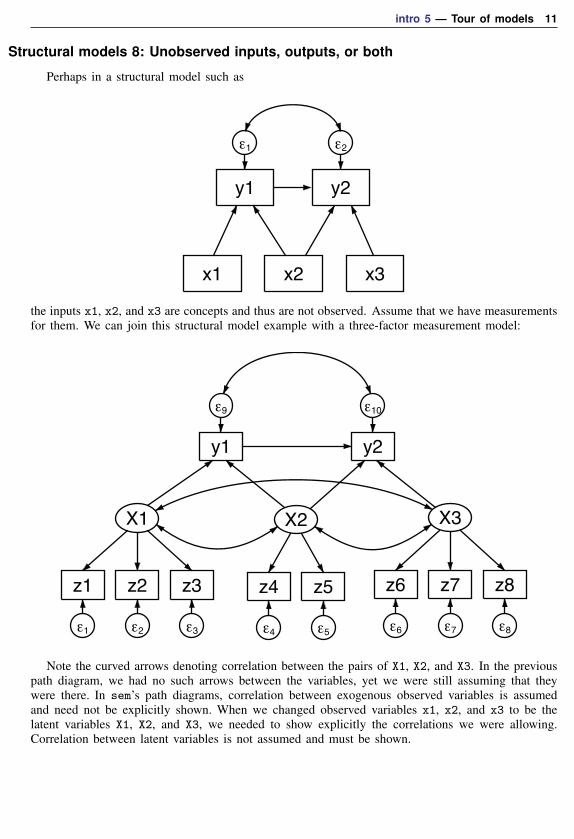
Structural models 8: Unobserved inputs, outputs, or both

Perhaps in a structural model such as

x1 x2 x3

y1

ε1

y2

ε2

the inputs x1, x2, and x3 are concepts and thus are not observed. Assume that we have measurementsfor them. We can join this structural model example with a three-factor measurement model:

X1

z1

ε1

z2

ε2

z3

ε3

X2

z4

ε4

z5

ε5

X3

z6

ε6

z7

ε7

z8

ε8

y1

ε9

y2

ε10

Note the curved arrows denoting correlation between the pairs of X1, X2, and X3. In the previouspath diagram, we had no such arrows between the variables, yet we were still assuming that theywere there. In sem’s path diagrams, correlation between exogenous observed variables is assumedand need not be explicitly shown. When we changed observed variables x1, x2, and x3 to be thelatent variables X1, X2, and X3, we needed to show explicitly the correlations we were allowing.Correlation between latent variables is not assumed and must be shown.

12 intro 5 — Tour of models

This model can be written in Stata command syntax as follows:

(y1<-X1 X2) (y2<-y1 X2 X3) ///(X1->z1 z2 z3) ///(X2->z4 z5) ///(X3->z6 z7 z8), ///

cov(e.y1*e.y2)

We did not include the cov(X1*X2 X1*X3 X2*X3) option, although we could have. In thecommand language, exogenous latent variables are assumed to be correlated with each other. If wedid not want X2 and X3 to be correlated, we would need to include the cov(X2*X3@0) option.

We changed x1, x2, and x3 to be X1, X2, and X3. In command syntax, variables beginning with acapital letter are assumed to be latent. Alternatively, we could have left the names in lowercase andspecified the identities of the latent variables:

(y1<-x1 x2) (y2<-y1 x2 x3) ///(x1->z1 z2 z3) ///(x2->z4 z5) ///(x3->z6 z7 z8), ///

cov(e.y1*e.y2) ///latent(x1 x2 x3)

Just as we have joined an observed structural model to a measurement model to handle unobservedinputs, we could join the above model to a measurement model to handle unobserved y1 and y2.

Models with unobserved inputs, outputs, or both can be fit by sem and gsem.

See the following examples:

1. [SEM] example 9. Structural model with measurement component.

2. [SEM] example 32g. Full structural equation model (generalized response).

4. [SEM] example 45g. Heckman selection model.

5. [SEM] example 46g. Endogenous treatment-effects model.

Structural models 9: MIMIC models

MIMIC stands for multiple indicators and multiple causes. An example of a MIMIC model is

L

ε1

i1 ε2

i2 ε3

i3 ε4c3

c2

c1

In this model, the observed causes c1, c2, and c3 determine latent variable L, and L in turn determinesthe observed indicators i1, i2, and i3.

intro 5 — Tour of models 13

This model can be written in Stata command syntax as

(i1 i2 i3<-L) (L<-c1 c2 c3)

MIMIC models can be fit by sem and gsem.

See the following examples:

1. [SEM] example 10. MIMIC model.

2. [SEM] example 36g. MIMIC model (generalized response).

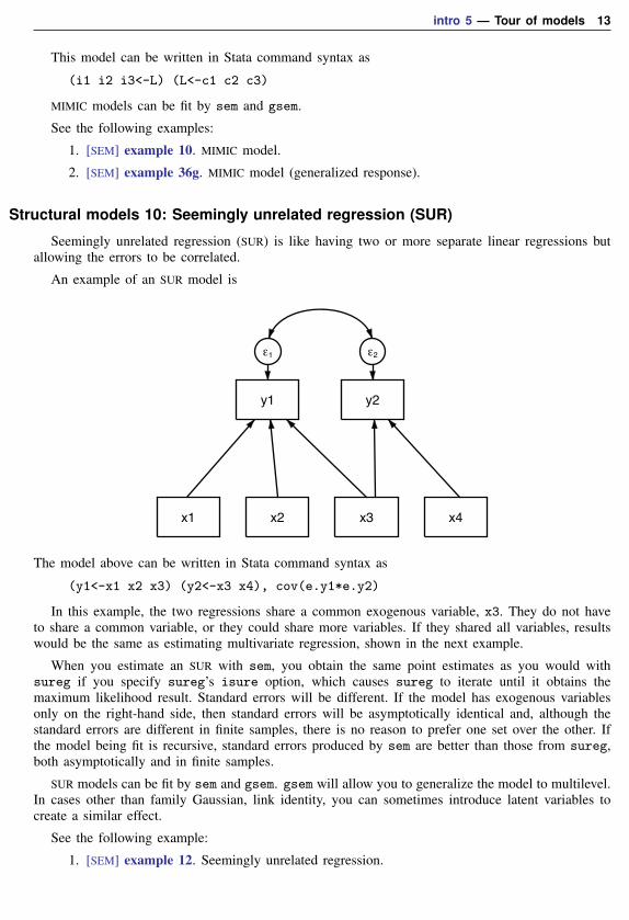
Structural models 10: Seemingly unrelated regression (SUR)

Seemingly unrelated regression (SUR) is like having two or more separate linear regressions butallowing the errors to be correlated.

An example of an SUR model is

x1 x2 x3 x4

y1

ε1

y2

ε2

The model above can be written in Stata command syntax as

(y1<-x1 x2 x3) (y2<-x3 x4), cov(e.y1*e.y2)

In this example, the two regressions share a common exogenous variable, x3. They do not haveto share a common variable, or they could share more variables. If they shared all variables, resultswould be the same as estimating multivariate regression, shown in the next example.

When you estimate an SUR with sem, you obtain the same point estimates as you would withsureg if you specify sureg’s isure option, which causes sureg to iterate until it obtains themaximum likelihood result. Standard errors will be different. If the model has exogenous variablesonly on the right-hand side, then standard errors will be asymptotically identical and, although thestandard errors are different in finite samples, there is no reason to prefer one set over the other. Ifthe model being fit is recursive, standard errors produced by sem are better than those from sureg,both asymptotically and in finite samples.

SUR models can be fit by sem and gsem. gsem will allow you to generalize the model to multilevel.In cases other than family Gaussian, link identity, you can sometimes introduce latent variables tocreate a similar effect.

See the following example:

1. [SEM] example 12. Seemingly unrelated regression.

14 intro 5 — Tour of models

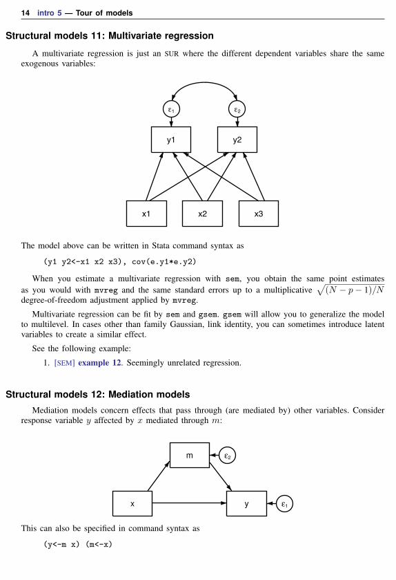
Structural models 11: Multivariate regression

A multivariate regression is just an SUR where the different dependent variables share the sameexogenous variables:

x1 x2 x3

y1

ε1

y2

ε2

The model above can be written in Stata command syntax as

(y1 y2<-x1 x2 x3), cov(e.y1*e.y2)

When you estimate a multivariate regression with sem, you obtain the same point estimatesas you would with mvreg and the same standard errors up to a multiplicative

√(N − p− 1)/N

degree-of-freedom adjustment applied by mvreg.

Multivariate regression can be fit by sem and gsem. gsem will allow you to generalize the modelto multilevel. In cases other than family Gaussian, link identity, you can sometimes introduce latentvariables to create a similar effect.

See the following example:

1. [SEM] example 12. Seemingly unrelated regression.

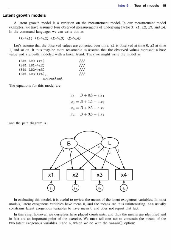
Structural models 12: Mediation models

Mediation models concern effects that pass through (are mediated by) other variables. Considerresponse variable y affected by x mediated through m:

x y ε1

m ε2

This can also be specified in command syntax as

(y<-m x) (m<-x)

intro 5 — Tour of models 15

In this simple model, x has a direct effect on y and an indirect (mediated through m) effect. Thedirect effect may be reasonable given the situation, or it may be included just so one can test whetherthe direct effect is present. If both the direct and indirect effects are significant, the effect of x issaid to be partially mediated through m.

There are one-level mediation models and various two-level models, and lots of other variations,too.

sem and gsem can both fit one-level linear models, but you will be better off using sem. gsemcan fit one-level generalized linear models and fit two-level (and higher) models, generalized linearor not.

See the following example:

1. [SEM] example 42g. One- and two-level mediation models (multilevel).

CorrelationsWe are all familiar with correlation matrices of observed variables, such as

x1 x2 x3

x1 1.0000x2 0.7700 1.0000x3 −0.0177 −0.2229 1.0000

or covariances matrices, such as

x1 x2 x3

x1 662.172x2 62.5157 9.95558x3 −0.769312 −1.19118 2.86775

These results can be obtained from sem. The path diagram for the model is

x1 x2 x3

We could just as well leave off the curved paths because sem assumes them among observed exogenousvariables:

x1 x2 x3

Either way, this model can be written in Stata command syntax as

(<- x1 x2 x3)

That is, we simply omit specifying the target of the path, the endogenous variable.

16 intro 5 — Tour of models

If we fit the model, we will obtain the covariance matrix by default. correlate with thecovariance option produces covariances that are divided by N − 1 rather than by N . To match thiscovariance exactly, you need to specify the nm1 option, which we can do in the command languageby typing

(<- x1 x2 x3), nm1

If we want correlations rather than covariances, we ask for them by specifying the standardizedoption:

(<- x1 x2 x3), nm1 standardized

An advantage of obtaining correlation matrices from sem rather than from correlate is that youcan perform statistical tests on the results, such as that the correlation of x1 and x3 is equal to thecorrelation of x2 and x3.

If you are willing to assume joint normality of the variables, you can obtain more efficient estimatesof the correlations in the presence of missing-at-random data by specifying the method(mlmv) option.

Correlations are fit using sem.

See the following example:

1. [SEM] example 16. Correlation.

Higher-order CFA models

Observed values sometimes measure traits or other aspects of latent variables, so we insert anew layer of latent variables to reflect those traits or aspects. We have measurements—say, x1, . . . ,x6—all reflecting underlying factor F, but x1 and x2 measure one trait of F, x3 and x4 measureanother trait, and x5 and x6 measure yet another trait. This model can be drawn as

intro 5 — Tour of models 17

x1

ε1

x2

ε2

x3

ε3

x4

ε4

x5

ε5

x6

ε6

A ε7 B ε8 C ε9

F

The model can be written in command syntax as

(A->x1 x2) (B->x3 x4) (C->x5 x6) (A B C<-F)

Higher-order CFA models can be fit using sem or gsem.

See the following example:

1. [SEM] example 15. Higher-order CFA.

Correlated uniqueness model

Observed values sometimes are correlated just because of how the data are collected. Imaginewe have factor T1 representing a trait with measurements x1 and x4. Perhaps T1 is aggression, andthen x1 is self reported and x4 is reported by the spouse. Imagine we also have factor T2 withmeasurements x2 and x5. Again, x2 is self reported and x5 is reported by the spouse. It would notbe unlikely that x1 and x2 are correlated and that x4 and x5 are correlated. That is exactly what thecorrelated uniqueness model assumes:

18 intro 5 — Tour of models

x1

ε1

x2

ε2

x3

ε3

x4

ε4

x5

ε5

x6

ε6

x7

ε7

x8

ε8

x9

ε9

T1 T2 T3

Data that exhibit this kind of pattern are known as multitrait–multimethod (MTMM) data. Researchershistorically looked at the correlations, but structural equation modeling allows us to fit a model thatincorporates the correlations.

The above model can be written in Stata command syntax as

(T1->x1 x4 x7) ///(T2->x2 x5 x8) ///(T3->x3 x6 x9), ///

cov(e.x1*e.x2 e.x1*e.x3 e.x2*e.x3) ///cov(e.x4*e.x5 e.x4*e.x6 e.x5*e.x6) ///cov(e.x7*e*x8 e.x7*e.x9 e.x8*e.x9)

An alternative way to type the above is to use the covstructure() option, which we can abbreviateas covstruct():

(T1->x1 x4 x7) ///(T2->x2 x5 x8) ///(T3->x3 x6 x9), ///

covstruct(e.x1 e.x2 e.x3, unstructured) ///covstruct(e.x4 e.x5 e.x6, unstructured) ///covstruct(e.x7 e.x8 e.x9, unstructured)

Unstructured means that the listed variables have covariances. Specifying blocks of errors as unstruc-tured would save typing if there were more variables in each block.

The correlated uniqueness model can be fit by sem or gsem, although we recommend use of sem inthis case. Gaussian responses with the identity link are allowed to have correlated uniqueness (error)but only in the absence of censoring. gsem still provides the theoretical ability to fit these models inmultilevel contexts, but convergence may be difficult to achieve.

See the following example:

1. [SEM] example 17. Correlated uniqueness model.

intro 5 — Tour of models 19

Latent growth models

A latent growth model is a variation on the measurement model. In our measurement modelexamples, we have assumed four observed measurements of underlying factor X: x1, x2, x3, and x4.In the command language, we can write this as

(X->x1) (X->x2) (X->x3) (X->x4)

Let’s assume that the observed values are collected over time. x1 is observed at time 0, x2 at time1, and so on. It thus may be more reasonable to assume that the observed values represent a basevalue and a growth modeled with a linear trend. Thus we might write the model as

(B@1 L@0->x1) ///(B@1 L@1->x2) ///(B@1 L@2->x3) ///(B@1 L@3->x4), ///

noconstant

The equations for this model are

x1 = B + 0L+ e.x1

x2 = B + 1L+ e.x2

x3 = B + 2L+ e.x3

x4 = B + 3L+ e.x4

and the path diagram is

x1

ε1

x2

ε2

x3

ε3

x4

ε4

B L

1

0

11

1

2

1

3

In evaluating this model, it is useful to review the means of the latent exogenous variables. In mostmodels, latent exogenous variables have mean 0, and the means are thus uninteresting. sem usuallyconstrains latent exogenous variables to have mean 0 and does not report that fact.

In this case, however, we ourselves have placed constraints, and thus the means are identified andin fact are an important point of the exercise. We must tell sem not to constrain the means of thetwo latent exogenous variables B and L, which we do with the means() option:

20 intro 5 — Tour of models

(B@1 L@0->x1) ///(B@1 L@1->x2) ///(B@1 L@2->x3) ///(B@1 L@3->x4), ///

noconstant means(B L)

We must similarly specify the means() option when using the Builder.

Latent growth models can be fit with sem or gsem.

See the following example:

1. [SEM] example 18. Latent growth model.

Models with reliability

A typical solution for dealing with variables measured with error is to find multiple measurementsand use those measurements to develop a latent variable. See, for example, Single-factor measurementmodels and Multiple-factor measurement models above.

When the reliability of the variables is known—reliability is measured as the fraction of variancesthat is not due to measurement error—another approach is available. This approach can be usedin place of or in addition to the use of multiple measurements. See [SEM] sem and gsem optionreliability( ).

Models with reliability can be fit with sem or gsem, although option reliability() is availableonly when responses are Gaussian with the identity link and only in the absence of censoring.

See the following example:

1. [SEM] example 24. Reliability.

Multilevel mixed-effects modelsMultilevel modeling concerns the inclusion of common, random effects across groups of the data,

which are known as levels. You have observations on students. Students attend schools. Or you haveobservations on patients. Patients are served by hospitals. In either case, there may be an unmeasuredeffect of the institution. Some schools are better than others while some schools are worse. Thesame applies to hospitals. These unmeasured effects can be parameterized as a latent variable that isconstant within institution and varies across institution.

What we have just described is a two-level nested model. The first level, the lowest, is theobservational level. The second level is school or hospital.

In a three-level nested model, students are served by schools which are served by counties, or patientsare served by hospitals which are served by states. Whatever the example, there can be unmeasuredeffects of each of those higher levels contributing to the effect observed at the observational level.

An alternative to nested models is crossed models. People with jobs work in an industry and ina state. The same industries are found across states and the same states are found across industries,yet both may have an effect on some aspect of the lives of their workers.

intro 5 — Tour of models 21

Multilevel models are fit by gsem.

See the following examples:

1. [SEM] example 30g. Two-level measurement model (multilevel, generalized response).

2. [SEM] example 38g. Random-intercept and random-slope models (multilevel).

3. [SEM] example 39g. Three-level model (multilevel, generalized response).

4. [SEM] example 40g. Crossed models (multilevel).

5. [SEM] example 41g. Two-level multinomial logistic regression (multilevel).

6. [SEM] example 42g. One- and two-level mediation models (multilevel).

ReferencesAcock, A. C. 2013. Discovering Structural Equation Modeling Using Stata. Rev. ed. College Station, TX: Stata Press.

Bauldry, S. 2014. miivfind: A command for identifying model-implied instrumental variables for structural equationmodels in Stata. Stata Journal 14: 60–75.

Bollen, K. A. 1989. Structural Equations with Latent Variables. New York: Wiley.

Also see[SEM] intro 4 — Substantive concepts

[SEM] intro 6 — Comparing groups (sem only)

[SEM] example 1 — Single-factor measurement model