Embed Size (px)
Citation preview

1
Title: Quality of presence data determines species distribution model performance: a novel index 1
to evaluate data quality 2
3
Running title: A novel index to evaluate data quality 4
5
Authors: Songlin Fei* and Feng Yu 6
Department of Forestry and Natural Resources, Purdue University 7
8
*Correspondence: Songlin Fei, PFEN221E, Purdue University, 715 W. State St., West Lafayette, 9 IN, USA, 47907. Email: [email protected] 10
11
Date of manuscript draft: August 18, 2015 12
13
Manuscript Word Count: 5138 14
15
Number of Figures: 5 16
17

2
ABSTRACT 18
Context Species distribution models (SDMs) are widely used to estimate species’ potential 19
distribution at landscape to regional scales. However, the quality of occurrence data is often 20
compromised by sampling bias. The negligence of data quality assessment could raise serious 21
concerns on model accuracy. 22
Objectives. We propose a model-independent composite measure - representativeness and 23
completeness (RAC) index - to evaluate the quality of species occurrence data. We demonstrate 24
(1) the impact of spatial data quality as measured by RAC on model performance and (2) the 25
feasibility of applying RAC in actual modeling process. 26
Methods. By using a set of computational experiments on a virtual species, we calculated 27
RAC values for a set of occurrence data (35 runs x 50 datasets x 5 series) representing different 28
degrees of sampling biases. We evaluated model performance (reliability and accuracy) using 29
three different model algorithms; and we associated model performance with RAC values. Two 30
case studies were also conducted to demonstrate the association between RAC and model 31
performance. 32
Results. Model reliability stabilizes when RAC reaches a threshold of 0.4. Model 33
accuracy also stabilizes when RAC reaches 0.4 or 0.5 for models with or without complete 34
predictors, respectively. Model performance is more sensitive (i.e., has larger variability) to data 35
completeness than representativeness. Our case studies further demonstrated that RAC value is 36
closely related to model performance. 37
Conclusions. Performance of SDMs is closely related to the quality of species occurrence data, 38
which can be measured by our model-independent composite index - RAC. We recommend a 39
minimum RAC value of 0.4 for reliable and accurate SDM predictions. To improve prediction 40

3
accuracy, sampling with multiple centers in a systematic fashion across the environmental space 41
is desired. 42
43
Keywords Species distribution modeling, data quality, representativeness, completeness 44
45

4
INTRODUCTION 46
Species distribution models (SDMs) estimate the relationship between species occurrence or 47
abundance with the corresponding environmental conditions using a set of statistical methods 48
(Elith and Leathwick 2009). Due to the wide availability of species occurrence data and efficient 49
modeling tools, SDMs have received increasing attention from forecasting risk of biological 50
invasions and impacts of climate change to spatial conservation planning and historical 51
biogeography, with thousands of papers being published annually (Franklin 2013). The products 52
of SDMs, usually the predicted distribution maps or habitat suitability maps at landscape to 53
regional-scales, often serve as the foundation and possibly the only reliable information for 54
conservation planning, risk assessment, or resource management implementations (Franklin 55
2009). 56
57
However, the quality of species distribution data is often compromised by sampling bias in terms 58
of spatial distribution, especially for presence-only data. For example, sampling intensity may 59
not be consistent across regions. Some regions are under-sampled due to poor site accessibility 60
or incomprehensive survey plan, while other regions are over-sampled (Peterson and Holt 2003; 61
Phillips et al. 2006). In addition, sometime only part of the presence data was used in the 62
modeling process. Therefore, the accuracy and reliability of SDMs are likely compromised by 63
incomplete or biased survey data. 64
65
Paradoxically, the lack of comprehensive observations is probably the most important reason for 66
using SDMs to extend the data availability for conservation planning and resource management 67
purposes, predicting species distributions in the remote areas that field surveys are not able to 68

5
cover. To improve the performance of SDMs based on ‘imperfect’ species distribution data, a 69
set of methodological approaches have been advanced in the recent years, such as sampling bias 70
correction (Kramer-Schadt et al. 2013), data quality discrimination (Hortal et al. 2001), 71
appropriate predictor selection and model parameterization (Elith and Leathwick 2009; Merow et 72
al. 2013), and consensus forecasting (Araújo and New 2007). However, inherent limitations of 73
the sampling data cannot be fully corrected only through these approaches (Merow et al. 2013; 74
Phillips and Elith 2013). 75
76
This raises an important question addressed in this paper: can we estimate model performance, 77
both in reliability and accuracy, based on the quality of species occurrence data prior to the 78
application of SDMs? Among many components of SDMs, species occurrence data are the 79
foundation for the prediction of species occurrence probability or habitat suitability. Therefore, 80
the quality of the occurrence data can be a decisive contributor for the performance of SDMs. 81
Currently, limited systematic frameworks have been suggested to evaluate the quality of species 82
distribution data used for SDMs (but see Hortal and Lobo 2005; Lobo and Martín‐Piera 2002; 83
Luoto et al. 2005; Reese et al. 2005), and no quantitative tool is available to evaluate the quality 84
of species distribution data. 85
86
The key questions in evaluating the quality of occurrence data are: what are the most important 87
factors that influence the quality of species distribution data, and how can the quality of species 88
distribution data be quantitatively assessed? Fortunately, all existing SDMs share one important 89
characteristic -- they are essentially all statistical models (Austin 2007; Elith et al. 2006). These 90
statistical models require two underlying assumptions to comply with the basis of ecological 91

6
niche theory: (1) the sampling occurrence should be representative of the extent of the ecological 92
niche in the environmental space (whether it is in a fundamental or realized niche depends on the 93
model method) and (2) the sampling occurrence should be at equilibrium, covering the entire 94
extent of the ecological niche in the environmental space (Araújo and Pearson 2005; Guisan and 95
Thuiller 2005). Representativeness is defined as the sampling data being randomly distributed 96
throughout the ecological niche; while equilibrium is defined as the occurrence data 97
comprehensively covering the entire niche and being absent in the locations outside of the niche, 98
which we refer to as completeness (Araújo and Pearson 2005; Guisan and Thuiller 2005; 99
Václavík and Meentemeyer 2012). Although the two assumptions are rarely satisfied in actual 100
survey data (Acevedo et al. 2012), they can be used to quantify the quality of species distribution 101
data, especially presence-only data. More specifically, we can calculate the degree of 102
representativeness and completeness of the data in the environmental space of known niche or 103
observed occurrence range. 104
105
In this study, we proposed a novel quantitative measure, representativeness and completeness 106
(RAC) index, to assess SDMs’ predictive reliability and accuracy based on the two assumptions 107
mentioned above by focusing only on the characteristics of species occurrence data. The 108
application of RAC will allow modelers to determine the quality of occurrence data and the 109
confidence of modeling results independent of SDMs. We studied the relationship between the 110
sampling pattern of occurrence data in the environmental space (constructed by bioclimatic 111
variables) and model performance. Our hypothesis is that the quality of occurrence data, as 112
measured by our RAC index, is positively related to model performance. By focusing on the 113
occurrence data, modelers can discern a very basic but essential assessment of the ‘usefulness’ of 114

7
their data and the expected accuracy and reliability. We expect this study will greatly benefit the 115
research and practices of the macrosystem ecology, biogeography, and conservation community 116
by avoiding seriously biased or incorrect model outputs that are based on species distribution 117
data of unsatisfactory quality. 118
119
METHODS 120
We examined the influence of occurrence data quality on model performance by using a virtual 121
species living in a scaled environmental space with the following major steps. First, we created a 122
gradient of occurrence patterns representing different degrees of sampling biases, and measured 123
the corresponding data quality with RAC. Second, we evaluated model performance (reliability 124
and accuracy) for three different model algorithms using the ‘binned’ evaluation method for each 125
datasets. Third, the relationship between data quality and model performance was analyzed and 126
critical thresholds of RAC were identified where the model performance was significantly 127
improved and stabilized. 128
129
Virtual species in a scaled environmental space 130
We created a virtual species living in a scaled environmental space. Two environmental 131
variables (predictors): temperature (T) and precipitation (P), both scaled with a range of 0 to 1, 132
were used to create the environmental space (akin to Phillips and Elith 2010). The extent of this 133
environmental space includes all existing environmental conditions that occurred in all known or 134
observed areas, which is equivalent to the ‘biotope’ according to the classic niche concept of 135
Hutchinson (Franklin 2009). We assumed that the true probability of presence of this virtual 136
species is defined as pT = (T+P)/2 in this environmental space. The utilization of this scaled 137
8
environmental space allows our findings to be applicable to both generalist and specialist species 138
since the niche studied here is in a relative scale (0 to 1) regardless of its actual niche width. 139
140
Point pattern gradients 141
We designed five data series to represent possible spatial distribution patterns of sample 142
locations. To clarify, the simulated point patterns in the following procedure are not the 143
representations of the underlying species distribution, which could have different patterns (e.g., 144
clustered, random, etc.) that are often species or taxonomic groups specific; rather, the simulated 145
patterns are the representations of possible sampling results due to different degree of sampling 146
biases. 147
148
Each of the five data series has 50 unique point patterns that evolve gradually from highly 149
clustered to completely random following the method by Ong et al. (2012) (Figure 1). In order 150
to obtain a continuous and gradual transition, each point pattern was created by combining point 151
samples from a random distribution in one or several grid squares (Z1) and the complimentary 152
subareas (Z2, which is the total area minus Z1) of the environmental space (Ong et al. 2012). 153
Because sample size could be an important factor influencing model performance where small 154
sample size (n<30) cannot produce consistent predictions (Wisz et al. 2008), we used a total of 155
1,000 points to generate each point pattern to ensure sample size will not impact our analysis. 156
Z1 contains 990 point locations and Z2 contains 10 point locations (see Appendix 1 for detailed 157
procedure for point pattern generation). We used the ‘Create Random Points’ tool in ArcMap 158
(ESRI, Redlands, CA, USA) to generate the random point patterns in Z1 and Z2 with a Poisson 159
distribution. 160

9
Although each dataset was generated through combining random points from Z1 and Z2, our 161
preliminary analysis indicated that it did not completely eliminate the possibility of regional 162
pattern bias in the environmental space (e.g., highly clustered in one subarea of Z1). Therefore, 163
to reduce the possible spatial bias due to random chances, we ran 7 iterations to generate 164
different sets of random points (i.e., each iteration generates different point patterns representing 165
locations of presence/pseudo-absence of the virtual species for each of the 50 datasets in each 166
series). ‘Presence’ or ‘absence’ of each point was determined via Bernoulli trials (0 and 1) based 167
on the occurrence probability (PT) at a given location. Note that the term ‘absence’ was not 168
intended to represent the locations where the environmental conditions were not suitable for this 169
virtual species; rather, it was used to simulate modeling procedure that based only on presence 170
data (Franklin 2009; Phillips et al. 2009). 171
172
To simulate the presence/absence at a given point due to random chances (i.e., presence of a 173
given species may not be observed at a given location during one sampling effort due to random 174
effects), we ran 5 replications (5 sets of Bernoulli trials) to assign presence/absence values for 175
each of the 7 iterations. Therefore, each of the 50 datasets in each series has a total of 35 runs of 176
occurrence patterns, allowing sufficient statistical power given our computational capacity (5 177
series x 50 datasets/series x 7 iterations/dataset x 5 runs/iteration = 8,750 runs). Data analyses 178
were conducted on each of the 8,750 runs. 179
180
Measurement of species distribution data quality 181
We created a composite measure - RAC (representativeness and completeness) index - to 182
quantify the quality of species distribution data. RAC includes the calculation of nearest 183

10
neighbor statistics (a measure of representativeness) and completeness ratio (a measure of 184
completeness). The completeness ratio is the degree of coverage of the observed species 185
occurrence in the corresponding environmental space of its known or observed niche. For a two-186
dimensional environmental space, the completeness ratio (Ω) can be calculated by multiplication 187
of the completeness of each dimension as follows: 188
189
where is the observed occurrence range of the environmental variable i, and Ni is the 190
corresponding known or observed niche described by the environmental variable i. The range of 191
varies from 0 to 1, which reflects the degree of completeness (Kadmon et al. 2003). 192
193
We used nearest neighbor statistic (R) to measure representativeness based only on occurrence 194
localities (presence points). The core concept of nearest neighbor analysis is to calculate the 195
mean Euclidean distances between each paired nearest neighbors, and then compare the result 196
with the expected or theoretical situation. According to Clark and Evans (1954), the mean of 197
observed distance Do can be calculated as: 198
∑
199
where ri is the distance for the ith point to its paired nearest neighbor and N is the total number of 200
points in the environmental space. The expected mean nearest neighbor distance De in a uniform 201
random distribution can be calculated as: 202
12
203
11
where A is the total area of the environmental space in the known or observed niche and n is the 204
number of points. The reason we used uniform random distribution to calculate De is that the 205
critical assumption required for presence-only data based SDMs is the random sampling of space 206
for accumulating presence only observations (Royle et al. 2012). Nearest neighbor statistic (R) is 207
the ratio of observed ( ) to expected ( ) mean nearest neighbor distance (R = Do/De). R 208
approaches to 0 if the point pattern is completely clustered, and R approaches to 1 if the point 209
pattern is uniform random (Clark and Evans 1954, see Appendix 2 for examples). Our 210
composite measure (RAC) of the spatial pattern of the species distributions localities was defined 211
as the product of completeness ( ) and the nearest neighbor statistic ( ), 212
213
RAC varies from 0 (total deviation from completeness and representativeness) to 1 (perfect 214
completeness and representativeness). 215
216
Simulation of SDMs 217
We designed three model algorithms to simulate different possible scenarios of actual modeling 218
methods in terms of the selection of environmental variables akin to Phillips and Elith (2010). 219
Model 1, p1 = 0.25 + 0.5 T, estimates the probability of species occurrence only based on 220
temperature. In practice, this could result from some of the essential predictors controlling the 221
species distribution not being correctly identified or some predictors being mistakenly excluded 222
due to a certain SDM method (Phillips and Elith 2010). Model 2, p2 = 0.25 (T + P) + 223
0.125 (T + P)2, estimates the probability of presence from both of the variables (T and P) as a 224
comprehensive suite of the possible combinations of the environmental variables including 225
interaction terms. Model 3, p3 = (T+P)/2, is the ‘true’ probability of presence of the species. 226

12
Model evaluation 227
Model performance is generally described as predictive accuracy, which has two components: 228
discrimination and calibration (Vaughan and Ormerod 2005). Discrimination is the ability of the 229
model to correctly distinguish occupied from unoccupied sites, whereas calibration measures the 230
agreement between predicted probabilities of occurrence and observed proportions of sites 231
occupied (Pearce and Ferrier 2000). In this study, we focused only on calibration - the numerical 232
accuracy of prediction (Phillips and Elith 2010; Vaughan and Ormerod 2005). Discrimination 233
was not calculated because there is no true absence in our environmental space. 234
235
Calibration can be examined graphically via a ‘binned’ method (Pearce and Ferrier 2000; 236
Vaughan and Ormerod 2005) by plotting the median values of predicted probabilities in each of 237
the predefined predicted probability intervals against the fraction of the actual observed localities 238
(marked as ‘presence’) vs. the total localities within each of these probability intervals (see 239
example in Appendix 3). The overall calibration across all the predicted probability intervals, 240
which indicates the general model performance, can be obtained from the slops of a linear 241
regression line of these plots. In general, slope = 1 indicates good model calibration, slope > 1 242
indicates underestimation, and slope <1 indicates overestimation (Vaughan and Ormerod 2005). 243
In this study, we divided the predicted probability into 10 intervals and plotted the median in 244
each interval against the fraction of the actual observed localities. 245
246
Association between model performance and data quality 247
To analyze the association between model performance and RAC, we plotted the mean and 248
standard error of the slopes from the linear regression of the binned method against the mean 249
13
RAC value of the 35 runs in each dataset for all three models (Figure 2). Mean of the slope was 250
used to measure the accuracy (average slope approaching 1 indicates high accuracy); while 251
standard error of the slope was used to measure model reliability (standard error is minimized for 252
all 35 runs when models are reliable). In addition, we used multivariate adaptive regression 253
splines (MARS) to further illustrate the relationships between RAC values and model reliability 254
and accuracy, and to detect critical RAC thresholds where model performance are significantly 255
improved. 256
257
RESULTS 258
In general, we found that both model reliability and accuracy increase with data quality as 259
measured by RAC (Figure 2). As point pattern evolves from highly clustered to near uniform 260
random, model performance improves. Note that the trend does not proceed gradually along the 261
point pattern gradient. Instead, model performance, in terms of both model reliability (Figure 262
2a) and accuracy (Figure 2b), ‘jumps’ or ‘turns’ significantly at certain critical RAC values. 263
These critical points serve as important indicators of model performance for different model 264
algorithms and point patterns. 265
266
Model reliability dramatically improves as RAC value approaches to 0.4, and stabilizes after this 267
threshold regardless of model algorithms or spatial point patterns (Figures 2a and 3a). Model 268
accuracy also follows the same trend. Model accuracy improves as RAC value approaches to the 269
thresholds [0.40 for models with completed environmental variables (Model 2 and Model 3) and 270
0.50 for models missing key environmental variables (Model 1)], and stabilizes after that 271

14
(Figures 2b and 3b). All models, except Model 1 in Series E, have an accuracy of greater than 272
0.7 after RAC value reaching the above thresholds (Figure 4). 273
274
Of the two components that defines RAC index, both representativeness and completeness 275
values are positively related to model accuracy; while model performance is more sensitive (i.e., 276
has larger variability) to data completeness than representativeness (Figure 5). Model accuracy 277
becomes stable when representativeness value reaches 0.40 for models with completed 278
environmental variables (Model 2 and Model 3) and 0.85 for models missing key environmental 279
variables (Model 1) (Figure 5a). Whereas model accuracy becomes stable only after 280
completeness value reaches 0.95 for all models (Figure 5b). 281
282
Spatial pattern of presence-only data has a strong influence on model performance. Models in 283
series A have higher accuracy and reliability than any other series (Figures 2 and 4). In general, 284
both model accuracy and reliability are high even when RAC value is below the threshold. This 285
is because data in series A have multiple clusters (9 total) evenly-distributed across the 286
environmental space of the virtual species; while data in other series have a single cluster. This 287
again confirms our hypothesis that model performance is very sensitive to the spatial distribution 288
of species occurrence data, and even to how the points are clustered spatially. 289
290
Models with complete environmental variables (Model 2 and 3), regardless of whether 291
interactions were included in the model, often achieve model stability easier (with lower RAC 292
values) than models that lack one or more essential environmental variables (Model 1) (Figure 293
2). Model 1 is designed to simulate the possible practical scenario that some important variables 294
15
are not selected in the modeling process or the model mistakenly excluded some environmental 295
variables. This indicates the importance of predictor selection since models with incomplete 296
environmental predictors require a higher degree of completeness and representativeness from 297
the distribution data to achieve better model performance, which in turn increases the cost and 298
workload of conducting species survey. 299
300
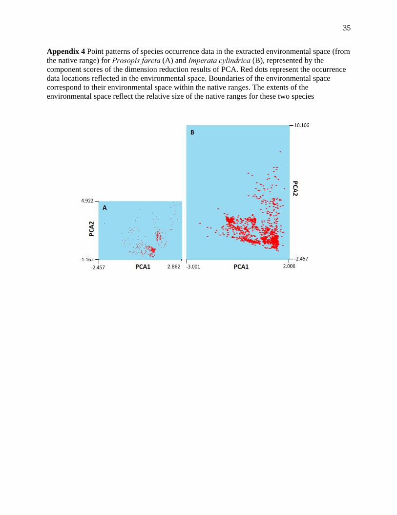
CASE STUDIES 301
To demonstrate the use of RAC to measure the quality of species distribution data and its 302
implications of model performance, we modeled the habitat suitability of two invasive species, 303
Prosopis farcta (PRFA) and Imperata cylindrica (IMCY). Presence data of the two species were 304
obtained from the Global Biodiversity Information Facility (GBIF, www.gbif.org/), a widely 305
used database for SDMs. Native ranges for these two species were used to define their 306
ecological niches. IMCY was selected to represent the case of poor quality of presence data 307
since the presence data were clustered in a portion of its native range in the environmental space 308
even though it has a large sample size (n= 4,913); while PRFA was selected (n=281) to represent 309
better data quality in terms of spatial coverage. 310
311
Unlike the virtual species modeled above in the idealized landscape, where environmental space 312
overlaps with geographical space, we need to convert the environmental variables within the 313
geographical range to environmental space to calculate RAC for actual species. First, we 314
obtained six environmental variables (annual mean temperature, isothermality, mean temperature 315
of coldest quarter, annual mean precipitation, coefficient of variation of monthly precipitation, 316
and precipitation of driest quarter) from WorldClim (http://www.worldclim.org, Hijmans et al. 317

16
2005) based on knowledge from variable selections of other studies (Austin 2007; Austin and 318
Smith 1989; Elith and Leathwick 2009). Second, we used principal component analysis (PCA) 319
on these six variables to reduce the environmental dimensions to two orthogonal components. 320
We measured the correlation among the six variables to ensure that the data were suitable for 321
PCA. The results indicated that in the correlation matrix, each variable had at least one 322
correlation coefficient > 0.3 and the overall Kaiser-Meyer-Olkin (KMO) value was >0.5, 323
satisfying the minimum requirement for conducting a PCA (Kaiser 1974). The two major 324
components, PCA1 and PCA2, explained 59.85% and 22.84% of the variability for PRFA and 325
51.84% and 24.61% for IMCY, respectively. Third, species occurrence data were then re-plotted 326
onto the new two-dimensional environmental space (Appendix 4), and their RAC values were 327
calculated using the procedure described in the methods section. 328
329
To compare RAC value with other model performance indicators, we used MaxEnt (Version 330
3.3.3k, Phillips et al. 2006) to model the spatial distribution of PFRA and IMCY based on the 331
same presence data and six environmental variables mentioned above. ‘Target Group’ 332
background method was applied to reduce the sampling bias, as suggested by Phillips et al. 333
(2009). We used 38 species from our invasive species study (unpublished data) to compose the 334
locations of the target-group background. Area Under Curve (AUC) and True Skill Statistics 335
(TSS) were used to evaluate the model performance (Allouche et al. 2006; Pearce and Ferrier 336
2000). AUC is a single-value, threshold-independent indicator of the general model performance 337
that is not influenced by species prevalence (Manel et al. 2001; Pearson et al. 2013). However, 338
AUC is not sensitive to the shift of model accuracy and a poorly fitted model may also receive 339
high AUC value (Lobo et al. 2008). On the other hand, although TSS is a threshold-dependent 340
17
evaluation method, it provides the ability to distinguish between a well fitted model and poorly 341
fitted model, which is also not influenced by the species prevalence (Allouche et al. 2006). We 342
used Maximum Sensitivity plus Specificity (MSS, Jiménez-Valverde and Lobo 2007) to 343
determine the ‘presence-absence’ threshold to calculate TSS. AUC and TSS are complementary 344
and reflect different perspectives of model performance. 345
346
Results from the case studies further illustrated that RAC value is positively associated with 347
model performance. RAC value for PRFA is 0.449 (high degree of completeness, Ω = 0.830 and 348
evenness, R = 0.541). Correspondingly, AUC and TSS for PRFA were 0.991 and 0.902, 349
respectively, indicating good model performance. RAC value for IMCY is 0.215 (lower degree 350
of completeness, Ω = 0.600 and evenness, R = 0.358). Correspondingly, AUC and TSS for 351
IMCY were 0.890 and 0.656, respectively, indicating poor model performance. Larger 352
differences were observed in TSS values than AUC. This is likely due to effect of prevalence of 353
species occurrence (sample size of IMCY was much larger than PRFA), which may result in the 354
falsely higher AUC (Allouche et al. 2006). 355
356
DISCUSSION 357
358
In this study, we demonstrated that the quality of species distribution data is closely associated 359
with the performance of SDMs. Our results clearly revealed that RAC values are positively 360
correlated with model performance in both reliability and accuracy. In general, model 361
performance stabilizes when RAC reaches 0.40 for models include all necessary environmental 362
variables, regardless of model algorithm used. 363
18
The correlation between RAC and predictive accuracy clearly confirmed the conclusion from 364
other studies that sampling bias has a profound impact on predictive accuracy (Kadmon et al. 365
2003). However, such sampling bias has been difficult to describe in the modeling work without 366
survey information, especially for the presence-only data. In this study, we quantitatively linked 367
sampling bias to the spatial point patterns of occurrence data in the environmental space. 368
Modelers can compare to the proposed thresholds and estimate what the predictive results will be 369
likely achieved when applying these data in their SDMs. 370
371
Research implications 372
Between the two components that determines RAC value, completeness is more sensitive to 373
model performance than representativeness. This partially explains the results that models in 374
series A have higher accuracy and reliability than any other series because data in series A have 375
multiple clusters (9 total) evenly-distributed across the environmental space, resulting a higher 376
completeness and representativeness values compared to data in other series that have a single 377
cluster. Our findings agree with a sampling bias correction study by Fourcade et al. (2014), who 378
found that among five sampling bias correction methods, simple systematic re-sampling (i.e., 379
subsample of records that are regularly distributed) of available data consistently outperformed 380
all other methods across various test conditions. 381
382
Our study clearly demonstrated the need of high quality primary data in order to achieve 383
subsequent accurate modeling results. As advocated by many prior studies (e.g., Hijmans 2012; 384
Lobo and Martín‐Piera 2002; Reese et al. 2005), we need well-designed surveys to obtain high 385
quality data for better model performance. We suggest the collection or utilization of data with 386

19
high spatial completeness and representativeness for accurate modeling performance if possible. 387
More specifically, data with multiple centers in a systematic fashion across the environmental 388
space can facilitate the faster achievement of the recommended RAC threshold than mono-389
centered data. 390
391
Research applications 392
We used a virtual species to demonstrate the necessity of high data quality for accurate and 393
reliable model performance. Although there are some challenges as often encountered in other 394
species modeling efforts, results from our computational experiments can be easily applied in 395
real situations with the following general steps: (1) convert data from geographic space to 396
environmental space; (2) measure RAC value of sample points in the environmental space, and 397
(3) compare the calculated RAC value with the recommended minimum RAC value. 398
399
Converting data from geographic space to environmental space can be conducted in two steps. 400
First, environmental variables that are closely related to the distribution of the target species 401
should be selected (e.g., Fei et al. 2012). Second, ordination methods such as principal 402
component analysis (PCA) or environmental niche factor analysis (ENFA, Hirzel et al. 2002) 403
need be used to reduce the environmental dimensions to two orthogonal components. The 404
resulting two orthogonal components can be used to represent the environmental space for the 405
target species. One of the main advantages of calculating RAC values in environmental space is 406
that moving from geographic to environmental space may reduce erroneous, or misleading, 407
“representativeness” values. For example, a species may be clustered in geographic space 408
because it requires specific environmental conditions that are also clustered on the landscape. 409

20
Conversion to environmental space should alleviate some of this spatial clustering. The 410
limitation of this approach is that sometimes the resulted primary and secondary components 411
cannot adequately represent the variability of the environmental space. 412
413
To measure RAC value in the converted environmental space, we first need to re-plot the 414
occurrence data onto the new two-dimensional environmental space and calculate RAC value 415
using the procedure described in the method section. However, it is not straight-forward to 416
define the boundaries of the environmental space or niche width (realized vs. fundamental 417
niches), a common challenge in species distribution models (Elith and Leathwick 2009; Sax et al. 418
2013). For our virtual species, we assumed that the fundamental niche, realized niche and 419
‘biotope’ are approximately equivalent. This may only apply to broad spatial scales and species 420
have reached distribution equilibrium. In practice, we recommend the use of range maps (an 421
approximation of realized niche) to define the boundaries of the environmental space, as range 422
maps are often available for many species in North America, Europe, and Asia. Digital range 423
maps (or to be digitized from paper versions) can be used to overlay on all environmental 424
variable layers to define environmental spaces. After the calculation of the RAC value for the 425
target species, we can compare it with the threshold value (RAC > 0.4) to determine if the data 426
quality is acceptable. 427
428
Cautions need be made when applying the proposed RAC index to assess data quality due to its 429
inherited limitations. Models used to predict species distribution often involve various 430
environmental variables such as climate, soil, terrain, geology, land use, and etc. These variables 431
often have their limitations on thematic, spatial, and temporal scales, and dimension reduction 432

21
using two principal components may not capture the variations of ecological niches. Both of 433
which can limit the feasibility of the application of the proposed 0.4 RAC threshold. On the 434
other hand, variables used in SDMs are often highly correlated (e.g., Fei et al. 2007; Liang and 435
Fei 2014) and climate factors are the first order variables that influence species ranges limits and 436
are often readily available (Ricklefs and Jenkins 2011; Shen et al. 2012). Therefore, we 437
recommend the application of the proposed RAC index primarily on bioclimatic variables as 438
demonstrated in our case studies. Additional research is needed to study the impact of the 439
inclusion of other non-climatic variables and the interplays among environmental variables on 440
RAC values and the subsequent model performance. 441
442
In conclusion, we demonstrated that the performance of SDMs, in terms of reliability and 443
accuracy, is closely related to the quality of species occurrence data. We provided a novel way 444
to evaluate data quality through a composite measure - RAC, which measures the degree of 445
proximity to ideal representativeness and completeness. Modelers can estimate the quality of 446
model results by calculating the RAC values of their occurrence data and comparing them with 447
the recommended critical thresholds (RAC > 0.4) prior to their modeling effort. Unlike other 448
commonly used model evaluation methods, RAC is model-independent. Modelers can use this 449
method to preselect and eliminate unsuitable species distribution data before running any model. 450
A user-friendly tool is needed to easily calculate the RAC value for various species and model 451
efforts for the benefit of the ecology, biogeography, and conservation communities. 452
453
ACKNOWLEDGMENT 454

22
We thank Drs. Janet Franklin, Jeffrey Dukes, Jane Frankenberger for helpful comments on an 455
earlier versions of the manuscript. We acknowledge funding support from the National Science 456
Foundation (Macrosystems Biology 1241932). 457
458
REFERENCES 459
Acevedo P, Jiménez-Valverde A, Lobo JM, Real R (2012) Delimiting the geographical 460
background in species distribution modelling. J. Biogeogr. 39(8):1383-1390 461
Allouche O, Tsoar A, Kadmon R (2006) Assessing the accuracy of species distribution models: 462
prevalence, kappa and the true skill statistic (TSS). J. Appl. Ecol. 43(6):1223-1232 463
Araújo MB, New M (2007) Ensemble forecasting of species distributions. Trends Ecol. Evol. 464
22(1):42-47 465
Araújo MB, Pearson RG (2005) Equilibrium of species’ distributions with climate. Ecography 466
28(5):693-695 467
Austin M (2007) Species distribution models and ecological theory: a critical assessment and 468
some possible new approaches. Ecological Modelling 200(1):1-19 469
Austin M, Smith T (1989) A new model for the continuum concept. Vegetatio 83(1-2):35-47 470
Clark PJ, Evans FC (1954) Distance to nearest neighbor as a measure of spatial relationships in 471
populations. Ecology 35(4):445-453 472
Elith J, Graham CH, Anderson RP et al (2006) Novel methods improve prediction of species' 473
distributions from occurrence data. Ecography 29(2):129-151 474
Elith J, Leathwick JR (2009) Species Distribution Models: Ecological Explanation and 475
Prediction Across Space and Time. Annual Review of Ecology Evolution and Systematics 476
40:677-697 477
23
Fei S, Liang L, Paillet FL et al (2012) Modelling chestnut biogeography for American chestnut 478
restoration. Divers. Distrib. 18:754-768 479
Fei S, Schibig J, Vance M (2007) Spatial habitat modeling of American chestnut at Mammoth 480
Cave National Park. For. Ecol. Manag. 252(1-3):201-207 481
Fourcade Y, Engler JO, Rödder D, Secondi J (2014) Mapping Species Distributions with 482
MAXENT Using a Geographically Biased Sample of Presence Data: A Performance 483
Assessment of Methods for Correcting Sampling Bias. PloS one 9(5):e97122 484
Franklin J (2009) Mapping species distributions: spatial inference and prediction. Cambridge 485
University Press Cambridge 486
Franklin J (2013) Species distribution models in conservation biogeography: developments and 487
challenges. Divers. Distrib. 19(10):1217-1223 488
Guisan A, Thuiller W (2005) Predicting species distribution: offering more than simple habitat 489
models. Ecol. Lett. 8(9):993-1009 490
Hijmans RJ (2012) Cross-validation of species distribution models: removing spatial sorting bias 491
and calibration with a null model. Ecology 93(3):679-688 492
Hijmans RJ, Cameron SE, Parra JL, Jones PG, Jarvis A (2005) Very high resolution interpolated 493
climate surfaces for global land areas. International Journal of Climatology 25(15):1965-494
1978 495
Hirzel AH, Hausser J, Chessel D, Perrin N (2002) Ecological-niche factor analysis: how to 496
compute habitat-suitability maps without absence data? Ecology 83(7):2027-2036 497
Hortal J, Lobo J (2005) An ED-based Protocol for Optimal Sampling of Biodiversity. Biodivers. 498
Conserv. 14(12):2913-2947 499

24
Hortal J, Lobo J, Martín-piera F (2001) Forecasting insect species richness scores in poorly 500
surveyed territories: the case of the Portuguese dung beetles (Col. Scarabaeinae). Biodivers. 501
Conserv. 10(8):1343-1367 502
Jiménez-Valverde A, Lobo JM (2007) Threshold criteria for conversion of probability of species 503
presence to either–or presence–absence. Acta Oecologica 31(3):361-369 504
Kadmon R, Farber O, Danin A (2003) A systematic analysis of factors affecting the performance 505
of climatic envelope models. Ecological Applications 13(3):853-867 506
Kaiser HF (1974) An index of factorial simplicity. Psychometrika 39(1):31-36 507
Kramer-Schadt S, Niedballa J, Pilgrim JD et al (2013) The importance of correcting for sampling 508
bias in MaxEnt species distribution models. Divers. Distrib. 19(11):1366-1379 509
Liang L, Fei S (2014) Divergence of the potential invasion range of emerald ash borer and its 510
host distribution in North America under climate change. Clim. Change 122(4):735-746 511
Lobo JM, Jiménez-Valverde A, Real R (2008) AUC: a misleading measure of the performance 512
of predictive distribution models. Global Ecology and Biogeography 17(2):145-151 513
Lobo JM, Martín‐Piera F (2002) Searching for a predictive model for species richness of Iberian 514
dung beetle based on spatial and environmental variables. Conserv. Biol. 16(1):158-173 515
Luoto M, Pöyry J, Heikkinen R, Saarinen K (2005) Uncertainty of bioclimate envelope models 516
based on the geographical distribution of species. Global Ecology and Biogeography 517
14(6):575-584 518
Manel S, Williams HC, Ormerod SJ (2001) Evaluating presence–absence models in ecology: the 519
need to account for prevalence. Journal of Applied Ecology 38(5):921-931 520
Merow C, Smith MJ, Silander JA (2013) A practical guide to MaxEnt for modeling species’ 521
distributions: what it does, and why inputs and settings matter. Ecography 36:1058-1069 522
25
Ong MS, Kuang YC, Ooi MP-L (2012) Statistical measures of two dimensional point set 523
uniformity. Computational Statistics & Data Analysis 56(6):2159-2181 524
Pearce J, Ferrier S (2000) Evaluating the predictive performance of habitat models developed 525
using logistic regression. Ecological Modelling 133(3):225-245 526
Pearson RG, Phillips SJ, Loranty MM et al (2013) Shifts in Arctic vegetation and associated 527
feedbacks under climate change. Nature Climate Change 528
Peterson AT, Holt RD (2003) Niche differentiation in Mexican birds: using point occurrences to 529
detect ecological innovation. Ecology Letters 6(8):774-782 530
Phillips SJ, Anderson RP, Schapire RE (2006) Maximum entropy modeling of species 531
geographic distributions. Ecological Modelling 190(3):231-259 532
Phillips SJ, Dudík M, Elith J et al (2009) Sample selection bias and presence-only distribution 533
models: implications for background and pseudo-absence data. Ecol. Appl. 19(1):181-197 534
Phillips SJ, Elith J (2010) POC plots: calibrating species distribution models with presence-only 535
data. Ecology 91(8):2476-2484 536
Phillips SJ, Elith J (2013) On estimating probability of presence from use-availability or 537
presence-background data. Ecology 94(6):1409-1419 538
Reese GC, Wilson KR, Hoeting JA, Flather CH (2005) Factors affecting species distribution 539
predictions: a simulation modeling experiment. Ecol. Appl. 15(2):554-564 540
Ricklefs RE, Jenkins DG (2011) Biogeography and ecology: towards the integration of two 541
disciplines. Philosophical Transactions of the Royal Society B: Biological Sciences 542
366(1576):2438-2448 543

26
Royle JA, Chandler RB, Yackulic C, Nichols JD (2012) Likelihood analysis of species 544
occurrence probability from presence‐only data for modelling species distributions. Methods 545
in Ecology and Evolution 3(3):545-554 546
Sax DF, Early R, Bellemare J (2013) Niche syndromes, species extinction risks, and 547
management under climate change. Trends in ecology & evolution 28(9):517-523 548
Shen Z, Fei S, Feng J et al (2012) Geographical patterns of community‐based tree species 549
richness in Chinese mountain forests: the effects of contemporary climate and regional 550
history. Ecography 35(12):1134-1146 551
Václavík T, Meentemeyer RK (2012) Equilibrium or not? Modelling potential distribution of 552
invasive species in different stages of invasion. Diversity and Distributions 18(1):73-83 553
Vaughan I, Ormerod S (2005) The continuing challenges of testing species distribution models. 554
Journal of Applied Ecology 42(4):720-730 555
Wisz MS, Hijmans R, Li J, Peterson AT, Graham C, Guisan A (2008) Effects of sample size on 556
the performance of species distribution models. Divers. Distrib. 14(5):763-773 557
558 559
560

27
561
562
Figure 1. Distribution of sampling points (dots represent species presence and crosses represent 563 pseudo-absence) of a virtual species in an environmental space. (a) Examples of point pattern 564 gradient from highly clustered (a1 - Dataset 1) and medium clustered (a2 - Dataset 25) to 565 randomly distributed (a3 - Dataset 50) in data series A; (b) examples of point pattern locations of 566 medium clustered data (Dataset 25) in Series B (b1), Series C (b2), Series D (b3), and Series E 567 (b4). See Appendix 1 for detailed spatial arrangement and methodology. 568
569
a1 a2 a3
b1 b2 b3 b4

28
570
Figure 2. The relationships between RAC value and (a) model reliability and (b) model accuracy 571
by data series and model. Model reliability is measured by standard error of the regression slope 572
of the binned method (see Appendix 3 for details), while model accuracy is measure by the mean 573
of the regression slope. 574
‐0.6
‐0.4
‐0.2
0.0
0.2
0.4
0.6
0.8
1.0
1.2
1.4
‐0.1
0.0
0.1
0.2
0.3
0.4
0.5
0.6
0.7
0.8
0.9
1.0
Series A SESeries B SESeries C SESeries D SESeries E SE
Series A trendSeries B trendSeries C trendSeries D trendSeries E trendTurning point
‐0.1
0.0
0.1
0.2
0.3
0.4
0.5
0.6
0.7
0.8
0.9
1.0
‐0.1
0.0
0.1
0.2
0.3
0.4
0.5
0.6
0.7
0.8
0.9
1.0
0.0 0.1 0.2 0.3 0.4 0.5 0.6 0.7 0.8 0.9 1.0
Series A MeanSeries B MeanSeries C MeanSeries D MeanSeries E Mean
Series A trendSeries B trendSeries C trendSeries D trendSeries E trendTurning point
‐0.6
‐0.4
‐0.2
0.0
0.2
0.4
0.6
0.8
1.0
1.2
1.4
‐0.6
‐0.4
‐0.2
0.0
0.2
0.4
0.6
0.8
1.0
1.2
1.4
0.0 0.1 0.2 0.3 0.4 0.5 0.6 0.7 0.8 0.9 1.0
Stan
dard Error of Calibration Slope (reliab
ility)
Average of Calibration Slope (accuracy)
PICE Value(a) (b)
Model 2 Model 2
Model 1 Model 1
Model 3 Model 3
RAC Value

29
Figure 3. RAC value at the critical points when model reliability (a) and model accuracy (b) are stabilized for the three models in each of the five point pattern series in the environmental space.
R
AC
at
crit
ical
poi
nts
RA
C a
t cr
itic
al p
oin
ts
Model 1 Model 2 Model 3
Model 1 Model 2 Model 3
30
Figure 4. Mean accuracy, as measured by the slope of the regression line in the binned calibration method, at the critical threshold by model type and data series.
Mea
n A
ccur
acy
31
Figure 5. The relationships between model accuracy (as measured by the slope of the regression line in the binned calibration method) and (a) data representativeness (R) and (b) data completeness (Ω) by prediction model.
‐0.6
‐0.4
‐0.2
0
0.2
0.4
0.6
0.8
1
1.2
1.4
0 0.1 0.2 0.3 0.4 0.5 0.6 0.7 0.8 0.9 1
Representativeness (R)
Model 1
Model 2
Model 3
‐0.6
‐0.4
‐0.2
0
0.2
0.4
0.6
0.8
1
1.2
1.4
0.5 0.6 0.7 0.8 0.9 1
Completness ( )
Ave
rag
e of
Cal
ibra
tion
Slo
pe (
accu
racy
)
b
a
32
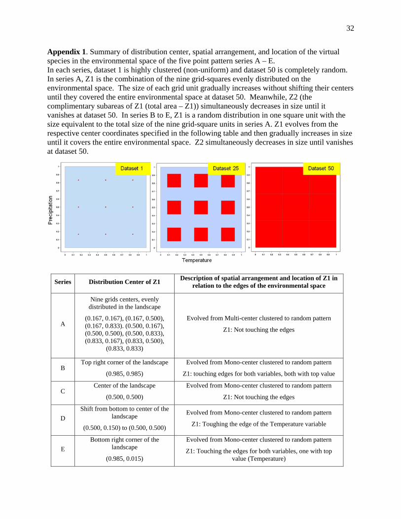
Appendix 1. Summary of distribution center, spatial arrangement, and location of the virtual species in the environmental space of the five point pattern series A – E. In each series, dataset 1 is highly clustered (non-uniform) and dataset 50 is completely random. In series A, Z1 is the combination of the nine grid-squares evenly distributed on the environmental space. The size of each grid unit gradually increases without shifting their centers until they covered the entire environmental space at dataset 50. Meanwhile, Z2 (the complimentary subareas of Z1 (total area – Z1)) simultaneously decreases in size until it vanishes at dataset 50. In series B to E, Z1 is a random distribution in one square unit with the size equivalent to the total size of the nine grid-square units in series A. Z1 evolves from the respective center coordinates specified in the following table and then gradually increases in size until it covers the entire environmental space. Z2 simultaneously decreases in size until vanishes at dataset 50.
Series Distribution Center of Z1 Description of spatial arrangement and location of Z1 in
relation to the edges of the environmental space
A
Nine grids centers, evenly distributed in the landscape
(0.167, 0.167), (0.167, 0.500), (0.167, 0.833). (0.500, 0.167), (0.500, 0.500), (0.500, 0.833), (0.833, 0.167), (0.833, 0.500),
(0.833, 0.833)
Evolved from Multi-center clustered to random pattern
Z1: Not touching the edges
B Top right corner of the landscape
(0.985, 0.985)
Evolved from Mono-center clustered to random pattern
Z1: touching edges for both variables, both with top value
C Center of the landscape
(0.500, 0.500)
Evolved from Mono-center clustered to random pattern
Z1: Not touching the edges
D
Shift from bottom to center of the landscape
(0.500, 0.150) to (0.500, 0.500)
Evolved from Mono-center clustered to random pattern
Z1: Toughing the edge of the Temperature variable
E
Bottom right corner of the landscape
(0.985, 0.015)
Evolved from Mono-center clustered to random pattern
Z1: Touching the edges for both variables, one with top value (Temperature)
33
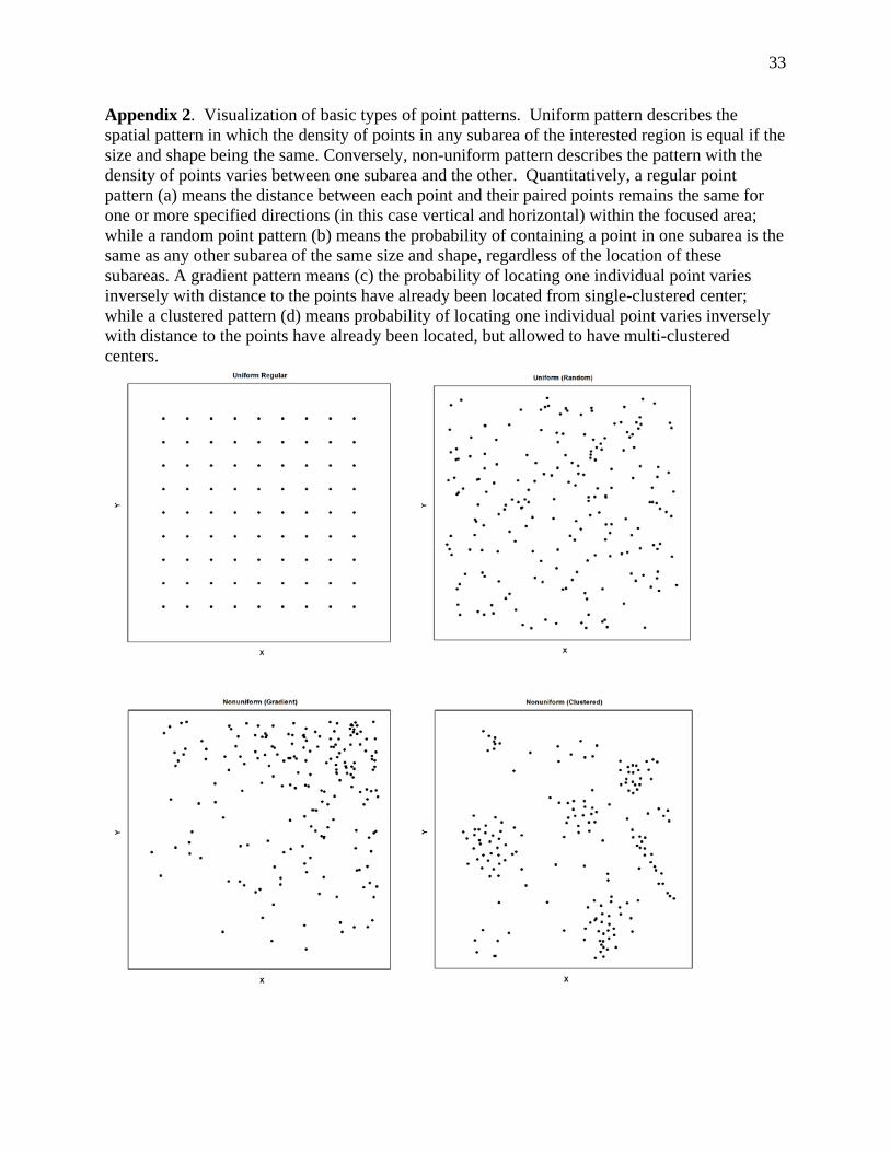
Appendix 2. Visualization of basic types of point patterns. Uniform pattern describes the spatial pattern in which the density of points in any subarea of the interested region is equal if the size and shape being the same. Conversely, non-uniform pattern describes the pattern with the density of points varies between one subarea and the other. Quantitatively, a regular point pattern (a) means the distance between each point and their paired points remains the same for one or more specified directions (in this case vertical and horizontal) within the focused area; while a random point pattern (b) means the probability of containing a point in one subarea is the same as any other subarea of the same size and shape, regardless of the location of these subareas. A gradient pattern means (c) the probability of locating one individual point varies inversely with distance to the points have already been located from single-clustered center; while a clustered pattern (d) means probability of locating one individual point varies inversely with distance to the points have already been located, but allowed to have multi-clustered centers.

34
Appendix 3 . Binned calibration method. Red line corresponds to the perfect calibration of the model, when the plotted points fall on the 1:1 line. The coefficient of the regression line (black) represents the overall calibration of each run from the individual datasets (1 to 50) of each series
35
Appendix 4 Point patterns of species occurrence data in the extracted environmental space (from the native range) for Prosopis farcta (A) and Imperata cylindrica (B), represented by the component scores of the dimension reduction results of PCA. Red dots represent the occurrence data locations reflected in the environmental space. Boundaries of the environmental space correspond to their environmental space within the native ranges. The extents of the environmental space reflect the relative size of the native ranges for these two species
2.862