RIGHT:

URL:

CITATION:

AUTHOR(S):

ISSUE DATE:

TITLE:

Numerical simulation of Faradaywaves oscillated by two-frequencyforcing

Takagi, Kentaro; Matsumoto, Takeshi

Takagi, Kentaro ...[et al]. Numerical simulation of Faraday wavesoscillated by two-frequency forcing. Physics of Fluids 2015, 27(3):032108.

2015-03-24

http://hdl.handle.net/2433/216144

© 2015 AIP Publishing LLC. This article may be downloaded for personal use only. Anyother use requires prior permission of the author and AIP Publishing. The following articlemay be found athttp://scitation.aip.org/content/aip/journal/pof2/27/3/10.1063/1.4915340

Numerical simulation of Faraday waves oscillated by two-frequency forcingKentaro Takagi and Takeshi Matsumoto Citation: Physics of Fluids (1994-present) 27, 032108 (2015); doi: 10.1063/1.4915340 View online: http://dx.doi.org/10.1063/1.4915340 View Table of Contents: http://scitation.aip.org/content/aip/journal/pof2/27/3?ver=pdfcov Published by the AIP Publishing Articles you may be interested in Low-frequency vortex oscillation around slender bodies at high angles-of-attack Phys. Fluids 26, 091701 (2014); 10.1063/1.4895599 Aspect ratio and radius ratio dependence of flow pattern driven by differential rotation of acylindrical pool and a disk on the free surface Phys. Fluids 25, 084101 (2013); 10.1063/1.4817179 Pattern formation in a reaction-diffusion-advection system with wave instability Chaos 22, 023112 (2012); 10.1063/1.4704809 Three-dimensional numerical study of natural convection in vertical cylinders partially heated fromthe side Phys. Fluids 17, 124101 (2005); 10.1063/1.2141430 Large-eddy simulation of low frequency oscillations of the Dean vortices in turbulent pipe bendflows Phys. Fluids 17, 035107 (2005); 10.1063/1.1852573

This article is copyrighted as indicated in the article. Reuse of AIP content is subject to the terms at: http://scitation.aip.org/termsconditions. Downloaded

to IP: 130.54.110.72 On: Fri, 24 Apr 2015 00:32:37

A Self-archived copy inKyoto University Research Information Repository

https://repository.kulib.kyoto-u.ac.jp

PHYSICS OF FLUIDS 27, 032108 (2015)

Numerical simulation of Faraday waves oscillatedby two-frequency forcing

Kentaro Takagia) and Takeshi Matsumotob)

Division of Physics and Astronomy, Graduate School of Science, Kyoto University,Kitashirakawa Oiwaketyo, Sakyoku, Kyoto 606-8502, Japan

(Received 19 September 2014; accepted 14 February 2015; published online 24 March 2015)

We perform a numerical simulation of Faraday waves forced with two-frequencyoscillations using a level-set method with Lagrangian-particle corrections (particlelevel-set method). After validating the simulation with the linear stability analysis,we show that square, hexagonal, and rhomboidal patterns are reproduced in agree-ment with the laboratory experiments [Arbell and Fineberg, “Two-mode rhomboidalstates in driven surface waves,” Phys. Rev. Lett. 84, 654–657 (2000) and “Tempo-rally harmonic oscillons in Newtonian fluids,” Phys. Rev. Lett. 85, 756–759 (2000)].We also show that the particle level-set’s high degree of conservation of volumeis necessary in the simulations. The numerical results of the rhomboidal states arecompared with weakly nonlinear analysis. Difficulty in simulating other patterns ofthe two-frequency forced Faraday waves is discussed. C 2015 AIP Publishing LLC.[http://dx.doi.org/10.1063/1.4915340]

I. INTRODUCTION

Faraday waves,1 known to exhibit various kinds of crystalline patterns in simple settings, haveattracted many researchers for about two hundred years. Faraday waves are the surface waves betweentwo superposed immiscible fluid layers subjected to a vertical vibration. Even recently astoundingexotic phenomena continue to be found in laboratory experiments on Faraday waves. For example, inFaraday waves with a certain non-Newtonian fluid (shear-thickening fluid), the behavior of the inter-face is far beyond what one can imagine from the interface motion between air and water.2 In anothersurprising experiment, a droplet slightly submerged in a liquid substrate under a vertical oscillationis found to behave dynamically like a snake.3 To physically understand these phenomena, numericalsimulations of them, which may not be possible now, are expected to play a decisive role.

As a first step to build such numerical methods, we here study numerically Faraday waves sub-jected to a two-frequency forcing in a Newtonian fluid. There are a number of experimental resultswith this forcing setting,4–13 where much richer variations of the selected patterns are found than inthe single-frequency forced cases as listed below.

The study of two-frequency forced Faraday waves starts with the experiments by Edwards andFauve4,5 and Muller.6 The two-frequency forcing can be written as A1 cos(mω0t) + A2 cos(nω0t + φ)and characterized by the integers m and n. Edwards and Fauve explored various ratios of the twofrequencies such as m:n = 3:5, 4:5, 6:7, 4:7, and 8:9 and mainly investigated the ratio 4:5. Theyobserved the quasi-pattern, which has a long-range orientational order but no spatial periodicity. Onthe other hand, the experiment by Muller is focused on the driving ratio of 1:2 and produces a trian-gular pattern.

In the linear regime of the two-frequency forced case, a bicritical point exists at which two normalmodes with different wavenumber moduli become simultaneously unstable (for the single-frequencyforced case, the bicritical point can be formed by tuning the frequency of the forcing for shallowlayers14). The unstable modes then interact with each other nonlinearly. In the neighborhood of the

a)Electronic mail: kentaro@kyoryu.scphys.kyoto-u.ac.jpb)Electronic mail: takeshi@kyoryu.scphys.kyoto-u.ac.jp

1070-6631/2015/27(3)/032108/21/$30.00 27, 032108-1 ©2015 AIP Publishing LLC

This article is copyrighted as indicated in the article. Reuse of AIP content is subject to the terms at: http://scitation.aip.org/termsconditions. Downloaded

to IP: 130.54.110.72 On: Fri, 24 Apr 2015 00:32:37

A Self-archived copy inKyoto University Research Information Repository

https://repository.kulib.kyoto-u.ac.jp

032108-2 K. Takagi and T. Matsumoto Phys. Fluids 27, 032108 (2015)

bicritical point, many complex patterns are expected to be found. A number of experiments aroundthe bicritical point were conducted by Kudrolli et al.,7 Arbell and Fineberg ,8–11 and Epstein andFineberg.12,13 Kudrolli et al. observed patterns that they named superlattice-1 and superlattice-2. Ar-bell and Fineberg and Epstein and Fineberg observed double hexagonal superlattice (DHS), subhar-monic superlattice states (SSS), oscillon, two-mode superlattices (2MS), and 2k rhomboidal states(2kR). Each pattern can be characterized by the number of excited (discrete) Fourier modes and bythe nonlinear resonance among them.

To the best of our knowledge, numerical simulation of the two-frequency forced Faraday wavesbased on the Navier-Stokes equations solving the motion of both the top and bottom fluids is reportedin this paper for the first time. However, such a simulation, not limited to the two-frequency forcedcase, requires treatment of the interface with the surface tension force. We therefore must employ oneof the interface-tracking schemes such as the volume-of-fluid methods, the level-set methods, andthe front-tracking methods (see, e.g., an advanced textbook15). In this study, we adopt the level-setmethod and investigate whether or not the simulation of two-frequency forced Faraday waves withthe level-set method is consistent with the experimental results. The reason for adopting the level-setmethod will be described later.

The first numerical simulation of the single-frequency forced Faraday waves in three dimen-sions was performed by Périnet et al.,16 who reproduced the square and hexagonal patterns in quan-titative agreement with the laboratory experiment by Kityk et al.17 Périnet et al.16 used a front-tracking method. It is necessary, for example, in simulating oscillon or snake-like patterns, to allowfor overturning and topological change of the interface. We hence believe that other interface-trackingschemes should be explored and tested for a wider class of the Faraday waves. Another numericalissue concerns the density difference between the top and the bottom fluids. In typical laboratoryexperiments, these are air and water at room temperature, meaning three orders of magnitude differ-ence in the densities. To handle this large difference, it is known that a high quality solver for thepressure Poisson equation is needed regardless of the choice of interface-tracking scheme.15 We usea preconditioned BiCGSTAB.

On the theoretical front of the two-frequency forced Faraday waves, linear stability analysis andweakly nonlinear theory are available. Linear analysis was performed by Besson and Edwards,18

which is an extension of the single-frequency forced case.19 Their results18 agree with the experimentsquantitatively. In the weakly nonlinear analysis, whose emphasis is on the pattern selection of thetwo-frequency Faraday waves, Silber et al., Tse et al., Porter et al., and Topaz et al.20–26 formulatedan amplitude equation up to third order in amplitude by applying symmetry based arguments.

By analyzing the structure of the three-wave resonance, they succeeded in explaining manyselected patterns qualitatively. Quantitative prediction of the pattern can be obtained if the amplitudeequation of the two-frequency forced Faraday waves is derived from the Navier-Stokes equation witha realistic boundary condition. However this is a formidable task. A reduced hydrodynamic equationof the two-frequency Faraday waves was derived by Zhang and Viñals.27 From this reduced equation,the amplitude equations are derived and analyzed by assuming infinite depth and small viscosity.25–27

Weakly nonlinear analysis based on the Navier-Stokes equations with infinite depth was carried out bySkeldon and Guidoboni.28 This approach with realistic amplitude equations is successful in explainingmany patterns observed in the two-frequency forced Faraday waves. Nevertheless, there are some pat-terns, such as oscillons,10 which are not explained so far by the weakly nonlinear analysis. In the effortto understand these patterns, numerical simulation of the Faraday waves plays a complementary role.

For this reason, we develop a method of numerical simulation of the two-frequency forced Fara-day waves, which is consistent with the experiments. Specifically, we here simulate three patternsobserved in the experiments by Arbell and Fineberg.9,10 In particular, the rhomboidal pattern does notappear in the single-frequency forced Faraday waves. In order to validate the simulations, we compareour results with the linear stability analysis of two frequency Faraday waves.18 Next, in the nonlinearregime, we reproduce the square pattern and the hexagonal pattern with the same physical parametersas the respective experiments. After that we reproduce and study the rhomboidal state. During thesimulations, we compare two kinds of level-set methods: one is the original implementation29,30 andthe other is the level-set method with Lagrangian particles (particle level-set method).31 Finally, wediscuss the difficulty of simulating other patterns observed in the experiments.

This article is copyrighted as indicated in the article. Reuse of AIP content is subject to the terms at: http://scitation.aip.org/termsconditions. Downloaded

to IP: 130.54.110.72 On: Fri, 24 Apr 2015 00:32:37

A Self-archived copy inKyoto University Research Information Repository

https://repository.kulib.kyoto-u.ac.jp

032108-3 K. Takagi and T. Matsumoto Phys. Fluids 27, 032108 (2015)

The organization of the paper is the following. In Sec. II, we describe the fluid dynamical equa-tions of the Faraday waves, the two level-set methods, and numerical discretization of the equations.The numerical results are presented in Sec. III. More specifically, comparisons of the simulation withthe linear analysis and simple patterns such as square and hexagonal patterns are presented in Secs.III A and III B. The simulation of the rhomboidal states is shown in Sec. III C. In Sec. III D, wecompare the original level-set method and the particle level-set method. Our summary and discussionare in Sec. IV.

II. EQUATIONS AND NUMERICAL METHOD

In this section, we describe our numerical method for the governing equations and the boundaryconditions used for simulating Faraday waves oscillated by the two-frequency forcing.

A. Navier-Stokes equations

Faraday waves occur on the interface between an upper and a lower immiscible fluids. We employthe one-fluid description of the problem. Numerically, we simulate the dynamics in both fluid layers.The incompressible Navier-Stokes equations are written as

∇ · u = 0, (1)

ρDtu = −∇p + ρG + ∇ · η(∇u + ∇uT) + s. (2)

Here, Dt,p,and u are the material derivative, the pressure, and the velocity, respectively, and s, ρ, andη are the surface force, the density, and the viscosity, respectively. The vector G is the gravitationalterm in the reference frame of the container,

G = (−g + A1 cos(mω0t) + A2 cos(nω0t + θ))ez, (3)

where g, A1, A2, ω0, θ,and ez are the gravitational acceleration, the amplitude of the first periodicforcing, the amplitude of the second periodic forcing, the base angular frequency of the periodic forc-ing, the phase shift between the two modes, and the unit vector in the vertical z-direction, respectively.In this paper, we set the integers m and n to 2 and 3. We also use the notationsω1 = mω0 = 2ω0, ω2 =

nω0 = 3ω0.On the top and bottom boundaries, no-slip boundary conditions are assumed. For the horizontal

direction, we assume periodic boundary conditions. The interface location z = ζ(x, y, t) obeys thekinematic boundary condition. In term of this ζ , the density ρ and η are written as

(ρ,η) =

(ρt, ηt), z > ζ(x, y, t),(ρb, ηb), z ≤ ζ(x, y, t), (4)

where ρt, ηt are the density and the viscosity of the top fluid and ρb, ηb are the density and theviscosity of the bottom fluid.

In this sharp interface description, the density and the viscosity change discontinuously at thedynamically evolving interface. This situation is a challenge for numerical simulations. To circumventthis difficulty, various numerical methods have been proposed, such as the volume-of-fluid methods,the level-set methods, and the front-tracking methods, just to name a few.15,32 In this study, we adoptthe level-set method. The reason is as follows. The level-set method has a high numerical accuracy ofthe normal vector and the curvature of the interface, hence adequate for the gravity-capillary waves.However, it is well known that the level-set method does not have good mass conservation prop-erties.32 A number of improvements have been proposed.30–33 Among them, we use the level-setmethod corrected with Lagrangian particles, the so-called particle level-set method, to ensure volumeconservation.31 This conservation problem is discussed in detail in Sec. III D.

In the following Sec. II B, we describe the level-set method without the particles; here, we callthe original level-set method and the particle level-set method and their numerical discretizations.The description of the discretization of the Navier-Stokes equations follows later.

This article is copyrighted as indicated in the article. Reuse of AIP content is subject to the terms at: http://scitation.aip.org/termsconditions. Downloaded

to IP: 130.54.110.72 On: Fri, 24 Apr 2015 00:32:37

A Self-archived copy inKyoto University Research Information Repository

https://repository.kulib.kyoto-u.ac.jp

032108-4 K. Takagi and T. Matsumoto Phys. Fluids 27, 032108 (2015)

B. Level-set method

1. Level-set function

We use the level-set approach29 to describe the interface motion. Here, the level-set functionφ(x, t), the signed distance from the interface, indicates the interface. We define φ > 0 in the top fluidand φ < 0 in the bottom fluid. The level-set function obeys the following equation:

∂tφ + (u · ∇)φ = 0, (5)

which is discretized with the 5th-order weighted essentially non-oscillatory (WENO) scheme34 andintegrated in time through the 3rd-order total variation diminishing (TVD) Runge-Kutta method.34

2. Reinitialization of level-set function

It is known that the analytic integration of Eq. (5) does not ensure that φ(x, t) is the signed dis-tance function from the interface. By definition, being the signed distance function requires |∇φ| = 1.However, this unit gradient condition is not satisfied since the Lagrange derivative of |∇φ|2 is notzero but Dt |∇φ|2 = −2(∇φ)(∇u)(∇φ). To enforce the condition (in practice, we do so just around theinterface), the distance function is re-initialized at each time step from the following initial valueproblem with the virtual time τ:30

∂d∂τ= sgn(φ)(1 − |∇d |) + λ f (φ), (6)

d(x, y, z, τ = 0) = φ(x, y, z).Although we call τ virtual time, its dimension is length. Ideally, the function d(x, τ) as τ → ∞ givesthe corrected signed distance function for all the computational domain. Here, we set φ(x, t) = d(x, τ =τl) for some value τl. This τl corresponds to the largest distance from the interface to which we demandφ be the signed distance. In this paper, we use τl = ϵ , where ϵ is the half-width of the diffuse interfaceand set to 2∆z, where ∆z is the grid spacing in the vertical z-direction. The functions λ(x), f (φ) inEq. (6) are given as

λ(x) = −Ω(x) H ′(φ)L(φ,d)dxΩ(x) H ′(φ) f (φ)dx

, (7)

f (φ) = H ′(φ)|∇φ|, (8)

H ′(φ) = dHdφ

, (9)

H(φ) =

0, if φ < −ϵ,121 +

φ

ϵ+

1π

sin(πφϵ), if − ϵ ≤ φ ≤ ϵ,

1, if φ > ϵ,

(10)

where Ω(x) is a small region centered at the point x, L(φ,d) = sgn(φ)(1 − |∇d |), ϵ = 2∆z is the pre-scribed interface width, H(φ) is the smoothed Heaviside function, and H ′(φ) is the smoothed deltafunction.

Numerically, the reinitialization is done in the following way. First, we ignore the term λ(x) f (φ)in the Eq. (6) and solve

∂d∂τ= sgn(φ)(1 − |∇d |), (11)

where the discretization in space is the same as that of Eq. (5). The integration in the virtual time isdiscretized as follows

This article is copyrighted as indicated in the article. Reuse of AIP content is subject to the terms at: http://scitation.aip.org/termsconditions. Downloaded

to IP: 130.54.110.72 On: Fri, 24 Apr 2015 00:32:37

A Self-archived copy inKyoto University Research Information Repository

https://repository.kulib.kyoto-u.ac.jp

032108-5 K. Takagi and T. Matsumoto Phys. Fluids 27, 032108 (2015)

d ′ = dn + ∆τL(φ,dn), (12)

d∗ =14(3dn + d ′ + ∆τL(φ,d ′)), (13)

d ′n+1 =13(dn + 2(d∗ + ∆τL(φ,d∗))), (14)

where ∆τ = 0.5 min(∆x,∆y,∆z).Second, we calculate λ(x) according to the following equation:

λi jk =−Ωi jk

H ′(φ) d′n+1−φ∆τ

dxΩi jk

H ′(φ) f (φ)dx. (15)

Here, λi jk denotes λ(xi jk) on the grid point xi jk specified by the index (i, j, k). The integral rangeΩi jk

describes the cell region associated with the grid point. For the three dimensional case, by followingthe two-dimensional version,35 we discretize the integral of some function g(x) in the cell as

Ωi jk

g(x) dx =∆x∆y∆z

1512[9(gi+1, j+1,k + gi+1, j−1,k

+gi−1, j+1,k + gi−1, j−1,k + gi, j+1,k+1

+gi, j+1,k−1 + gi, j−1,k+1 + gi, j−1,k−1

+gi+1, j,k+1 + gi+1, j,k−1 + gi−1, j,k+1

+gi−1, j,k−1) + 88(gi+1, j,k + gi−1, j,k

+gi, j+1,k + gi, j−1,k + gi, j,k+1

+gi, j,k−1) + 876gi, j,k], (16)

where ∆x,∆y,∆z are the grid spacings along the x, y, z directions.Finally, dn+1 is calculated by

dn+1 = d ′n+1 + ∆τλi jkH ′(φ)|∇φ|. (17)

In practice, we take the total number of the virtual time steps as τl/∆τ ≃ 4.

C. Particle level-set method

In order to improve the volume conservation of the level-set method, it has been proposed toutilize Lagrangian information to correct the level-set function by adding marker particles near theinterface. Our procedure of the particle level-set method is basically the same as that of Enrightet al.31 The differences are in the error correction and the reseeding strategy.

1. Initialization of particles

The marker particles are spread in the neighborhood of the interface, in which |φ| < 3 max(∆x,∆y,∆z) is satisfied. The number of particles in each cell is set to 64. A marker particle has signsp = 1 or −1 and the radius rp. There are a number of strategies for setting the sign and radius. Onesimple strategy is to set the sign to that of the level-set function at the particle and the radius to theabsolute value of the level-set function. However, we follow the more sophisticated strategy proposedby Enright et al. to improve numerical results.

The strategy is as follows. Initially, the particle’s sign is set randomly. In order to have the samesign between the particle and the level-set function, the particles at xp, (p = 1,2,3, . . .) are iterativelymoved by the following recurrence relation:

xn+1p = xn

p + 2−n(φgoal − φ(xn))N(xnp), (18)

where N(xnp) = ∇φ(xnp)

|∇φ(xnp)| is the normal vector. Here, φgoal is set as follows. The sign, sgn(φp), isset to have the same as that of the particle sp. In addition, the absolute value is chosen to be a

This article is copyrighted as indicated in the article. Reuse of AIP content is subject to the terms at: http://scitation.aip.org/termsconditions. Downloaded

to IP: 130.54.110.72 On: Fri, 24 Apr 2015 00:32:37

A Self-archived copy inKyoto University Research Information Repository

https://repository.kulib.kyoto-u.ac.jp

032108-6 K. Takagi and T. Matsumoto Phys. Fluids 27, 032108 (2015)

uniformly distributed random variable in the range bmin < |φgoal| < bmax. In this study, bmin is setto 0.1 min(∆x,∆y,∆z) and bmax is set to 3 max(∆x,∆y,∆z). Each particle is moved repeatedly byEq. (18) until it satisfies the condition bmin < spφ(xp) < bmax. Finally, each particle radius is setaccording to

rp =

ru spφ(xp) > ru,spφ(xp) rl < spφ(xp) < ru,rl spφ(xp) < rl,

(19)

where rl and ru are lower and upper limits of particle radius to prevent the creation of particleswhich are too small or too large. We use rl = 0.1 min(∆x,∆y,∆z) and ru = 5rl. The particle radiusrp is used to correct the level-set function later. After this procedure, the positive particles at positionxp are in the φ(xp) > 0 side (the top fluid) and the negative particles are in the φ(xp) < 0 side (thebottom fluid). The envelope formed by the circles of the same-sign particles coincides with theinterface φ = 0.

2. Advection of particles

Each particle at position xp(t) is advected by

dxp(t)dt

= u(xp(t), t). (20)

The velocity at the particle position u(xp(t), t) is calculated with trilinear interpolation from the ve-locity vectors on the nearby cell faces. The 3rd order TVD Runge-Kutta method is used to integrateEq. (20) in time.

3. Error correction of level-set function

As a result of the advection Eq. (20), some particles move across the interface φ = 0. Suchescaped particles are used to correct the level-set function φ in the following manner. First, particlesplaced on the wrong side (φ(xp) × sp < 0) are considered to have escaped. Second, we introduce thesigned distance function between the escaped particle and a point x, which is calculated with theparticle radius rp as

φp(x) = sp(rp − |x − xp |). (21)

This signed distance is positive (φp(x) > 0) if the point x is within the positive ball (sp = 1) ofradius rp centered on xp. The distance function corrected by the escaped positive (negative) particleφ+(x) (φ−(x)) is calculated from

φ+(x) = max∀p∈E+

(φp, φ(x)), (22)

φ−(x) = min∀p∈E−

(φp, φ(x)). (23)

Here, E+ and E− denote the sets of the escaped positive and negative particles. Finally, the level-setfunction φ(x) is corrected as

φ(x) =

φ+(x) if |φ+(x)| ≤ |φ−(x)|,φ−(x) if |φ−(x)| < |φ+(x)|. (24)

Ideally, after this correction of the distance function, all the particles tagged as escaped have thesame sign as the corrected distance function. However, with our implementation of the correction inthe preliminary calculations, we find that some particles do not have the same sign of the correcteddistance function. If we use such particles with the wrong sign in the next correction process, theinterface becomes nearly singular, which we consider a numerical artifact. Therefore, we ignore suchescaped particles in the later correction processes. The point differs from the usual procedure of theparticle level-set method.31

This article is copyrighted as indicated in the article. Reuse of AIP content is subject to the terms at: http://scitation.aip.org/termsconditions. Downloaded

to IP: 130.54.110.72 On: Fri, 24 Apr 2015 00:32:37

A Self-archived copy inKyoto University Research Information Repository

https://repository.kulib.kyoto-u.ac.jp

032108-7 K. Takagi and T. Matsumoto Phys. Fluids 27, 032108 (2015)

4. Reseeding of particles

Generally, as a result of advection of the particles by a flow, some regions lack sufficient particlesto correct the level-set function. We reseed the particles where needed. Specifically, in the cells nearthe interface (|φ(x)| ≤ bmax), we keep the number of particles in a cell to 64 by adding particles forcells which particles exit or deleting particles for cells which particles enter. In our simulation, thereseeding procedure is executed with the following two strategies. The first strategy is that the reseed-ing is done after 40 time steps from the previous reseeding. The second strategy is that the reseedingis done when the surface area of the interface increases by 30% after the previous reseeding time.The surface area is calculated from

A =

δ(φ)|∇φ|dx, (25)

δ(φ) =

0, |φ| > ϵ,12ϵ

(1 + cos(πφ

ϵ)), |φ| ≤ ϵ,

(26)

where the smoothed delta function δ(φ) is the same as H ′(φ) of Eq. (9).In summary, the one-step update of the level-set function with particles is carried out by the

following steps.31

1. The level-set function is advected by Eq. (5).2. The particles are advected by Eq. (20).3. The error of the level-set function is corrected by the procedure described in the Sec. II C 3.4. The level-set function is reinitialized as described in Sec. II B 2.5. The error of the level-set function is once more corrected by the particles as described in Sec.

II C 3.

For the original level-set method without particles, the second, third, and fifth processes are omitted.

D. Discretization of Navier-Stokes equations

We use the following temporal discretization of incompressible Navier-Stokes Eqs. (1) and (2)with the projection method and with adaptive time stepping:

u∗ = un + ∆tn

−(1 +∆tn−1

∆tn

)An +

∆tn−1

∆tnAn−1

+

(1 +∆tn−1

∆tn

)Dn

e −∆tn−1

∆tnDn−1

e

+12D∗i + Dn

i

+ Gn + Sn+1

, (27)

un+1 = u∗ + ∆tn1ρn∇pn+1. (28)

Here, the superscript n denotes the value at the n-th time step tn =n

i=1∆t i in which ∆t i is the timestep size for the i-th step. We discuss later how to determine them. An is the advective term, Dn

i and D∗iare the viscous terms involving the same component as on the left-hand-side and at the intermediatestep, Dn

e is the viscous term involving the other components, Gn is gravity, and Sn is the surface forceterm. Here, by ∗, we denote the intermediate step. As in the standard way of the projection method,the pressure term pn+1 is calculated from the divergence free condition. Equation (28) acted upon by∇· becomes

− ∇u∗

∆tn= ∇

(1ρn∇pn+1

). (29)

This article is copyrighted as indicated in the article. Reuse of AIP content is subject to the terms at: http://scitation.aip.org/termsconditions. Downloaded

to IP: 130.54.110.72 On: Fri, 24 Apr 2015 00:32:37

A Self-archived copy inKyoto University Research Information Repository

https://repository.kulib.kyoto-u.ac.jp

032108-8 K. Takagi and T. Matsumoto Phys. Fluids 27, 032108 (2015)

The advection term An is described by

An = un · ∇un. (30)

The x-component of the viscous term Dni to be treated implicitly is

Dnix =

1ρn

∇ (ηn∇un

x) + ∂

∂x

(ηn ∂un

x

∂x

). (31)

The viscous term D∗i x is defined similarly but with the intermediate velocity u∗. The x-component ofthe viscous term Dn

e to be treated explicitly is

Dnex =

1ρn

∂

∂ y

(ηn

∂uny

∂x

)+

∂

∂z

(ηn

∂unz

∂x

). (32)

Other components of the viscous terms are described in the same manner. The gravitational term Gn

is

Gn = (−g + A1 cos(ω1tn) + A2 cos(ω2tn + θ))ez. (33)

The surface force term Sn is

Sn = σκnnn, nn =∇φn

|∇φn | , κn = ∇ · nn. (34)

Regarding the spacial discretizations, the advection term, An,is discretized with the 2nd-order essen-tially non-oscillatory (ENO) scheme. The other derivative terms in D∗i ,D

ni ,D

ne ,nn, κn are discretized

with the 2nd-order central difference scheme.Concerning the boundary conditions, we assume periodic boundary conditions in the horizontal

directions (x and y directions). For the vertical z direction, we assume the non-slip condition atz = 0,Lz,

u|z=0, Lz = 0. (35)

The boundary condition for the pressure in solving Poisson equation (29) is

∂p∂z

z=0, Lz

= 0. (36)

For calculating u∗ in Eq. (27), the localized incomplete LU (ILU) factorization preconditioned bicon-jugate gradient stabilized (BiCGSTAB) method36 is adopted and the Poisson equation of the pressureis solved by the multigrid preconditioned BiCGSTAB method.36

Finally, we describe how we determine the variable time step size ∆t i which is determined by

∆t i = c minx(∆tS, ∆t if (x), ∆tη(x), ∆t ic f l(x)), (37)

where we set the safety constant c = 0.40. Here, ∆tS, ∆t f , and ∆tη are the time scales of surfaceforce, the vertical vibration, and the viscosity, respectively. The time scale∆tc f l concerns the Courant-Friedrichs-Lewy (CFL) condition. These reference time scales are defined as

∆tS =

(ρt + ρb)dh3

4πσ, (dh = min(∆x,∆y,∆z)), (38)

∆t if (x) =

dhGi · ez

, ∆tη(x) = ρ

η

11∆x2 +

1∆y2 +

1∆z2

, (39)

∆t ic f l(x) =1

uix∆x+

uiy∆y+

uiz∆z

. (40)

Typically, ∆tS is the smallest in our all simulations.

This article is copyrighted as indicated in the article. Reuse of AIP content is subject to the terms at: http://scitation.aip.org/termsconditions. Downloaded

to IP: 130.54.110.72 On: Fri, 24 Apr 2015 00:32:37

A Self-archived copy inKyoto University Research Information Repository

https://repository.kulib.kyoto-u.ac.jp

032108-9 K. Takagi and T. Matsumoto Phys. Fluids 27, 032108 (2015)

III. NUMERICAL RESULTS

Our goal in this paper is numerical simulation of the 2k rhomboidal states observed in thelaboratory experiments by Arbell and Fineberg9,10 To the best of our knowledge, the rhomboidalstates have not previously been obtained in numerical simulations of the Navier-Stokes equations.In particular, we use the same bulk fluid parameters as the experiments. The only difference is thegeometry of the system, i.e., the domain size and the boundary conditions. In the simulations, weapply periodic boundary conditions in the horizontal directions, with which we can reduce numericalcost by not simulating many repeated patterns in the computational domain. While the experimentsare conducted in an open container, we assume the presence of a rigid wall above the top fluid, onwhich the no-slip boundary condition is applied. This setting is numerically easier than simulatingthe top-fluid motion in a semi-infinite domain. We assume that the top-fluid height is four timeslarger than the bottom-fluid depth.

Before presenting the simulation, we first describe the validation of our fully nonlinear simu-lation with the above mentioned geometry by comparing with the linear stability analysis oftwo-frequency forced Faraday waves.18 This validation process is the same as Périnet et al.16

The second test then is to reproduce the square and hexagonal patterns observed in the sametwo-frequency forced experiments.9,10 A direct numerical simulation of the square and hexagonpatterns for the single-frequency forced Faraday waves is performed by Périnet et al.16,37 The resulton the rhomboidal states is presented after the validations.

A. Comparison with linear stability analysis

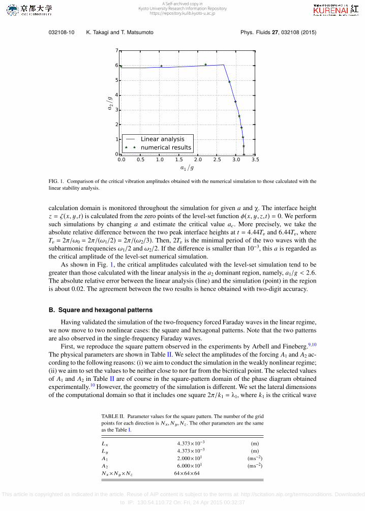
We now compare the critical amplitudes of the oscillations calculated with the fully nonlinearnumerical simulation with those calculated with the linear stability analysis. We write the two-frequency forcing as a(cos(χ) cos(ω1t) + sin(χ) cos(ω2t + θ)). In the linear analysis, once we fix thephysical parameters as shown in Table I and the mixing angle χ, the critical value of a, denotedas ac, and the associated critical wave number can be calculated.18,19 Here, we assume that eitherharmonic frequency (ω1,ω2) or sub-harmonic frequency (ω1/2,ω2/2) gives the lowest critical value.The critical amplitudes a1c = ac cos(χ) and a2c = ac sin(χ) for the mixing angle χ from 0 to 90 areshown as the solid line in Fig. 1.

Meanwhile, with the particle level-set simulation, we determine the critical amplitudes byadding small perturbations to basic modes for ten different values of the mixing angle, χ =0,10,20, . . . ,90. The results are denoted as points in Fig. 1. The way to estimate the criticalamplitudes a1c and a2c in the nonlinear simulation is as follows: (i) the perturbation is added tothe normal mode whose wavenumber is set to the critical wave number (kc) calculated from thelinear analysis. More precisely, the perturbation, ξ sin(kcx), is added to the flat interface, where theperturbation amplitude ξ is set to 2 × 10−2Lz. (ii) the interface height ζ(x, y, t) at the center of the

TABLE I. Parameter values for the linear stability analysis. These param-eters (except for Lz and θ) are identical to the experiment by Arbell andFineberg.10

ρt 1.293 (kgm−3)ρb 9.500×102 (kgm−3)ηt 1.822×10−5 (kgm−1s−1)ηb 2.185×10−2 (kgm−1s−1)ω1= 2ω0 3.770×102 (s−1)ω2= 3ω0 5.655×102 (s−1)θ 0 (rad)σ 2.150×10−2 (kgm−1)g 9.807 (ms−2)Lz 1.00×10−2 (m)Bottom-fluid depth 2.00×10−3 (m)

This article is copyrighted as indicated in the article. Reuse of AIP content is subject to the terms at: http://scitation.aip.org/termsconditions. Downloaded

to IP: 130.54.110.72 On: Fri, 24 Apr 2015 00:32:37

A Self-archived copy inKyoto University Research Information Repository

https://repository.kulib.kyoto-u.ac.jp

032108-10 K. Takagi and T. Matsumoto Phys. Fluids 27, 032108 (2015)

FIG. 1. Comparison of the critical vibration amplitudes obtained with the numerical simulation to those calculated with thelinear stability analysis.

calculation domain is monitored throughout the simulation for given a and χ. The interface heightz = ζ(x, y, t) is calculated from the zero points of the level-set function φ(x, y, z, t) = 0. We performsuch simulations by changing a and estimate the critical value ac. More precisely, we take theabsolute relative difference between the two peak interface heights at t = 4.44Tv and 6.44Tv, whereTv = 2π/ω0 = 2π/(ω1/2) = 2π/(ω2/3). Then, 2Tv is the minimal period of the two waves with thesubharmonic frequencies ω1/2 and ω2/2. If the difference is smaller than 10−3, this a is regarded asthe critical amplitude of the level-set numerical simulation.

As shown in Fig. 1, the critical amplitudes calculated with the level-set simulation tend to begreater than those calculated with the linear analysis in the a2 dominant region, namely, a1/g < 2.6.The absolute relative error between the linear analysis (line) and the simulation (point) in the regionis about 0.02. The agreement between the two results is hence obtained with two-digit accuracy.

B. Square and hexagonal patterns

Having validated the simulation of the two-frequency forced Faraday waves in the linear regime,we now move to two nonlinear cases: the square and hexagonal patterns. Note that the two patternsare also observed in the single-frequency Faraday waves.

First, we reproduce the square pattern observed in the experiments by Arbell and Fineberg.9,10

The physical parameters are shown in Table II. We select the amplitudes of the forcing A1 and A2 ac-cording to the following reasons: (i) we aim to conduct the simulation in the weakly nonlinear regime;(ii) we aim to set the values to be neither close to nor far from the bicritical point. The selected valuesof A1 and A2 in Table II are of course in the square-pattern domain of the phase diagram obtainedexperimentally.10 However, the geometry of the simulation is different. We set the lateral dimensionsof the computational domain so that it includes one square 2π/k1 = λ1, where k1 is the critical wave

TABLE II. Parameter values for the square pattern. The number of the gridpoints for each direction is Nx,Ny,Nz. The other parameters are the sameas the Table I.

Lx 4.373×10−3 (m)L y 4.373×10−3 (m)A1 2.000×101 (ms−2)A2 6.000×101 (ms−2)Nx×Ny×Nz 64×64×64

This article is copyrighted as indicated in the article. Reuse of AIP content is subject to the terms at: http://scitation.aip.org/termsconditions. Downloaded

to IP: 130.54.110.72 On: Fri, 24 Apr 2015 00:32:37

A Self-archived copy inKyoto University Research Information Repository

https://repository.kulib.kyoto-u.ac.jp

032108-11 K. Takagi and T. Matsumoto Phys. Fluids 27, 032108 (2015)

number, which is found to be 1.436 × 103 (m−1) from the linear stability analysis described in Sec.III A. In other words, we set the computational domain to a square box with Lx = Ly = λ1. Thissetting is the minimal computational domain which supports the periodic square pattern. The numberof grid points used in each horizontal direction is denoted by Nx = Ny. The square pattern consistsof the four discrete Fourier modes shown as black dots in Fig. 6(a). These modes, called resonantmodes, are on the circle of radius k1. The amplitude of the resonant wavevectors can be calculatedfrom the linear stability analysis. The direction of those can be estimated from the experimental data.The experimental information of the direction is trivial in the case of the square pattern. However, theinformation becomes crucial in the case of more complex patterns as we will see later. The resultantgrid on the Fourier space is shown in Fig. 6(a).

We start the simulation with zero velocity everywhere and the perturbed flat interface. The pertur-bation of the interface is given in terms of the Fourier modes ζ(k, t = 0) for the wavenumber domaindefined by 0 < |kx | < 0.5 max(kx) = πNx/(2Lx) and 0 < |ky | < 0.5 max(ky) = πNy/(2Ly). The realand imaginary parts of ζ(k) in the range are set by independently and identically distributed randomvariables with a uniform distribution between −1/2 and 1/2. The zero Fourier mode is set ζ(k = 0) =0.2Lz. We finally transform ζ(k) in the physical space and multiply the perturbation by an arbitraryfactor so that max(|ζ(x) − 0.2Lz |) = 5.0 × 10−2Lz.

We use here both the original level-set method and the particle level-set method for comparison.As shown in Fig. 2, indeed, a square pattern is obtained in the simulations. With both the original

level-set method and the particle level-set method, we start to recognize the square pattern aroundt ∼ Tv. In spite of the same appearance of the pattern, the long-time behaviors of the two level-setmethods are different. With the particle level-set method, the temporal variation of the interface eleva-tion at a point (x, y) = (0.5Lx, 0.78Ly) reaches a steady state around t ∼ 38Tv as seen in Fig. 3(solid line). In contrast, with the original level-set method, it does not reach a steady state but keepsincreasing as depicted with the dotted line in Fig. 3. However, the square pattern is not destroyed bythe unsteadiness up to t = 45Tv, at which we end the simulation.

To characterize the difference between the original and particle level-set methods, we here intro-duce two time scales: first pattern recognition time and saturation time. The former is the time wefirst recognize the expected pattern, which is Tv for the square pattern case. The latter is the timeneeded to reach the steady state, which is 38Tv for the particle level-set method. Although these timescales are determined subjectively and are dependent on the initial condition, they play a useful rolein comparison between the two level-set methods as we will discuss later.

FIG. 2. The interface profile for the square-pattern regime at t = 44.5Tv. The interface is colored according to its height: thelighter gray (white online) corresponds to higher region and the darker gray (blue online) corresponds to lower region. Eachhorizontal length of the domain displayed here is three times that of the calculation domain. The aspect ratio of this figure is(3L y)/(3Lx)= 1.000. Here, we show the result with the particle level-set method.

This article is copyrighted as indicated in the article. Reuse of AIP content is subject to the terms at: http://scitation.aip.org/termsconditions. Downloaded

to IP: 130.54.110.72 On: Fri, 24 Apr 2015 00:32:37

A Self-archived copy inKyoto University Research Information Repository

https://repository.kulib.kyoto-u.ac.jp

032108-12 K. Takagi and T. Matsumoto Phys. Fluids 27, 032108 (2015)

FIG. 3. Temporal variation of the interface height at position (x, y)= (0.5Lx, 0.78L y) for the square pattern calculatedwith the particle level-set method (solid line) and with the original level-set method (dotted line).

Our next target is the hexagonal pattern observed in the experiments.9,10 The physical parametersof the simulation are listed in Table III. As in the square pattern case, we set the size of the hori-zontal domain to the minimal size containing one hexagon. Specifically, with the resonant wavevectork′1 shown in Fig. 6(b), the lengths are Lx = 2π/k ′1x and Ly = 2π/k ′1y. The aspect ratio is Ly/Lx =

0.5774 ≈ 1/√

3. The numbers of grid points used per wavelength are (λ1/Lx)Nx = 0.5Nx and (λ1/Ly)Ny = 0.8660Ny ≈

√3/2Ny. We use the same initial condition as the square pattern case.

The hexagonal pattern is reproduced with both level-set methods. The result with the particlelevel-set method is shown in Fig. 4. Despite the pattern being the same, the first pattern recognitiontime is different between the two level-set methods: 6Tv for the original level-set method and 19Tv forthe particle level-set method. The saturation time is 24Tv with the particle level-set method as shown inFig. 5. In contrast, saturation does not occur with the original level-set method during our simulationsof length t = 40Tv. The hexagonal shape of the pattern is maintained in spite of the unsteadiness.

The above results on the square and hexagonal patterns suggest that the original level-set methodis not a suitable interface-tracking scheme for Faraday waves. Although the patterns initially emergedwith the original level-set method are consistent with the experiment, it is seen that the temporalvariation of the interface height does not reach a steady state. This unsteadiness in the long run maychange the correctly selected pattern initially into a different shape with the original level-set method.In the simulation of the rhomboidal pattern, the deficiency of the original level-set method appearsmore seriously as we see in Sec. III C.

C. Rhomboidal states

The next pattern we seek to simulate is called the 2k rhomboidal state observed in the experimentby Arbell and Fineberg.9 The pattern is observed around the bicritical point which appears as thesharp tip in Fig. 1. There are two linearly unstable wavenumbers k1 and k2, hence the name 2k rhom-boidal states. As a result of the nonlinear interaction among the resonant modes, a simple resonance

TABLE III. Parameter values for the hexagonal pattern. The other parame-ters are the same as the Table I.

Lx 1.184×10−2 (m)L y 6.837×10−3 (m)A1 3.200×101 (ms−2)A2 3.000×101 (ms−2)Nx×Ny×Nz 112×64×64

This article is copyrighted as indicated in the article. Reuse of AIP content is subject to the terms at: http://scitation.aip.org/termsconditions. Downloaded

to IP: 130.54.110.72 On: Fri, 24 Apr 2015 00:32:37

A Self-archived copy inKyoto University Research Information Repository

https://repository.kulib.kyoto-u.ac.jp

032108-13 K. Takagi and T. Matsumoto Phys. Fluids 27, 032108 (2015)

FIG. 4. Interface profile for the hexagonal pattern at t = 27.65Tv (above), 28.22Tv (below). The interface is colored accord-ing to its height: the lighter gray (white online) corresponds to higher region and the darker gray (blue online) corresponds tolower region. The dimension of the domain displayed here is 3Lx×3L y×Lz. The aspect ratio is L y/Lx = 0.5774≈ 1/

√3.

Here, we show the result with the particle level-set method.

relation appears: k′2 + k2 = k1, as shown in Fig. 6(c). This rhomboidal pattern involves two circles inthe wavenumber space, which is a notable difference from the square and hexagonal patterns.

The experiments on the rhomboid patterns were reported in the two Refs. 9 and 10. There isa slight difference in the experimental settings between the references. We succeed in simulatingthe rhomboidal patterns with the same parameters for each of the two references. However, herewe present only the result corresponding to the Ref. 9 since it contains a detailed analysis of thepattern along with a photograph of the rhomboidal pattern. Note that for the square and hexagonalpatterns, we use the parameters of Ref. 10. The numerical parameters are listed in Table IV. We setthe size of the horizontal domain again to be minimized containing one rhomboid, namely, Lx =

2π/(k1/2),Ly = 2π/(k2 sin ϕ) where ϕ = 70.16 is the angle between the vectors k1 and k2 shown inFig. 6(c). It is calculated from the relation 2k2 cos ϕ = k1. The aspect ratio is thus Ly/Lx = 0.3620.The numbers of grid points used per wavelength are (2π/k1)(Nx/Lx) = 0.5Nx, (2π/k1)(Ny/Ly) =1.387Ny, (2π/k2)(Nx/Lx) = 0.3408Nx, and (2π/k2)(Ny/Ly) = 0.9415Ny. The initial condition is setin the same way as the cases of the square and hexagonal patterns.

With the original level-set method, we do not obtain the rhomboidal state. On the other hand, withthe particle level-set method, we obtain the state as a steady state as shown in Fig. 7. The first pattern

This article is copyrighted as indicated in the article. Reuse of AIP content is subject to the terms at: http://scitation.aip.org/termsconditions. Downloaded

to IP: 130.54.110.72 On: Fri, 24 Apr 2015 00:32:37

A Self-archived copy inKyoto University Research Information Repository

https://repository.kulib.kyoto-u.ac.jp

032108-14 K. Takagi and T. Matsumoto Phys. Fluids 27, 032108 (2015)

FIG. 5. Temporal variation of the interface height at position at (x, y)= (0.5Lx, 0.5L y) for the hexagonal pattern calculatedwith the particle level-set method (solid line) and with the original level-set method (dotted line).

recognition time of the rhomboid with the particle level-set method is t ∼ 29Tv and the saturationtime is the same t ∼ 29Tv as depicted in Fig. 8. The first pattern recognition time is much longerthan those of the square and hexagonal patterns. We consider that the nonlinear interaction amongthe resonant modes on the two circles in Fig. 6(c) takes a longer time in order to reach a constantoscillation amplitude.

FIG. 6. Nonlinear resonant wavevectors (a) square pattern: |k1| = |k′1| = 1.436×103 (m−1). (b) Hexagonal pattern: |k1| = |k′1| =|k′′1 | = 1.061×103 (m−1); the angle between k′1 and the kx axis is 60. (c) Rhomboidal pattern: |k1| = 8.653×102 (m−1); |k2| =|k′2| = 1.275×103 (m−1); the angle ϕ between k2 and the kx axis is 70.16. The grid represents the minimal discretization ofthe Fourier space for each pattern.

This article is copyrighted as indicated in the article. Reuse of AIP content is subject to the terms at: http://scitation.aip.org/termsconditions. Downloaded

to IP: 130.54.110.72 On: Fri, 24 Apr 2015 00:32:37

A Self-archived copy inKyoto University Research Information Repository

https://repository.kulib.kyoto-u.ac.jp

032108-15 K. Takagi and T. Matsumoto Phys. Fluids 27, 032108 (2015)

TABLE IV. Parameter values for the 2k rhomboidal states. These param-eters (except for Lx, L y, Lz, θ,Nx,Ny, and Nz) are identical with theexperiment by Arbell and Fineberg.9

Lx 1.446×10−2 (m)L y 5.234×10−3 (m)Lz 1.000×10−2 (m)ρt 1.293 (kgm−3)ρb 9.500×102 (kgm−3)ηt 1.822×10−5 (kgm−1s−1)ηb 2.185×10−2 (kgm−1s−1)A1 2.372×101 (ms−2)A2 4.925×101 (ms−2)ω1= 2ω0 3.141×102 (s−1)ω2= 3ω0 4.712×102 (s−1)θ 0 (rad)σ 2.150×10−2 (kgm−1)g 9.807 (ms−2)Nx×Ny×Nz 96×32×64Bottom-fluid depth 2.00×10−3 (m)

Figure 9 shows the temporal evolution of the Fourier amplitudes of the interface height for thethree resonant modes. The circle symbols represent the simulation results, and the solid line is theevolution calculated with the Floquet coefficients obtained in the linear stability analysis.19 The evolu-tion of the nonlinear rhomboidal modes (circle symbols in Fig. 9) is quite close to that of the linearresults, which indicates that the nonlinear effect in the temporal evolution of the pattern is weak.

Now, we compare the simulation results with the weakly nonlinear analysis of the rhomboidalstates by Porter and Silber.23,25 Their analysis for the first time explains with an elegant broken-symmetry argument why the rhomboidal pattern appears. In deriving their amplitude equations upto third order in the amplitude, they assume that the rhomboidal state is close to the bicritical pointand that the damping parameter γ is small. Accordingly, they expand the coefficients in the amplitudeequations in powers of the vibration amplitudes A∗1 = (A1 − A1c)/A1c and A∗2 = (A2 − A2c)/A2c andthe damping parameter γ/ω0. The resulting coefficients of the quadratic term of the amplitude, theirsigns, and dependence on γ, explain the rhomboidal pattern selection for certain frequency ratios m:n.

FIG. 7. Interface profile for the rhomboidal state at t = 40.38Tv. The interface is colored according to its height: the lightergray (white online) corresponds to higher region and the darker gray (blue online) corresponds to lower region. The dimensionof the domain displayed here is 2Lx×4L y×Lz. The aspect ratio of the displayed domain is 4L y/(2Lx)= 0.7239. Here weshow the result with the particle level-set method.

This article is copyrighted as indicated in the article. Reuse of AIP content is subject to the terms at: http://scitation.aip.org/termsconditions. Downloaded

to IP: 130.54.110.72 On: Fri, 24 Apr 2015 00:32:37

A Self-archived copy inKyoto University Research Information Repository

https://repository.kulib.kyoto-u.ac.jp

032108-16 K. Takagi and T. Matsumoto Phys. Fluids 27, 032108 (2015)

FIG. 8. Temporal variation of the interface height at position at (x, y)= (0.3Lx, 0.25L y) for the rhomboidal state calculatedwith the particle level-set method (solid line) and with the original level-set method (dotted line).

However, as they discussed, it is not clear that the damping parameter γ/ω0 is small enough in theexperiments.9

To test the assumption, we measure the damping parameter from our simulation data. Beforedoing this, we calculate it with dimensional analysis: the damping parameter of the bottom fluidcan be estimated as γ(k)/ω0 = 2ηb/(ρbk2ω0) with the critical wavenumber k. This gives γ(k1)/ω0 =

0.219 and γ(k2)/ω0 = 0.476, where the critical wavenumbers k1 and k2 are determined for the crit-ical vibration amplitudes A1c = 21.9 and A2c = 44.8. These dimensional values can differ in or-ders of magnitudes from the actual damping parameter. In our nonlinear simulation of the rhom-boidal pattern, we set the normalized vibration amplitudes A∗1 = (23.7 − 21.9)/21.9 = 0.0831 and

FIG. 9. Temporal evolution of the resonance amplitudes of the interface height ζ for the wavevectors k2, k′2, k1 (see Fig. 6(c))in the rhomboidal state. Here, we show only the dominant parts for each wavevector. The symbols are data of the simulationwith the particle level-set method. The solid lines are time evolution of the neutral stable modes calculated with the tenFloquet coefficients in the linear stability analysis.

This article is copyrighted as indicated in the article. Reuse of AIP content is subject to the terms at: http://scitation.aip.org/termsconditions. Downloaded

to IP: 130.54.110.72 On: Fri, 24 Apr 2015 00:32:37

A Self-archived copy inKyoto University Research Information Repository

https://repository.kulib.kyoto-u.ac.jp

032108-17 K. Takagi and T. Matsumoto Phys. Fluids 27, 032108 (2015)

FIG. 10. Measurement of the damping parameter γ. The curves are temporal variations of the interface height at variouspoints on the line x = 0 without the vibration forcing. The damping parameter γ/ω0 can be estimated from the envelope0.28exp(−1.23t/Tv). The interface height at the quiescent state (where the Faraday waves decay completely) is denoted asζeq/Lz ≃ 0.197, which is slightly different from the initial interface height 0.20Lz without the random perturbation.

A∗2 = (49.3 − 44.8)/44.8 = 0.100, which justifies the expansion in terms of A∗1 and A∗2 in the coeffi-cients of the weakly nonlinear analysis. In order to estimate the damping parameter in our nonlinearsimulation, we used a method similar to that used in the experiment:38 we take the snapshot at t =141.4Tv from the rhomboidal pattern simulation as an initial condition; we then start the simulationwithout the vibration forcing and measure how the interface elevation decays in time. The temporalinterface behaviors on the line at x/Lx = 0 are shown in Fig. 10. The envelope in the figure givesγTv ∼ 1.23. Consequently, the damping parameter γ/ω0 is 0.196. Although this is smaller than unity,it may not be small enough to ignore its higher order terms.

We next try to obtain the slowly varying amplitudes from the fully nonlinear evolution of theresonant modes shown in Fig. 9. For example, Imζ(k2) divided by the sub-harmonic oscillationC sin[2π/(ω2/2) t + Θ], where ω2 = 3ω0, C is a suitable factor and Θ is a suitable phase, should givea slowly evolving function. We divided the resonant mode (symbols in Fig. 9) by the sub-harmonicoscillation. However, the calculated function is not slowly varying in time. Moreover, we divided thenonlinear data (symbols) by the linear Floquet-mode data (lines) in Fig. 9. The calculated functionis not slowly varying either. Nevertheless, we look at the phase-space orbit formed by the threevariables in Fig. 9. We do not find a characteristic structure often associated with the solutions ofthe normal-form equations corresponding to the rhomboidal structure. Hence, we are not able tocompare our data with the weakly nonlinear analysis in this respect.

D. Comparison between original and particle level-set method

We observe that the original level-set method and the particle level-set method yield qualitativelydifferent results. With the original level-set method, the square and hexagonal patterns are observedbut do not become constant-amplitude oscillations. The rhomboidal state, which is here the maintarget, is not observed. On the other hand, in our simulation with the particle level-set method, all threepatterns are observed and become constant-amplitude oscillations in agreement with the experiments.This difference is due to the well-known problem of the original level-set method, which we discusshere.

In order to clarify the difference between the two level-set methods, we look at how well thevolume of the lower fluid is conserved during the time evolution. The volume of lower fluid is calcu-lated with H(φ), Eq. (10), as V (t) =

H(φ(x, t))dx. The variations of the volume for the hexagonal

This article is copyrighted as indicated in the article. Reuse of AIP content is subject to the terms at: http://scitation.aip.org/termsconditions. Downloaded

to IP: 130.54.110.72 On: Fri, 24 Apr 2015 00:32:37

A Self-archived copy inKyoto University Research Information Repository

https://repository.kulib.kyoto-u.ac.jp

032108-18 K. Takagi and T. Matsumoto Phys. Fluids 27, 032108 (2015)

FIG. 11. Comparison of variation of the bottom fluid volume between the original level-set method and the particle level-setmethod in the case of the hexagonal pattern.

and rhomboidal cases are shown in Figs. 11 and 12 with the numerical parameters listed in Tables IIIand IV.

As shown in Figs. 11 and 12, the volume increases with the original level-set method, instead ofbeing conserved. This non-conserving property of the original level-set method is well known.30–33

This explains why the interface height does not reach constant-amplitude oscillations with the originallevel-set method for the square and hexagonal patterns. Concerning the rhomboidal pattern, the orig-inal level-set method fails to exhibit the pattern. But with the particle level-set, we start to recognizerhomboids at t = 29Tv (first recognition time). At this time, it is seen from Fig. 12 that the volumein the simulation with the original level-set method increases by 10%. In other words, a long time isneeded for the nonlinear interaction to form the resonant modes for the rhomboidal pattern. Duringthis time, the error of the simulation with the original level-set method, the increase of the bottom-fluidvolume, becomes so significant that the rhomboidal pattern is not observed. Therefore, we concludethat the particle level-set method is more suitable than the original level-set method to reproducecomplex patterns such as the rhomboidal pattern, which require a long time for selection.

FIG. 12. Same as Fig. 11 but for the case of the rhomboidal states.

This article is copyrighted as indicated in the article. Reuse of AIP content is subject to the terms at: http://scitation.aip.org/termsconditions. Downloaded

to IP: 130.54.110.72 On: Fri, 24 Apr 2015 00:32:37

A Self-archived copy inKyoto University Research Information Repository

https://repository.kulib.kyoto-u.ac.jp

032108-19 K. Takagi and T. Matsumoto Phys. Fluids 27, 032108 (2015)

IV. SUMMARY AND DISCUSSION

Motivated by the recent experiments of Faraday waves with two or more frequency forcings ex-hibiting even richer patterns than the single frequency case, we have conducted a numerical simulationof the two-frequency Faraday waves, specifically targeting the rhomboidal pattern.

We first validated our numerical simulation with the linear stability analysis of the two-frequencyFaraday waves.18 The two simple patterns, the square and hexagonal patterns, in the nonlinear regimewere simulated with the same physical parameters as the experiment.10 In particular, the simulationusing the particle level-set method in the minimal computational domain reproduced the two patternsin agreement with the experiment. Employing the particle level-set method, we finally reproducednumerically the 2k rhomboidal states, the most complex pattern in this numerical study, with fluidproperties identical to those of the experiments. We next checked whether the rhomboid obtainedin our simulation satisfies the assumption made in the weakly nonlinear analysis for the rhomboidalpattern.23,25 Specifically, the assumption concerns the smallness of the damping parameter and thevibration amplitudes. We found that the damping parameter of the rhomboidal pattern in our simu-lation is marginally small. Further, comparison with the weakly nonlinear analysis is difficult.

In these simulations, we used two level-set methods: the original level-set method and the particlelevel-set method. The interface motion of the Faraday waves appears quite modest in the sense that itis not usually considered as a typical target of the interface-tracking schemes. One may think that anymodern scheme is capable of simulating Faraday waves. However, due to the well-known problemof the original level-set method,32 we failed to simulate the square and hexagonal patterns as steadystates and to reproduce the rhomboidal pattern at all. Thus, the Faraday wave problem requires anaccurate scheme tracking of the interface such as the particle level-set method. One reason for thisis that we need to simulate the system for a long time if we start with a random initial condition. Webelieve that, in developing a new implementation of the interface-tracking scheme, the Faraday waveproblem can be a benchmark problem in addition to a physical phenomenon. In the linear regime,quantitative comparison can be made as demonstrated in the simulation by Périnet et al.16 In thenonlinear regime, qualitative comparison can be made (whether or not the right pattern emerges ifwe choose parameters for a certain pattern observed in experiments).

We carried out simulations on the minimal calculation domains to reproduce the three patterns.Its effect was studied for the rhomboidal case in the following way. Simulations were run in domainswhich were twice as large with twice as many points, thus keeping the density of numerical grid pointsconstant. Accordingly, we have the same grid spacings in the physical space, Lx/Nx and Ly/Ny (forthe z direction, we keep the same values for Lz and Nz). The rhomboidal pattern is observed withthis setting with the same first pattern recognition time and the saturation time. Hence, it is unlikelythat the minimal domain setting affects the pattern selection numerically. We also checked whetherthe number of grid points in the vertical direction Nz is sufficient or not by doubling Nz but retainingthe other parameters as in Table IV. The result does not change.

As we mentioned briefly in the Introduction, many other patterns are observed in the experimentsof the two-frequency forced Faraday waves. In fact, our initial goal was to reproduce not only therhomboidal pattern but also the hexagonal based oscillon (HBO) (also known as DHS), the SSS andthe oscillon observed experimentally by Arbell and Fineberg.9,10 So far, we have not been able toreproduce those patterns perhaps due to our strategy to use the minimal calculation domain includingone pattern. Setting the minimal domain corresponds in terms of the Fourier space to maximizing thegrid spacings in the kx and ky directions to include the resonant modes with discretized points. Forthese patterns, we failed to simulate; in fact, it is not clear how to set a minimal domain even with theknowledge of the selected resonant modes available from the experiments.

Now, we take the HBO pattern as an example and discuss the difficulty of setting the minimaldomain. In the linear analysis of the HBO case, two different wavenumbers simultaneously becomeunstable. Hence, as in the case of the rhomboidal pattern shown in Fig. 6, two circles can be important.However, according to the experiment, the resonant modes lie on only one of the two, which we callthe resonant circle; we call the other circle the non-resonant circle. As a first trial, we took the minimalcalculation domain to resolve only these resonant modes on the resonant circle without includingmodes on the non-resonant circle. With this minimal domain and the particle level-set method, we

This article is copyrighted as indicated in the article. Reuse of AIP content is subject to the terms at: http://scitation.aip.org/termsconditions. Downloaded

to IP: 130.54.110.72 On: Fri, 24 Apr 2015 00:32:37

A Self-archived copy inKyoto University Research Information Repository

https://repository.kulib.kyoto-u.ac.jp

032108-20 K. Takagi and T. Matsumoto Phys. Fluids 27, 032108 (2015)

did not obtain the HBO pattern at all starting from the same initial condition as in Sec. III. We spec-ulate that, in the course of establishing the resonant modes, the modes on the non-resonant circle areimportant in the pattern selection and hence should be taken into account properly in the simulation.Of course, if we could enlarge the calculation domain and increase the number of grid points in thephysical space in order to take a large number of mesh points near the non-resonant circle in theFourier space, this problem might be overcome. Even though we have doubled Lx, Ly, Nx, and Ny,in order to take smaller grid spacing in the Fourier space, the HBO pattern did not emerge. A finergrid would make the cost of computation prohibitively high (notice that a long time simulation is alsoneeded here).

We also ran the simulation of the SSS but failed possibly for the same reason. The resonant modesof the SSS observed experimentally lie either on a circle whose wavenumber (radius) is linearly stableor one of the two circles determined by the linear stability analysis. For both the HBO and the SSScases, we checked that the volume is conserved to the same degree as it is in the rhomboidal case withthe particle level-set method. Regarding the oscillon, the structure of the resonant modes in the Fourierspace is not clarified experimentally, implying that we do not have any guidance on the discretiza-tion of the Fourier space. Perhaps, guessing from the physical-space appearance of the oscillon, thenumber of excited Fourier modes is very large compared with other patterns. To circumvent this sortof difficulty, a completely different numerical scheme with Chebychev polynomials for capturing alocalized structure is proposed by Lloyd et al.,39 which may be worth exploring. Moreover the oscil-lon’s metastability10 may make simulation even more challenging. Our future work is an approachrelying on computing power in which we take as high a resolution as possible to reproduce complexpatterns like the HBO, the SSS, and the oscillon. We believe that if such a simulation succeeds, itwould provide knowledge about the role of the modes on the non-resonant circles in pattern selection.

ACKNOWLEDGMENTS

This work is supported by the grant for JSPS fellows No. 25·1056 and by the JSPS KAKENHI(C) No. 25400400. We are grateful to Professor Sadayoshi Toh for his continuous encouragement.We thank anonymous referees for comments and for drawing our attention to the two Refs. 14 and39.

1 M. Faraday, “On a peculiar class of acoustical figures; and on certain forms assumed by groups of particles upon vibratingelastic surfaces,” Philos. Trans. R. Soc. London 121, 299–340 (1831).

2 F. Merkt, R. Deegan, D. Goldman, E. Rericha, and H. Swinney, “Persistent holes in a fluid,” Phys. Rev. Lett. 92, 184501(2004).

3 G. Pucci, E. Fort, M. Ben Amar, and Y. Couder, “Mutual adaptation of a Faraday instability pattern with its flexible bound-aries in floating fluid drops,” Phys. Rev. Lett. 106, 024503 (2011).

4 W. Edwards and S. Fauve, “Parametrically excited quasicrystalline surface waves,” Phys. Rev. E 47, R788–R791 (1993).5 W. S. Edwards and S. Fauve, “Patterns and quasi-patterns in the Faraday experiment,” J. Fluid Mech. 278, 123 (1994).6 H. Müller, “Periodic triangular patterns in the Faraday experiment,” Phys. Rev. Lett. 71, 3287–3290 (1993).7 A. Kudrolli, B. Pier, and J. J. Gollub, “Superlattice patterns in surface waves,” Phys. D 123, 99–111 (1998).8 H. Arbell and J. Fineberg, “Spatial and temporal dynamics of two interacting modes in parametrically driven surface waves,”

Phys. Rev. Lett. 81, 4384–4387 (1998).9 H. Arbell and J. Fineberg, “Two-mode rhomboidal states in driven surface waves,” Phys. Rev. Lett. 84, 654–657 (2000).

10 H. Arbell and J. Fineberg, “Temporally harmonic oscillons in Newtonian fluids,” Phys. Rev. Lett. 85, 756–759 (2000).11 H. Arbell and J. Fineberg, “Pattern formation in two-frequency forced parametric waves,” Phys. Rev. E 65, 036224 (2002).12 T. Epstein and J. Fineberg, “Control of spatiotemporal disorder in parametrically excited surface waves,” Phys. Rev. Lett.

92, 244502 (2004).13 T. Epstein and J. Fineberg, “Necessary conditions for mode interactions in parametrically excited waves,” Phys. Rev. Lett.

100, 134101 (2008).14 C. Wagner, H.-W. Müller, and K. Knorr, “Pattern formation at the bicritical point of the Faraday instability,” Phys. Rev. E

68, 066204 (2003).15 G. Tryggvason, R. Scardovelli, and S. Zaleski, Direct Numerical Simulations of GasLiquid Multiphase Flows (Cambridge

University Press, 2011).16 N. Périnet, D. Juric, and L. S. Tuckerman, “Numerical simulation of Faraday waves,” J. Fluid Mech. 635, 1 (2009).17 A. Kityk, J. Embs, V. Mekhonoshin, and C. Wagner, “Spatiotemporal characterization of interfacial Faraday waves by means

of a light absorption technique,” Phys. Rev. E 72, 036209 (2005).18 T. Besson, W. Edwards, and L. Tuckerman, “Two-frequency parametric excitation of surface waves,” Phys. Rev. E 54,

507–513 (1996).19 K. Kumar and L. S. Tuckerman, “Parametric instability of the interface between two fluids,” J. Fluid Mech. 279, 49–68

(1994).

This article is copyrighted as indicated in the article. Reuse of AIP content is subject to the terms at: http://scitation.aip.org/termsconditions. Downloaded

to IP: 130.54.110.72 On: Fri, 24 Apr 2015 00:32:37

A Self-archived copy inKyoto University Research Information Repository

https://repository.kulib.kyoto-u.ac.jp

032108-21 K. Takagi and T. Matsumoto Phys. Fluids 27, 032108 (2015)

20 M. Silber and A. Skeldon, “Parametrically excited surface waves: Two-frequency forcing, normal form symmetries, andpattern selection,” Phys. Rev. E 59, 5446–5456 (1999).

21 M. Silber, C. M. Topaz, and A. C. Skeldon, “Two-frequency forced Faraday waves: Weakly damped modes and patternselection,” Phys. D 143, 205–225 (2000).

22 D. Tse, A. M. Rucklidge, R. Hoyle, and M. Silber, “Spatial period-multiplying instabilities of hexagonal Faraday waves,”Phys. D 146, 367–387 (2000).

23 J. Porter and M. Silber, “Broken symmetries and pattern formation in two-frequency forced Faraday waves,” Phys. Rev.Lett. 89, 084501 (2002).

24 C. M. Topaz and M. Silber, “Resonances and superlattice pattern stabilization in two-frequency forced Faraday waves,”Phys. D 172, 1–29 (2002).

25 J. Porter and M. Silber, “Resonant triad dynamics in weakly damped Faraday waves with two-frequency forcing,” Phys. D190, 93–114 (2004).

26 C. Topaz, J. Porter, and M. Silber, “Multifrequency control of Faraday wave patterns,” Phys. Rev. E 70, 066206 (2004).27 W. Zhang and J. Viñals, “Pattern formation in weakly damped parametric surface waves driven by two frequency compo-

nents,” J. Fluid Mech. 341, 225–244 (1997).28 A. C. Skeldon and G. Guidoboni, “Pattern selection for Faraday waves in an incompressible viscous fluid,” SIAM J. Appl.

Math. 67, 1064–1100 (2007).29 M. Sussman, P. Smereka, and S. Osher, “A level set approach for computing solutions to incompressible two-phase flow,”

J. Comput. Phys. 114, 146–159 (1994).30 M. Sussman and E. Fatemi, “An efficient, interface-preserving level set redistancing algorithm and its application to inter-

facial incompressible fluid flow,” SIAM J. Sci. Comput. 20, 1165–1191 (1999).31 D. Enright, R. Fedkiw, J. Ferziger, and I. Mitchell, “A hybrid particle level set method for improved interface capturing,” J.

Comput. Phys. 183, 83–116 (2002).32 A. Prosperetti and G. Tryggvason, Computational Methods for Multiphase Flow (Cambridge University Press, 2009), p. 488.33 M. Sussman and E. G. Puckett, “A coupled level set and volume-of-fluid method for computing 3D and axisymmetric

incompressible two-phase flows,” J. Comput. Phys. 162, 301–337 (2000).34 G.-S. Jiang and D. Peng, “Weighted ENO schemes for Hamilton–Jacobi equations,” SIAM J. Sci. Comput. 21, 2126–2143

(2000).35 H. Takahira, T. Horiuchi, and S. Banerjee, “An improved three-dimensional level set method for gas–liquid two-phase flows,”

J. Fluids Eng. 126, 578 (2004).36 Y. Saad, Iterative Methods for Sparse Linear Systems, 2nd ed. (SIAM, 2003).37 N. Périnet, D. Juric, and L. S. Tuckerman, “Alternating hexagonal and striped patterns in Faraday surface waves,” Phys.

Rev. Lett. 109, 164501 (2012).38 B. Cocciaro, S. Faetti, and M. Nobili, “Capillarity effects on surface gravity waves in a cylindrical container: Wetting

boundary conditions,” J. Fluid Mech. 231, 325 (1991).39 D. J. B. Lloyd and A. R. Champneys, “Efficient numerical continuation and stability analysis of spatiotemporal quadratic

optical solitons,” SIAM J. Sci. Comput. 27, 759–773 (2005).

This article is copyrighted as indicated in the article. Reuse of AIP content is subject to the terms at: http://scitation.aip.org/termsconditions. Downloaded

to IP: 130.54.110.72 On: Fri, 24 Apr 2015 00:32:37

A Self-archived copy inKyoto University Research Information Repository

https://repository.kulib.kyoto-u.ac.jp