Embed Size (px)
Citation preview
Title Model order reduction for neutral systems by moment matching
Author(s) Wang, Q; WANG, Y; Lam, EYM; Wong, N
Citation Circuits, Systems and Signal Processing, 2013, v. 32
Issued Date 2013
URL http://hdl.handle.net/10722/185913
Rights Creative Commons: Attribution 3.0 Hong Kong License
Circuits Syst Signal Process (2013) 32:1039–1063DOI 10.1007/s00034-012-9483-1
Model Order Reduction for Neutral Systemsby Moment Matching
Qing Wang · Yuanzhe Wang · Edmund Y. Lam ·Ngai Wong
Received: 8 August 2011 / Revised: 17 August 2012 / Published online: 11 September 2012© The Author(s) 2012. This article is published with open access at Springerlink.com
Abstract Circuits with delay elements are very popular and important in the simula-tion of very-large-scale integration (VLSI) systems. Neutral systems (NSs) with mul-tiple constant delays (MCDs), for example, can be used to model the partial elementequivalent circuits (PEECs), which are widely used in high-frequency electromag-netic (EM) analysis. In this paper, the model order reduction (MOR) problem for theNS with MCDs is addressed by moment matching method. The nonlinear exponentialterms coming from the delayed states and the derivative of the delayed states in thetransfer function of the original NS are first approximated by a Padé approximationor a Taylor series expansion. This has the consequence that the transfer function ofthe original NS is exponential-free and the standard moment matching method forreduction is readily applied. The Padé approximation of exponential terms gives anexpanded delay-free system, which is further reduced to a delay-free reduced-ordermodel (ROM). A Taylor series expansion of exponential terms lets the inverse in theoriginal transfer function have only powers-of-s terms, whose coefficient matrices areof the same size as the original NS, which results in a ROM modeled by a lower-orderNS. Numerical examples are included to show the effectiveness of the proposed al-
Q. Wang (�) · Y. Wang · E.Y. Lam · N. WongDepartment of Electrical and Electronic Engineering, The University of Hong Kong, Pokfulam Road,Hong Kong, Hong Konge-mail: [email protected]
E.Y. Lame-mail: [email protected]
N. Wonge-mail: [email protected]
Y. WangCarnegie Mellon University Pittsburgh, 5000 Forbes Avenue, Hamerschlag Hall, Pittsburgh, PA,15213 USAe-mail: [email protected]
1040 Circuits Syst Signal Process (2013) 32:1039–1063
gorithms and the comparison with existing MOR methods, such as the linear matrixinequality (LMI)-based method.
Keywords Reduction · Moment · Time delay · Neutral system · Descriptor system
1 Introduction
To describe the behavior of complex physical systems accurately, high or even infi-nite order mathematical models are often required. However, direct simulation of theoriginal high or even infinite order models is very difficult and sometimes prohibitivedue to unmanageable levels of storage, high computational cost and long computationtime. Therefore, model order reduction (MOR) , which replaces the original complexand high-order system by a reduced-order model (ROM), plays an important role inmany areas of engineering, e.g., transmission lines in circuit packaging [31, 38], PCB(printed circuit board) design [11, 48, 58] and networked control systems [18, 28].The obvious advantages of MOR include that the use of ROMs results in not onlyconsiderable savings in storage and computational time, but also fast simulation andverification leading to shortened design cycle [2, 3, 5, 12, 15, 26, 33, 34, 36, 52, 59].
A lot of MOR methods have been presented in the past few decades [4, 14, 16,17, 20–22, 25, 30, 35, 40, 44, 49, 51]. Most of them fall into two categories. Thefirst one are singular value decomposition (SVD)-based methods via constructing oroptimizing the ROM according to a suitably chosen criterion, such as the H∞ norm,energy-to-peak gain and Hankel norm [40, 44, 49, 51]. The second category are themoment matching-based methods. For linear time invariant (LTI) systems, the mo-ment matching method [4, 5, 16, 20, 35] is to expand the transfer function by Taylorseries, and then create a ROM for which the first few terms (also called moments) ofits Taylor series expansion match those of the original model. The projection matrixto derive the ROM is usually obtained from Krylov subspace iterative schemes. Overthe past years, moment matching methods are widely used due to the availability ofefficient iterative schemes for constructing the projection matrix, in contrast to theSVD approach which usually involves solving expensive matrix equations or convexoptimization problems.
In many physical, industrial and circuit systems, time delays occur due to thefinite capability of information processing, data transmission among various partsof the systems and some essential simplification of the corresponding process mod-els [9, 27, 29, 37, 39, 49, 55–57]. The delaying effect is often detrimental to theperformance, and even renders instability. So, the presence of time delays substan-tially complicates analytical and theoretical aspects of system design. In the past fewdecades, researchers have paid great attention to the analysis and synthesis of timedelay systems (TDSs). Most studies are involved with systems having delays in thesystem states only, which are often called retarded systems (RSs) [42, 46]. Anotherimportant and more general TDSs, called neutral systems (NSs), have dynamics gov-erned by delays not only in the system states, but also in the derivative of systemstates. For example, in the context of circuit modeling and simulation, NSs can be
Circuits Syst Signal Process (2013) 32:1039–1063 1041
formulated for the partial element equivalent circuits (PEECs) widely used in elec-tromagnetic (EM) simulation [24]. The NS has attracted a lot of research effort inrecent years [23, 32, 39, 41, 45, 47, 53].
The MOR of TDSs is mainly based on the SVD-based method, which constructsthe ROM such that the error norm between the original system and the ROM is lessthan some given tolerance. The H∞ MOR problem for RSs is studied in [54] by solv-ing linear matrix inequalities (LMIs) with a rank constraint. The problem in [54] forlinear parameter-varying systems with both discrete and distributed delays is consid-ered in [50] by solving parameterized LMIs. The MOR of a NS with multiple constantdelays (MCDs), however, has received little attention despite its importance in theoryand practice [43, 45]. The energy-to-peak MOR and H∞ MOR for a NS are studiedin [43] and [45], respectively, in terms of LMIs with inverse constraints. LMIs canbe solved by interior-point method (IPM) together with Newton’s method via mini-mizing a strictly convex function whereby all matrix variables are transformed into ahigh-order vector variable in [8]. In practice, the IPM fails to solve large scale LMIsas the storage of the Hessian matrix of the objective convex function used in New-ton’s method is memory-demanding and the computational cost for the Hessian ma-trix is also very high. Although cone complementarity linearization (CCL) algorithm[13] provides a way to transform the LMIs with inverse constraints to a minimiza-tion problem subject to original LMIs and additional LMIs coming from the inverseconstraints, much higher computational cost is needed for expanded LMIs. Hence,though the methods in [43, 45] are theoretically correct, they are of little practical usein reducing high-order NSs due to the prohibitive computational cost.
As the SVD-based methods [43, 45] suffer from high computational cost, it isdesirable to use moment matching method to approximate the NSs owing to itsmuch faster computation. However, the major difficulty of applying moment match-ing method on a NS is the generation of moments from the NS transfer function,which are also the coefficient matrices of its Taylor series expansion. The reason isthe appearance of nonlinear exponential terms in the transfer function from the de-layed state and the derivative of the delayed state, making direct Taylor series expan-sion infeasible. In this paper, we propose two methods to approximate the nonlinearexponential terms and to generate their moments.
The major contribution of this paper is the reduction of the NS with MCDs byfirst approximating the nonlinear exponential terms via Padé approximation or Taylorseries expansion of the exponential terms. The former results in an expanded-size,but exponential-free, state space which can then be reduced by standard momentmatching method. Whereas the latter effectively replaces the exponential terms bytruncated Taylor series, this allows the inverse in the transfer function computationto be again exponential-free, but contains only powers-of-s terms whose coefficientmatrices are of the same size as those of the original NS. Subsequently, standardmoment matching techniques for reduced-order modeling can be readily used. Theproposed two methods with low computation cost make it applicable to the reductionof high-order NS.
The outline of this paper is as follows. In Sect. 1, the MOR problem for descrip-tor system (DS) by moment matching method is reviewed and the challenge of theMOR problem for the NS with MCDs is given. In Sect. 2, Padé approximation of
1042 Circuits Syst Signal Process (2013) 32:1039–1063
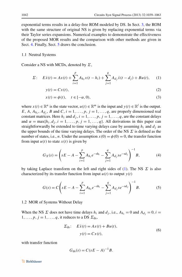
exponential terms results in a delay-free ROM modeled by DS. In Sect. 3, the ROMwith the same structure of original NS is given by replacing exponential terms viatheir Taylor series expansions. Numerical examples to demonstrate the effectivenessof the proposed MOR results and the comparison with other methods are given inSect. 4. Finally, Sect. 5 draws the conclusion.
1.1 Neutral Systems
Consider a NS with MCDs, denoted by Σ ,
Σ : Ex(t) = Ax(t) +p∑
i=1
Ahix(t − hi) +
q∑
j=1
Adjx(t − dj ) + Bu(t), (1)
y(t) = Cx(t), (2)
x(t) = φ(t), t ∈ [−α,0), (3)
where x(t) ∈ Rn is the state vector, u(t) ∈ R
m is the input and y(t) ∈ Rl is the output.
E, A, Ahi, Adj
, B and C, i = 1, . . . , p, j = 1, . . . , q , are properly dimensioned realconstant matrices. Here hi and dj , i = 1, . . . , p, j = 1, . . . , q , are the constant delaysand α = max{hi, dj , i = 1, . . . , p, j = 1, . . . , q}. All derivations in this paper canstraightforwardly be extended to time varying delays case by assuming hi and dj asthe upper bounds of the time varying delays. The order of the NS Σ is defined as thenumber of states, i.e., n. Under the assumption x(0) = φ(0) = 0, the transfer functionfrom input u(t) to state x(t) is given by
GX(s) =(
sE − A −p∑
i=1
Ahie−shi −
q∑
j=1
Adjse−sdj
)−1
B, (4)
by taking Laplace transform on the left and right sides of (1). The NS Σ is alsocharacterized by its transfer function from input u(t) to output y(t)
G(s) = C
(sE − A −
p∑
i=1
Ahie−shi −
q∑
j=1
Adjse−sdj
)−1
B. (5)
1.2 MOR of Systems Without Delay
When the NS Σ does not have time delays hi and dj , i.e., Ahi= 0 and Adj
= 0, i =1, . . . , p, j = 1, . . . , q , it reduces to a DS Σds,
Σds : Ex(t) = Ax(t) + Bu(t),
y(t) = Cx(t),(6)
with transfer function
Gds(s) = C(sE − A)−1B.
Circuits Syst Signal Process (2013) 32:1039–1063 1043
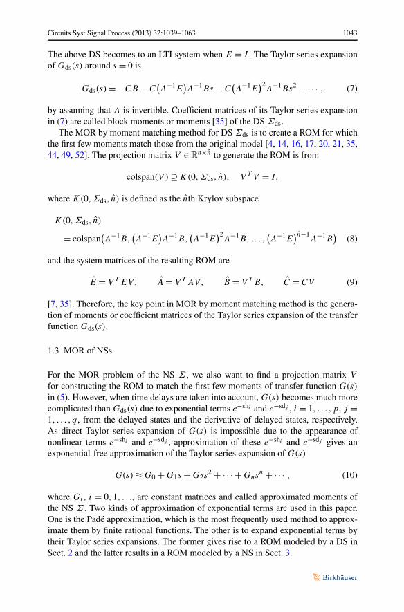
The above DS becomes to an LTI system when E = I . The Taylor series expansionof Gds(s) around s = 0 is
Gds(s) = −CB − C(A−1E
)A−1Bs − C
(A−1E
)2A−1Bs2 − · · · , (7)
by assuming that A is invertible. Coefficient matrices of its Taylor series expansionin (7) are called block moments or moments [35] of the DS Σds.
The MOR by moment matching method for DS Σds is to create a ROM for whichthe first few moments match those from the original model [4, 14, 16, 17, 20, 21, 35,44, 49, 52]. The projection matrix V ∈ R
n×n to generate the ROM is from
colspan(V ) ⊇ K(0,Σds, n), V T V = I,
where K(0,Σds, n) is defined as the nth Krylov subspace
K(0,Σds, n)
= colspan(A−1B,
(A−1E
)A−1B,
(A−1E
)2A−1B, . . . ,
(A−1E
)n−1A−1B
)(8)
and the system matrices of the resulting ROM are
E = V T EV, A = V T AV, B = V T B, C = CV (9)
[7, 35]. Therefore, the key point in MOR by moment matching method is the genera-tion of moments or coefficient matrices of the Taylor series expansion of the transferfunction Gds(s).
1.3 MOR of NSs
For the MOR problem of the NS Σ , we also want to find a projection matrix V
for constructing the ROM to match the first few moments of transfer function G(s)
in (5). However, when time delays are taken into account, G(s) becomes much morecomplicated than Gds(s) due to exponential terms e−shi and e−sdj , i = 1, . . . , p, j =1, . . . , q , from the delayed states and the derivative of delayed states, respectively.As direct Taylor series expansion of G(s) is impossible due to the appearance ofnonlinear terms e−shi and e−sdj , approximation of these e−shi and e−sdj gives anexponential-free approximation of the Taylor series expansion of G(s)
G(s) ≈ G0 + G1s + G2s2 + · · · + Gns
n + · · · , (10)
where Gi , i = 0,1, . . ., are constant matrices and called approximated moments ofthe NS Σ . Two kinds of approximation of exponential terms are used in this paper.One is the Padé approximation, which is the most frequently used method to approx-imate them by finite rational functions. The other is to expand exponential terms bytheir Taylor series expansions. The former gives rise to a ROM modeled by a DS inSect. 2 and the latter results in a ROM modeled by a NS in Sect. 3.
1044 Circuits Syst Signal Process (2013) 32:1039–1063
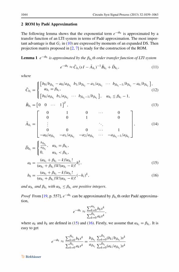
2 ROM by Padé Approximation
The following lemma shows that the exponential term e−shi is approximated by atransfer function of an LTI system in terms of Padé approximation. The most impor-tant advantage is that Gi in (10) are expressed by moments of an expanded DS. Thenprojection matrix proposed in [2, 7] is ready for the construction of the ROM.
Lemma 1 e−shi is approximated by the βhith order transfer function of LTI system
e−shi ≈ Chi(sI − Ahi
)−1Bhi+ Dhi
, (11)
where
Chi=
⎧⎪⎨
⎪⎩
[b0/bβhi
− a0/aβhib1/bβhi
− a1/aβhi· · · bβhi
−1/bβhi− ak/bβhi
],
αhi= βhi
,[b0/aβhi
b1/aβhi· · · bβhi
−1/bβhi
], αhi
≤ βhi− 1,
(12)
Bhi= [
0 0 · · · 1]T
, (13)
Ahi=
⎡
⎢⎢⎢⎢⎢⎣
0 1 0 · · · 00 0 1 0...
. . .
0 0 0 · · · 1−a0/aβhi
−a1/aβhi−a2/aβhi
· · · −aβhi−1/aβhi
⎤
⎥⎥⎥⎥⎥⎦, (14)
Dhi=
⎧⎨
⎩
bβhi
aβhi
, αhi= βhi
,
0, αhi< βhi
,
ak = (αhi+ βhi
− k)!αhi!
(αhi+ βhi
)!k!(αhi− k)!h
ki , (15)
bk = (αhi+ βhi
− k)!αhi!
(αhi+ βhi
)!k!(αhi− k)! (−hi)
k, (16)
and αhiand βhi
with αhi≤ βhi
are positive integers.
Proof From [19, p. 557], e−shi can be approximated by βhith order Padé approxima-
tion,
e−shi ≈∑αhi
k=0 bksk
∑βhi
k=0 aksk,
where ak and bk are defined in (15) and (16). Firstly, we assume that αhi= βhi
. It iseasy to get
e−shi ≈∑βhi
k=0 bksk
∑βhi
k=0 aksk= bβhi
aβhi
∑βhi
k=0(bk/bβhi)sk
∑βhi
k=0(ak/aβhi)sk
Circuits Syst Signal Process (2013) 32:1039–1063 1045
= bβhi
aβhi
+∑βhi
−1k=0 (bk/bβhi
− ak/aβhi)sk
∑βhi
k=0(ak/aβhi)sk
. (17)
It follows by [1, Theorem 3.5.1] that the controllable canonical realization of thesecond term in (17) is equivalent to
Chi(sI − Ahi
)−1Bhi,
which gives (11), with Chi, Ahi
and Bhigiven in (12)–(14). In the case of αhi
=βhi
− 1, i.e., bβhi= 0, (17) becomes a βhi
th order transfer function
e−shi ≈∑βhi
−1k=0 bks
k
∑βhi
k=0 aksk=
∑βhi−1
k=0 (bk/aβhi)sk
sβhi + ∑βhi−1
k=0 (ak/aβhi)sk
, (18)
which results in (11) for the case αhi= βhi
− 1 by the controllable canonical realiza-tion again. The case αhi
< βhi− 1 can be obtained similar to the case αhi
= βhi− 1
by assuming bαhi+1 = · · · = bβhi
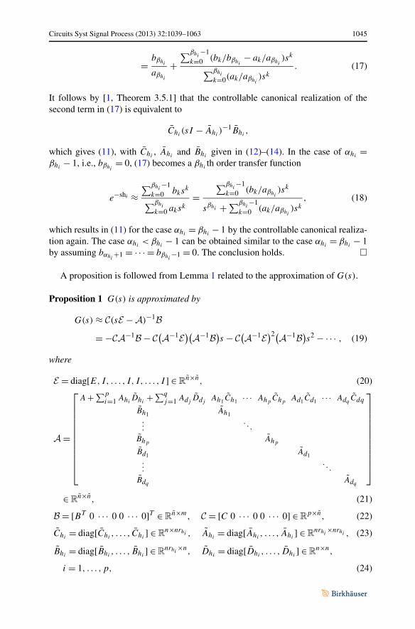
−1 = 0. The conclusion holds. �
A proposition is followed from Lemma 1 related to the approximation of G(s).
Proposition 1 G(s) is approximated by
G(s) ≈ C(sE − A)−1 B
= −C A−1 B − C(
A−1 E)(
A−1 B)s − C
(A−1 E
)2(A−1 B)s2 − · · · , (19)
where
E = diag[E,I, . . . , I, I, . . . , I ] ∈ Rn×n, (20)
A =
⎡
⎢⎢⎢⎢⎢⎢⎢⎢⎢⎢⎢⎢⎣
A + ∑pi=1 Ahi
Dhi+ ∑q
j=1 AdjDdj
Ah1 Ch1 · · · AhpChp
Ad1 Cd1 · · · AdqCdq
Bh1 Ah1...
. . .
BhpAhp
Bd1 Ad1...
. . .
BdqAdq
⎤
⎥⎥⎥⎥⎥⎥⎥⎥⎥⎥⎥⎥⎦
∈ Rn×n, (21)
B = [BT 0 · · · 0 0 · · · 0]T ∈ Rn×m, C = [C 0 · · · 0 0 · · · 0] ∈ R
p×n, (22)
Chi= diag[Chi
, . . . , Chi] ∈ R
n×nrhi , Ahi= diag[Ahi
, . . . , Ahi] ∈ R
nrhi×nrhi , (23)
Bhi= diag[Bhi
, . . . , Bhi] ∈ R
nrhi×n, Dhi
= diag[Dhi, . . . , Dhi
] ∈ Rn×n,
i = 1, . . . , p, (24)
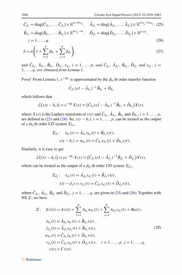
1046 Circuits Syst Signal Process (2013) 32:1039–1063
Cdj= diag[Cdj
, . . . , Cdj] ∈ R
n×nrdj , Adj= diag[Adj
, . . . , Adj] ∈ R
nrdj×nrdj , (25)
Bdj= diag[Bdj
, . . . , Bdj] ∈ R
nrdj×n
, Ddj= diag[Ddj
, . . . , Ddj] ∈ R
n×n,
j = 1, . . . , q, (26)
n = n
(1 +
p∑
i=1
βhi+
q∑
j=1
βdj
), (27)
and Chi, Ahi
, Bhi, Dhi
, rhi, i = 1, . . . , p, and Cdj
, Adj, Bdj
, Ddjand rdj
, j =1, . . . , q , are obtained from Lemma 1.
Proof From Lemma 1, e−shi is approximated by the βhith order transfer function
Chi(sI − Ahi
)−1Bhi+ Dhi
which follows that
L(x(t − hi)
) = e−shi X(s) ≈ (Chi
(sI − Ahi)−1Bhi
+ Dhi
)X(s),
where X(s) is the Laplace transform of x(t) and Chi, Ahi
, Bhiand Dhi
, i = 1, . . . , p,are defined in (23) and (24). So, x(t − hi), i = 1, . . . , p, can be treated as the outputof a βhi
th order LTI system Σhi,
Σhi: xhi
(t) = Ahixhi
(t) + Bhix(t),
x(t − hi) = whi(t) = Chi
xhi(t) + Dhi
x(t).
Similarly, it is easy to get
L(x(t − dj )
) = se−sdj X(s) ≈ (Cdj
(sI − Adj)−1Bdj
+ Ddj
)X(s),
which can be treated as the output of a βdjth order LTI system Σdj
,
Σdj: xdj
(t) = Adjxdj
(t) + Bdjx(t),
x(t − dj ) = rdj(t) = Cdj
xdj(t) + Ddj
x(t),
where Cdj, Adj
, Bdjand Ddj
, j = 1, . . . , q , are given in (25) and (26). Together withNS Σ , we have
Σ : Ex(t) = Ax(t) +p∑
i=1
Ahiwhi
(t) +q∑
j=1
Adjrdj
(t) + Bu(t),
xhi(t) = Ahi
xhi(t) + Bhi
x(t),
xdj(t) = Adj
xdj(t) + Bdj
x(t),
whi(t) = Chi
xhi(t) + Dhi
x(t),
rdj(t) = Cdj
xdj(t) + Ddj
x(t), i = 1, . . . , p, j = 1, . . . , q,
y(t) = Cx(t).
(28)
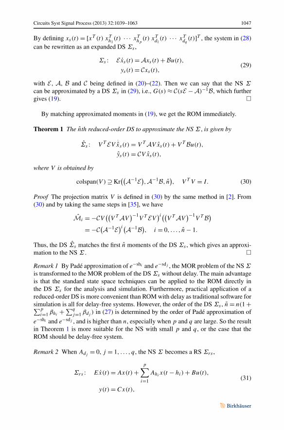
Circuits Syst Signal Process (2013) 32:1039–1063 1047
By defining xs(t) = [xT (t) xTh1
(t) · · · xThp
(t) xTd1
(t) · · · xTdq
(t)]T , the system in (28)can be rewritten as an expanded DS Σs ,
Σs : E xs(t) = Axs(t) + Bu(t),
ys(t) = Cxs(t),(29)
with E , A, B and C being defined in (20)–(22). Then we can say that the NS Σ
can be approximated by a DS Σs in (29), i.e., G(s) ≈ C(sE − A)−1 B, which furthergives (19). �
By matching approximated moments in (19), we get the ROM immediately.
Theorem 1 The nth reduced-order DS to approximate the NS Σ , is given by
Σs : V T E V.
xs(t) = V T AV xs(t) + V T Bu(t),
ys(t) = CV xs(t),
where V is obtained by
colspan(V ) ⊇ Kr((
A−1 E), A−1 B, n
), V T V = I. (30)
Proof The projection matrix V is defined in (30) by the same method in [2]. From(30) and by taking the same steps in [35], we have
Mi = −CV((
V T AV)−1
V T E V)i((
V T AV)−1
V T B)
= −C(
A−1 E)i(A−1 B
), i = 0, . . . , n − 1.
Thus, the DS Σs matches the first n moments of the DS Σs , which gives an approxi-mation to the NS Σ . �
Remark 1 By Padé approximation of e−shi and e−sdj , the MOR problem of the NS Σ
is transformed to the MOR problem of the DS Σs without delay. The main advantageis that the standard state space techniques can be applied to the ROM directly inthe DS Σs for the analysis and simulation. Furthermore, practical application of areduced-order DS is more convenient than ROM with delay as traditional software forsimulation is all for delay-free systems. However, the order of the DS Σs , n = n(1 +∑p
i=1 βhi+ ∑q
j=1 βdj) in (27) is determined by the order of Padé approximation of
e−shi and e−sdj , and is higher than n, especially when p and q are large. So the resultin Theorem 1 is more suitable for the NS with small p and q , or the case that theROM should be delay-free system.
Remark 2 When Adj= 0, j = 1, . . . , q , the NS Σ becomes a RS Σrs ,
Σrs : Ex(t) = Ax(t) +p∑
i=1
Ahix(t − hi) + Bu(t),
y(t) = Cx(t),
(31)
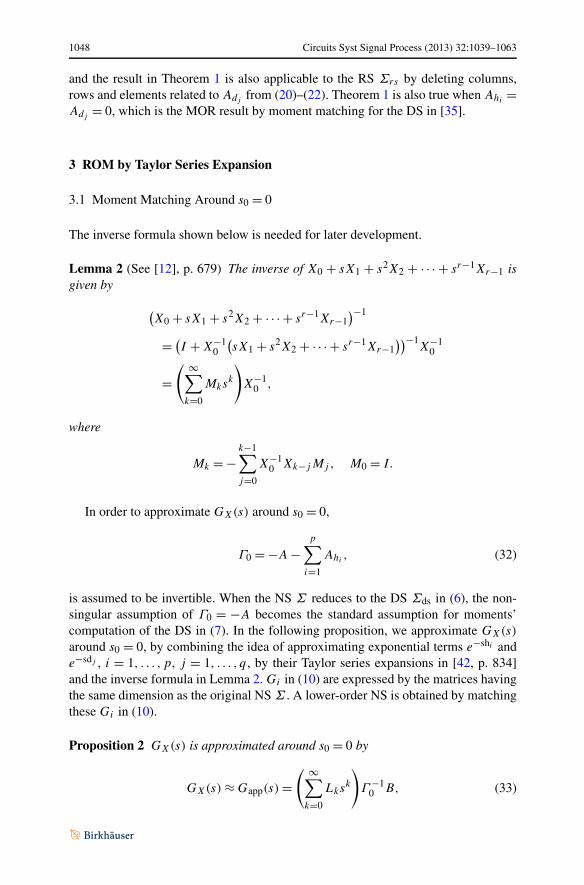
1048 Circuits Syst Signal Process (2013) 32:1039–1063
and the result in Theorem 1 is also applicable to the RS Σrs by deleting columns,rows and elements related to Adj
from (20)–(22). Theorem 1 is also true when Ahi=
Adj= 0, which is the MOR result by moment matching for the DS in [35].
3 ROM by Taylor Series Expansion
3.1 Moment Matching Around s0 = 0
The inverse formula shown below is needed for later development.
Lemma 2 (See [12], p. 679) The inverse of X0 + sX1 + s2X2 + · · · + sr−1Xr−1 isgiven by
(X0 + sX1 + s2X2 + · · · + sr−1Xr−1
)−1
= (I + X−1
0
(sX1 + s2X2 + · · · + sr−1Xr−1
))−1X−1
0
=( ∞∑
k=0
Mksk
)X−1
0 ,
where
Mk = −k−1∑
j=0
X−10 Xk−jMj , M0 = I.
In order to approximate GX(s) around s0 = 0,
Γ0 = −A −p∑
i=1
Ahi, (32)
is assumed to be invertible. When the NS Σ reduces to the DS Σds in (6), the non-singular assumption of Γ0 = −A becomes the standard assumption for moments’computation of the DS in (7). In the following proposition, we approximate GX(s)
around s0 = 0, by combining the idea of approximating exponential terms e−shi ande−sdj , i = 1, . . . , p, j = 1, . . . , q , by their Taylor series expansions in [42, p. 834]and the inverse formula in Lemma 2. Gi in (10) are expressed by the matrices havingthe same dimension as the original NS Σ . A lower-order NS is obtained by matchingthese Gi in (10).
Proposition 2 GX(s) is approximated around s0 = 0 by
GX(s) ≈ Gapp(s) =( ∞∑
k=0
Lksk
)Γ −1
0 B, (33)
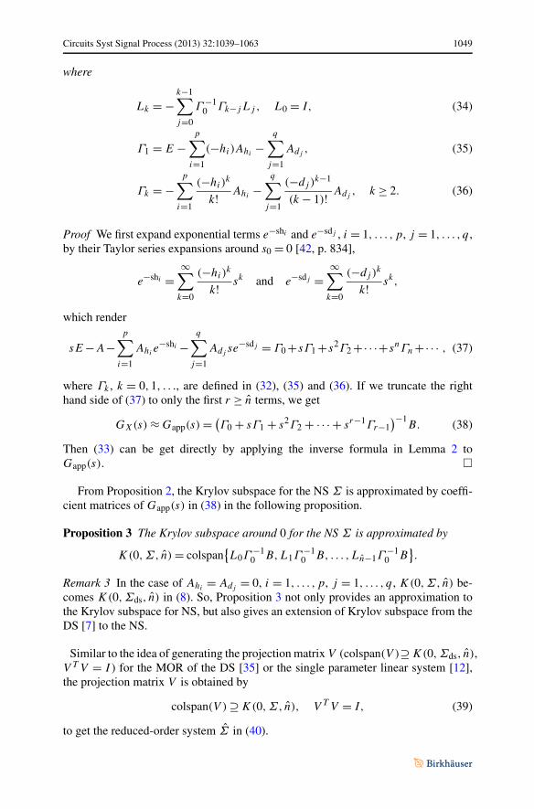
Circuits Syst Signal Process (2013) 32:1039–1063 1049
where
Lk = −k−1∑
j=0
Γ −10 Γk−jLj , L0 = I, (34)
Γ1 = E −p∑
i=1
(−hi)Ahi−
q∑
j=1
Adj, (35)
Γk = −p∑
i=1
(−hi)k
k! Ahi−
q∑
j=1
(−dj )k−1
(k − 1)! Adj, k ≥ 2. (36)
Proof We first expand exponential terms e−shi and e−sdj , i = 1, . . . , p, j = 1, . . . , q ,by their Taylor series expansions around s0 = 0 [42, p. 834],
e−shi =∞∑
k=0
(−hi)k
k! sk and e−sdj =∞∑
k=0
(−dj )k
k! sk,
which render
sE−A−p∑
i=1
Ahie−shi −
q∑
j=1
Adjse−sdj = Γ0 +sΓ1 +s2Γ2 +· · ·+snΓn +· · · , (37)
where Γk , k = 0,1, . . ., are defined in (32), (35) and (36). If we truncate the righthand side of (37) to only the first r ≥ n terms, we get
GX(s) ≈ Gapp(s) = (Γ0 + sΓ1 + s2Γ2 + · · · + sr−1Γr−1
)−1B. (38)
Then (33) can be get directly by applying the inverse formula in Lemma 2 toGapp(s). �
From Proposition 2, the Krylov subspace for the NS Σ is approximated by coeffi-cient matrices of Gapp(s) in (38) in the following proposition.
Proposition 3 The Krylov subspace around 0 for the NS Σ is approximated by
K(0,Σ, n) = colspan{L0Γ
−10 B,L1Γ
−10 B, . . . ,Ln−1Γ
−10 B
}.
Remark 3 In the case of Ahi= Adj
= 0, i = 1, . . . , p, j = 1, . . . , q , K(0,Σ, n) be-comes K(0,Σds, n) in (8). So, Proposition 3 not only provides an approximation tothe Krylov subspace for NS, but also gives an extension of Krylov subspace from theDS [7] to the NS.
Similar to the idea of generating the projection matrix V (colspan(V )⊇ K(0,Σds, n),V T V = I ) for the MOR of the DS [35] or the single parameter linear system [12],the projection matrix V is obtained by
colspan(V ) ⊇ K(0,Σ, n), V T V = I, (39)
to get the reduced-order system Σ in (40).
1050 Circuits Syst Signal Process (2013) 32:1039–1063
Theorem 2 The nth reduced-order NS is given by
Σ :.
x(t) = V T AV x(t) +p∑
i=1
V T AhiV x(t − hi)
+q∑
j=1
V T AdjV
.
x(t − dj ) + V T Bu(t),
y(t) = CV x(t).
(40)
Proof From Proposition 2, X(s) can be approximated by
X(s) = GX(s)U(s)
≈ (Γ0 + sΓ1 + s2Γ2 + · · · + sr−1Γr−1
)−1BU(s)
=( ∞∑
k=0
Lksk
)Γ −1
0 BU(s) = θ(s),
where U(s) is the Laplace transform of u(t). Inspiring from [12, 35], we want tofind a projection matrix V in (39) by matching the first n terms of the approximatedGX(s), which are also first n coefficients of θ(s). By assuming θ(s) = V θ(s), andconsidering
(Γ0 + sΓ1 + s2Γ2 + · · · + sr−1Γr−1
)θ(s) = BU(s)
we obtain
V T(Γ0 + sΓ1 + s2Γ2 + · · · + sn−1Γn−1
)V θ(s) = V T BU(s),
Y (s) ≈ CV θ(s),
where Y(s) is the Laplace transform of y(t). From the expression of Γk , k =0,1, . . . , n − 1, in (32), (35) and (36), it is easy to show that
V T(Γ0 + sΓ1 + s2Γ2 + · · · + sn−1Γn−1
)V θ(s)
= V T
(−A −
p∑
i=1
Ahi
)V + sV T
(E −
p∑
i=1
(−hi)Ahi−
q∑
j=1
Adj
)V
+ · · · + sn−1V T
(−
p∑
i=1
(−hi)n−1
(n − 1)! Ahi−
q∑
j=1
(−dj )n−2
(n − 2)! Adj
)V
= sV T EV − V T AV −p∑
i=1
V T AhiV − s
p∑
i=1
V T (−hi)AhiV
− · · · − sn−1p∑
i=1
(−hi)n−1
(n − 1)! V T AhiV
Circuits Syst Signal Process (2013) 32:1039–1063 1051
− s
(q∑
j=1
V T AdjV − s
q∑
j=1
(−dj )VT Adj
V
− · · · − sn−2q∑
j=1
(−dj )n−2
(n − 2)! V T AdjV
)
≈ sV T EV − V T AV −p∑
i=1
V T AhiV e−shi − s
q∑
j=1
V T AdjV e−sdj .
Consequently, it follows that
V T(Γ0 + sΓ1 + s2Γ2 + · · · + sn−1Γn−1
)V θ(s)
≈(
sV T EV − V T AV −p∑
i=1
V T AhiV e−shi − s
q∑
j=1
V T AdjV e−sdj
)θ (s)
= V T BU(s)
which is equivalent to the reduced-order NS Σ , where x(t) is the inverse Laplacetransform of θ (s). �
Corollary 1 The result in Theorem 2 is still true for the RS Σrs in (31) by takingAdj
= 0, j = 1, . . . , q , from (35) and (36). In the case of p = q = 1, the projectionmatrix V in (39) is given by
colspan(V ) ⊇ K(0,Σ, n), V T V = I,
Lk = −k−1∑
j=0
Γ −10 Γk−jLj , L0 = I,
Γ0 = −A − Ah1, Γ1 = E + h1Ah1 − Ad1 ,
Γk = − (−h1)k
k! Ah1 − (−d1)k−1
(k − 1)! Ad1 , k ≥ 2.
Remark 4 The MOR result in [42] considers the reduction of a special kind of RSwith C = BT . The moments of this special RS are approximated by the moments ofa large scale DS with system matrices given by
C =
⎡
⎢⎢⎢⎣
Γ1 Γ2 · · · Γr
In
. . .
In 0
⎤
⎥⎥⎥⎦ ∈ Rrn×rn, G =
⎡
⎢⎢⎢⎣
Γ0−In
. . .
−In
⎤
⎥⎥⎥⎦ ∈ Rrn×rn,
L = [BT 0 · · · 0
]T ∈ Rrn×m,
where r is defined in (38). This will result in two obvious shortcomings. One is thatthe dimension of ROM may be higher than the original RS as low-order ROM may
1052 Circuits Syst Signal Process (2013) 32:1039–1063
cause large error. The other is that high-order system matrices C , G and L make thismethod fail to reduce higher-order RS as the storage of C , G and L can be memory-demanding. Fortunately, Proposition 2 avoids this by using the inverse formula inLemma 2 to produce moments having the same dimension as the original NS. Thecomparison with the result in [42, p. 834] is shown in Examples 2 and 3 in Sect. 4.
Remark 5 The MOR problems with ROM in NS form are also investigated in [43]and [45], respectively, by guaranteeing that the H∞ norm or energy-to-peak gain ofthe error system is less than a given scalar in terms of LMIs with inverse constraints.It is solved by CCL algorithm [13] by transforming it to a minimization problemsubject to original LMIs and additional LMIs coming from the inverse constraints,which are further solved by IPM. However, IPM requires that all matrix variablesare transformed to a very huge vector variable in [8]. Obviously, this may render anout of memory problem due to large size matrix variables, and this further results inIPM not being able to handle large scale LMIs. Moreover, the computational cost ofsolving LMIs with inverse constraints is very high because of solving a minimizationproblem. Although LMI-based method provides a good approximation of the originalNS by ensuring global accuracy, as a trade-off, high computational cost makes itinapplicable to reduce high-order NS with MCDs. The comparison with the methodsin [43] and [45] is given in Example 4 in Sect. 4.
3.2 Extension to the Point s0 �= 0 and multi-point moment matching
The result in Theorem 2 is extended to a nonzero point s0 in the following theorem.Assume that
Υ0(s0) = s0E − A −p∑
i=1
e−s0hi Ahi−
q∑
j=1
s0e−s0dj Adj
, (41)
is nonsingular in order to approximate GX(s) around s0.
Theorem 3 The projection matrix V is obtained from the approximated Krylov sub-space around s0
colspan(V ) ⊇ K(s0,Σ, n), V T V = I, (42)
the nth reduced-order NS is given by
Σ :.
x(t) = V T AV x(t) +p∑
i=1
V T AhiV x(t − hi)
+q∑
j=1
V T AdjV
.
x(t − dj ) + V T Bu(t),
y(t) = CV x(t),
Circuits Syst Signal Process (2013) 32:1039–1063 1053
where
K(s0,Σ, n) = colspan{J0(s0)Υ
−10 (s0)B,J1(s0)Υ
−10 (s0)B, . . . , Jn−1(s0)Υ
−10 (s0)B
},
(43)
Jk(s0) = −k−1∑
j=0
Υ −10 (s0)Υk−j (s0)Jj (s0), J0(s0) = I, (44)
Υ1(s0) = E −p∑
i=1
(−hi)e−s0hi Ahi
−q∑
j=1
(s0(−dj ) + 1
)e−s0dj Adj
, (45)
Υk(s0) = −p∑
i=1
(−hi)k
k! e−s0hi Ahi−
q∑
j=1
(s0
(−dj )k
k! + (−dj )k−1
(k − 1)!)
e−s0dj Adj,
k ≥ 2. (46)
Proof By expanding e−shi and e−sdj , i = 1, . . . , p, j = 1, . . . , q , by their Taylor se-ries expansions around s0,
e−shi =∞∑
k=0
e−s0hi(−hi)
k
k! (s − s0)k and e−sdj =
∞∑
k=0
e−s0dj(−dj )
k
k! (s − s0)k,
we have
sE − A −p∑
i=1
Ahie−shi −
q∑
j=1
Adjse−sdj
= sE − A −p∑
i=1
Ahie−shi −
q∑
j=1
s0Adje−sdj −
q∑
j=1
(s − s0)Adje−sdj
= (s − s0)E + s0E − A −p∑
i=1
Ahi
∞∑
k=0
e−s0hi(−hi)
k
k! (s − s0)k
−q∑
j=1
s0Adj
∞∑
k=0
e−s0dj(−dj )
k
k! (s − s0)k
−q∑
j=1
Adj
∞∑
k=0
e−s0dj(−dj )
k
k! (s − s0)k+1
= s0E − A −p∑
i=1
e−s0hi Ahi−
q∑
j=1
s0e−s0dj Adj
+ (s − s0)
(E −
p∑
i=1
(−hi)e−s0hi Ahi
−q∑
j=1
(s0(−dj ) + 1
)e−s0dj Adj
)
1054 Circuits Syst Signal Process (2013) 32:1039–1063
+ (s − s0)2
(−
p∑
i=1
(−hi)2
2! e−s0hi Ahi−
q∑
j=1
(s0
(−dj )2
2! + (−dj )
1!)
e−s0dj Adj
)
+ · · · + (s − s0)n
(−
p∑
i=1
(−hi)n
n! e−s0hi Ahi
−q∑
j=1
(s0
(−dj )n
n! + (−dj )n−1
(n − 1)!)
e−s0dj Adj
)+ · · ·
= Υ0(s0) + (s − s0)Υ1(s0) + (s − s0)2Υ2(s0) + · · · + (s − s0)
nΥn(s0) + · · · ,
where Υk , k = 0,1, . . ., are defined in (41), (45) and (46). Then the proof can befinished similarly to the proof in Proposition 2 and Theorem 2. �
Theorem 3 can be further extended to the multi-point case.
Corollary 2 The projection matrix V in (42) obtained from the approximated Krylovsubspace around multiple points, s1, s2, . . . , sg is given by
colspan(V ) ⊇g⋃
i=1
K(si,Σ, n), V T V = I,
where K(si,Σ, n), i = 1, . . . , g, are defined in (43).
4 Numerical Examples
All the computation described in this section is performed in Intel Core 2 Quad pro-cessors with CPU 2.66 GHz and 2.87 GB memory. The first example is to show thatwith the same order of the ROM, Taylor series expansion method is better than Padéapproximation method although it provides a delay-free ROM with better simulationand analysis than systems with delay via the standard state space techniques.
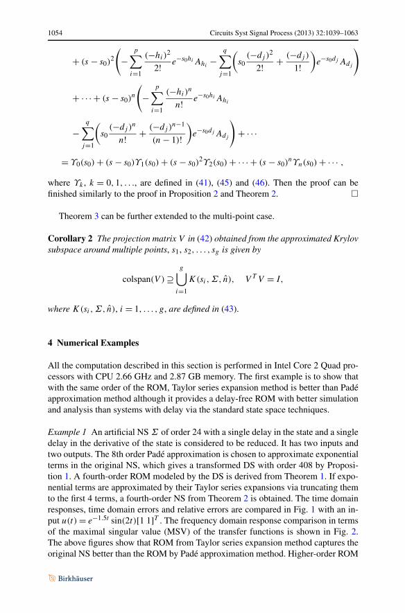
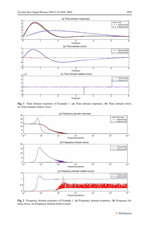
Example 1 An artificial NS Σ of order 24 with a single delay in the state and a singledelay in the derivative of the state is considered to be reduced. It has two inputs andtwo outputs. The 8th order Padé approximation is chosen to approximate exponentialterms in the original NS, which gives a transformed DS with order 408 by Proposi-tion 1. A fourth-order ROM modeled by the DS is derived from Theorem 1. If expo-nential terms are approximated by their Taylor series expansions via truncating themto the first 4 terms, a fourth-order NS from Theorem 2 is obtained. The time domainresponses, time domain errors and relative errors are compared in Fig. 1 with an in-put u(t) = e−1.5t sin(2t)[1 1]T . The frequency domain response comparison in termsof the maximal singular value (MSV) of the transfer functions is shown in Fig. 2.The above figures show that ROM from Taylor series expansion method captures theoriginal NS better than the ROM by Padé approximation method. Higher-order ROM
Circuits Syst Signal Process (2013) 32:1039–1063 1055
Fig. 1 Time domain responses of Example 1. (a) Time domain responses. (b) Time domain errors.(c) Time domain relative errors
Fig. 2 Frequency domain responses of Example 1. (a) Frequency domain responses. (b) Frequency do-main errors. (c) Frequency domain relative errors
1056 Circuits Syst Signal Process (2013) 32:1039–1063
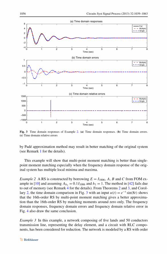
Fig. 3 Time domain responses of Example 2. (a) Time domain responses. (b) Time domain errors.(c) Time domain relative errors
by Padé approximation method may result in better matching of the original system(see Remark 1 for the details).
This example will show that multi-point moment matching is better than single-point moment matching especially when the frequency domain response of the orig-inal system has multiple local minima and maxima.
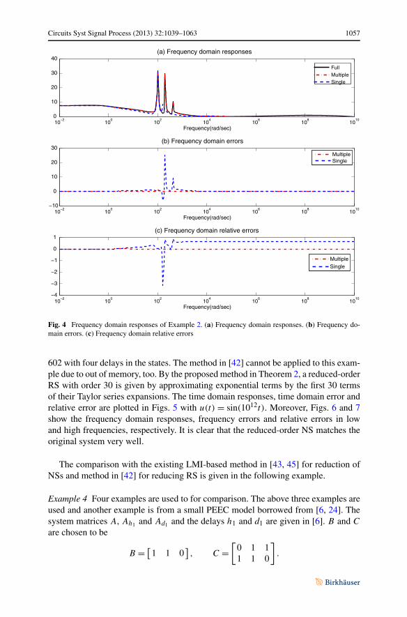
Example 2 A RS is constructed by borrowing E = I1006, A, B and C from FOM ex-ample in [10] and assuming Ah1 = 0.1I1006 and h1 = 1. The method in [42] fails dueto out of memory (see Remark 4 for the details). From Theorems 2 and 3, and Corol-lary 2, the time domain comparison in Fig. 3 with an input u(t) = e−t sin(8t) showsthat the 16th-order RS by multi-point moment matching gives a better approxima-tion than the 16th-order RS by matching moments around zero only. The frequencydomain responses, frequency domain errors and frequency domain relative error inFig. 4 also draw the same conclusion.
Example 3 In this example, a network composing of five lands and 50 conductorstransmission line, representing the delay element, and a circuit with RLC compo-nents, has been considered for reduction. The network is modeled by a RS with order
Circuits Syst Signal Process (2013) 32:1039–1063 1057
Fig. 4 Frequency domain responses of Example 2. (a) Frequency domain responses. (b) Frequency do-main errors. (c) Frequency domain relative errors
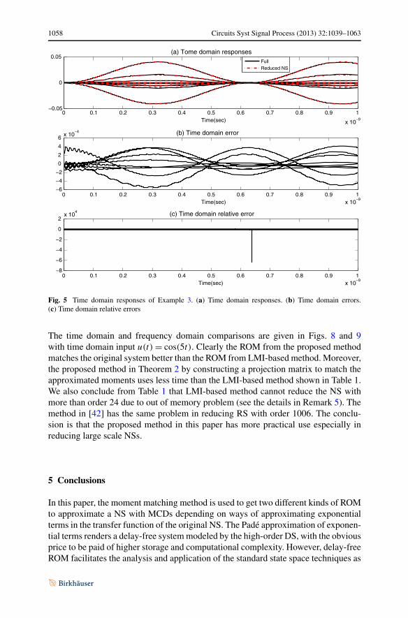
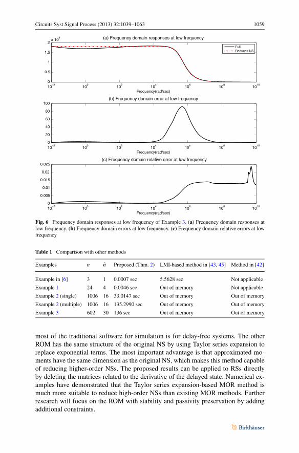
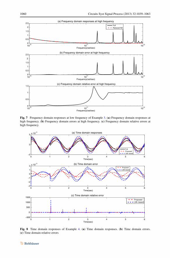
602 with four delays in the states. The method in [42] cannot be applied to this exam-ple due to out of memory, too. By the proposed method in Theorem 2, a reduced-orderRS with order 30 is given by approximating exponential terms by the first 30 termsof their Taylor series expansions. The time domain responses, time domain error andrelative error are plotted in Figs. 5 with u(t) = sin(1012t). Moreover, Figs. 6 and 7show the frequency domain responses, frequency errors and relative errors in lowand high frequencies, respectively. It is clear that the reduced-order NS matches theoriginal system very well.
The comparison with the existing LMI-based method in [43, 45] for reduction ofNSs and method in [42] for reducing RS is given in the following example.
Example 4 Four examples are used to for comparison. The above three examples areused and another example is from a small PEEC model borrowed from [6, 24]. Thesystem matrices A, Ah1 and Ad1 and the delays h1 and d1 are given in [6]. B and C
are chosen to be
B = [1 1 0
], C =
[0 1 11 1 0
].
1058 Circuits Syst Signal Process (2013) 32:1039–1063
Fig. 5 Time domain responses of Example 3. (a) Time domain responses. (b) Time domain errors.(c) Time domain relative errors
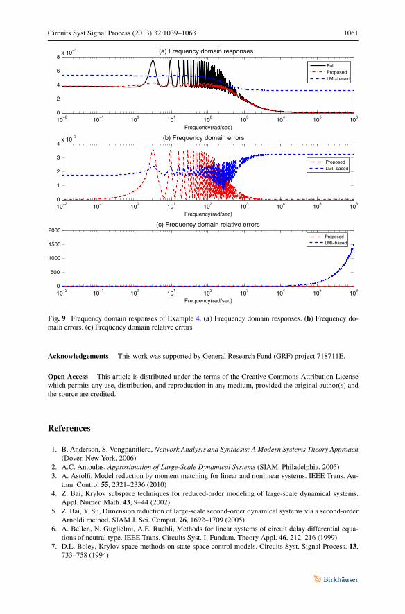
The time domain and frequency domain comparisons are given in Figs. 8 and 9with time domain input u(t) = cos(5t). Clearly the ROM from the proposed methodmatches the original system better than the ROM from LMI-based method. Moreover,the proposed method in Theorem 2 by constructing a projection matrix to match theapproximated moments uses less time than the LMI-based method shown in Table 1.We also conclude from Table 1 that LMI-based method cannot reduce the NS withmore than order 24 due to out of memory problem (see the details in Remark 5). Themethod in [42] has the same problem in reducing RS with order 1006. The conclu-sion is that the proposed method in this paper has more practical use especially inreducing large scale NSs.
5 Conclusions
In this paper, the moment matching method is used to get two different kinds of ROMto approximate a NS with MCDs depending on ways of approximating exponentialterms in the transfer function of the original NS. The Padé approximation of exponen-tial terms renders a delay-free system modeled by the high-order DS, with the obviousprice to be paid of higher storage and computational complexity. However, delay-freeROM facilitates the analysis and application of the standard state space techniques as
Circuits Syst Signal Process (2013) 32:1039–1063 1059
Fig. 6 Frequency domain responses at low frequency of Example 3. (a) Frequency domain responses atlow frequency. (b) Frequency domain errors at low frequency. (c) Frequency domain relative errors at lowfrequency
Table 1 Comparison with other methods
Examples n n Proposed (Thm. 2) LMI-based method in [43, 45] Method in [42]
Example in [6] 3 1 0.0007 sec 5.5628 sec Not applicable
Example 1 24 4 0.0046 sec Out of memory Not applicable
Example 2 (single) 1006 16 33.0147 sec Out of memory Out of memory
Example 2 (multiple) 1006 16 135.2990 sec Out of memory Out of memory
Example 3 602 30 136 sec Out of memory Out of memory
most of the traditional software for simulation is for delay-free systems. The otherROM has the same structure of the original NS by using Taylor series expansion toreplace exponential terms. The most important advantage is that approximated mo-ments have the same dimension as the original NS, which makes this method capableof reducing higher-order NSs. The proposed results can be applied to RSs directlyby deleting the matrices related to the derivative of the delayed state. Numerical ex-amples have demonstrated that the Taylor series expansion-based MOR method ismuch more suitable to reduce high-order NSs than existing MOR methods. Furtherresearch will focus on the ROM with stability and passivity preservation by addingadditional constraints.
1060 Circuits Syst Signal Process (2013) 32:1039–1063
Fig. 7 Frequency domain responses at low frequency of Example 3. (a) Frequency domain responses athigh frequency. (b) Frequency domain errors at high frequency. (c) Frequency domain relative errors athigh frequency.
Fig. 8 Time domain responses of Example 4. (a) Time domain responses. (b) Time domain errors.(c) Time domain relative errors
Circuits Syst Signal Process (2013) 32:1039–1063 1061
Fig. 9 Frequency domain responses of Example 4. (a) Frequency domain responses. (b) Frequency do-main errors. (c) Frequency domain relative errors
Acknowledgements This work was supported by General Research Fund (GRF) project 718711E.
Open Access This article is distributed under the terms of the Creative Commons Attribution Licensewhich permits any use, distribution, and reproduction in any medium, provided the original author(s) andthe source are credited.
References
1. B. Anderson, S. Vongpanitlerd, Network Analysis and Synthesis: A Modern Systems Theory Approach(Dover, New York, 2006)
2. A.C. Antoulas, Approximation of Large-Scale Dynamical Systems (SIAM, Philadelphia, 2005)3. A. Astolfi, Model reduction by moment matching for linear and nonlinear systems. IEEE Trans. Au-
tom. Control 55, 2321–2336 (2010)4. Z. Bai, Krylov subspace techniques for reduced-order modeling of large-scale dynamical systems.
Appl. Numer. Math. 43, 9–44 (2002)5. Z. Bai, Y. Su, Dimension reduction of large-scale second-order dynamical systems via a second-order
Arnoldi method. SIAM J. Sci. Comput. 26, 1692–1709 (2005)6. A. Bellen, N. Guglielmi, A.E. Ruehli, Methods for linear systems of circuit delay differential equa-
tions of neutral type. IEEE Trans. Circuits Syst. I, Fundam. Theory Appl. 46, 212–216 (1999)7. D.L. Boley, Krylov space methods on state-space control models. Circuits Syst. Signal Process. 13,
733–758 (1994)
1062 Circuits Syst Signal Process (2013) 32:1039–1063
8. S. Boyd, L. EL Ghaoui, E. Feron, N. Balakrishnan, Linear Matrix Inequalities in System and ControlTheory (SIAM, Philadelphia, 1994)
9. S. Cauet, F. Hutu, P. Coirault, Time-varying delay passivity analysis in 4 GHz antennas array design.Circuits Syst. Signal Process. 31, 93–106 (2012)
10. Y. Chahlaoui, P. Van Dooren, A collection of benchmark examples for model reduction of lin-ear time invariant dynamical systems. Publishing Physics Web. http://www.icm.tu-bs.de/NICONET/benchmodred.html (2010)
11. Q. Chen, N. Wong, Efficient numerical modeling of random rough surface effects in interconnectresistance extraction. Int. J. Circuit Theory Appl. 37, 751–763 (2009)
12. L. Daniel, O.C. Siong, L.S. Chay, K.H. Lee, J. White, A multiparameter moment-matching model-reduction approach for generating geometrically parameterized interconnect performance models.IEEE Trans. Comput.-Aided Des. Integr. Circuits Syst. 23, 678–693 (2004)
13. L. El Ghaoui, F. Oustry, M. AitRami, A cone complementarity linearization algorithm for staticoutput-feedback and related problems. IEEE Trans. Autom. Control 42, 1171–1176 (1997)
14. P. Feldmann, R.W. Freund, Efficient linear circuit analysis by Padé approximation via the Lanczosprocess. IEEE Trans. Comput.-Aided Des. Integr. Circuits Syst. 14, 639–649 (1995)
15. L. Fortuna, G. Nunnari, A. Gallo, Model Order Reduction Techniques, with Applications in ElectricalEngineering (Springer, Berlin, 1992)
16. R.W. Freund, SPRIM: structure-preserving reduced-order interconnect macromodeling, in IEEE/ACMInternational Conference on Computer Aided Design (2004), pp. 80–87
17. K. Gallivan, E. Grimme, P. Van Dooren, A rational Lanczos algorithm for model reduction. Numer.Algorithm 12, 33–63 (1996)
18. H. Gao, T. Chen, J. Lam, A new delay system approach to network-based control. Automatica 44,39–52 (2008)
19. G.H. Golub, C.F. Van Loan, Matrix Computations (Johns Hopkins University Press, Baltimore, 1989)20. E. Grimme, Krylov projection methods for model reduction. PhD thesis, University of Illinois at
Urbana-Champaign (1997)21. E.J. Grimme, D.C. Sorensen, P. Van Dooren, Model reduction of state space systems via an implicitly
restarted Lanczos method. Numer. Algorithm 12, 1–31 (1996)22. T. Hamamoto, T. Song, T. Katayama, T. Shimamoto, Complexity reduction algorithm for hierarchical
B-picture of H.264/SVC. Int. J. Innov. Comput., Inf. Control 7, 445–457 (2011)23. Q.-L. Han, Robust stability of uncertain delay-differential systems of neutral type. Automatica 38,
719–723 (2002)24. Q.-L. Han, Stability analysis for a partial element equivalent circuit (PEEC) model of neutral type.
Int. J. Circuit Theory Appl. 33, 321–332 (2005)25. H.-L. Hung, Y.F. Huang, Peak to average power ratio reduction of multicarrier transmission systems
using electromagnetism-like method. Int. J. Innov. Comput., Inf. Control 7, 2037–2050 (2008)26. S. Lall, J.E. Marsden, S. Glavaški, A subspace approach to balanced truncation for model reduction
of nonlinear control systems. Int. J. Innov. Comput., Inf. Control 12, 519–535 (2002)27. J. Lam, Model reduction of delay systems using Padé approximants. Int. J. Control 57, 377–391
(1993)28. J. Lam, H. Gao, C. Wang, Stability analysis for continuous systems with two additive time-varying
delay components. Syst. Control Lett. 56, 16–24 (2007)29. Y. Li, J. Lam, X. Luo, Convex optimization approaches to robust L1 fixed-order filtering for polytopic
systems with multiple delays. Circuits Syst. Signal Process. 27, 1–22 (2008)30. G.R. Naik, D.K. Kumar, Dimensional reduction using blind source separation for identifying sources.
Int. J. Innov. Comput., Inf. Control 7, 989–1000 (2011)31. N.M. Nakhla, A. Dounavis, R. Achar, M.S. Nakhla, DEPACT: Delay extraction-based passive com-
pact transmission-line macromodeling algorithm. IEEE Trans. Adv. Packag. 28, 13–23 (2005)32. S.-I. Niculescu, On delay-dependent stability under model transformations of some neutral linear
systems. Int. J. Control 74, 609–617 (2001)33. D. Ning, J. Roychowdhury, General-purpose nonlinear model-order reduction using piecewise-
polynomial representations. IEEE Trans. Comput.-Aided Des. Integr. Circuits Syst. 27, 249–264(2008)
34. G. Obinata, B.D.O. Anderson, Model Reduction for Control System Design (Springer, Berlin, 2001)35. A. Odabasioglu, M. Celik, L.T. Pileggi, PRIMA: passive reduced-order interconnect macromodeling
algorithm. IEEE Trans. Comput.-Aided Des. Integr. Circuits Syst. 17, 645–654 (1998)36. J.R. Phillips, Projection-based approaches for model reduction of weakly nonlinear time-varying sys-
tems. IEEE Trans. Comput.-Aided Des. Integr. Circuits Syst. 22, 171–187 (2003)
Circuits Syst Signal Process (2013) 32:1039–1063 1063
37. J. Qiu, H. Yang, P. Shi, Y. Xia, Robust H∞ control for class of discrete-time Markovian jump systemswith time-varying delays based on delta operator. Circuits Syst. Signal Process. 27, 627–643 (2008)
38. J.-P. Richard, Time-delay systems: an overview of some recent advances and open problems. Auto-matica 39, 1667–1694 (2003)
39. B. Song, S. Xu, Y. Zou, Delay-dependent robust H∞ filtering for uncertain neutral stochastic time-delay systems. Circuits Syst. Signal Process. 28, 241–256 (2009)
40. X. Su, L. Wu, P. Shi, Y.-D. Song, H∞ model reduction of Takagi-Sugeno fuzzy stochastic sys-tems. IEEE Trans. Syst., Man, Cybern., B, Cybern. Online version http://ieeexplore.ieee.org/stamp/stamp.jsp?arnumber=06202714
41. T.J. Tsai, J.S.H. Tsai, S.M. Guo, G. Chen, An optimal linear-quadratic digital tracker for analogneutral time-delay systems. IMA J. Math. Control Inf. 23, 43–66 (2006)
42. W.L. Tseng, C.Z. Chen, E. Gad, M. Nakhla, R. Achar, Passive order reduction for RLC circuits withdelay elements. IEEE Trans. Adv. Packag. 30, 830–840 (2007)
43. Q. Wang, J. Lam, S. Xu, Delay-dependent energy-to-peak model reduction neutral systems with time-varying delays, in Proceedings of the 7th Asia-Pacific Conference on Complex Systems (2004), pp.448–461
44. Q. Wang, J. Lam, S. Xu, H. Gao, Delay-dependent and delay-independent energy-to-peak modelapproximation for systems with time-varying delay. Int. J. Syst. Sci. 36, 445–460 (2005)
45. Q. Wang, J. Lam, S. Xu, L. Zhang, Delay-dependent γ -suboptimal H∞ model reduction for neutralsystems with time-varying delays. J. Dyn. Syst. Meas. Control 128, 364–399 (2006)
46. X. Wang, Q. Wang, Z. Zhang, Q. Chen, N. Wong, Balanced truncation for time-delay systems viaapproximate Gramians, in 16th Asia and South Pacific Design Automation Conference (ASP-DAC)(2011), pp. 55–60
47. Z. Wang, J. Lam, K.J. Burnham, Stability analysis and observer design for neutral delay system. IEEETrans. Autom. Control 47, 478–483 (2002)
48. N. Wong, V. Balakrishnan, Fast positive-real balanced truncation via quadratic alternating directionimplicit iteration. IEEE Trans. Comput.-Aided Des. Integr. Circuits Syst. 26, 1725–1731 (2007)
49. L. Wu, P. Shi, H. Gao, C. Wang, A new approach to robust H∞ filtering for uncertain systems withboth discrete and distributed delays. Circuits Syst. Signal Process. 26, 229–247 (2007)
50. L. Wu, P. Shi, H. Gao, J. Wang, H∞ model reduction for linear parameter-varying systems withdistributed delay. Int. J. Control 82, 408–422 (2009)
51. L. Wu, X. Su, P. Shi, J. Qiu, Model approximation for discrete-time state-delay systems in the T-Sfuzzy framework. IEEE Trans. Fuzzy Syst. 19, 366–378 (2011)
52. L. Wu, W.X. Zheng, Weighted H∞ model reduction for linear switched systems with time-varyingdelay. Automatica 45, 186–193 (2009)
53. S. Xu, J. Lam, New positive realness conditions for uncertain discrete descriptor systems: analysisand synthesis. IEEE Trans. Circuits Syst. I, Fundam. Theory Appl. 51, 1897–1905 (2004)
54. S. Xu, J. Lam, S. Huang, C. Yang, H∞ model reduction for linear time-delay systems: continuous-time case. Int. J. Control 74, 1062–1074 (2001)
55. S. Xu, J. Lam, On H∞ filtering for a class of uncertain nonlinear neutral systems. Circuits Syst. SignalProcess. 23, 215–230 (2004)
56. S. Xu, J. Lam, H. Gao, Y. Zou, Robust H∞ filtering for uncertain discrete stochastic systems withtime delays. Circuits Syst. Signal Process. 24, 753–770 (2005)
57. R. Yang, H. Gao, J. Lam, P. Shi, New stability criteria for neural networks with distributed and prob-abilistic delays. Circuits Syst. Signal Process. 28, 505–522 (2009)
58. Z. Zhang, N. Wong, Passivity test of immittance descriptor systems based on generalized Hamiltonianmethods. IEEE Trans. Circuits Syst. II, Analog Digit. Signal Process. 57, 61–65 (2010)
59. W. Zhou, D. Tong, H. Lu, Q. Zhong, J. Fang, Time-delay dependent H∞ model reduction for un-certain stochastic systems: continuous-time case. Circuits Syst. Signal Process. 30, 941–961 (2011)