Embed Size (px)
Citation preview

Title:
A Novel Business Process Prediction Model Using a Deep Learning Method
Authors:
1. Nijat Mehdiyev (M.Sc.)
Institute for Information Systems (IWi)
German Research Center for Artificial Intelligence (DFKI) and Saarland University
Campus D3.2, 66123
Saarbruecken, Germany
2. Joerg Evermann (Prof. Dr.)
Memorial University of Newfoundland
310 Elizabeth Avenue, NL, A1B 3X5
St. John’s, NL, Canada
3. Peter Fettke (Prof. Dr.)
Institute for Information Systems (IWi)
German Research Center for Artificial Intelligence (DFKI) and Saarland University
Campus D3.2, 66123
Saarbruecken, Germany
Title Page

A Novel Business Process Prediction Model Using a Deep Learning Method
Abstract
The ability to proactively monitor business processes is a main competitive differentiator for
firms. Process execution logs generated by Process Aware Information Systems (PAIS) help
to make process specific predictions for enabling a proactive situational awareness. The goal
of the proposed approach is to predict the next process event from the completed activities of
the running process instance, based on the execution log data from previously completed
process instances. By predicting process events, companies can initiate timely interventions to
address undesired deviations from the desired workflow. We propose a multi-stage deep
learning approach that formulates the next event prediction problem as a classification problem.
Following a feature pre-processing stage with n-grams and feature hashing, we apply a deep
learning model consisting of an unsupervised pre-training component with stacked
autoencoders and a supervised fine-tuning component. Experiments on a variety of business
process log datasets show that our multi-stage deep learning approach provides promising
results. We also compared our results to existing deep recurrent neural networks and
conventional classification approaches. Furthermore, we address the identification of suitable
hyperparameters for the proposed approach, and the handling of the imbalanced nature of
business process event datasets.
Keywords: Process prediction; Deep learning; Feature hashing; N-grams; Stacked
autoencoders.
1. Introduction
High-performance business processes are one of the last points of differentiation (Davenport
and Harris 2007). Embedding predictive analytics into enterprise processes can boost business
value (LaValle et al. 2011). Process aware enterprise information systems (EIS) such as
Workflow Management Systems (WMS), Enterprise Resource Planning (ERP), Customer
Relationship Management (CRM), or Incident Management (IM), generate log events during
process execution (van der Aalst et al. 2011). Such logs are a source for predictive analytics,
which aids decision making by providing insights into future process behavior. An effective
design and implementation of predictive approaches ensure that business activities will run in
a desired manner by avoiding predicted failures and deviations from the intended process
behavior. Detecting process anomalies in real-time, analyzing behavioral patterns of customers
to make tailored offers, risk management by predicting compliance violations, or effective
resource allocation, are some of the use cases of data driven predictive process analytics
(Evermann et al. 2017).
Current EIS focus on enhancing a company’s ability to achieve high-performing business
processes. However, their effectiveness is limited by their lack of advanced predictive
analytics. The built-in business intelligence solutions mainly address descriptive, such as
demographic and performance problems. However, simply making operations more efficient
is not enough for firms to remain competitive. They face challenges to transform the vast
amount of generated data into smart decisions to deliver better products and services (Duan
and Da Xu 2012). Hence, future EIS need to shift from diagnostic examination of historical
data to proactive decision making using predictive analytics. Predictive capabilities need to be
embedded into the business processes. As process orchestration tools, EIS provide the
necessary basis for this. Integrating advanced analytics with EIS is an important emerging trend
in IS research (Sun et al. 2015).
Blinded Manuscript Resubmission Click here to view linked References
1 2 3 4 5 6 7 8 9 10 11 12 13 14 15 16 17 18 19 20 21 22 23 24 25 26 27 28 29 30 31 32 33 34 35 36 37 38 39 40 41 42 43 44 45 46 47 48 49 50 51 52 53 54 55 56 57 58 59 60 61 62 63 64 65

Business process prediction predicts a target variable of interest after extracting features from
business process log data. Predicting continuous target values, such as remaining process
execution time, are regression problems. Predicting discrete target values, such as the next
events in the running case, the outcome of a process instance, or the violation of service level
agreements, are classification problems. In this study, we focus on predicting the next business
process event, considering the past events of the running process instance, based on execution
log data from previously completed process instances. This is an important problem in process
analytics as such analytical information allows analysts to intervene proactively to prevent
undesired behavior. We address this problem with a multi-stage deep learning approach. The
main contribution of our research is threefold:
1. This study applies, for the first time in the business process management domain, a
deep learning approach consisting of an unsupervised pre-training stage with stacked
autoencoders, and a supervised fine-tuning stage for the multi-class classification
problem. By initializing the parameters in all neural networks layers using greedy
layerwise pre-training with autoencoders, followed by a minimization of a global
training criterion using labels, we improve on current process prediction methods.
2. This study improves on prior research by incorporating an extensive data pre-
processing stage. We use an n-gram representation and feature hashing approach to
build numerical feature vectors from event log data. To our knowledge, no prior studies
have applied feature hashing in this domain. Encoding process data so as to take into
consideration their sequential nature, and reducing the dimensionality of this encoding
to speed up the inference process of the deep neural networks, are crucial tasks that
were examine carefully in our study.
3. We address the hyperparameter optimization of our deep learning approach, and the
imbalanced nature of the process data to further improve prediction precision.
We follow the “exaptation” (extend known solutions to new problems) type of Design Science
Research (DSR) knowledge contribution by adopting successful solutions (stacked
autoencoders based deep learning, feature hashing) to build innovative predictive analytics
models for process data in EIS (Gregor and Hevner 2013).
The remainder of the paper is organized as follows: Section 2 introduces related work on
business process prediction. Section 3 provides a broad description of the components of the
proposed approach. It discusses the data pre-processing stages, n-gram encoding and feature
hashing, and the structure of the deep learning model. Section 4 outlines the experimental
settings, the structure of datasets and our empirical results. Section 5 concludes the paper with
a discussion and summary.
2. Related Work
A growing body of literature has examined machine-learning approaches in business process
management. We categorize them according to the type of the target variable (discrete vs.
continuous) they predict, and discuss the problem types within these categories.
The first category comprises approaches that deal with regression problems. Predicting the
remaining processing time of incomplete cases is the most frequently addressed problem in this
category. van Dongen et al. (2008) applied non-parametric regression approaches to compute
the remaining cycle time on the data recorded in event logs. Polato et al. (2016) implemented
1 2 3 4 5 6 7 8 9 10 11 12 13 14 15 16 17 18 19 20 21 22 23 24 25 26 27 28 29 30 31 32 33 34 35 36 37 38 39 40 41 42 43 44 45 46 47 48 49 50 51 52 53 54 55 56 57 58 59 60 61 62 63 64 65

both simple and support vector regression methods to forecast the remaining time of running
process instances. Rogge-Solti and Weske (2013) proposed a stochastic Petri net with generally
distributed transitions to predict remaining process execution time based on elapsed time since
the last observed event. To overcome the shortcomings of conventional regression approaches
in predicting remaining time to completion, van der Aalst et al. (2011) presented an annotated
transition system that represents an abstraction of the process with time annotations. Folino et
al. (2012) introduced a hybrid predictive clustering tree (PCT) and multiple performance
annotated Finite State Machine (FSM) models for remaining time prediction. Senderovich et
al. (2017) applied linear regression, random forests and XGBoost approaches for remaining
time prediction after obtaining the features related from specific process instances and global
process models.
The second category deals with classification problems, including process outcome
predictions, service level agreement violations, nominal attribute prediction, next event
prediction etc. (Kang et al. 2012 a,b,; Leontjeva et al. 2015; Metzger et al. 2015; Di
Francescomarino et al. 2016). The following studies address the next process event prediction
that we investigate in this paper. A multi-stage model, which starts by clustering event
sequences using the k-mean algorithm combined with sequential alignment, builds individual
Markov models on the obtained clusters (Le et al. 2014). Experiments were conducted on
records of processes obtained from a telecommunication company. An approach by Le et al.
(2017) uses sequential k-nearest neighbor classification and an extension of Markov models to
predict the next process steps by considering temporal features. Using the same process log
data as Le et al. (2014), they showed the superiority of this model over Markov and Hidden
Markov Models (HMM). Unuvar et al. (2016) proposed a decision tree model to predict the
next activity in running instances of processes with parallel execution paths. Five different
models for representing the path attribute of the execution trace were presented and
experiments were conducted on simulated data. Combining the two approaches yields a hybrid
model, which learns a decision tree at each node of the process model, based on the execution
traces to compute the transition probabilities, and creates a Markov chain model (Lakshmanan
et al. 2015). A simulated dataset was used to verify the prediction accuracy. Somewhat similar
to a Markov model, a probabilistic finite automaton (PFA) based on Bayesian regularization
by Breuker et al. (2016) uses the Expectation Maximization (EM) approach to estimate the
relevant process parameters. The evaluation was done using both simulated and real data (the
publicly available BPI Challenge 2012 and BPI Challenge 2013 data). Márquez-Chamorro et
al. (2017) proposed an evolutionary rule based approach to predict the events of interest after
encoding the features using a window technique. The approach was evaluated using the BPI
Challenge 2013 and health services datasets.
Recent work is moving from explicit process models to deep learning approaches. Evermann
et al. (2017) applied recurrent neural networks (RNN) with Long Short-Term Memory (LSTM)
after transforming the input features using word embeddings. They also investigated accuracy
improvement due to adding available case and event specific explanatory variables. BPI
Challenge 2012 and 2013 datasets were used to validate the prediction results. Also applying
the LSTM approach, but only considering the occurrence sequence of the activities and their
timestamps, Tax et al. (2017) transformed the input activities to feature vectors using one-hot
encoding. Both studies examined the prediction of process activity duration using the same
approach. Our own earlier, initial study is also based on a deep learning approach (Author
1 2 3 4 5 6 7 8 9 10 11 12 13 14 15 16 17 18 19 20 21 22 23 24 25 26 27 28 29 30 31 32 33 34 35 36 37 38 39 40 41 42 43 44 45 46 47 48 49 50 51 52 53 54 55 56 57 58 59 60 61 62 63 64 65

citation, 2017). However, this paper significantly expands on the earlier paper by improving
the hyperparameter optimization, assessing and improving prediction performance on
imbalanced datasets (which are typically problematic for classifiers), and additional evaluation
and comparison.
One of the main differences between the studies by Evermann et al. (2017) and Tax et al. (2017)
and our approach lies in the transformation of the sequential process data to the neural network
input features (for the predetermined prefix size). Most existing approaches use the simple
index encoding method to build a feature vector from sequence data, but this does not consider
the interdependencies among the sequential event data (Leontjeva et al. 2015; Márquez-
Chamorro et al. 2017; Senderovich et al. 2017). To tackle this problem, we use an n-gram based
encoding schema. Depending on the size of the event space, the n-gram based approach can
lead to a very high dimensional feature space. Therefore, we apply a feature hashing technique
to obtain a reasonable input vector size. Another important feature of our study, which
significantly improves on our approach in (Author citation, 2017), is the optimization of the
deep learning hyperparameters, which has not been previously used in business process event
prediction. Since the hyperparameter configuration significantly affects the classification
results, testing models with only a few hyperparameter combination variations (manual search)
is likely to lead to suboptimal results. Finally, no study except (Márquez-Chamorro et al. 2017)
addresses the classification problem for an imbalanced dataset. Identification of rare events can
have important business implications. We address this problem by synthesizing new instances
for the minority class using neural networks and thereby balancing the training data set.
3. Proposed Approach
We formulate the prediction of the next process event as a classification problem. Figure 1
shows an overview of our approach. After a data pre-processing stage, we apply deep learning
algorithms on a feature matrix extracted from the control flow, data flow, resource, and
organizational perspectives. Our approach starts with process events (control flow) obtained
from event log data with a sliding window technique and encoded in letters into the n-gram
feature representation (see the Figure 1). Next, feature hashing maps the n-grams to hash keys.
The hashed feature matrix is then extended by adding data and resource features. Once the
extended feature matrix is available, the deep learning method is applied to predict the next
process events. It consist of two components, an unsupervised layerwise pre-training
component that produces higher level feature representations, and a supervised fine-tuning of
the whole network for the multiclass classification, which adds an output layer on top of the
stack.
3.1. Terminology
An event log consists of process traces. Each trace represents the execution of one process
instance (case). A trace is sequence of events. Events contain attributes describing their
characteristics (XES Standard 2016). Typical attributes are the name of the executing activity,
the timestamp of the event, the lifecycle transition (e.g. “start” or “complete”) and
organizational resources or roles. Events are ordered by the timestamp of their occurrence.
Other attributes may contain case specific information. The next event prediction problem is
understood here as predicting the executing activity and lifecycle transition of the next event
in the running trace, considering the sequence of past events for a predefined prefix length from
that particular trace.
1 2 3 4 5 6 7 8 9 10 11 12 13 14 15 16 17 18 19 20 21 22 23 24 25 26 27 28 29 30 31 32 33 34 35 36 37 38 39 40 41 42 43 44 45 46 47 48 49 50 51 52 53 54 55 56 57 58 59 60 61 62 63 64 65
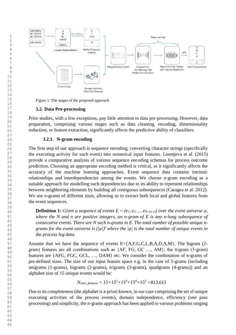
Figure 1. The stages of the proposed approach
3.2. Data Pre-processing
Prior studies, with a few exceptions, pay little attention to data pre-processing. However, data
preparation, comprising various stages such as data cleaning, encoding, dimensionality
reduction, or feature extraction, significantly affects the predictive ability of classifiers.
3.2.1. N-gram encoding
The first step of our approach is sequence encoding, converting character strings (specifically
the executing activity for each event) into numerical input features. Leontjeva et al. (2015)
provide a comparative analysis of various sequence encoding schemas for process outcome
prediction. Choosing an appropriate encoding method is critical, as it significantly affects the
accuracy of the machine learning approaches. Event sequence data contains intrinsic
relationships and interdependencies among the events. We choose n-gram encoding as a
suitable approach for modelling such dependencies due to its ability to represent relationships
between neighboring elements by building all contiguous subsequences (Caragea et al. 2012).
We use n-grams of different sizes, allowing us to extract both local and global features from
the event sequences.
Definition 1: Given a sequence of events E = (e1, e2,…, eN+(n-1)) over the event universe φ,
where the N and n are positive integers, an n-gram of E is any n-long subsequence of
consecutive events. There are N such n-grams in E. The total number of possible unique n-
grams for the event universe is (|φ|)n where the |φ| is the total number of unique events in
the process log data.
Assume that we have the sequence of events E=A,F,G,C,L,B,A,D,A,M. The bigram (2-
gram) features are all combinations such as AF, FG, GC …, AM; the trigram (3-gram)
features are AFG, FGC, GCL, …, DAM etc. We consider the combination of n-grams of
pre-defined sizes. The size of our input feature space e.g. in the case of 5-grams (including
unigrams (1-grams), bigrams (2-grams), trigrams (3-grams), quadgrams (4-grams)) and an
alphabet size of 15 unique events would be:
Ntotal_features = 15+152+153+154+155 =813,615
Due to its completeness (the alphabet is a-priori known, in our case comprising the set of unique
executing activities of the process events), domain independence, efficiency (one pass
processing) and simplicity, the n-grams approach has been applied to various problems ranging
1 2 3 4 5 6 7 8 9 10 11 12 13 14 15 16 17 18 19 20 21 22 23 24 25 26 27 28 29 30 31 32 33 34 35 36 37 38 39 40 41 42 43 44 45 46 47 48 49 50 51 52 53 54 55 56 57 58 59 60 61 62 63 64 65

from protein classification to information retrieval (Tomović et al. 2006). N-gram event data
requires no additional preprocessing such as sequence alignment. The letter n-grams method is
also very effective due to its ability to not only encode the letters but also order them
automatically. However, as seen in the above example, the size of generated input feature set
for classification problems tends to be very large: The number of features increases
exponentially with the n-gram length. Using all generated features directly would lead to
extremely high computational costs and the sparsity of the input would lead to reduced
accuracy. To address this challenge, we adopt a dimensionality reduction technique, feature
hashing, to reduce the size of n-gram feature vectors.
3.2.2. Feature Hashing
Feature hashing is an effective dimensionality reduction method that maps a high dimensional
input space into a low dimensional space (Weinberger et al. 2009). Feature hashing has found
successful applications in natural language processing (NLP), such as news categorization,
spam filtering, sentiment analysis in social networks and different areas of bioinformatics
(Forman and Kirshenbaum 2008; Ganchev and Dredze 2008; Caragea et al. 2012; Da Silva et
al. 2014). The main idea of feature hashing is to use hash functions to map n-grams of events
to feature vectors, which can be used to train the classifier.
Definition 2: Given a set of hashable features N, which are the n-grams obtained from the
process event sequences, h is the first hash function, h:N 1,……, m and ξ is the second
hash function, ξ:N ±1. The combined feature hashing function Φ(ℎ,𝜉)
maps the high
dimensional input vector of size d into a low-dimensional feature vector m where m < d.
The i-th element of the Φ(ℎ,𝜉)
(x) is given as: Φ𝑖(ℎ,𝜉)
(𝑥) = ∑ 𝜉(𝑗)𝑥𝑗𝑗:ℎ(𝑗)=𝑖 where j=0,…, d
and i=0,…., m.
Feature hashing not only reduces the training computational costs due to the reduced feature
dimensionality but also conserves memory. However, dimensionality reduction via feature
hashing can lead to information loss due to hash collisions, i.e. the mapping of many n-grams
to the same hash keys. Larger hash tables, i.e. larger bit sizes of the hash function, can prevent
this problem (Weinberger et al. 2009). Bit size determines the numbers of the bits when
creating the hash table. The optimal bit size depends on the size of the n-gram vocabulary. A
descriptive analysis of the n-grams obtained from the process sequences shows that they follow
Zipf’s law (Evermann et al. 2017). This implies that a small proportion of the input features
occur with higher frequencies. Hence, hash collisions are likely to take place for infrequent
variables and will incur low information loss (Caragea et al. 2012). The phenomenon can also
be observed in protein sequence classification problems (Caragea et al. 2012). As a reasonable
trade-off between dimensionality reduction and information loss, we use the 32 bit
murmurHash function (Langford et al. 2007) as hash function h,. The binary hash function ξ
is included to ensure that the hash kernel is unbiased (Weinberger et al. 2009).
3.3. Deep Learning Model
Artificial neural networks (ANN) offer a number of advantages over alternative machine
learning approaches for supervised learning tasks, including less need for formal statistical
modelling, the ability to detect complex non-linear relationships between predictors and
outcomes, the ability to model the interrelationships among the predictor variables, and the
availability of a range of training algorithms (Tu 1996). The superior performance of ANN has
1 2 3 4 5 6 7 8 9 10 11 12 13 14 15 16 17 18 19 20 21 22 23 24 25 26 27 28 29 30 31 32 33 34 35 36 37 38 39 40 41 42 43 44 45 46 47 48 49 50 51 52 53 54 55 56 57 58 59 60 61 62 63 64 65

been documented in many comparative empirical studies and competitions (Caruana and
Niculescu-Mizil 2006; Caruana et al. 2008; Schmidhuber 2015).
The traditional approach to train ANNs, particularly deep neural networks with multiple hidden
layers, directly optimizes the loss function through stochastic gradient descent, beginning from
randomly initialized weights. However, this results in long training durations and reduced
prediction performance (Vincent et al. 2010). Beginning in the mid-2000s offered more
effective training methods (Hinton et al. 2006; Vincent et al. 2008), such as deep belief network
(DBN), (stacked) autoencoders, denoised (stacked) autoencoders, have been developed. The
training process for these network architectures consists of two stages: (i) unsupervised greedy,
layerwise pre-training and (ii) supervised fine-tuning. The main idea of the unsupervised pre-
training is to address the need for learning complicated functions that represent high-level
abstractions. Network weights are obtained through self-supervised learning that learns the
non-linear transformation of the original input. The weights obtained from this stage are then
used for training the whole network. The supervised fine-tuning component maps the output
data to the pre-trained deep neural network and tries to minimize classification errors with
gradient-based optimization by adjusting the previously learned weights.
An extensive experimental study showed that neural networks with unsupervised pre-training
provide better classification results than networks without: The unsupervised pre-training
yields a good initial marginal distribution, captures intrinsic dependencies between variables,
outperforms classical regularization techniques, and acts as a variance reduction technique
(Erhan et al. 2010). We apply stacked autoencoders to extract high-level feature representation
layerwise in an unsupervised manner. After pre-training with stacked autoencoders, we
perform the fine-tuning and relevant classifications using a logistic regression layer after
adding an output layer to the obtained stack (see the Figure 2).
3.3.1. Unsupervised Pre-training with Stacked Autoencoders
Autoencoders are the non-linear generalization of the Principal Component Analysis (PCA)
that can model non-linear interdependencies among features (Hinton and Salakhutdinov 2006).
An autoencoder consists of three layers, namely input, hidden and output layers. The hidden
layer is referred to as encoding layer while the output layer acts as a decoding layer.
Encoder: The encoder maps the high-dimensional input vector x ∈ [0, 1]d to the hidden layer
using a non-linear activation function 𝑓𝜃. Due to its tendency to increase sparsity and reduced
tendency of vanishing gradients (Izadyyazdanabadi et al. 2017; Shi and Chu 2017), we adopted
the Rectified Linear Unit (ReLU) as an activation function for encoding:
ℎ = 𝑓𝜃(𝑥) = ReLU(𝑊𝑥 + 𝑏) (1)
θ = W, b is the parameter set of the encoder where W is a d′×d weight matrix and b is the
bias. h ∈ [0, 1]d is the output of the hidden layer representation.
Decoder: The decoder maps the hidden layer representation back to the reconstructed vector z
∈ [0, 1]d through the mapping function gϴ’.
𝑧 = 𝑔𝜃′(ℎ) = 𝑔𝜃′(𝑊′ℎ′ + 𝑏′) (2)
1 2 3 4 5 6 7 8 9 10 11 12 13 14 15 16 17 18 19 20 21 22 23 24 25 26 27 28 29 30 31 32 33 34 35 36 37 38 39 40 41 42 43 44 45 46 47 48 49 50 51 52 53 54 55 56 57 58 59 60 61 62 63 64 65

The main goal of the training is the optimization of parameter sets θ = W, b in the encoder
and θ’=W’,b’ in the decoder to minimize the reconstruction loss. We used squared error as
the reconstruction loss function L:
𝐿(𝑥, 𝑧) = ‖𝑥 − 𝑧‖2 = ‖𝑥 − 𝑔(𝑊′(𝑓(𝑊𝑥 + 𝑏) + 𝑏′)‖2 (3)
This optimization problem was solved using the mini batch stochastic gradient descent method.
Stacked autoencoders are a greedy layer-wise approach which conducts multi-phase feature
extraction by using the features extracted by one autoencoder, represented by its hidden layer,
as input of another, following autoencoder (left side of Figure 2) The stacked autoencoders are
trained independently to obtain the initial weights for the next stage, supervised fine-tuning. In
our study, we deploy an undercomplete autoencoder (a network architecture with the
decreasing width of hidden layers) to address the process prediction problem.
3.3.2. Supervised Fine-Tuning
After unsupervised reconstruction based learning of the network weights, logistic regression is
applied to fine-tune the weights after mapping the output to class labels (right side of Figure
2). For this, the decoding parts of the stacked autoencoders are removed and the logistic
regression layer is added on top of the trained encoding layers. Since we deal with a multi-class
classification problem, the added layer uses Softmax (multinomial logistic regression) units to
estimate the probabilities of the classes:
𝑃(𝑦 = 𝑗|𝑥) = 𝑒
𝜃𝑗
∑ 𝑒𝜃𝑖𝑘𝑖=1
(4)
The probability of the target class y being class j, given the input x, is calculated from the input
vector x and a set of weighting vectors 𝑤𝑗, where 𝜃𝑗 = 𝑤𝑗𝑇𝑥 denotes the inner product of 𝑤𝑗
and x. The combined network is trained using usual multi-layer perceptrons to minimize the
prediction error. We use stochastic gradient descent (SGD) to minimize the cost function. A
lock-free methodology was adopted to parallelize the SGD where the multiple cores contribute
to gradient updates (LeCun et al. 2012; Goodfellow et al. 2013).
Figure 2 Stacked autoencoders based deep learning. Unsupervised pre-training on the left, supervised fine-
tuning on the right.
1 2 3 4 5 6 7 8 9 10 11 12 13 14 15 16 17 18 19 20 21 22 23 24 25 26 27 28 29 30 31 32 33 34 35 36 37 38 39 40 41 42 43 44 45 46 47 48 49 50 51 52 53 54 55 56 57 58 59 60 61 62 63 64 65

4. Evaluation
To gauge the effectiveness of the proposed deep learning, we conducted a range of experiments
with different datasets, experimental settings and evaluation purposes. We investigated the
following research questions:
RQ1: Does the proposed multi-stage deep learning approach provide superior results
for different evaluation measures compared to existing classification approaches?
RQ2: Does the proposed multi-stage deep learning approach outperform the LSTM
based approaches by Evermann et al. (2017) and Tax et al. (2017) and the probabilistic
finite automaton (PFA) based on Bayesian regularization by Breuker et al. (2016)?
The third contribution of this study is to use data balancing to improve classification accuracy
(cf. Section 1). Business processes may contain rare activities that are not on the typical
execution path. This leads to imbalanced event logs, where some events are highly prevalent
and others are only sparsely represented, which are a challenge for classifier training. However,
rare activities are highly relevant in a business context as they may signal process exceptions,
process escalation or compensation tasks. Hence, it is important for classifiers to correctly
classify or predict rare events and we are therefore ask the following research question:
RQ3: Can process prediction with a multi-stage deep learning approach benefit from
data balancing to improve the prediction performance for rare process events? Because
traditional resampling techniques lead to overfitting, and the lack of information for
cost-sensitive learning, we use Radial Basis Function (RBF) neural networks to balance
the data. The ability of this approach to enhance the classification performance has
already been documented (Robnik-Šikonja 2014).
Our experiments were performed on an Intel i7-5500U 2.0 GHz processor with 16 GB RAM.
For data pre-processing, we used the dplyr package for R (Wickham and Francois 2015). We
developed a Java-based application to build the n-grams from the process event data. Feature
hashing was done on the Microsoft Azure ML platform using the Vowpal Wabbit library
(Langford et al. 2007; Barga et al. 2015). Both the pre-trained, stacked autoencoders and the
supervised deep learning part were created on the H20 open source deep learning platform
(Candel et al. 2016). We used Weka (Hall et al. 2009) for experiments with traditional
classifiers.
4.1. Datasets
The experiments used real-life datasets, the BPI Challenge 2012 (van Dongen 2012), BPI
Challenge 2013 (W. Steeman 2013), and Helpdesk (Verenich 2016) data. Table 1 describes the
datasets. The number of unique event types is the number of output classes in our multi-class
classification problem.
The BPI Challenge 2012 dataset comprises 262000 events for 13087 cases, obtained from a
Dutch financial institute. The activities related to a loan application process are categorized
into three sub-processes: activities related to the application (A), activities belonging to
applications (W) and activities related to the offer (O). Events for the A and O sub-processes
contain only the completion lifecycle transition, while the W process includes the scheduled,
1 2 3 4 5 6 7 8 9 10 11 12 13 14 15 16 17 18 19 20 21 22 23 24 25 26 27 28 29 30 31 32 33 34 35 36 37 38 39 40 41 42 43 44 45 46 47 48 49 50 51 52 53 54 55 56 57 58 59 60 61 62 63 64 65

started and completed lifecycle transitions. As Evermann et al. (2017), Breuker et al. (2016),
and Tax et al. (2017) use only the completion events, we remove the started and scheduled
events from this sub-process. Similar to the previous papers, we evaluate our approach on three
datasets from BPI Challenge 2012: BPI_2012_A, BPI_2012_O and BPI_2012_W_Completed.
The BPI Challenge 2013 dataset contains log data from an incident and problem management
system of Volvo IT in Belgium. It has three subsets: The incident management subset
encompasses 7554 cases with 65533 events of 13 unique types. The open problems subset
contains 819 cases with 2351 events of 5 unique types, and the closed problems subset
comprises 1487 cases with 6660 events of 7 unique types. We merged the open and closed
problems subsets to create a dataset identical to that in other studies, yielding 9011 events.
The helpdesk dataset comprises event data from a ticketing management system designed for
the help desk of an Italian software company. The event log contains 3804 cases with 13710
events.
The BPI Challenge 2012 data provides both organizational information such as the
identification number of the resources initiating events, and case specific information such as
the amount of the requested loan. The BPI Challenge 2013 datasets contain information about
the priority of the problems and incidents, originating functional divisions and organizational
lines, related products, process owners’ countries and names. After generating the feature
vectors from the sequence of the activities through n-grams and feature hashing approaches,
we appended the additional information from the logs to the feature vector.
Table 1 Characteristics of dataset
Datasets # of unique event types # of events
BPI_2012_W_Completed 6 72413
BPI_2012_A 10 60849
BPI_2012_O 7 31244
BPI_2013_Incidents 13 65533
BPI_2013_Problems 7 9011
Helpdesk 9 13710
4.2. Evaluation Metrics
To evaluate the effectiveness of our deep learning approach and to compare it to other
classification algorithms, we computed average accuracy, averaged precision, average recall,
average F-measure, and Matthews Correlation Coefficient (MCC) and the area under the ROC
curve (AOC) (see the Table 2), which were adapted to a multi-class classification problem.
In these formulas, tpi (true positives for class i) is the number of events of class i that have been
classified or predicted as being of class i. fpi (false positives) is the number of events not of
class i that have been classified (predicted) as being of class i. tni (true negative) is the number
of events not of class i that have been classified (predicted) as not of class i and finally fni (false
negatives) is the number of events of class i that have been classified (predicted) as not of class
i. tpri is the true positive rate and fpri the false positive rate for class i. Accuracy is defined as
the proportion of correctly predicted instances of all instances. Precision determines how many
activities were correctly classified for a particular class, given all predictions of that class.
1 2 3 4 5 6 7 8 9 10 11 12 13 14 15 16 17 18 19 20 21 22 23 24 25 26 27 28 29 30 31 32 33 34 35 36 37 38 39 40 41 42 43 44 45 46 47 48 49 50 51 52 53 54 55 56 57 58 59 60 61 62 63 64 65

Recall is the true positive rate for a particular class. The F-Measure is the harmonic weighted
mean of precision and recall. MCC is referred as the correlation between the target values and
predicted classifications. AUC is the area under the ROC (receiver operating characteristic)
curve. We computed these measures for each individual class and obtained the overall value
by summing up their scores, weighted by the true class size.
Table 2 Evaluation metrics for multi-class classification. l is the number of classes, 𝑠𝑖 is the true size of class i
(the number of events of class i) and 𝑛 = ∑ 𝑠𝑖𝑙𝑖=1 is the total size of the dataset.
Metrics Formula
Accuracy 1
𝑛∑ 𝑠𝑖
𝑡𝑝𝑖 + 𝑡𝑛𝑖
𝑡𝑝𝑖 + 𝑓𝑛𝑖 + 𝑡𝑛𝑖 + 𝑓𝑝𝑖
𝑙
𝑖=1
Precision 1
𝑛∑ 𝑠𝑖
𝑡𝑝𝑖
𝑡𝑝𝑖 + 𝑓𝑝𝑖
𝑙
𝑖=1
Recall 1
𝑛∑ 𝑠𝑖
𝑡𝑝𝑖
𝑡𝑝𝑖 + 𝑓𝑛𝑖
𝑙
𝑖=1
F-Measure 1
𝑛∑ 𝑠𝑖
𝑝𝑟𝑒𝑐𝑖𝑠𝑖𝑜𝑛𝑖 × 𝑟𝑒𝑐𝑎𝑙𝑙𝑖
𝑝𝑟𝑒𝑐𝑖𝑠𝑖𝑜𝑛𝑖 + 𝑟𝑒𝑐𝑎𝑙𝑙𝑖
𝑙
𝑖=1
MCC 1
𝑛∑ 𝑠𝑖
𝑡𝑝𝑖 × 𝑡𝑛𝑖 − 𝑓𝑝𝑖 × 𝑓𝑛𝑖
√(𝑡𝑝𝑖 + 𝑓𝑝𝑖)(𝑡𝑝𝑖 + 𝑓𝑛𝑖)(𝑡𝑛𝑖 + 𝑓𝑝𝑖)(𝑡𝑛𝑖 + 𝑓𝑛𝑖)
𝑙
𝑖=1
AUC 1
𝑛∑ 𝑠𝑖 ∫ 𝑡𝑝𝑟𝑖 𝑑(𝑓𝑝𝑟𝑖)
1
0
𝑙
𝑖=1
80% of each dataset was used for training and 20% for testing. The test results were used to
compare the approaches. We used the training data for both unsupervised pre-training and
supervised fine tuning of our deep learning model. We used 10-fold cross validation for
training, in which the dataset is partitioned into the 10 disjoint subsets. Both training and testing
are carried out 10 times. During each iteration, one subset is used for testing whereas the others
are used for training the classifier. This procedure is important for identifying the best
hyperparameter configuration (Vincent et al. 2010).
4.3. Hyperparameter Optimization
Deep neural networks may have more than fifty hyperparameter (Bergstra et al. 2011).
Hyperparameter optimization significantly affects the learning process and prediction
outcomes by identifying the best parameter configuration from the given hyperparameter space
at a reasonable computational cost. In the traditional approach, manual search, experts define
some hyperparameter values for different parameters based on their experience and intuitions
(such as the number of hidden layers, the number of neurons, the learning rate etc.) and try to
find the best combination of hyperparameter values by conducting multiple training sessions.
Due to the time consuming nature of this approach, only a few hyperparameter value
combinations can be tested (Bergstra et al. 2011). Furthermore, due to the shortcomings of
human reasoning in multi-dimensional spaces, it is challenging to achieve globally optimal
outcomes (Witt and Seifert 2017).
The brute force, exhaustive approach (grid search), trains the model for every possible
combination of hyperparameter values by following some stopping criterion. Grid search
identifies better hyperparameter configuration than manual search in the same computational
time (Bergstra and Bengio (2012)). Most deep learning studies use a combination of manual
and grid search, where experts define the possible values for each variable and grid search then
1 2 3 4 5 6 7 8 9 10 11 12 13 14 15 16 17 18 19 20 21 22 23 24 25 26 27 28 29 30 31 32 33 34 35 36 37 38 39 40 41 42 43 44 45 46 47 48 49 50 51 52 53 54 55 56 57 58 59 60 61 62 63 64 65

finds the best combination of these (Larochelle et al. 2007). Such an exhaustive search suffers
from the “curse of the dimensionality” since the number of combinations increases
exponentially with the number of hyperparameters (Bergstra et al. 2011). To address this,
Bergstra and Bengio (2012) proposed a random search approach. The idea is to pick
combinations of hyperparameter values randomly and to train the models in the given
constraint (e.g. compute time). Empirical results show that random search outperforms the
brute-force grid search (Bergstra and Bengio 2012).
Hence, we adopt the random search hyperparameter optimization approach. We defined the
parameter ranges for number of hidden layers [3:10], number of neurons in the hidden layers
[10:500] considering the undercomplete network structure, sparse data handling [True, False],
initial weight distribution [uniform, normal] for the pre-training component, number of training
epochs [10:1000], adaptive learning rate (adaptive learning rate time decay factor=0.99 and
adaptive learning rate smoothing factor = 1e-8), (initial) learning rate [0.0001:1], annealing rate
[10:106] when adaptive learning is disabled, for both pre-training component and the whole
network. We stopped the search when 200 models for a given dataset are trained. Training is
stopped early if relative improvement is below a defined threshold. We used log-loss as the
early stopping metric with a threshold of 0.001. Table 3 shows the optimal hyperparameter
configuration for the BPI_2012_A dataset. We performed hyperparameter optimization for all
our experiments but do not show optimal values due to space restrictions.
Table 3 Optimal hyperparameter values for BPI Challenge 2012_A dataset
4.4. Results
The following subsections provide discuss our experimental results to address our research
questions. All reported results are from the test data subset.
4.4.1. Comparative Analysis (RQ 1 and RQ 2)
We first compared our approach to conventional (i.e. generic or not-process aware)
classification algorithms including support vector machines (SVM), random forests, naïve
Bayes, k-nearest-neighbours (kNN) and C4.5 decision trees, which are among the most
Parameters (pre-training) Values Parameters (whole Network) Values
Number of Neurons (hidden
layers) 425:400:390:300 Number of layers 6 (4 hidden)
Initial Weight Distribution Normal
distribution Epochs 100
Sparse True Adaptive Learning True
Learn Rate 0.005 Adaptive learning rate smoothing
factor 1e-8
Momentum 0.9 Adaptive learning rate time decay
factor 0.99
Annealing Rate 104
Activation ReLu
Activation (classification) Softmax
Batch size 20
classifier L2-penalty 0
Loss Function Cross-
entropy
1 2 3 4 5 6 7 8 9 10 11 12 13 14 15 16 17 18 19 20 21 22 23 24 25 26 27 28 29 30 31 32 33 34 35 36 37 38 39 40 41 42 43 44 45 46 47 48 49 50 51 52 53 54 55 56 57 58 59 60 61 62 63 64 65

powerful and most widely-used algorithms (Wu et al. 2008). Table 4 presents our results for
predicting the next event for prefix length 5, n-gram size 3 and bit size 10.
The results for different performance measures show that, with few exceptions, our approach
outperforms conventional, generic classification methods. The SVM method performs better
than other methods over all three datasets and comes closest to our approach. For the BPI 2013
dataset, all methods except naïve Bayes perform similarly. The performance gaps between our
approach and the alternative methods are quite large for the BPI 2012 and helpdesk datasets.
Table 4 Results obtained from conventional classification approaches and the proposed deep learning approach
(higher numbers are better)
Accuracy Precision Recall F-Score MCC AUC
BPI 2012_A
SVM 0.817 0.856 0.822 0.817 0.748 0.895
RF 0.720 0.714 0.721 0.712 0.566 0.888
Naïve Bayes 0.612 0.633 0.612 0.555 0.485 0.772
C4.5 0.708 0.744 0.709 0.705 0.674 0.931
Deep Learning 0.824 0.852 0.824 0.817 0.751 0.923
BPI2013_Incidents
SVM 0.652 0.599 0.653 0.622 0.350 0.730
RF 0.615 0.626 0.616 0.524 0.508 0.895
Naïve Bayes 0.576 0.618 0.577 0.590 0.519 0.879
C4.5 0.659 0.558 0.659 0.582 0.564 0.900
Deep Learning 0.663 0.648 0.664 0.647 0.583 0.862
Helpdesk
SVM 0.715 0.605 0.716 0.652 0.389 0.725
RF 0.601 0.619 0.601 0.606 0.278 0.688
Naïve Bayes 0.631 0.634 0.631 0.622 0.323 0.733
C4.5 0.613 0.534 0.614 0.569 0.214 0.602
Deep Learning 0.782 0.632 0.781 0.711 0.412 0.762
In summary, to answer RQ1, we observe that our proposed deep learning approach is superior
to conventional, generic classification methods.
To examine RQ2, we compared our approach to three recent approaches for next event
prediction. The results for all three BPI 2012 datasets show that our approach outperforms all
three approaches (see the Table 5). A bigger difference can be observed for the
BPI_2012_W_Completed dataset, where our approach achieves an accuracy of 0.831
compared to 0.719 in Breuker et al. (2016) and 0.760 in Tax et al. (2017). The performance
gap compared to Breuker et al. (2016) is greatest for recall (sensitivity). The comparison of our
results with Evermann et al. (2017) in terms of precision also shows the superior performance
of our proposed approach (0.811 vs. 0.658). Only two other studies used the BPI_2012_A and
BPI_2012_O datasets to evaluate their models. Our approach outperforms both of those models
in terms of all evaluation measures. The approach by Evermann et al. (2017) performs better
for the latter two and achieves results close to ours.
The results for the BPI_2013_Incident dataset are mixed. The approach in Breuker et al. (2016)
shows higher predictive performance than ours in terms of accuracy (0.714 vs. 0.663).
However, our approach performs significantly better in terms of recall (0.664 vs. 0.377).
Precision results obtained in Evermann et al. (2017) are also better than for our approach.
1 2 3 4 5 6 7 8 9 10 11 12 13 14 15 16 17 18 19 20 21 22 23 24 25 26 27 28 29 30 31 32 33 34 35 36 37 38 39 40 41 42 43 44 45 46 47 48 49 50 51 52 53 54 55 56 57 58 59 60 61 62 63 64 65

However, the experiments conducted on the BPI_2013_Problems dataset suggest that our
approach delivers superior results compared to the alternatives.
Finally, only Tax et al. (2017) carried out experiments on the helpdesk data. Our approach
performs better than LSTM approach in terms of accuracy (0.782 vs. 0.712).
We also note that, since we use the random hyperparameter optimization instead of a manual
search as in our previous study (Author citation, 2017), the results presented here are a
significant improvements over own earlier work (Author citation, 2017), demonstrating the
importance of this step.
In summary, to answer RQ2, we conclude that our approach outperforms existing deep-
learning process prediction approaches for most datasets and on most quality metrics.
Table 5 Comparison against benchmark approaches (higher numbers are better)
We examined the effect of the n-gram size on prediction accuracy. Since most process traces
in the BPI_2012 and Helpdesk datasets contain less than 6 events, we defined the maximum
length of prefix and n-grams as 5. For the BPI_2013 we were able to build 10-grams. The
experiment results suggest that increasing the size of the n-grams (from 2 to 5 and 10) does not
lead to significant changes in the predictive capability of the model, while using longer n-grams
increases computational costs. For example, the accuracy on the BPI2012_A and a prefix
length of 5 ranges between 0.829 and 0.831 for n-grams sizes between 2 and 5, showing little
improvement.
We also investigated the effect of the bitsize of the feature hashing on accuracy. As mentioned
above, hash collisions can be reduced by increasing the bitsize of the hash table. Our results
Accuracy Precision Recall
BPI 2012_W
Breuker et al. (2016) 0.719 - 0.578
Evermann et al. (2017) - 0.658 -
Tax et al. (2017) 0.760 - -
Proposed Approach 0.831 0.811 0.832
BPI2012_A
Breuker et al. (2016) 0.801 - 0.723
Evermann et al. (2017) 0.832 -
Proposed Approach 0.824 0.852 0.824
BPI2012_O
Breuker et al. (2016) 0.811 - 0.647
Evermann et al. (2017) - 0.836
Proposed Approach 0.821 0.847 0.822
BPI2013_Incidents
Breuker et al. (2016) 0.714 - 0.377
Evermann et al. (2017) - 0.735
Proposed Approach 0.663 0.648 0.664
BPI2013_Problems
Breuker et al. (2016) 0.690 - 0.521
Evermann et al. (2017) - 0.628
Proposed Approach 0.662 0.641 0.662
Helpdesk
Tax et al. (2017) 0.712 - -
Proposed Approach 0.782 0.632 0.781
1 2 3 4 5 6 7 8 9 10 11 12 13 14 15 16 17 18 19 20 21 22 23 24 25 26 27 28 29 30 31 32 33 34 35 36 37 38 39 40 41 42 43 44 45 46 47 48 49 50 51 52 53 54 55 56 57 58 59 60 61 62 63 64 65

show that increasing the bitsize beyond a certain threshold does not improve prediction results.
In our case, this threshold was 10. This can be explained by the fact that the frequency of n-
grams obtained from the process event sequences follow Zipf’s law, which states that only a
small proportion of the input features occur with higher frequencies (Caragea et al. 2012). This
implies that the majority of hash collisions take place for infrequent, and thus less important,
n-grams.
4.4.2. Imbalanced Classification (RQ 3)
In unbalanced datasets, some classes are severely underrepresented compared to others. This
reduces the effectiveness of the machine learning techniques, especially for detecting the
minority class examples (Wang and Yao 2012). To overcome this, various approaches at the
data level (randomly or informatively under/over sampling), algorithm level, cost sensitive
learning and boosting methods have been proposed (Sun et al. 2009). Due to their simple
nature, resampling approaches are used frequently, but they are unable to increase the
information that is required to train the models. Furthermore, undersampling may result in
information loss. The SMOTE (Synthetic Minority Over-sampling Technique) method was
proposed to address this issue. It generates new, non-replicated samples by interpolating
neighboring minority class examples, but it also suffers from synthesizing noisy examples
(Huang et al. 2016). Cost sensitive learning techniques are effective approaches to tackle the
imbalanced classification problem but require cost information from domain experts. Huang et
al. (2016) suggests that applying neural networks to synthesize the samples for minority class
is a superior alternative.
In our study, we generate semi-artificial data of the minority class using Radial Basis Function
(RBF) neural networks (Robnik-Šikonja 2014). This approach extracts Gaussian kernels from
the RBF trained with dynamic decay adjustment, and generates data from each kernel in the
required proportions. Details and pseudo-code of the RBF based data generator can be found
in (Robnik-Šikonja 2014). We chose RBF networks for their advantages over other data
generation methods. Although other methods consider the relationship between input and target
variables, they do not consider dependencies among input variables. Such dependencies are
preserved in the RBF based model. The RBF method assumes only the form of the data
distribution (Gaussian), but uses extracted distribution parameters to generate data.
The process owners of the BPI Challenge 2013 Incidents dataset claim that employees try to
find workarounds to stop the clock in order to manipulate the resolution time of an incident.
Giving an incident a status of “Wait user” is one of these ways. Although employees were
explicitly requested to avoid using the status of “Wait user” except for emergency cases, the
guideline is occasionally broken. Identifying this misuse is therefore highly business relevant.
However, this event occurs very infrequently. To handle this imbalanced classification
problem, we reformulate the problem as a binary classification problem where the majority
class is the set of all other events and the minority class is the “Wait user” event. We then apply
our approach after balancing the class occurrence frequencies with the RBF method. We
compare the results against the direct application of our approach to the imbalanced data
(without rebalancing). Accuracy is inappropriate for comparing classification results for
imbalanced datasets. Even when a classifier detects all majority examples correctly and fails
1 2 3 4 5 6 7 8 9 10 11 12 13 14 15 16 17 18 19 20 21 22 23 24 25 26 27 28 29 30 31 32 33 34 35 36 37 38 39 40 41 42 43 44 45 46 47 48 49 50 51 52 53 54 55 56 57 58 59 60 61 62 63 64 65

to predict the examples from the minority class, the accuracy will still be high due to the
prevalence of majority class examples (Han et al. 2005). Instead, we used the area under the
ROC curve (AUC), which is an appropriate measure of the performance for imbalanced data
(Bradley 1997). Figure 3 shows ROC curves for the imbalanced data and for the RBF
rebalanced data.
Figure 3 ROC Curves for application to (a) imbalanced and (b) balanced datasets. ROC curves plot the true
positive rate (tpr) against the false positive rate (fpr).
The results show that balancing the dataset through RBF based data generation imrpoves the
accuracy of our approach positively by increasing the AUC from 0.855 to 0.932.
In summary, to answer RQ3, we conclude that RBF based data rebalancing works well in
conjunction with our proposed multi-level deep learning prediction approach to improve the
prediction of rare, but important, events in a business process.
5. Discussion and Conclusion
This paper investigated the effectiveness of a stacked autoencoders based deep learning
approach for predicting future process events of a running process instance. It is the first
application of this approach in the business process prediction domain. To evaluate the
predictive performance of our method, we compared it against three recent approaches, two of
which used LSTM recurrent neural networks, and conventional classification algorithms.
Before applying the deep learning model, we used n-gram encoding and feature hashing to
build numerical feature vectors from categorical process event data using a sliding window
technique. The research objective was to examine the feasibility and impact of applying the
proposed approach to process prediction. The experimental results suggest that the proposed
method achieves good results on different evaluation metrics and outperforms the state-of-the-
art approaches in most experiments. We also investigated and discussed the effect of adjusting
the hyperparameter of the data pre-processing stage and the deep neural networks on the
prediction results and applied hyperparameter optimization to find the optimal configuration.
Finally, we addressed the imbalanced classification problem by employing neural-network
based resampling methods.
In addition to its superior predictive performance, the proposed deep learning approach offers
other advantages over conventional techniques. Unsupervised pre-training of neural networks
with stacked autoencoders is useful in the presence of unlabeled data as it is able to learn a
good feature representation from unlabeled data in a self-supervised manner. Moreover,
1 2 3 4 5 6 7 8 9 10 11 12 13 14 15 16 17 18 19 20 21 22 23 24 25 26 27 28 29 30 31 32 33 34 35 36 37 38 39 40 41 42 43 44 45 46 47 48 49 50 51 52 53 54 55 56 57 58 59 60 61 62 63 64 65

undercomplete (a deep neural networks architecture with decreasing width (layer sizes) hidden
layers) stacked autoencoders can construct useful higher-level feature representations in their
layers and thus reduce the feature dimensionality. These higher-level feature representations
are useful for other problems in the business process management domain that rely on event
trace features, such as case based reasoning problems, process instance similarity search,
process instance clustering, process instance retrieval, etc.
Another contribution of this study is the investigation of the advantages provided by data-
preprocessing. We have shown the importance of n-grams based encoding of the sequential
business process data. In contrast, the majority of prior approaches use simple indexing, which
ignores sequential interdependencies among the events and results in relatively low
classification performance. We have also shown the importance of data reduction techniques
such as feature hashing, which significantly accelerate the classification algorithms. This is
particularly important for real-time predictions required for automating process decisions.
This study deals with predicting the next activities in the given process trace. Knowing the
occurrence probabilities of the next events allows decision makers to dynamically optimize
process execution by adjusting resource allocation, rescheduling process activities, changing
activities or taking appropriate actions outside the process instance. Alternatively, by predicting
the occurrence of an undesired event, the system warns managers and allows them to avoid it
proactively.
The successful application of our proposed approach to next event prediction opens up
interesting and important avenues for future work. Our method can also be applied to predicting
business process outcomes, such as compliance with service-level agreements, process success
or failure. Even if there is no need for algorithmic changes, business process outcome
prediction requires intensive feature processing work. Using denoised stacked autoencoders
may improve the pre-training results over the ones used here, and is also a subject of future
research. Finally, applying the proposed multi-stage deep learning approach to regression
problems, such as time to next event or remaining time to case completion, is another
interesting research question. By combining the next event prediction with other process driven
analytics such as activity duration estimation, it is possible to address more complicated
decision tasks.
Our approach, like other predictive methods, assumes that the process (and its event log data)
is in a steady state. This means that the relationship between input and output does not change
over time and a model trained with historical data can be used to predict new data instances.
The results on our experimental datasets show this assumption to be valid at least for these
datasets. However, it is reasonable to believe that changes may occur in the control-flow
(behavioral), resource and data perspectives of the business processes (Bose et al. 2011).
Referred also to as concept drift, these changes may be recurring, sudden, gradual and
incremental (Bose et al. 2011). It is important to consider this issue when designing and training
a model for predictive business process monitoring. In the data preparation phase of our
approach, we already adopt the sliding windows technique for creating the dataset to train our
algorithm. With a slight adjustment to the current training procedure, e.g. by forgetting old data
upon the arrival new data instances (fixed window approach) and retraining the proposed model
iteratively, we can obtain a basic model that is able to handle concept drift. In future work, we
1 2 3 4 5 6 7 8 9 10 11 12 13 14 15 16 17 18 19 20 21 22 23 24 25 26 27 28 29 30 31 32 33 34 35 36 37 38 39 40 41 42 43 44 45 46 47 48 49 50 51 52 53 54 55 56 57 58 59 60 61 62 63 64 65

intend to address feature drift, concept drift, and changing prior distributions by combining our
deep learning approach with methods that handle these different aspects of concept drift.
Finally, expert knowledge and relevant cost information is an important issue when evaluating
the performance of classifiers. Evaluating whether an accuracy of 80% (as in BPI 2012 case in
this study) is reasonable for adopting the classification models depends on several factors such
as the characteristics of application domain, the nature of underlying process, and the legal and
financial consequences of misclassification. Classification in this context is a decision making
process which combines predictions with utility/cost functions to attain the goal defined by
analysts. Different decision makers have different risk tolerances and consequently different
utility functions. Hence, the utility functions determine the acceptable performance of
probabilistic machine learning approaches. In future research, we aim to integrate our
predictive analytics approach with the decision making process in a real world use-case.
We also aim to provide post-hoc explanations to address the “black-box” nature of deep-
learning methods and make their predictions interpretable to domain experts. This is important
to establish trust in the model results. Incorporating automated decision making for process
monitoring in EIS (e.g. triggering alerts upon detection of process execution) requires an
understanding of the underlying model, as does using the predictive analytics based on PAIS
data for decision making in knowledge intensive processes where the humans are the final
decision makers. Our future research aims make process prediction models more
understandable.
References
Author Citation (2017)
Barga R, Fontama V, Tok WH, Cabrera-Cordon L (2015) Predictive analytics with Microsoft Azure machine
learning. Apress, 2015
Bergstra J, Bengio Y (2012) Random Search for Hyper-Parameter Optimization. Journal of Machine Learning
Research 13:281–305.
Bergstra JS, Bardenet R, Bengio Y, Kégl B (2011) Algorithms for hyper-parameter optimization. In: Advances
in Neural Information Processing Systems. pp 2546–2554
Bose RPJC, van der Aalst WMP, Žliobaitė I, Pechenizkiy M (2011) Handling concept drift in process mining.
In: International Conference on Advanced Information Systems Engineering. Springer, pp 391–405
Bradley AP (1997) The use of the area under the ROC curve in the evaluation of machine learning algorithms.
Pattern Recognition 30:1145–1159.
Breuker D, Matzner M, Delfmann P, Becker J (2016) Comprehensible Predictive Models for Business
Processes. Management Information Systems Quarterly 40:1009–1034.
Candel A, Parmar V, LeDell E, Arora A (2016) Deep learning with h2o. H2O Inc
Caragea C, Silvescu A, Mitra P (2012) Protein sequence classification using feature hashing. Proteome Science
10:1–14.
Caruana R, Karampatziakis N, Yessenalina A (2008) An empirical evaluation of supervised learning in high
dimensions. In: Proceedings of the 25th International Conference on Machine learning. ACM, pp 96–103
Caruana R, Niculescu-Mizil A (2006) An empirical comparison of supervised learning algorithms. In:
Proceedings of the 23rd international conference on Machine learning. ACM, pp 161–168
Da Silva NFF, Hruschka ER, Hruschka ER (2014) Tweet sentiment analysis with classifier ensembles. Decision
Support Systems 66:170–179.
Davenport TH, Harris JG (2007) Competing on analytics : the new science of winning, 1st edn. Harvard
Business School Press
Di Francescomarino C, Dumas M, Federici M, et al (2016) Predictive business process monitoring framework
with hyperparameter optimization. In: International Conference on Advanced Information Systems
Engineering. Springer, pp 361–376
Duan L, Da Xu L (2012) Business intelligence for enterprise systems: a survey. IEEE Transactions on Industrial
Informatics 8:679–687.
Erhan D, Bengio Y, Courville A, et al (2010) Why Does Unsupervised Pre-training Help Deep Learning?
1 2 3 4 5 6 7 8 9 10 11 12 13 14 15 16 17 18 19 20 21 22 23 24 25 26 27 28 29 30 31 32 33 34 35 36 37 38 39 40 41 42 43 44 45 46 47 48 49 50 51 52 53 54 55 56 57 58 59 60 61 62 63 64 65

Journal of Machine Learning Research 11:625–660.
Evermann J, Rehse J-R, Fettke P (2017) Predicting process behaviour using deep learning. Decision Support
Systems 100:129–140.
Folino F, Guarascio M, Pontieri L (2012) Discovering context-aware models for predicting business process
performances. In: OTM Confederated International Conferences“ On the Move to Meaningful Internet
Systems.” Springer, pp 287–304
Forman G, Kirshenbaum E (2008) Extremely fast text feature extraction for classification and indexing. In:
Proceedings of the 17th ACM conference on Information and knowledge management. ACM, pp 1221–
1230
Ganchev K, Dredze M (2008) Small statistical models by random feature mixing. In: Proceedings of the ACL08
HLT Workshop on Mobile Language Processing. pp 19–20
Goodfellow IJ, Warde-Farley D, Mirza M, et al (2013) Maxout networks. arXiv preprint arXiv:1302.4389
Gregor S, Hevner AR (2013) Positioning and presenting design science research for maximum impact.
Management Information Systems Quarterly 37:337–356.
Hall M, Frank E, Holmes G, et al (2009) The WEKA data mining software: an update. ACM SIGKDD
Explorations Newsletter 11:10–18.
Han H, Wang W-Y, Mao B-H (2005) Borderline-SMOTE: a new over-sampling method in imbalanced data sets
learning. Advances in Intelligent Computing 878–887.
Hinton GE, Osindero S, Teh Y-W (2006) A fast learning algorithm for deep belief nets. Neural Computation
18:1527–1554.
Hinton GE, Salakhutdinov RR (2006) Reducing the dimensionality of data with neural networks. science
313:504–507.
Huang C, Li Y, Change Loy C, Tang X (2016) Learning deep representation for imbalanced classification. In:
Proceedings of the IEEE Conference on Computer Vision and Pattern Recognition. pp 5375–5384
Izadyyazdanabadi M, Belykh E, Mooney M, et al (2017) Convolutional Neural Networks: Ensemble Modeling,
Fine-Tuning and Unsupervised Semantic Localization for Intraoperative CLE Images.
https://arxiv.org/pdf/1709.03028
Kang B, Kim D, Kang S (2012a) Periodic performance prediction for real‐ time business process monitoring.
Industrial Management & Data Systems 112:4–23.
Kang B, Kim D, Kang S-H (2012b) Real-time business process monitoring method for prediction of abnormal
termination using KNNI-based LOF prediction. Expert Systems with Applications 39:6061–6068.
Lakshmanan GT, Shamsi D, Doganata YN, et al (2015) A markov prediction model for data-driven semi-
structured business processes. Knowledge and Information Systems 42:97–126.
Langford J, Li L, Strehl A (2007) Vowpal wabbit online learning project.
Larochelle H, Erhan D, Courville A, et al (2007) An empirical evaluation of deep architectures on problems
with many factors of variation. In: Proceedings of the 24th International Conference on Machine learning.
ACM, pp 473–480
LaValle S, Lesser E, Shockley R, et al (2011) Big data, analytics and the path from insights to value. MIT Sloan
Management Review 52:21.
Le M, Gabrys B, Nauck D (2017) A hybrid model for business process event and outcome prediction. Expert
Systems 34:e12079.
Le M, Nauck D, Gabrys B, Martin T (2014) Sequential Clustering for Event Sequences and Its Impact on Next
Process Step Prediction. In: International Conference on Information Processing and Management of
Uncertainty in Knowledge-Based Systems. Springer, pp 168–178
LeCun YA, Bottou L, Orr GB, Müller K-R (2012) Efficient backprop. In: Neural networks: Tricks of the trade.
Springer, pp 9–48
Leontjeva A, Conforti R, Di Francescomarino C, et al (2015) Complex symbolic sequence encodings for
predictive monitoring of business processes. In: International Conference on Business Process
Management. Springer, pp 297–313
Márquez-Chamorro AE, Resinas M, Ruiz-Cortés A, Toro M (2017) Run-time prediction of business process
indicators using evolutionary decision rules. Expert Systems With Applications 87:1–14.
Metzger A, Leitner P, Ivanovic D, et al (2015) Comparing and Combining Predictive Business Process
Monitoring Techniques. IEEE Transactions on Systems, Man, and Cybernetics: Systems 45:276–290.
Polato M, Sperduti A, Burattin A, de Leoni M (2016) Time and Activity Sequence Prediction of Business
Process Instances. http://arxiv.org/abs/1602.07566
Robnik-Šikonja M (2014) Data generator based on RBF network. arXiv preprint arXiv:1403.7308
Rogge-Solti A, Weske M (2013) Prediction of remaining service execution time using stochastic petri nets with
arbitrary firing delays. In: International Conference on Service-Oriented Computing. Springer, pp 389–
403
Schmidhuber J (2015) Deep learning in neural networks: An overview. Neural Networks 61:85–117.
1 2 3 4 5 6 7 8 9 10 11 12 13 14 15 16 17 18 19 20 21 22 23 24 25 26 27 28 29 30 31 32 33 34 35 36 37 38 39 40 41 42 43 44 45 46 47 48 49 50 51 52 53 54 55 56 57 58 59 60 61 62 63 64 65

Senderovich A, Di Francescomarino C, Ghidini C, et al (2017) Intra and inter-case features in predictive process
monitoring: A tale of two dimensions. In: International Conference on Business Process Management.
Springer, pp 306–323
Shi S, Chu X (2017) Speeding up Convolutional Neural Networks By Exploiting the Sparsity of Rectifier Units.
https://arxiv.org/pdf/1704.07724
Sun Y, Wong AKC, Kamel MS (2009) Classification of imbalanced data: A review. International Journal of
Pattern Recognition and Artificial Intelligence 23:687–719.
Sun Z, Pambel F, Wang F (2015) Incorporating Big Data Analytics into Enterprise Information Systems. In:
Information and Communication Technology: Third IFIP TC 5/8 International Conference, ICT-EurAsia
2015, and 9th IFIP WG 8.9 Working Conference, CONFENIS 2015. Springer, pp 300–309
Tax N, Verenich I, La Rosa M, Dumas M (2017) Predictive Business Process Monitoring with LSTM Neural
Networks. In: International Conference on Advanced Information Systems Engineering. pp 477–492
Tomović A, Janičić P, Kešelj V (2006) n-Gram-based classification and unsupervised hierarchical clustering of
genome sequences. Computer Methods and Programs in Biomedicine 81:137–153.
Tu J V. (1996) Advantages and disadvantages of using artificial neural networks versus logistic regression for
predicting medical outcomes. Journal of Clinical Epidemiology 49:1225–1231.
Unuvar M, Lakshmanan GT, Doganata YN (2016) Leveraging path information to generate predictions for
parallel business processes. Knowledge and Information Systems 47:433–461.
van der Aalst WMP, Schonenberg MH, Song M (2011) Time prediction based on process mining. Information
Systems 36:450–475.
van Dongen BF (2012) BPI Challenge 2012. https://doi.org/10.4121/uuid:3926db30-f712-4394-aebc-
75976070e91f
van Dongen BF, Crooy RA, van der Aalst WMP (2008) Cycle time prediction: When will this case finally be
finished? In: OTM Confederated International Conferences“ On the Move to Meaningful Internet
Systems.” Springer, pp 319–336
Verenich I (2016) Helpdesk. 10.17632/39bp3vv62t.1, 2016.
Vincent P, Larochelle H, Bengio Y, Manzagol P-A (2008) Extracting and composing robust features with
denoising autoencoders. In: Proceedings of the 25th International Conference on Machine learning. ACM,
pp 1096–1103
Vincent P, Larochelle H, Lajoie I, et al (2010) Stacked Denoising Autoencoders: Learning Useful
Representations in a Deep Network with a Local Denoising Criterion. Journal of Machine Learning
Research 11:3371–3408.
W. Steeman (2013) BPI Challenge 2013. https://doi.org/10.4121/uuid:a7ce5c55-03a7-4583-b855-98b86e1a2b07
Wang S, Yao X (2012) Multiclass imbalance problems: Analysis and potential solutions. IEEE Transactions on
Systems, Man, and Cybernetics, Part B (Cybernetics) 42:1119–1130.
Weinberger K, Dasgupta A, Langford J, et al (2009) Feature hashing for large scale multitask learning. In:
Proceedings of the 26th Annual International Conference on Machine Learning - ICML ’09. ACM Press,
pp 1–8
Wickham H, Francois R (2015) dplyr: A grammar of data manipulation. R package version 04 1:20.
Witt N, Seifert C (2017) Understanding the Influence of Hyperparameters on Text Embeddings for Text
Classification Tasks. In: International Conference on Theory and Practice of Digital Libraries. Springer,
pp 193–204
Wu X, Kumar V, Quinlan JR, et al (2008) Top 10 algorithms in data mining. Knowledge and Information
Systems 14:1–37.
XES Standard (2016) 1849-2016 - IEEE Standard for eXtensible Event Stream (XES) for Achieving
Interoperability in Event Logs and Event Streams. http://www.xes-standard.org/.
1 2 3 4 5 6 7 8 9 10 11 12 13 14 15 16 17 18 19 20 21 22 23 24 25 26 27 28 29 30 31 32 33 34 35 36 37 38 39 40 41 42 43 44 45 46 47 48 49 50 51 52 53 54 55 56 57 58 59 60 61 62 63 64 65

Process Event Sequence
ABCDEFG
BCLKENF
BCLKEND
……………..
EBCDDAG
n-grams Representation
A
B
BC
ABCD
……………..
CDEFG
Hashed Sequence
Features
0
1
1234
……………..
33
Supervised Fine-Tuning
with Logistic Regression
Feature Hashing
Process Logs
Merged Feature Vector
wTx
Unsupervised
Pre-Training with
Stacked Autoencoders
A
B
C
D
……………..
Z
Next Process Event
Resource Features
Data Flow Features
Deep Learning
Figure 1 The stages of the proposed approach
Figure 1 updated

𝑋1
𝑋2
𝑋3
𝑋4
𝑋5
𝑋6
𝑋7
𝑋𝑛
+1
ℎ1(1)
ℎ2(1)
ℎ3(1)
ℎ4(1)
ℎ𝑚(1)
+1
𝑋1
𝑋2
𝑋3
𝑋4
𝑋5
𝑋6
𝑋7
𝑋8
ℎ1(1)
ℎ2(1)
ℎ3(1)
ℎ4(1)
ℎ𝑚(1)
+1
ℎ1(2)
ℎ2(2)
ℎ𝑘(2)
+1
ℎ1(1)
ℎ2(1)
ℎ3(1)
ℎ4(1)
ℎ5(1)
ℎ6(1)
Features I Output Input(Feature I)
Features II Output
Unsupervised Pre-training with Stacked Autoencoders Supervised Fine-tuning with Logistic Regression
Original
Input
𝑋1
𝑋2
𝑋3
𝑋4
𝑋5
𝑋6
𝑋7
𝑋𝑛
+1
ℎ1(1)
ℎ2(1)
ℎ3(1)
ℎ4(1)
ℎ𝑚(1)
+1
ℎ1(2)
ℎ2(2)
ℎ𝑘(2)
+1
Original
InputFeatures I
(pre-trained)
Features II
(pre-trained)
Softmax Layer
(P(y=1x)
(P(y=2x)
(P(y=3x)
Figure 2 Stacked autoencoders based deep learning. Unsupervised pre-training on the left, supervised fine-tuning on the right.
Figure 2 updated

AUC = 0.855
a. Results for imbalanced dataset b. Results for balanced dataset
AUC = 0.932
Figure 3 ROC Curves for application to (a) imbalanced and (b) balanced datasets. ROC curves plot the true positive rate (tpr) against the false positive rate (fpr).
Figure 3

Table 1 Characteristics of dataset
Datasets # of unique event types # of events
BPI_2012_W_Completed 6 72413
BPI_2012_A 10 60849
BPI_2012_O 7 31244
BPI_2013_Incidents 13 65533
BPI_2013_Problems 7 9011
Helpdesk 9 13710
Table 2 Evaluation metrics for multi-class classification. l is the number of classes, 𝑠𝑖 is the true size of class i
(the number of events of class i) and 𝑛 = ∑ 𝑠𝑖𝑙𝑖=1 is the total size of the dataset.
Metrics Formula
Accuracy 1
𝑛∑ 𝑠𝑖
𝑡𝑝𝑖 + 𝑡𝑛𝑖
𝑡𝑝𝑖 + 𝑓𝑛𝑖 + 𝑡𝑛𝑖 + 𝑓𝑝𝑖
𝑙
𝑖=1
Precision 1
𝑛∑ 𝑠𝑖
𝑡𝑝𝑖
𝑡𝑝𝑖 + 𝑓𝑝𝑖
𝑙
𝑖=1
Recall 1
𝑛∑ 𝑠𝑖
𝑡𝑝𝑖
𝑡𝑝𝑖 + 𝑓𝑛𝑖
𝑙
𝑖=1
F-Measure 1
𝑛∑ 𝑠𝑖
𝑝𝑟𝑒𝑐𝑖𝑠𝑖𝑜𝑛𝑖 × 𝑟𝑒𝑐𝑎𝑙𝑙𝑖
𝑝𝑟𝑒𝑐𝑖𝑠𝑖𝑜𝑛𝑖 + 𝑟𝑒𝑐𝑎𝑙𝑙𝑖
𝑙
𝑖=1
MCC 1
𝑛∑ 𝑠𝑖
𝑡𝑝𝑖 × 𝑡𝑛𝑖 − 𝑓𝑝𝑖 × 𝑓𝑛𝑖
√(𝑡𝑝𝑖 + 𝑓𝑝𝑖)(𝑡𝑝𝑖 + 𝑓𝑛𝑖)(𝑡𝑛𝑖 + 𝑓𝑝𝑖)(𝑡𝑛𝑖 + 𝑓𝑛𝑖)
𝑙
𝑖=1
AUC 1
𝑛∑ 𝑠𝑖 ∫ 𝑡𝑝𝑟𝑖 𝑑(𝑓𝑝𝑟𝑖)
1
0
𝑙
𝑖=1
Tables

Table 3 Optimal hyperparameter values for BPI Challenge 2012_A dataset
Table 4 Results obtained from conventional classification approaches and the proposed deep learning approach
(higher numbers are better)
Accuracy Precision Recall F-Score MCC AUC
BPI 2012_A
SVM 0.817 0.856 0.822 0.817 0.748 0.895
RF 0.720 0.714 0.721 0.712 0.566 0.888
Naïve Bayes 0.612 0.633 0.612 0.555 0.485 0.772
C4.5 0.708 0.744 0.709 0.705 0.674 0.931
Deep Learning 0.824 0.852 0.824 0.817 0.751 0.923
BPI2013_Incidents
SVM 0.652 0.599 0.653 0.622 0.350 0.730
RF 0.615 0.626 0.616 0.524 0.508 0.895
Naïve Bayes 0.576 0.618 0.577 0.590 0.519 0.879
C4.5 0.659 0.558 0.659 0.582 0.564 0.900
Deep Learning 0.663 0.648 0.664 0.647 0.583 0.862
Helpdesk
SVM 0.715 0.605 0.716 0.652 0.389 0.725
RF 0.601 0.619 0.601 0.606 0.278 0.688
Naïve Bayes 0.631 0.634 0.631 0.622 0.323 0.733
C4.5 0.613 0.534 0.614 0.569 0.214 0.602
Deep Learning 0.782 0.632 0.781 0.711 0.412 0.762
Parameters (pre-training) Values Parameters (whole Network) Values
Number of Neurons (hidden
layers) 425:400:390:300 Number of layers 6 (4 hidden)
Initial Weight Distribution Normal
distribution Epochs 100
Sparse True Adaptive Learning True
Learn Rate 0.005 Adaptive learning rate smoothing
factor 1e-8
Momentum 0.9 Adaptive learning rate time decay
factor 0.99
Annealing Rate 104
Activation ReLu
Activation (classification) Softmax
Batch size 20
classifier L2-penalty 0
Loss Function Cross-
entropy

Table 5 Comparison against benchmark approaches (higher numbers are better)
Accuracy Precision Recall
BPI 2012_W
Breuker et al. (2016) 0.719 - 0.578
Evermann et al. (2017) - 0.658 -
Tax et al. (2017) 0.760 - -
Proposed Approach 0.831 0.811 0.832
BPI2012_A
Breuker et al. (2016) 0.801 - 0.723
Evermann et al. (2017) 0.832 -
Proposed Approach 0.824 0.852 0.824
BPI2012_O
Breuker et al. (2016) 0.811 - 0.647
Evermann et al. (2017) - 0.836
Proposed Approach 0.821 0.847 0.822
BPI2013_Incidents
Breuker et al. (2016) 0.714 - 0.377
Evermann et al. (2017) - 0.735
Proposed Approach 0.663 0.648 0.664
BPI2013_Problems
Breuker et al. (2016) 0.690 - 0.521
Evermann et al. (2017) - 0.628
Proposed Approach 0.662 0.641 0.662
Helpdesk
Tax et al. (2017) 0.712 - -
Proposed Approach 0.782 0.632 0.781