Embed Size (px)
Citation preview
1
TIMING OR TARGETING: THE ASYMMETRIC MOTIVES OF CAPITAL
STRUCTURE DECISIONS
Islam Abdeljawad
Fauzias Mat Nor
Graduate School of Business
Universiti Kebangsaan Malaysia
Email: [email protected]
Abstract
This study investigates how the timing behavior and the adjustment towards the target of
capital structure interact in the capital structure decisions. Past literature finds that both
timing and targeting are significant in determining the leverage ratio which is inconsistent
with any standalone framework. This study argues that the coexistence of both timing and
targeting is possible. The preference of the firm for timing behavior or targeting behavior
depends on the cost of deviation from the target. Since the cost of deviation from the
target is likely to be asymmetric between overleveraged and underleveraged firms, the
direction of the deviation from the target leverage is expected to alter the preference
toward timing or targeting in the capital structure decision. Using GMM-system
estimators with the Malaysian data for the period of 1992-2009, this study finds that
Malaysian firms, on average, adjust their leverage at a slow speed of 12.7% annually
increased to 14.2% when the timing variable is accounted for. Moreover, the speed of
adjustment is found to be significantly higher and the timing role is lower for
overleveraged firms compared with underleveraged firms. Overleveraged firms seem to
find less flexibility to time the market as more pressure is exerted on them to return to the
target regardless the timing opportunities because of the higher costs of deviation from
the target leverage. Underleveraged firms place lower priority to rebalance toward the
target compared with overleveraged firms as the costs of being underleveraged is lower
and hence, they have more flexibility to time the market. The findings of this study
support that tradeoff theory and timing theory are not mutually exclusive. Firms consider
both targeting and timing in their financing decisions but the preference of one motive
over the other is conditional on the cost of the deviation from the target.
KEYWORDS: Market timing theory, Tradeoff theory, Dynamic capital structure, Speed
of adjustment, GMM system
1. INTRODUCTION
Equity market timing and tradeoff theories get an increasing interest in the capital
structure literature for the entire last decade. Market timing theory (Baker and Wurgler,
2002) suggests that firms can recognize times of mispricing of their own stock and time
their issuing (repurchasing) activity accordingly. In this theory, firms are indifferent
toward any target leverage and no steady adjustment toward any target should be noticed.
Instead, changes in leverage are largely dominated by successive timing activities. On the
other hand, the trade-off theory include a family of models, both static and dynamic, in
2
which firms attempt to balance the advantages against the costs associated with
borrowing by keeping the leverage ratio at a certain target level (Baxter, 1967; Jensen
and Meckling, 1976; Leary and Roberts 2005). In the dynamic version of trade-off
theory, any deviation from the target leverage is costly and requires a quick action to
adjust to the target.
One important aspect that can differentiate between the timing and trade-off theories is
by the estimation of the speed of adjustment (SOA) toward the target (Huang and Ritter,
2009). While tradeoff theory expects high SOA, timing theory expects, basically, no
adjustment. The other aspect for differentiating between the two theories is that trade-off
theory is built on rational expectation assumption; mispricing is not expected to play a
role as a capital structure determinant while it is the main determinant in timing theory.
However, literature find that both timing and targeting motives actually exist at the same
time which depart from the prediction of any standalone theory (Graham and Harvey,
2001; Huang and Ritter, 2009; Kayhan and Titman, 2007). How the two motives interact
in the decision making process remains largely unknown. Moreover, recent literature
indicates that adjustment behavior is not homogenous across firms i.e. no single SOA can
fit all firms. A more reasonable approach to investigate the adjustment behavior is to use
multiple SOA’s (Clark et al., 2009; Flannery and Hankins, 2007; Lemmon et al., 2008).
Whether the firm is overleveraged or underleveraged is one of the aspects that are found
to affect the SOA (Clark et al., 2009; Lemmon et al., 2008). Overleveraged firms are
found to have high SOA compared with underleveraged firms. The asymmetry in the
SOA is interpreted as a result of the asymmetry in the costs of deviation from the target
(Flannery and Hankins, 2007).
This study will investigate the adjustment behavior of Malaysian firms and how the
accounting for timing behavior affects this adjustment behavior. Moreover, this study
will investigate if targeting and timing behaviors are mutually exclusive as theoretically
expected or they can coexist. Given that the adjustment behavior depends on the
difference between the cost of deviation and the cost of adjustment and that the cost of
deviation is higher for overleveraged firms than underleveraged firms, the benefits of
timing are more likely to outweigh the net cost of deviation for underleveraged firms
more than that of overleveraged firms. Firms that are above the target will put higher
priority to adjust than to exploit timing opportunities. For firms that are underleveraged,
adjusting may not be a priority and firms are more likely to exploit the timing
opportunities as they appear. This timing asymmetry is likely to continue in the long run
since the firm is less active rebalance the short run timing effect once it is underleveraged
compared with being overleveraged. The findings of Baker and Wurgler (2002) that
timing activities drive the leverage ratio may be specific to underleveraged firms if this
hypothesis holds.
The findings of this research will add more insight to the capital structure dynamics. The
suggested interaction between timing behavior and targeting behavior in determining the
capital structure of the firm is new. This study contributes to the literature by shedding
light on one possible interpretation for the otherwise apparent as contradicted results in
the past literature. The new interpretation proposes that the two motives of timing and
targeting are likely to coexist, but with different weights for firms above and below the
3
target. While overleveraged firms are more likely to adjust faster, the underleveraged
firms are expected to be better timers. This asymmetric behavior of timing is a result of
the asymmetry of the costs and benefits associated with both motives. Moreover, this
study will address the estimation problems highlighted in previous literature by using
GMM system approach of Blundell and Bond (1998) which is found to be less biased
than other estimators in the case of weak instruments, short time dimension and large
number of cross-sections as typically the case of capital structure research. This estimator
is recent to the Malaysian capital structure research and the results may improve the
understanding of the way firms make financing decisions.
2. BACKGROUND
Adjustment towards the target leverage is a behavior expected by a set of capital structure
theories that assume the existence of a target leverage and that the deviation from the
target is costly. Examples of these theories include tradeoff theory (Baxter, 1967; Kraus
and Litzenberger, 1973), agency theory (Jensen and Meckling, 1976) and free cash flow
theory (Jensen, 1986). Extant literature generally supports the existence of long-run target
leverage and agrees on the notion that a typical firm adjust to that target gradually at a
certain SOA but the magnitude of this SOA is not a settled issue (Frank and Goyal,
2007). Extreme finding of high SOA of about 80% yearly is found by de Miguel and
Pindado (2001) while no adjustment is found by Baker and Wurgler (2002). Alti (2006)
and Flannery and Rangan (2006) both documented a relatively rapid SOA which they
interpreted in favor of tradeoff theory. In contrast, Fama and French (2002) and Kayhan
and Titman (2007) find only slow SOA which indicates that tradeoff factors may be only
secondary aspects in the capital structure decisions.
In timing theory, leverage ratio is driven solely by the mispricing of the firm’s equity,
whether real or just perceived by the managers of the firm. Timing theory assumes that
the firm is indifferent toward any level of leverage since no target is assumed. Obviously,
this theory departs from the rational expectation assumption to allow the mispricing of
equity to consistently affect the leverage ratio. The prediction of timing theory of capital
structure is supported internationally (Baker and Wurgler, 2002; Mahajan and Tartaroglu,
2008) and for Malaysia (Abdeljawad and Mat Nor, 2011).
If one motive drives the dynamism of capital structure, the effect of the other motives
will vanish once the right motive is accounted for properly (Flannery and Rangan, 2006).
However, current literature supports that both targeting and timing motives may coexist.
Survey evidence of Graham and Harvey (2001) find that both targeting and timing are
taken into consideration in the financing decisions. Managers consider the amount of
overvaluation or undervaluation as a key determinant in the decision to issue common
stock. Moreover, the increase in the price of common stock is found to be among the top
reasons for issuing common stock. At the same time, about 81% of the managers agreed
that they have some kind of target leverage. However, the target is strictly defined for
only 10% while 34% have a targeted range and another 37% have flexible target. The
survey findings of Graham and Harvey (2001) have been supported later by firm level
studies. Huang and Ritter (2009) find that firms finance larger amount of the financing
4
deficit using external equity when the cost of equity is lower. At the same time, they find
that firms adjust to the target at a rate of 17%. Kayhan and Titman (2007) find that stock
price history affects the debt ratio for about 10 years consistent with the timing theory.
However, part of this effect is gradually reversed since debt ratios tend to adjust toward
target debt ratio but at a slow rate.
The findings of these studies are hardly reconciled with one capital structure theory as
both timing and targeting are supported. This study proposes that timing and targeting are
not mutually exclusive. Timing benefits are opportunities to reduce the cost of equity by
an amount equal to the difference between the intrinsic value and the market value of the
stock. Each 1% of overvaluation of the stock issued leads to 1% reduction in the cost of
equity. The benefit of market timing can be considered as an additional factor in a broad
dynamic tradeoff framework. In the dynamic tradeoff framework, adjustment behavior
depends on the cost of deviation from the target and the costs of adjustments toward the
target. Adjustments take place only if the cost of deviation is larger than the cost of
adjustment so the net of these two costs drive the capital structure decisions (Leary and
Roberts, 2005). In the proposed framework, the benefits of timing are taken into account
in the capital structure decision as an additional factor that is offset with the net cost of
deviation. Assuming that the net cost of deviation is positive, if the benefit of timing is
higher than the net cost of deviation, the firm will exploit the timing opportunity. If the
net cost of deviation is larger than the timing benefit, the firm will adjust whatever the
market valuation of the firm is.
The adjustment behavior is not homogenous across all firms. The SOA varies across
firms directly with the variation in the costs and benefits of being at the target, for
instance the higher probability of distress leads to faster adjustments since it implies that
the cost of deviation is high (Flannery and Hankins, 2007; Clark et al. 2009). Past
literature finds that overleveraged firms face higher costs of deviation and should adjust
faster compared with underleveraged firms. The heterogeneity between firms that are
overleveraged and those are underleveraged is documented by (Clark et al., 2009;
Lemmon et al., 2008). This asymmetry in the SOA is interpreted as a result of the
asymmetry in the costs of deviation from the target where the costs of deviation are likely
to be higher for overleveraged firms than underleveraged firms.
The costs of deviation above the target include the increased probability of financial
distress which lead to higher borrowing rates and more restrains on new debt for
overleveraged firms. In addition, agency problems between debt-holders and
shareholders may be deepening for these firms (Jensen and Meckling, 1976; Myers,
1977). As a result, the total cost of deviation is expected to be high and to intensify
rapidly as the deviation above the target increases more.
Of course, there are costs to be underleveraged as well. The underleveraged firm may
lose the tax advantage of debt financing and it may lack the role of debt as a manager
disciplining device (Jensen, 1986). However, there is evidence that these costs are lesser
for underleveraged firms than overleveraged firms. The zero leverage phenomenon
studied by (Strebulaev and Yang, 2007) indicates that being underleveraged is not costly
5
to many firms. About 9% of all US firms over the period from 1962 to 2002 have zero
debt and almost one quarter of the firms have less than 5% debt. Moreover, the tax shield
substitutes may reduce the tax advantages of debt for many firms (DeAngelo and
Masulis, 1980). The costs of deviation below the target are then lower and increase
slowly as the deviation below the target increase compared to the rapid increase of the
costs associated with being overleveraged.
If the costs of deviation for overleveraged firms are higher than the costs for
underleveraged firms and the net cost of deviation is competing with the benefits of
timing in the decision making, then underleveraged firms are likely to exploit more
timing opportunities than overleveraged firms. Timing opportunities for underleveraged
firms can outweigh the net cost of deviation more often compared with overleveraged
firms. In sum, the firm will exploit more timing opportunities once it is underleveraged
and it will not rush to adjust toward the target after that since the cost of deviation from
the target is low. If the firm is overleveraged, it is more likely to have net cost of
deviation that is larger than the timing benefits; hence the firm will not exploit many
timing opportunities and will prefer to adjust even if favorable market conditions exist.
Based on this conjecture, this research suggests that the direction of the deviation from
the target, i.e. whether the firm is overleveraged or underleveraged, is one of the
determinants that are likely to moderate the behavior of timing versus targeting of the
firm. The SOA is expected to be higher for overleveraged firms and the timing will be
lower. Overleveraged firms will place higher priority on reducing their level of leverage
than on waiting for market timing opportunities. On the other hand, underleveraged firms
may find that the benefits of timing are higher than the cost of deviation from the target.
These firms will place lower priority to rebalance toward the target compared with
overleveraged firms and they are expected to have more flexibility to time the market,
hence the SOA is expected to be lower and market timing is expected to be more
pronounced.
The starting point for this research is to estimate the SOA for the full sample using GMM
system approach which is found to be less biased than other estimators of dynamic
models. Estimating the SOA is an investigation for whether the target considerations are
a first priority factors in capital structure decisions or they are just secondary factors.
Next, the research will investigate the effect of market valuation on the adjustment
behavior of the firm. Following Flannery and Rangan (2006), if timing behavior
dominates targeting behavior, it should wipe out the effect of targeting once it is
accounted for in the model. The factors associated with the dominant theory will appear
to be more important once both groups of factors are competing together. Lastly, this
research will investigate when the role of timing is likely to show up and when it will be
cool-off compared with tradeoff motives. Specifically, this research hypothesize that the
tradeoff versus timing motives are moderated by the direction of the deviation from the
target.
6
In the remaining of this paper, the methodology and models will be explained in Section
3. The data will be described in Section 4 and the descriptive statistics in Section 5.
Estimation results and discussion in Section 6 and finally, Section 7 will conclude.
3. METHODOLOGY
3.1. Variables
The dependent variable of this research is the leverage ratio of the firm. According to
Rajan and Zingales (1995), the most relevant definition of leverage depends on the
objective of the analysis. Measures like total liabilities to total assets can proxy for what
is left for shareholders in case of liquidation but not a good indication of the risk of
default that the firm faces since items that are used for transaction purposes rather than
for financing, like accounts payable, can overstate the amount of leverage. A more
relevant definition of leverage to this research is the total debt to total assets ratio which
reflects only the debt financing policy of the firm (Hovakimian, 2006).
Another issue is whether to use book values or market values in the definition of
leverage. Book leverage reflects the financing history of the firm while market leverage is
largely future oriented reflecting the market valuation of leverage ratio. Fama and French
(2002) argue that most predictions of tradeoff and pecking order models apply directly to
book leverage and some carry over to market leverage. Investigating the timing ability of
the firm is also more related to past financing activities since timing is an active reaction
to market opportunities. Shocks to market leverage can result either from active financing
decisions or simply from passive fluctuations resulted from stock price movements
(Welch, 2004). For timing behavior, only active financing transactions are relevant,
hence book leverage is likely to better capture these transactions.
Market timing variable should capture the relationship between market valuation of the
firm and leverage. The market valuation of the firm can be linked to mispricing through
the representativeness heuristic (Tversky and Kahneman, 1974). People tend to use the
last observation in a sequence as an anchor to make predictions (Bolger&Harvey 1993).
The proxy for timing is the stock price performance (SPP) defined as the difference in the
logarithm of price between two successive periods which is basically the stock return (De
Bie and De Haan, 2007; Deesomsak et al., 2004; Homaifar et al., 1994).
In addition to the timing variable, a set of control variables that are found to be
significant in past literature have been used. The control variables utilized in this research
are the ones that are found to be significant in Rajan and Zingales (1995) and
subsequently used by Baker and Wurgler (2002). These variables are also identified to be
the significant capital structure determinants in Malaysia (Booth et al., 2001). These
control variables are size, profitability, tangibility and growth options.
In a tradeoff context, the company size affects the capital structure because larger firms
tend to be more diversified and less prone to bankruptcy (Rajan and Zingales, 1995;
Titman and Wessels, 1988). Add to this, since part of the bankruptcy costs are fixed, it is
7
expected to find economies of scale in the bankruptcy costs. So, larger firms face lower
unit cost of bankruptcy which may encourage the use of more leverage. In addition,
agency costs of debt will be less with larger firms since bondholders are more likely to be
repaid for their money, and hence, the firm is likely to use more leverage. The proxy for
size in this research is the logarithm of sales, where sales are adjusted for inflation using
constant prices of 2005.
For profitability, Myers and Majluf (1984) argued that as a result of asymmetric
information, companies prefer internal sources of finance. In other words, higher
profitability companies tend to have lower debt levels. Relative to this theory Titman and
Wessels (1988) and Rajan and Zingales (1995) find leverage to be negatively related to
the level of profitability. Fama and French (2002) and Myers (1984) use this negative
relationship as evidence against the trade-off model. The proxy for profitability in this
research is the earnings before interest, taxes and depreciation to total assets.
Tradeoff theory suggests that tangibility affects the capital structure as the more tangible
the assets of a firm are, the greater the assets that can be used as collateral. Tangible
assets add more security to the debt and reduce losses associated with information
asymmetry. Consequently, a positive relationship is expected with the level of debt
finance (Rajan and Zingales, 1995). The proxy for tangibility is the property, plant and
equipment net of depreciation to total assets.
Growth opportunities are defined as “capital assets that add value to a firm but cannot be
collateralized and do not generate current taxable income” (Titman and Wessels, 1988).
Myers (1977) argued that due to information asymmetries, companies with high leverage
ratios might have the tendency to undertake activities that transfer wealth a way from
bondholders toward shareholders (under-invest in economically profitable projects and
asset substitution) and this will increase the agency costs of debt. Therefore, it can be
argued that companies with growth opportunities tend to use greater amount of equity
finance because they have stronger incentives to avoid underinvestment and asset
substitution that arise from stockholder-bondholder conflicts. Moreover, in the free cash
flow theory of Jensen (1986), growth firms have less free cash flow and less debt is
needed to be used as a control mechanism. In addition, growth options cannot be
collateralized, and hence, financial distress will be higher for firms with higher growth
leading these firms to use more equity. On the other hand, simple pecking order theory
posits a positive association between leverage and growth opportunities. In this
framework, a firm’s leverage should increase as investments opportunities exceed
retained earnings and vice versa. Thus, maintaining profitability level constant, funds
needed in excess of retained earnings, will be obtained from debt expecting higher
leverage for those firms with better growth opportunities. Empirical results are mixed.
For example, Bradley et al. (1984), Rajan and Zingales (1995) and Fama and French
(2002) find a negative relationship between leverage and growth opportunities while
Titman and Wessels (1988) did not find support to the effect of growth on leverage.
Booth et al. (2001) find a significant positive relationship for many developing countries
including Malaysia, Thailand, India and Turkey. The main proxy for growth is the market
to book ratio defined as total assets minus book equity plus market equity all divided by
8
total assets where market equity is the result of the product of the number of common
shares and the end of the year share price.
3.2. Models
In a dynamic adjustment model, if the costs of adjusting to the target leverage are zero,
the firm will always keep its leverage at the target by instantly counteract shocks.
However, in the presence of adjustment costs the firm will adjust only if the adjustment
costs are less than the costs of deviation from the target. A standard partial adjustment
model is usually used to capture this dynamism. The setup of the partial adjustment
model is
where is the average SOA and is the target leverage.
The model assumes that the firm has a target leverage that minimizes the cost of capital.
Nevertheless, shocks can make the firm deviates from the target. Once the firm is
deviated from the target, it should adjust as long as the cost of deviation is higher than the
cost of adjustment. According to the partial adjustment model, the actual adjustment in
leverage is some fraction of the desired adjustment for each period which is called the
SOA . If =1, it means that full adjustment occur each period, while if =0, no
adjustment takes place. The SOA should be a fraction between 0 and 1 if an adjustment
behavior is followed by the firm.
The target leverage is unobservable and hence proxied by the fitted value from a
regression of observed leverage on a set of firm characteristics identified in the previous
literature as important determinants of the target (Fama and French, 2002; Flannery and
Rangan, 2006; Hovakimian et al., 2001; Kayhan and Titman, 2007). The target in this
case changes from firm to firm and from year to year for the same firm as it is a function
of the firm characteristics. The fit value of Eq. (2) will be used as the target leverage.
Eq. (2)
where and are firm and time fixed effects and other variables are self explanatory.
However, estimation of the partial adjustment model can be done by incorporating the
target leverage (Eq. (2)) into the partial adjustment model (Eq. (1)) and rearranging the
terms. Then, the estimation can be done in a single step using Eq. (3)
Eq. (3)
where the SOA equals one minus the coefficient of the lagged leverage. is the set
of control variables all used as concurrent regressors, except for the lagged leverage, to
allow for more observations to be used. The firm and time fixed effects are accounted for
in the model following (Flannery and Rangan, 2006; Lemmon et al., 2008).
9
To investigate the effect of market timing on the adjustment process, a regression that
includes the timing variable as well as the other variables that’s supposed to determine
the target leverage will be used. Flannery and Rangan (2006) argue that if timing
behavior can dominate the targeting behavior, the timing variable should be able to wipe
out the influence of targeting behavior once it is added to the model. Following Flannery
and Rangan (2006), the following model will be used to investigate the effect of timing
behavior on the targeting behavior:
Eq. (4) is similar to Eq. (3) except that a timing variable is added to the model. The
benchmark that will be used for comparison is Eq. (3). If adding the timing variable
reduces the estimated coefficients of and the SOA significantly, that mean that timing
variable has dominated the tradeoff forces.
Lastly, this research has controlled for the direction of the deviation from the target by
dividing the sample based on whether the firm is over or underleveraged and re-estimate
Eq. (3) and Eq. (4) for the two sub-samples then compare the results. Since instrumental
variables are used in the estimation, separating the two groups aims to insure that the
instruments used for estimation are from the same group not the other group. To create
the subsamples, the deviation from the target is calculated first based on the following
relationship
If the deviation is positive (negative), the firm is overleveraged (underleveraged). The
target leverage is a function of firm characteristics hence; it varies across firm and time.
Since leverage value is, by definition, bounded by minimum 0 and maximum 1, any fit
value for the target leverage that is out of the sample observations is replaced by its actual
value to be consistent with the defined boundaries.
3.3. Econometrics approach
The estimation of Eq. (3) and Eq. (4) raises many econometric issues. Mainly, the lagged
leverage regressor is likely to be endogenous because it arises within a system that
influences the error term. To obtain consistent estimators for this model, instrumental
variables should be used to account for endogeneity problem. The instruments should
satisfy the two requirements
i. Exogeneity requirement which mean no correlation between the instrument and the
error is exists. This requirement leads to instrument validity.
ii. Relevance requirement which mean a high correlation of the instrument and the
endogenous regressor should be satisfied.
The instrumental variable estimators are consistent once the instruments are valid. If the
instruments are only marginally relevant, they are called weak instruments. In case of
weak instruments, estimators are still consistent but may provide poor approximation to
actual sampling distribution. The challenge is then to find the appropriate instruments.
10
An increasingly popular approach for estimation of dynamic models is the difference
generalized methods of moments (difference GMM) of Arellano and Bond (1991). The
difference GMM is able to account for the unobservable time invariant variables by using
the first difference of the variables. Moreover, GMM is able to mitigate the endogeneity
problem by using the instrumental variable approach where the lags in level of the
endogenous variable are used as instruments.
The main drawback of GMM difference is that it has poor finite sample properties in case
that the instruments are weak. If the time series are persistent, the number of periods are
short and the number of cross sections are large the lagged levels are likely to be only
weak instruments for subsequent first differences (Blundell and Bond, 1998).
Unfortunately, these features typically exist in the case of capital structure studies
(Lemmon et al., 2008). Therefore, GMM difference may result in imprecise or even
biased estimators in this case.
An alternative to GMM difference is the GMM system of Arellano and Bover (1995) and
Blundell and Bond (1998) where two simultaneous equations are estimated; one in the
level and the other in the first difference. The lagged level of the endogenous variable is
used to instrument the first difference equation and the differenced variable is used to
instrument the level equation. The GMM system estimator is found to be more efficient
and has less finite sample bias due to the exploitation of more moment conditions
especially when the instruments are weak. Recently, many papers have utilized the
system GMM in estimating the dynamic capital structure models (Antoniou et al., 2008;
Clark et al., 2009; Lemmon et al., 2008). Lemmon et al. (2008) argue that system GMM
is expected to produce large efficiency gains over other approaches that use difference
GMM or two-stage least square methods. This research will employ the GMM system in
estimation.
This study uses orthogonal deviation to get rid of the firm fixed effects (Arellano and
Bover, 1995). In this method, the average of all future available observations of the
variable is subtracted from each observation. This type of deviation is able to remove the
fixed effect and is computable for all the observations except the last one for each firm
(Roodman, 2006). Since the lagged observation is not included in the orthogonal
deviation, the resulted deviations are available as valid instruments as well. The use of
orthogonal deviations is preferable in the case that many gaps exist in the unbalanced
panel data which is likely to occur once the two subsamples are created while the first
differencing transformation is likely to magnify the number of gaps and may affect the
estimated coefficients. Time fixed effects are captured by including year dummies to
remove the effect of general time-related shocks (e.g. macroeconomic shocks common to
all firms) from the error term as recommended by Roodman (2006) and Ozkan (2001).
The instruments used for the leverage endogenous variable, in all models, are the lagged,
level and difference, two periods and earlier, up to the end of the available time series of
the firm. Other variables are assumed to be exogenous and hence they instrument
11
themselves. All GMM models are estimated using robust two-step estimation method and
standard errors are corrected using Windmeijer (2005) finite sample correction.
3.4. Model Diagnostics
It is expected for GMM estimators to have first order autocorrelation, but the crucial
requirement for GMM estimators to be consistent is the absence of second order
autocorrelation. If second order autocorrelation exists, some lags are invalid instruments
and should be removed from the instrument set. Both first order autocorrelation and
second order autocorrelation developed by Arellano and Bond (1991) are reported in this
research. In addition, instruments must be exogenous to be valid. Otherwise, the moment
conditions will not be satisfied. A test for the validity of the over-identifying restrictions
called “Hansen test” is used in this research. The null hypothesis for this test is that “all
instruments are valid”. This is a null that should not be rejected in order to proceed with
GMM estimation. The rejection of the null indicates that at least one of the instruments is
not valid.
Lastly, Wald test indicates that the model well fit the data. The null hypothesis of this test
is that the set of coefficients of the model are simultaneously equal to zero. If the null
cannot be rejected, the variables of the model are not doing good job in predicting the
dependent variable.
4. DATA
The data of this research include all firms available in Thomson Financial Worldscope
Database1 for the Malaysian market during the period of 1992-2009. Data before 1992 is
often missing and hence, returning earlier than that year is not feasible. Financial firms
are excluded since their capital structure reflects special regulations more than
independent policy. Moreover, to reduce the effect of outliers, this research will further
restrict the sample by excluding the firm-year observations where:
1. The book value of assets is missing,
2. The book leverage is larger than one, and
3. The MB ratio is larger than 10 (Baker and Wurgler, 2002; Hovakimian, 2006).
In addition, observations without at least 2 lags of data available fall out of the sample.
The final sample will be an unbalanced panel data where different number of firm-year
observations may be available for each firm. The total number of firm-year observations
used in the analysis is 7978 observations.
5. DESCRIPTIVE STATISTICS
The descriptive indicators for the variables used in this research are presented in Table 1.
The mean, median, maximum, minimum, standard deviation and the number of
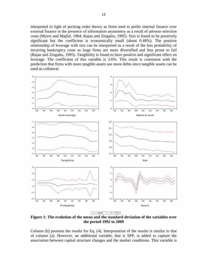
observations for each variable are reported. Moreover, Figure 1 presents the evolution of
1 Part of THOMSON DATASTREAM database
12
the mean of the variables from year to year with the solid line. A one standard deviation
interval is also presented with the dotted lines.
Table 1: Descriptive statistics
Mean Median Maximum Minimum Std. Dev. Observations
LEV_TB 0.251 0.233 0.997 0.000 0.196 7978
MB 1.116 0.918 9.297 0.000 0.737 7978
TANGIBLE 0.403 0.394 0.999 0.000 0.222 7978
SIZE 19.104 19.026 23.969 9.250 1.545 7955
PROFIT 0.067 0.075 11.096 -2.434 0.188 7978
SPP -0.074 -0.048 2.238 -3.258 0.565 7829
Notably, book leverage has peaked between 1997 and 1998 just before or concurrent with
the financial crisis. The leverage ratio continues to decrease since that time. Remarkably
also, the sharp decrease in profitability and SPP (return) during the crisis year, however,
the profitability ratio get better after that.
6. ESTIMATION RESULTS AND DISCUSSION
6.1. Tradeoff versus timing motives
Results of estimation of Eq. (3) and Eq. (4) appear in column (a) and column (b) of Table
2, respectively. For diagnostics, the table report the significance levels for both AR(1)
and AR(2). AR(2) is insignificant thus the absence of second order autocorrelation
required for GMM is satisfied. The validity of instruments is satisfied under the Hansen
test also. Wald test of the joint significance of the estimated coefficients indicates that the
regressors are jointly significant in explaining the dependent variable. The number of
instruments is also reported in Table 2 following the recommendation of Roodman
(2006).
In Column (a), the lagged leverage is found to be the most important determinant of
current leverage. Holding all other regressors constant, about 87.4% change in the mean
of current leverage is resulted from a 100% change in the lagged leverage. This is an
evidence for the high persistence of the leverage variable. The lagged dependent variable
is of special importance in the partial adjustment model. If the firm follows an adjustment
policy, the coefficient of this variable must lie between 0 and 1. The speed of adjustment
equal unity minus this coefficient as will be discussed in Section 6-2.
The growth options as proxied by market-to-book ratio are found to be positively related
to book leverage ratio. The coefficient of this variable is about 1.1%. The positive
relationship is usually interpreted as supporting simple pecking order where funds needed
for growth in excess of retained earnings are obtained using debt. This result is consistent
with the findings of Booth et al. (2001). Profitability has high significant negative effect.
The coefficient of profitability is -21.5% which makes it the second most important firm
characteristic in determining the leverage ratio in the short run next to the lagged
leverage. The negative result is consistent with most empirical works and can be
13
interpreted in light of pecking order theory as firms tend to prefer internal finance over
external finance in the presence of information asymmetry as a result of adverse selection
costs (Myers and Majluf, 1984; Rajan and Zingales, 1995). Size is found to be positively
significant but the coefficient is economically small (about 0.48%). The positive
relationship of leverage with size can be interpreted as a result of the less probability of
incurring bankruptcy costs as large firms are more diversified and less prone to fail
(Rajan and Zingales, 1995). Tangibility is found to have positive and significant effect on
leverage. The coefficient of this variable is 3.6%. This result is consistent with the
prediction that firms with more tangible assets use more debts since tangible assets can be
used as collateral.
Figure 1: The evolution of the mean and the standard deviation of the variables over
the period 1992 to 2009
Column (b) presents the results for Eq. (4). Interpretation of the results is similar to that
of column (a). However, an additional variable, that is SPP, is added to capture the
association between capital structure changes and the market conditions. This variable is
.0
.1
.2
.3
.4
.5
.6
92 94 96 98 00 02 04 06 08
Book leverage
0
1
2
3
4
92 94 96 98 00 02 04 06 08
Market to book
.1
.2
.3
.4
.5
.6
.7
92 94 96 98 00 02 04 06 08
Tangibility
17
18
19
20
21
22
92 94 96 98 00 02 04 06 08
Size
-.4
-.2
.0
.2
.4
.6
92 94 96 98 00 02 04 06 08
Profitability
-3
-2
-1
0
1
2
92 94 96 98 00 02 04 06 08
Mean +/- 1 S.D.
Return
14
found to be negatively and significantly related to leverage as expected. A 10% increase
in SPP is associated with 1.7% decrease in leverage. The SOA for both models is
discussed next.
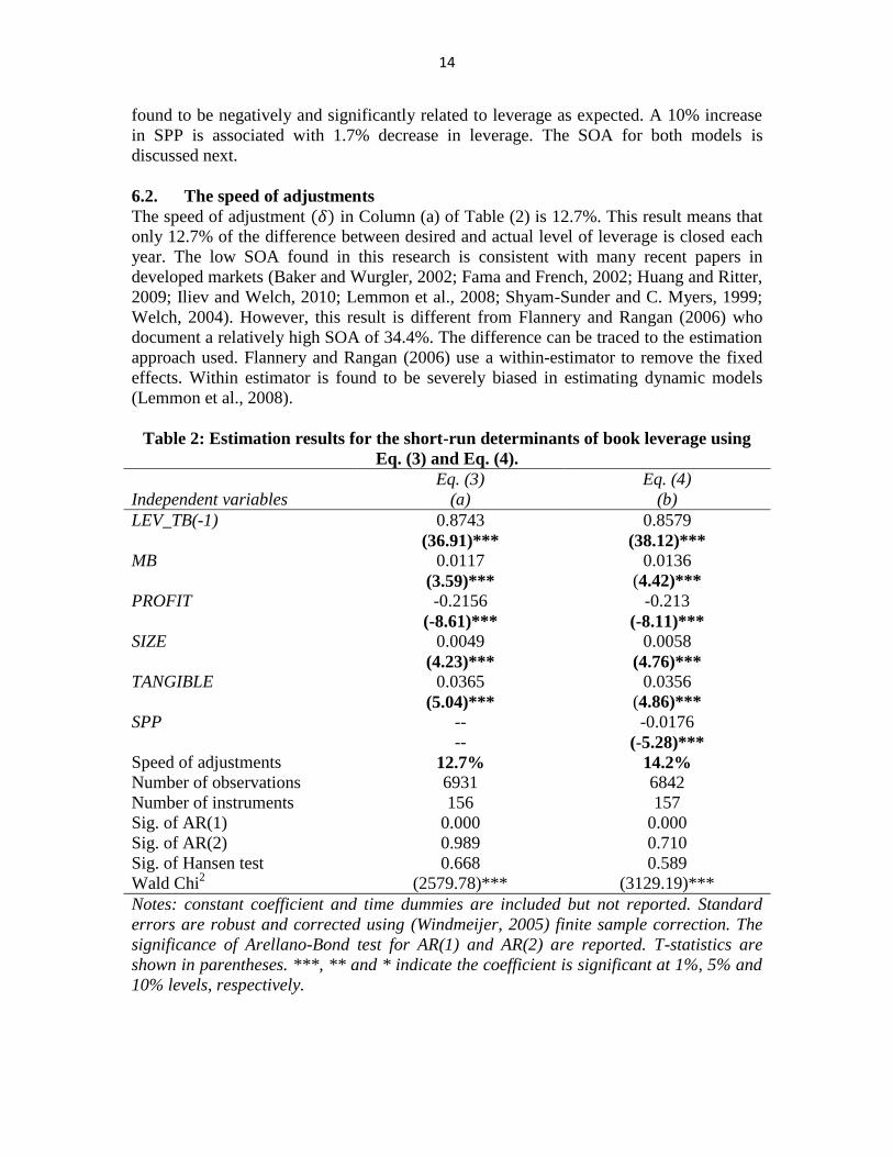
6.2. The speed of adjustments
The speed of adjustment in Column (a) of Table (2) is 12.7%. This result means that
only 12.7% of the difference between desired and actual level of leverage is closed each
year. The low SOA found in this research is consistent with many recent papers in
developed markets (Baker and Wurgler, 2002; Fama and French, 2002; Huang and Ritter,
2009; Iliev and Welch, 2010; Lemmon et al., 2008; Shyam-Sunder and C. Myers, 1999;
Welch, 2004). However, this result is different from Flannery and Rangan (2006) who
document a relatively high SOA of 34.4%. The difference can be traced to the estimation
approach used. Flannery and Rangan (2006) use a within-estimator to remove the fixed
effects. Within estimator is found to be severely biased in estimating dynamic models
(Lemmon et al., 2008).
Table 2: Estimation results for the short-run determinants of book leverage using
Eq. (3) and Eq. (4).
Eq. (3) Eq. (4)
Independent variables (a) (b)
LEV_TB(-1) 0.8743 0.8579
(36.91)*** (38.12)***
MB 0.0117 0.0136
(3.59)*** (4.42)***
PROFIT -0.2156 -0.213
(-8.61)*** (-8.11)***
SIZE 0.0049 0.0058
(4.23)*** (4.76)***
TANGIBLE 0.0365 0.0356
(5.04)*** (4.86)***
SPP -- -0.0176
-- (-5.28)***
Speed of adjustments 12.7% 14.2%
Number of observations 6931 6842
Number of instruments 156 157
Sig. of AR(1) 0.000 0.000
Sig. of AR(2) 0.989 0.710
Sig. of Hansen test 0.668 0.589
Wald Chi2 (2579.78)*** (3129.19)***
Notes: constant coefficient and time dummies are included but not reported. Standard
errors are robust and corrected using (Windmeijer, 2005) finite sample correction. The
significance of Arellano-Bond test for AR(1) and AR(2) are reported. T-statistics are
shown in parentheses. ***, ** and * indicate the coefficient is significant at 1%, 5% and
10% levels, respectively.
15
The slow SOA found in this paper is not conclusive in supporting or rejecting the tradeoff
theory. The adjustment behavior is significant but it is too small to be the first priority of
the firm. Fama and French (2002) find similar slow SOA ranging between 7% and 17%
and they find it difficult to interpret their results in favor of tradeoff theory. Though the
SOA they find is statistically reliable, it is too slow to draw conclusions in favor or
against tradeoff theory. This result implies that the door is open for other interpretations
that do not have targeting as a distinct behavior.
In Column (b), the SOA becomes 14.2% after introducing the timing variable. Based on
the proposition of Flannery and Rangan (2006), if the firm’s first priority is timing, the
SOA should be less once a variable that capture the timing behavior is included in the
regression. On the other hand, if the priority of the firm is to rebalance toward the target,
the SOA should be high and the timing variable should not be able to reduce the targeting
behavior.
The result of adding the timing variable appears to slightly increase, not decrease, the
SOA. This result counters the intuition of Flannery and Rangan (2006). The question
becomes what is the interpretation of the increase in the SOA noticed in Column (b). To
answer this question, recall that the adjustment behavior of the firm is impeded by the
adjustment costs (i.e. the costs of issuing new securities). Adjustment costs are usually
thought of as the reason why the firm does not adjust instantly to any shock to leverage.
The perceived timing is an opportunity for the firm to offset the cost of adjustment by
issuing overvalued shares. Reducing the cost of adjustment of the firm is likely to
encourage the firm to adjust faster. The timing variable seems to capture this reduction in
the cost of adjustment. The overall results are more consistent with the proposition that
both targeting and timing motives are co-existing.
6.3. Controlling for the direction of the deviation from the target
Lastly, this research hypothesize that timing versus targeting behaviors are moderated by
the direction of the deviation from the target. The switch in the preference between the
two motives is a result of the difference in the behavior of the costs and benefits
associated with both tradeoff and timing motives between over and under-leveraged
firms. Costs of being overleveraged are higher and increasing sharply as the firm deviates
more above the target, while costs of being more underleveraged are lower and do not
encounter such sharp increase in costs. Firms that are overleveraged face more pressure
to adjust and less flexibility to time the market as their priority is to get back to the target
whatever the market conditions are. Firms that are underleveraged face relatively lower
pressure to adjust and more flexibility to exploit timing opportunities.
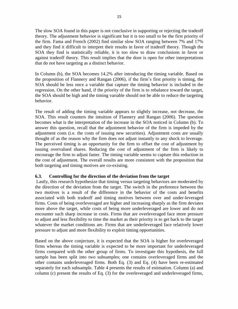
Based on the above conjecture, it is expected that the SOA is higher for overleveraged
firms whereas the timing variable is expected to be more important for underleveraged
firms compared with the other group of firms. To investigate this hypothesis, the full
sample has been split into two subsamples; one contains overleveraged firms and the
other contains underleveraged firms. Both Eq. (3) and Eq. (4) have been re-estimated
separately for each subsample. Table 4 presents the results of estimation. Column (a) and
column (c) present the results of Eq. (3) for the overleveraged and underleveraged firms,
16
respectively. These two columns are presented for comparison purposes. Column (b) and
column (d) present the estimation results of Eq. (4) for the overleveraged and
underleveraged firms, respectively. Adding the timing variable slightly increases the
SOA for overleveraged firms by 1.3% while it increases the SOA for underleveraged
firms by 2.2%. It is likely that timing affects the targeting behavior by reducing the cost
of adjustments more for underleveraged firms. Discussion of the results for each sub-
sample separately is largely similar to the previous discussion of the full sample. More
interesting is the comparison between the two samples. Comparison between column (b)
and column (d) appears in column (e) (see the appendix for computation method of (e)).
Table 4: Estimation results of Eq. (3) and Eq. (4) for both overleveraged and
underleveraged firms
Overleveraged firms Underleveraged firms Difference
(a) (b) (c) (d) (e) =
Eq. (3) Eq. (4) Eq. (3) Eq. (4) (d)-(b)
LEV_TB(-1) 0.706 0.693 0.869 0.847 0.154
(9.41)*** (10.13)*** (21.08)*** (19.66)*** (1.9477)**
[0.075] [0.068] [0.041] [0.043]
MB 0.020 0.022 0.0029 0.004 -0.018
(4.62)*** (5.12)*** (1.09) (1.49) (-3.56)***
[0.004] [0.004] [0.0026] [0.0028]
PROFIT -0.261 -0.278 -0.126 -0.116 -0.162
(-8.04)*** (-8.86)*** (-3.93)*** (-4.27)*** (-3.9)***
[0.032] [0.031] [0.032] [0.027]
SIZE 0.0045 0.0054 0.0026 0.0033 -0.0021
(2.35)** (2.71)*** (2.14)** (2.88)*** (-0.94)
[0.0019] [0.002] [0.0012] [0.0012]
TANGIBLE 0.0477 0.0426 0.015 0.0183 -0.024
(3.26)*** (3.45)*** (2.35)** (2.68)*** (-1.76)**
[0.0146] [0.0123] [0.0064] [0.0069]
SPP -0.010 -0.022 0.012
(-1.84)* (-7.01)*** (1.86)**
[0.0056] [0.0031]
Speed of
adjustments 29.4% 30.7% 13.1% 15.3%
Number of
observations 2384 2357 2644 2614
Number of
instruments 156 157 154 155
AR(1) Sig. + 0.000 0.000 0.000 0.000
AR(2) Sig.+ 0.679 0.724 0.942 0.946
Hansen test 0.352 0.425 0.454 0.408
Wald (888.94)*** (962.86)*** (1169.21)*** (1208.24)***
Notes: constant coefficient and time dummies are included with all models but not
reported. Standard errors in brackets are robust and corrected using Windmeijer (2005)
finite sample correction. The significance level of Arellano-Bond test for AR(1) and
17
AR(2) are reported. T-statistics are shown in parentheses. ***, ** and * indicate the
coefficient is significant at 1%, 5% and 10% levels, respectively.
In general, firms are found to be much more sensitive to be overleveraged than to be
underleveraged. The SOA for overleveraged firms is much higher (about 30.7%) than
underleveraged firms (15.3%). The timing coefficient for underleveraged firms is more
than doubled than that of overleveraged firms. For overleveraged firms the coefficient of
timing is 1% and it is significant only at p=10% level while for underleveraged firms the
coefficient is 2.2% and it is significant at p=1% level. It is apparent that underleveraged
firms are more affected by market valuation and less hurry to adjust to the target.
The higher coefficient of SPP for underleveraged firms is not likely to be a result of
growth options. The variable that is supposed to capture growth, market-to-book ratio, is
actually much higher for overleveraged firms than for underleveraged firms in which it is
insignificant. Profitability may signal growth but it is higher for overleveraged firms also.
The tangibility variable is higher for overleveraged firms as it is more important to reduce
the costs of distress for these firms (Harris and Raviv, 1990). All the variables that are
thought to relate with the tradeoff dynamism are higher for the overleveraged firms. SPP
is the only factor that is higher for underleveraged firms.
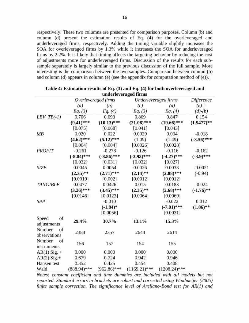
6.4. New insight to the role of historical timing of Baker and Wurgler (2002) as a
capital structure determinant
In their seminal paper, (Baker and Wurgler, 2002) propose a timing variable that captures
the history of timing activities of the firm and they called it the temporal “external
finance weighted-average market-to-book” ratio (EFWAMB). For a given firm-year, this
variable is defined as
Eq. (5)
where e and d denote net equity and net debt issues, respectively. The sum of e+d is the
external financing raised each year.
is market-to-book ratio. The weight for
each year is the ratio of external financing raised by the firm in that year to the total
external financing raised by the firm in years (0) through (t-1). Negative weights are reset
to zero. This variable takes high values for firms that raise external finance when the MB
ratio is high and low values for firms that raise external finance while the MB ratio is
low. This paper defines (e) as while (d) is
defined as .
Abdeljawad and Mat Nor (2011) find that this variable is significant in determining the
capital structure for Malaysian firms. If firms time the mispricing periods and they do not
rebalance the effect of this timing, timing effect may accumulate over time and hence the
history of timing will continue affecting the current leverage. If the hypothesis about the
asymmetric effect of timing is valid in the short run, it should continue to hold in the long
run. To investigate this possibility, this research will re-run a model similar to that used
by (Abdeljawad and Mat Nor, 2011; Baker and Wurgler, 2002) but with a dummy
variable that captures whether the firm is overleveraged or underleveraged and an
18
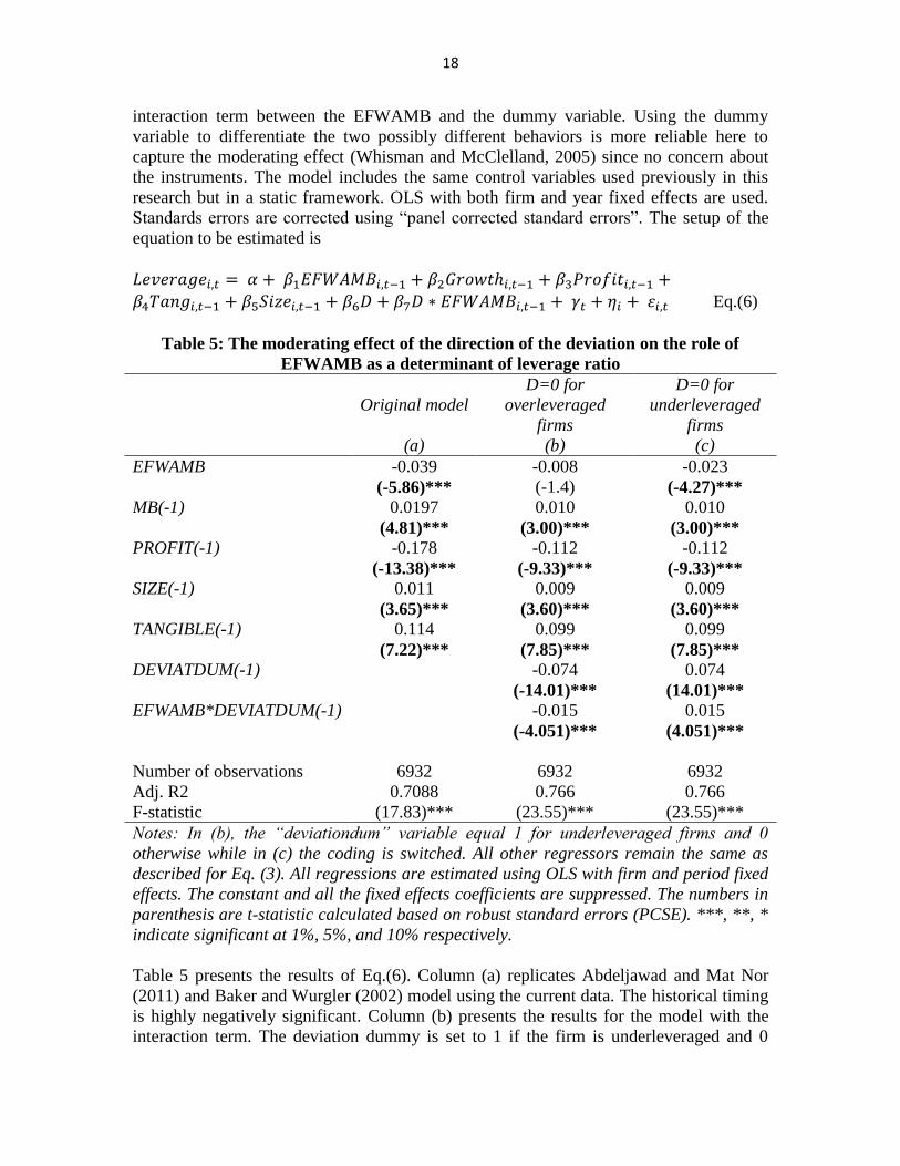
interaction term between the EFWAMB and the dummy variable. Using the dummy
variable to differentiate the two possibly different behaviors is more reliable here to
capture the moderating effect (Whisman and McClelland, 2005) since no concern about
the instruments. The model includes the same control variables used previously in this
research but in a static framework. OLS with both firm and year fixed effects are used.
Standards errors are corrected using “panel corrected standard errors”. The setup of the
equation to be estimated is
Eq.(6)
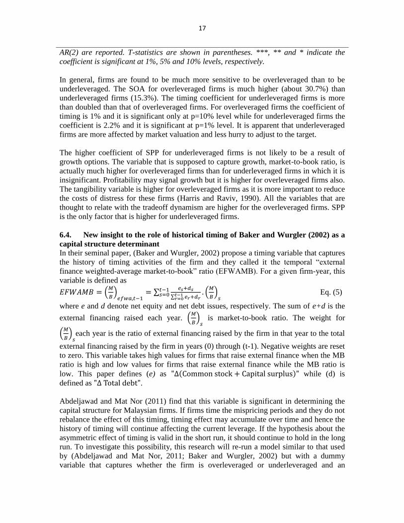
Table 5: The moderating effect of the direction of the deviation on the role of
EFWAMB as a determinant of leverage ratio
Original model
D=0 for
overleveraged
firms
D=0 for
underleveraged
firms
(a) (b) (c)
EFWAMB -0.039 -0.008 -0.023
(-5.86)*** (-1.4) (-4.27)***
MB(-1) 0.0197 0.010 0.010
(4.81)*** (3.00)*** (3.00)***
PROFIT(-1) -0.178 -0.112 -0.112
(-13.38)*** (-9.33)*** (-9.33)***
SIZE(-1) 0.011 0.009 0.009
(3.65)*** (3.60)*** (3.60)***
TANGIBLE(-1) 0.114 0.099 0.099
(7.22)*** (7.85)*** (7.85)***
DEVIATDUM(-1) -0.074 0.074
(-14.01)*** (14.01)***
EFWAMB*DEVIATDUM(-1) -0.015 0.015
(-4.051)*** (4.051)***
Number of observations 6932 6932 6932
Adj. R2 0.7088 0.766 0.766
F-statistic (17.83)*** (23.55)*** (23.55)***
Notes: In (b), the “deviationdum” variable equal 1 for underleveraged firms and 0
otherwise while in (c) the coding is switched. All other regressors remain the same as
described for Eq. (3). All regressions are estimated using OLS with firm and period fixed
effects. The constant and all the fixed effects coefficients are suppressed. The numbers in
parenthesis are t-statistic calculated based on robust standard errors (PCSE). ***, **, *
indicate significant at 1%, 5%, and 10% respectively.
Table 5 presents the results of Eq.(6). Column (a) replicates Abdeljawad and Mat Nor
(2011) and Baker and Wurgler (2002) model using the current data. The historical timing
is highly negatively significant. Column (b) presents the results for the model with the
interaction term. The deviation dummy is set to 1 if the firm is underleveraged and 0
19
otherwise. The interaction term is significant indicating that the direction of the deviation
from the target is able to moderate the relationship between EFWAMB and leverage. A
simple way to find the direct effect of EFWAMB in each subsample is to switch the
coding of the dummy variable and noting the coefficient of EFWAMB (Whisman and
McClelland, 2005). The direct effect of EFWAMB when firms are overleveraged is not
significant in column (b) while it is highly significant for the underleveraged firms as
appear in column (c). It can be concluded that underleveraged firms are more inclined to
exploit mispricing opportunities and the effect of this timing behavior takes longer time
to be rebalanced. This result may add doubt to the generalizability of the timing theory
since the results of Baker and Wurgler (2002) may be driven by underleveraged firms as
the period of their study, the late 1980’s and the 1990’s, are characterized by the low
leverage used by firms (Huang and Ritter, 2009).
7. CONCLUSIONS
Using an estimator that is found to be more efficient for estimating dynamic panel data
with short time dimension, that is system GMM; this study reveals that Malaysian firms
are adjusting their capital structure to the target but at a slow rate. At the same time, firms
consider timing of the market conditions as an important factor when making financial
decisions. This study finds evidence for asymmetric timing behavior as well as targeting
behavior between firms over- and underleveraged. Specifically, overleveraged firms
adjust to the target faster and they are less concern with timing. On the other side,
underleveraged firms adjust slower but they consider timing more seriously. This
behavior is likely to result from taking into account all the costs and benefits of being at
the target, adjustment toward the target and timing opportunities. Deviating from the
target to the upper side is likely to be more costly than deviating below the target because
bankruptcy costs and agency costs of debt will intensify quickly as the firm deviates more
above the target. Hence, overleveraged firms need to adjust faster to reduce these costs
despite the market conditions. Underleveraged firms are less urged to adjust and hence it
is feasible for them to consider market conditions more in their financing decisions.
These results are confirmed in the short run as well as long run modeling.
The finding of this study supports that firms consider both targeting and timing in their
financing decisions. No standalone theory can interpret the full spectrum of empirical
results. This result is consistent with the view of Myers (2003) that capital structure
“theories are conditional not general”.
REFERENCES Abdeljawad, I., Mat Nor, F., 2011. Equity Market Timing and Capital Structure: Evidence from
Malaysia., 13th Malaysian Finance Association, Langkawi, Malaysia. Alti, A., 2006. How Persistent Is the Impact of Market Timing on Capital Structure? The Journal
of Finance 61, 1681-1710. Antoniou, A., Guney, Y., Paudyal, K., 2008. The determinants of capital structure: capital market-
oriented versus bank-oriented institutions. Journal of Financial and Quantitative analysis 43, 59-92.
20
Arellano, M., Bond, S., 1991. Some tests of specification for panel data: Monte Carlo evidence and an application to employment equations. The Review of Economic Studies 58, 277.
Arellano, M., Bover, O., 1995. Another look at the instrumental variable estimation of error-components models* 1. Journal of econometrics 68, 29-51.
Baker, M., Wurgler, J., 2002. Market Timing and Capital Structure. The Journal of Finance 57, 1-32.
Baxter, N.D., 1967. Leverage, risk of ruin and the cost of capital. Journal of Finance 22, 395-403. Blundell, R., Bond, S., 1998. Initial conditions and moment restrictions in dynamic panel data
models. Journal of econometrics 87, 115-143. Bolger, F. & Harvey, N. 1993. Context-Sensitive Heuristics in Statistical Reasoning. The
Quarterly Journal of Experimental Psychology Section A 46(4): 779-811. Booth, L., Aivazian, V., Demirguc-Kunt, A., Maksimovic, V., 2001. Capital structures in developing
countries. Journal of Finance 56, 87-130. Bradley, M., Jarrell, G.A., Kim, E.H., 1984. On the Existence of an Optimal Capital Structure:
Theory and Evidence. The Journal of Finance 39, 857-878. Byoun, S., 2008. How and When Do Firms Adjust Their Capital Structures toward Targets? The
Journal of Finance 63, 3069-3096. Clark, B.J., Francis, B.B., Hasan, I., 2009. Do Firms Adjust Toward Target Capital Structures? Some
International Evidence. SSRN eLibrary. Clogg, C.C., Petkova, E., Haritou, A., 1995. Statistical Methods for Comparing Regression
Coefficients Between Models. American Journal of Sociology 100, 1261-1293. Cohen, A., 1983. Comparing Regression Coefficients Across Subsamples. Sociological Methods &
Research 12, 77-94. Cook, D.O., Tang, T., 2010. Macroeconomic conditions and capital structure adjustment speed.
Journal of Corporate Finance 16, 73-87. De Bie, T., De Haan, L., 2007. Market timing and capital structure: Evidence for Dutch firms.
Economist 155, 183-206. Deangelo, H. & Masulis, R. W. 1980. Optimal Capital Structure under Corporate and Personal
Taxation. Journal of Financial Economics 8(1): 3-29.
de Miguel, A., Pindado, J., 2001. Determinants of capital structure: new evidence from Spanish panel data. Journal of Corporate Finance 7, 77-99.
Deesomsak, R., Paudyal, K., Pescetto, G., 2004. The determinants of capital structure: evidence from the Asia Pacific region. Journal of Multinational Financial Management 14, 387-405.
Drobetz, W., Wanzenried, G., 2006. What determines the speed of adjustment to the target capital structure? Applied Financial Economics 16, 941-958.
Fama, E.F., French, K.R., 2002. Testing Trade-Off and Pecking Order Predictions about Dividends and Debt. The Review of Financial Studies 15, 1-33.
Flannery, M.J., Hankins, K.W., 2007. A theory of capital structure adjustment speed. Unpublished Manuscript, University of Florida.
Flannery, M.J., Rangan, K.P., 2006. Partial adjustment toward target capital structures. Journal of Financial Economics 79, 469-506.
Frank, M.Z., Goyal, V.K., 2007. Trade-Off and Pecking Order Theories of Debt. SSRN eLibrary. Graham, J.R., Harvey, C.R., 2001. The theory and practice of corporate finance: evidence from
the field. Journal of Financial Economics 60, 187-243. Harris, M., Raviv, A., 1990. Capital structure and the informational role of debt. Journal of
Finance 45, 321-349.
21
Homaifar, G., Zietz, J., Benkato, O., 1994. An empirical model of capital structure: some new evidence. Journal of Business Finance & Accounting 21, 1-14.
Hovakimian, A., 2006. Are observed capital structures determined by equity market timing? Journal of Financial and Quantitative analysis 41, 221-243.
Hovakimian, A., Li, G., 2011. In search of conclusive evidence: How to test for adjustment to target capital structure. Journal of Corporate Finance 17, 33-44.
Hovakimian, A., Opler, T., Titman, S., 2001. The Debt-Equity Choice. The Journal of Financial and Quantitative Analysis 36, 1-24.
Huang, R., Ritter, J., 2009. Testing theories of capital structure and estimating the speed of adjustment. Journal of Financial and Quantitative analysis 44, 237-271.
Hussain, M.I., 2005. Determenation of capital structure and prediction of corporate financial distress. Univirsity Putra Malaysia.
Iliev, P., Welch, I., 2010. Reconciling estimates of the speed of adjustment of leverage ratios. SSRN eLibrary.
Jensen, M., 1986. Agency costs of free cash flow, corporate finance, and takeovers. The American Economic Review 76, 323-329.
Jensen, M., Meckling, W., 1976. Theory of the firm: Managerial behavior, agency costs and ownership structure. Journal of Financial Economics 3, 305-360.
Kayhan, A., Titman, S., 2007. Firms' histories and their capital structures. Journal of Financial Economics 83, 1-32.
Kraus, A. & Litzenberger, R. 1973. A State-Preference Model of Optimal Financial Leverage.
Journal of Finance 28(4): 911-922.
Leary, M.T., Roberts, M.R., 2005. Do Firms Rebalance Their Capital Structures? The Journal of Finance 60, 2575-2619.
Lemmon, M.L., Roberts, M.R., Zender, J.F., 2008. Back to the Beginning: Persistence and the Cross Section of Corporate Capital Structure. The Journal of Finance 63, 1575-1608.
Mahajan, A., Tartaroglu, S., 2008. Equity market timing and capital structure: International evidence. Journal of Banking & Finance 32, 754-766.
Myers, S., 1977. Determinants of corporate borrowing. Journal of Financial Economics 5, 147-175.
Myers, S., Majluf, N., 1984. Corporate financing and investment decisions when firms have informationthat investors do not have. Journal of Financial Economics 13, 187-221.
Myers, S.C., 1984. The Capital Structure Puzzle. The Journal of Finance 39, 575-592. Myers, S.C., 2003. Chapter 4 Financing of corporations, in: G.M. Constantinides, M.H., Stulz,
R.M. (Eds.), Handbook of the Economics of Finance. Elsevier, pp. 215-253. Ozkan, A., 2001. Determinants of Capital Structure and Adjustment to Long Run Target:
Evidence From UK Company Panel Data. Journal of Business Finance & Accounting 28, 175-198.
Paternoster, R., Brame, R., Mazerolle, P., Piquero, A., 1998. Using the correct statistical test for the equality of regression coefficients. Criminology 36, 859-866.
Rajan, R., Zingales, L., 1995. What do we know about capital structure? Some evidence from international data. Journal of Finance 50, 1421-1460.
Roodman, D., 2006. How to do xtabond2: An Introduction to" Difference" and" System" GMM in Stata. Center for global development.
Shyam-Sunder, L., C. Myers, S., 1999. Testing static tradeoff against pecking order models of capital structure. Journal of Financial Economics 51, 219-244.
Smith, D.J., Chen, J., Anderson, H.D., 2010. Partial Adjustment Towards Target Capital Structure: Evidence from New Zealand. SSRN eLibrary.
22
Strebulaev, I. & Yang, B. 2007. The Mystery of Zero-Leverage Firms. working paper,
Stanford University.
Titman, S., Wessels, R., 1988. The Determinants of Capital Structure Choice. The Journal of Finance 43, 1-19.
Tversky, A. & Kahneman, D. 1974. Judgment under Uncertainty: Heuristics and Biases. science 185(4157): 1124-1131.
Welch, I., 2004. Capital Structure and Stock Returns. The Journal of Political Economy 112, 106-131.
Whisman, M.A., McClelland, G.H., 2005. Designing, testing, and interpreting interactions and moderator effects in family research. Journal of Family Psychology 19, 111.
Windmeijer, F., 2005. A finite sample correction for the variance of linear efficient two-step GMM estimators. Journal of econometrics 126, 25-51.
APPENDICES
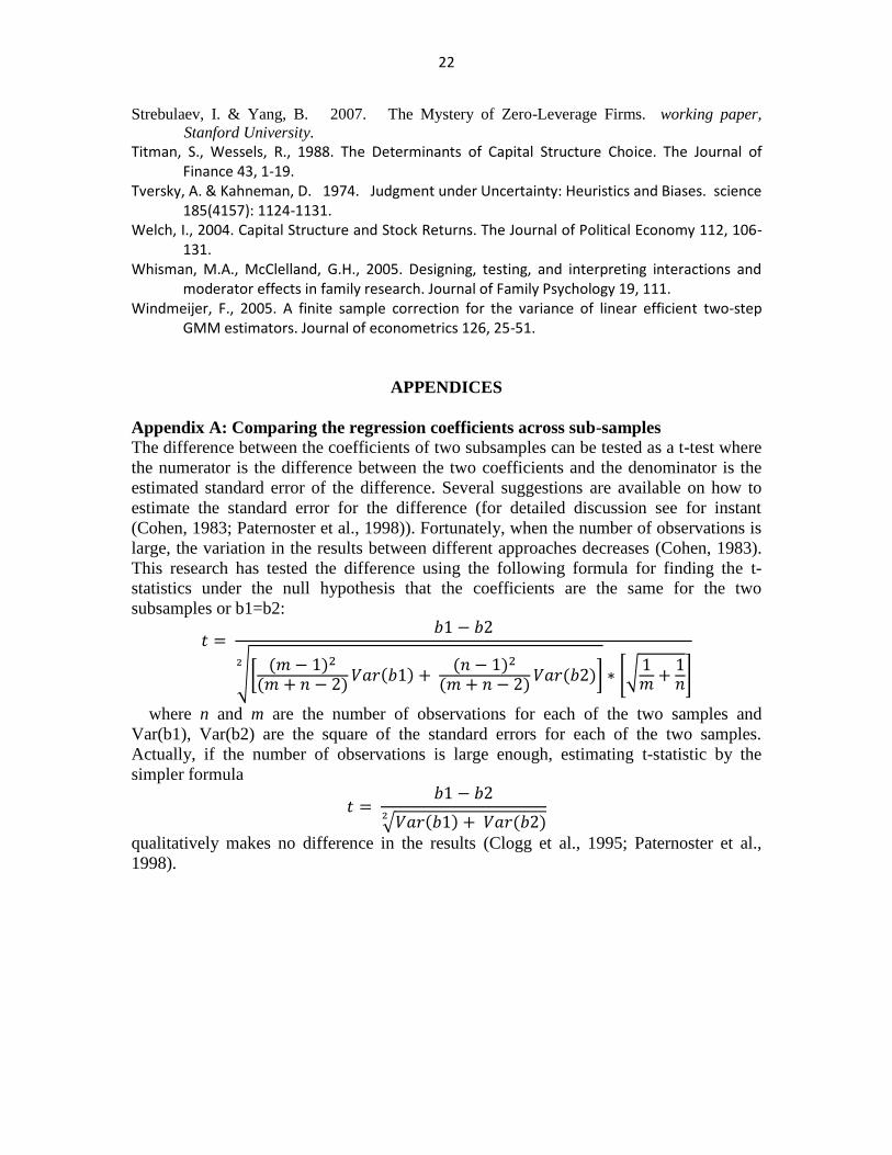
Appendix A: Comparing the regression coefficients across sub-samples
The difference between the coefficients of two subsamples can be tested as a t-test where
the numerator is the difference between the two coefficients and the denominator is the
estimated standard error of the difference. Several suggestions are available on how to
estimate the standard error for the difference (for detailed discussion see for instant
(Cohen, 1983; Paternoster et al., 1998)). Fortunately, when the number of observations is
large, the variation in the results between different approaches decreases (Cohen, 1983).
This research has tested the difference using the following formula for finding the t-
statistics under the null hypothesis that the coefficients are the same for the two
subsamples or b1=b2:
where n and m are the number of observations for each of the two samples and
Var(b1), Var(b2) are the square of the standard errors for each of the two samples.
Actually, if the number of observations is large enough, estimating t-statistic by the
simpler formula
qualitatively makes no difference in the results (Clogg et al., 1995; Paternoster et al.,
1998).