Accounting for the Timing of Costs and Benefits in the Evaluation of Health Projects Relevant to LMICs    

Karl Claxton 

 

  

 

March 2018 

 

 

 

Guidelines for Benefit‐Cost Analysis Project 

Working Paper No. 8 

 

 

 

Prepared for the Benefit‐Cost Analysis Reference Case Guidance Project 

Funded by the Bill and Melinda Gates Foundation 

 

  

Visit us on the web: https://sites.sph.harvard.edu/bcaguidelines/ 

   

2  

Accounting for the timing of costs and benefits in the evaluation of health 

projects relevant to LMICs  

 

Karl Claxton 

 

 

 

 

 

 

I would like to acknowledge and thank the participants of the BMGF funded workshop on discounting 

on 14th September 2017 for their insightful presentations and discussion of topics that have informed 

this paper.  I would also like to acknowledge  and thanks the following people who kindly provided 

very useful comments on an earlier draft of this paper: Miqdad Asaria, Fiammetta Bozzani, Werner 

Brouwer, Maria Petro Brunal, Collins Chansa, Maureen Cropper, Tom Drake, Mark Freeman, Ben 

Groom, Markus Haacker, Julian Jamison, Mark Jit, Paul Kelleher, Margaret Kuklinski, Carol Levin, 

James Lomas, Jessica Ochalek, Mike Paulden, Catherine Pitt, Billy Pizer, Michelle Remme, Zia Sadique, 

Michael Spackman, Sedona Sweeney, Fran Sussman, Gernot Wagner and David Wilson. Any errors, 

omissions and misrepresentations are the responsibility of the author  

  

 

 

 

 

 

 

 

 

 

 

 

 

 

3  

Executive summary 

The primary focus of this paper is to offer guidance on the analysis of time streams of multiple 

effects that a project may have (e.g., on health, health care costs and consumption) so that they can 

then be discounted appropriately.  This requires a framework within which CEA and CBA can be 

understood and that identifies the common parameters that need to be assessed.   

The common conceptual framework for CEA and BCA, which is set out in Section 2, identifies the key 

parameters required to express the time streams of multiple effects in a common numeraire of 

equivalent consumption gains and losses which can then be discounted at a social time preference 

rate for consumption.  

Extensive reporting is recommended, as illustrated in Tables 1, 2a and 2b.  Reporting the results of 

CEA and BCA in this way makes the assessments required explicit so the impact of alternative 

assumptions can be explored and analysis updated as better estimates evolve.  

The quantification and conversion of the time streams of multiple effects into their equivalent 

health, health care cost or consumption effects avoids embedding multiple augments in discounting 

policies. This helps to identify where parameters are likely to differ in particular contexts, what type 

of evidence would be relevant, what is currently known that is relevant to low and middle income 

settings and how this evidence might be strengthened. 

The separate and explicit accounting for these arguments provides clarity about the parameters that 

need to be assessed and so they can be applied consistently, while preserving the possibility of 

accountable deliberation about evidence, values and unquantified arguments in decision making 

processes.   

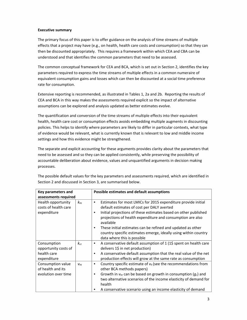
The possible default values for the key parameters and assessments required, which are identified in 

Section 2 and discussed in Section 3, are summarised below.   

Key parameters and assessments required 

Possible estimates and default assumptions 

Health opportunity costs of health care expenditure 

kht  

• Estimates for most LMICs for 2015 expenditure provide initial default estimates of cost per DALY averted 

• Initial projections of these estimates based on other published projections of health expenditure and consumption are also available    

• These initial estimates can be refined and updated as other country specific estimates emerge, ideally using within country data where this is possible 

Consumption opportunity costs of health care expenditure 

kct  

• A conservative default assumption of 1 (1$ spent on health care delivers 1$ in net production) 

• A conservative default assumption that the real value of the net production effects will grow at the same rate as consumption 

Consumption value of health and its evolution over time 

 

vht  

• Country specific estimate of vh (see the recommendations from other BCA methods papers) 

• Growth in vht can be based on growth in consumption (gc) and two alternative scenarios of the income elasticity of demand for health   

• A conservative scenario using an income elasticity of demand 

4  

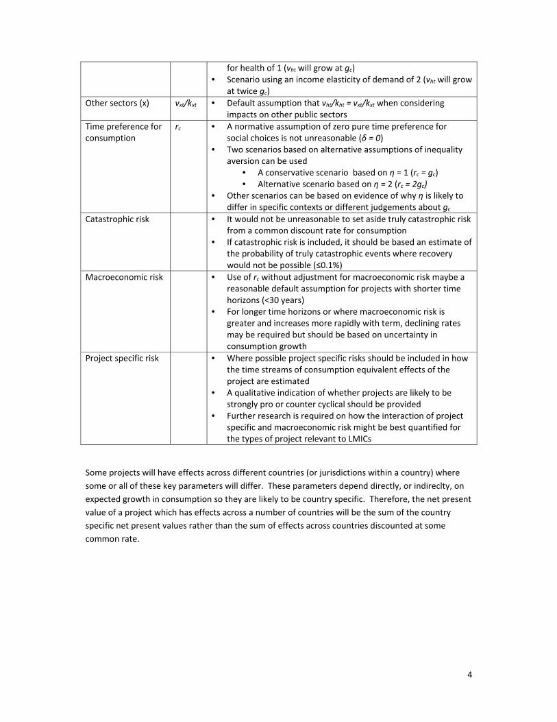
for health of 1 (vht will grow at gc)• Scenario using an income elasticity of demand of 2 (vht will grow 

at twice gc) 

Other sectors (x)   

vxt/kxt  

• Default assumption that vht/kht = vxt/kxt when considering impacts on other public sectors 

Time preference for consumption  

rc  

• A normative assumption of zero pure time preference for  social choices is not unreasonable (δ = 0) 

• Two scenarios based on alternative assumptions of inequality aversion can be used 

• A conservative scenario  based on η = 1 (rc = gc) • Alternative scenario based on η = 2 (rc = 2gc) 

• Other scenarios can be based on evidence of why η is likely to differ in specific contexts or different judgements about gc   

Catastrophic risk  

  • It would not be unreasonable to set aside truly catastrophic risk from a common discount rate for consumption 

• If catastrophic risk is included, it should be based an estimate of the probability of truly catastrophic events where recovery would not be possible (≤0.1%) 

Macroeconomic risk  

  • Use of rc without adjustment for macroeconomic risk maybe a reasonable default assumption for projects with shorter time horizons (<30 years) 

• For longer time horizons or where macroeconomic risk is greater and increases more rapidly with term, declining rates may be required but should be based on uncertainty in consumption growth 

Project specific risk    • Where possible project specific risks should be included in how the time streams of consumption equivalent effects of the project are estimated 

• A qualitative indication of whether projects are likely to be strongly pro or counter cyclical should be provided 

• Further research is required on how the interaction of project specific and macroeconomic risk might be best quantified for the types of project relevant to LMICs 

 

Some projects will have effects across different countries (or jurisdictions within a country) where 

some or all of these key parameters will differ.  These parameters depend directly, or indireclty, on 

expected growth in consumption so they are likely to be country specific.  Therefore, the net present 

value of a project which has effects across a number of countries will be the sum of the country 

specific net present values rather than the sum of effects across countries discounted at some 

common rate.   

 

 

 

 

 

5  

Contents                                            Page 

Executive Summary                2  

1  Introduction                  5                    2  Conceptual framework                6              

2.1  The objective of the project is to improve health       6 

2.1.1   Why discount health?            6 

2.1.2   Representing the effects of health care projects      7 

2.1.3   Non‐health impacts and non‐health care costs      10 

2.2   The objective of the project is to improve welfare      12 

2.3  What is the distinction between CEA and BCA?        13 

 

3  Evidence available to inform key parameters and possible default estimates  14 

     

3.1  Health opportunity costs of health care expenditure       14 

  3.2  Consumption opportunity costs of health care expenditure    15 

3.3  Consumption value of health and its evolution over time     16 

  3.4  Other constrained sectors            17 

3.5  Time preference for consumption          18 

3.6  Catastrophic, macroeconomic and project specific risk      19 

       

4  Recommendations, reporting and further research        22 

   

4.1  A summary possible default estimates          22 

4.2  Reporting and aggregating effects          23 

  4.3  Suggestions for further research           24 

 

 

 

 

 

 

 

 

 

 

 

 

 

6  

1.  Introduction 

A decision to introduce a policy (e.g., public health, educational, environmental etc.) or provide an 

effective intervention (e.g., a health technology or programme of care for a particular indication) for 

the current population may offer some immediate health benefits but, in many circumstances, the 

health benefits will occur in future periods. Other projects are intended to reduce the risk of future 

events for the current population and others may also reduce risks for future incident patients, so 

the health benefits they offer will not be fully realized for many years. Future benefits are not 

restricted to health but may also include impacts on private consumption, reductions in future 

health care costs and other forms of public expenditure as well as social objectives of particular 

interest to the decision maker.  Similarly, different policy choices and projects will not just impose 

health care and other costs in the current period but in future periods as well. 

 

The question is how account should be taken of when health care and other costs are incurred and 

health and other benefits are received.  The intention is to offer clarity about principles, the key 

assessment required and the evidence currently available to inform them, so that decision makers in 

low and middle income countries (LMICs) and other stakeholders, are better placed to judge what 

would be an appropriate analysis of the time streams of the multiple effects that a project may have 

and the discount policy to apply to them in a particular context. This includes how global bodies, 

which make recommendations (e.g., WHO), purchase health technologies (e.g., Global Fund) or 

prioritise the development of new ones (e.g., BMGF), should judge the value of projects which have 

effects in many different settings where appropriate discounting of costs and benefits are likely to 

differ.   

 

The primary focus of this paper is to offer guidance on the appropriate analysis of time streams of 

multiple effects that a project may have (e.g., on health, health care costs and consumption) so that 

they can then be discounted appropriately.  This requires framework within which cost‐effectiveness 

analysis (CEA) and benefit–cost analysis (BCA) can be understood that identifies the common key 

parameters that need to be assessed.  This also helps to identify where parameters are likely to 

differ in particular contexts, what type of evidence would be relevant, what is currently known that 

is relevant to low and middle income settings and how this evidence might be strengthened. 

 

An explicit assessment of the opportunity costs associated with current constraints and the relative 

value of multiple effects shows that the distinction between a CEA which accounts for wider effects 

and a BCA, which incorporates the opportunity of cost or shadow prices of existing constraints, is 

more apparent than real.     Both require the same assessment of the same key parameters.   

Reporting the results of CEA and BCA in an extensive way means that discounting procedures do not 

embed multiple arguments, but expose the assessment required. This also enables the impact of 

alternative, but plausible, scenarios to be explored and analysis to be updated as better estimates 

evolve.   The quantification and conversion of the time streams of multiple effects into their 

equivalent health, health care cost or consumption effects avoids embedding multiple augments in 

discounting policies. The separate and explicit accounting for these arguments provides clarity about 

the parameters that need to be assessed so they can be applied transparently and consistently, 

while preserving the possibility of accountable deliberation about evidence, values and unquantified 

arguments in decision making processes. 

7  

A common conceptual framework of how times streams of effects on health, health care costs and 

consumption is set out in Section 2.  This identifies the key parameters that need to be assessed 

whether conducting BCA or CEA.  The evidence currently available that might support their 

assessment in LMIC setting is discussed in Section 3 and possible default values are suggested.     

These recommended defaults are summarised in Section 4 before suggesting how analysis might be 

most usefully reported, especially when a project has effects across different contexts where 

parameters are likely to differ. Finally, some suggestions of priorities for further research are made.  

 

 

2  Conceptual framework 

A common conceptual framework within which CEA and CBA can be understood and key parameters 

identified is initially set out for a project which only has effects on time streams of health and health 

care costs. This is extended to consider effects beyond health and health care costs, where the often 

complex reality of multiple sectors is initially simplified into two (collective health care expenditure 

and private consumption) to illustrate principles. The common parameters that need to be assessed 

are identified and the distinction between BCA and CEA is discussed.  A key implication is that 

discounting policies should not embed multiple augments but the quantification and conversion of 

the time streams of multiple effects into their equivalent health, health care cost or consumption 

effects should be done explicitly before they are discounted at a rate appropriate to health, health 

care costs or consumption respectively. 

 

2.1  The objective of the project is to improve health 

Decision making bodies and institutions can be viewed as the agents of a principal (e.g., a socially 

legitimate process such as government) which allocates resources, devolves powers and gives 

responsibility to pursue specific, measurable and therefore narrowly defined objectives, e.g., to 

improve health. The values implied by the outcome of this process (e.g., government implicitly or 

explicitly determining collective expenditure on health care) can be regarded as a partial but 

revealed expression of some unknown social welfare function that may include many conflicting 

arguments, e.g., health equity, social solidarity among many others that are difficult to specify let 

alone quantify (Drummond et al 2015).  In these circumstances economic analysis cannot be used to 

make claims about social welfare or the optimality of the resources allocated to health care. Its role 

is more modest, claiming to inform accountable decision‐making by revealing implied values and 

exposing the implications of current levels of health and other public expenditure.  It is this role that 

economic analysis has tended to play in health policy and underpins much of the evaluation of 

health care projects and CEAs that have been conducted (Drummond et al 2015, Coast et al 2008).1  

2.1.1  Why discount health? 

In this context the reason to discount future health effects cannot appeal to the type of welfare 

arguments that underpin social time preference (STP) for consumption, but instead to the 

opportunity costs of financing health care.  The health care costs of a project could have been 

invested elsewhere in the economy or used to reduce public borrowing at a real rate of return, 

which would provide more health care resources in the future and generate greater health benefits. 

                                                            1 See Drummond et al 2015 Section 2.4.3 pages 33‐38 

8  

Health care transforms resources into health so from the perspective of a social planner trading 

health care resources over time is to trade health. Therefore, if health care costs are discounted to 

reflect the opportunity cost of financing health care, their health effects must also be discounted.2  

For example, real yields on government bonds reflect the marginal cost of increasing health care 

expenditure available to government (Paulden and Claxton 2012; Paulden et al. 2016). In this 

context the broader question of the social opportunity costs of public expenditure including the 

macroeconomic choice of levels and mix of taxation and borrowing (Spackman 2017) can be 

regarded as the responsibility of government rather than spending departments or national and 

supra national decision making and advisory bodies.3 

2.1.2   Representing the effects projects 

Estimates of the additional health care costs (Δch) and additional health effects (Δh) (whether 

measured as Quality Adjusted Life Years, QALYs, gained or Disability Adjusted Life Years Averted, 

DALYs) of a project or a health care intervention are commonly reported as incremental cost‐

effectiveness ratios (ICER).4 These provide a useful summary of how much additional resource is 

required to achieve a measured improvement in health (the additional cost per QALY gained or DALY 

averted). Whether the intervention will improve health outcomes overall requires a comparison with 

a ‘threshold’  (kh) that reflects the likely health opportunity costs, i.e. the improvement in health that 

would have been possible if the additional resources required had, instead, been made available for 

other health care activities.  A project will improve health overall if the additional health benefits 

exceed the health opportunity costs associated with the additional health care costs  that must be 

found from existing commitments, or that require additional expenditure that could have been 

devoted to other health care activities (∆h > ∆ch/kh).5  

Time stream of net health effects 

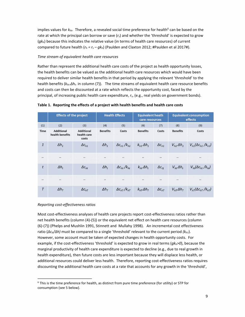
Most projects offer time streams of health effects (Δht) and health care costs (∆cht) illustrated in 

Table 1.  The additional health care costs in each period can be reported as the health opportunity 

costs (∆cht/kht, in column (5) of Table 1)  by applying a ‘threshold’ that reflects an assessment of the 

marginal productivity of health care expenditure relevant to that period (kht).  The time streams of 

health benefits and health opportunity losses can then be discounted at a rate which reflects a social 

time preference for health (rh).   

The social choice of how much resource to devote to health care over time and the resulting health 

in each period reveals something about society’s willingness to trade current and future health.  For 

example, the choice of the principal in setting the level of health expenditure in each period, based 

on expectations about how the marginal productivity of health care expenditure is likely to evolve, 

                                                            2 This is commonly illustrated by a comparison of terminal and present values. The cost per QALY of a project with immediate costs and additional health benefits all occurring at a future point in time is the same whether costs are expressed at their terminal value when the health benefits occur, or discounting the health benefits back to their present value at the same rate (Nord 2011). 3 See Drummond et al 2015, page 108‐112 4 See Drummond et al 2015, Section 2.4.1 page 27‐31 and Section 4.2.1 page 79‐83 5 This is equivalent to asking whether cost per QALY it offers is less than the cost‐effectiveness ‘threshold’ (∆ch/∆h < kh), so long as the ‘threshold’ used to judge cost‐effectives reflect the likely health opportunity costs. 

9  

implies values for kht.  Therefore, a revealed social time preference for health6 can be based on the 

rate at which the principal can borrow or save (rs) and whether the ‘threshold’ is expected to grow 

(gkh) because this indicates the relative value (in terms of health care resources) of current 

compared to future health (rh = rs – gkh) (Paulden and Claxton 2012; #Paulden et al 2017#). 

Time stream of equivalent health care resources 

Rather than represent the additional health care costs of the project as health opportunity losses, 

the health benefits can be valued as the additional health care resources which would have been 

required to deliver similar health benefits in that period by applying the relevant ‘threshold’ to the 

health benefits (kht.∆ht. in column (7)).   The time streams of equivalent health care resource benefits 

and costs can then be discounted at a rate which reflects the opportunity cost, faced by the 

principal, of increasing public health care expenditure, rs, (e.g., real yields on government bonds). 

Table 1.  Reporting the effects of a project with health benefits and health care costs 

 

Reporting cost‐effectiveness ratios 

Most cost‐effectiveness analyses of health care projects report cost‐effectiveness ratios rather than 

net health benefits (column (4)‐(5)) or the equivalent net effect on health care resources (column 

(6)‐(7)) (Phelps and Mushlin 1991, Stinnett and  Mullahy 1998).   An incremental cost effectiveness 

ratio (∆ch/∆h) must be compared to a single ‘threshold’ relevant to the current period (kh1). 

However, some account must be taken of expected changes in health opportunity costs.  For 

example, if the cost‐effectiveness ‘threshold’ is expected to grow in real terms (gkh>0), because the 

marginal productivity of health care expenditure is expected to decline (e.g., due to real growth in 

health expenditure), then future costs are less important because they will displace less health, or 

additional resources could deliver less health.  Therefore, reporting cost‐effectiveness ratios requires 

discounting the additional health care costs at a rate that accounts for any growth in the ‘threshold’, 

                                                            6 This is the time preference for health, as distinct from pure time preference (for utility) or STP for consumption (see 5 below). 

10  

to reflect the relative importance of future costs (rh + gkh). 7  This differential or dual discounting 

reflects expected changes in the marginal productivity of health care expenditure as well as time 

preference for health (Claxton et al 2011).    

The widespread reporting of cost‐effectiveness ratios in CEA may reflect reluctance on the part of 

decision making and advisory bodies to be explicit about how much health care systems can afford 

to pay to improve health and how this is likely to evolve over time.  Until recently there has also 

been a lack of evidence about the likely health opportunity costs (Culyer et al 2007). As a 

consequence implicit assessments have been embedded in how costs and health effects are 

discounted.  This has contributed to a lack of clarity about discounting policy, what a cost 

effectiveness ‘threshold’ ought to represent and how it might be informed with evidence.   

One key recommendation is that this and other forms of dual discounting should be avoided (see 

section 4.2). Although cost‐effectiveness ratios might be a familiar and useful summary the primary 

analysis should report time streams of health benefits and health care costs (columns (2) and (3) in 

Table 1), and their transformation into streams of health effects (columns (4) and (5) in Table 1) and 

streams of equivalent health care resources (columns (6) and (7) in Table 1) based on an explicit 

assessment of health opportunity costs. 

Time stream of equivalent consumption effects 

The health effects of the project in column (4) and (5) of Table 1 can also be expressed as the 

equivalent consumption value of the health benefits (Vht.∆ht, column (8)) and the heath opportunity 

losses (Vht(∆cht /kht, column (9)) in each time period.  This requires some assessment of the 

consumption value of health (vht) and how it is likely to evolve over time.  However, in this example, 

where there are only effects on health and health care costs, or where the social planer has decided 

that other effects should be set aside when considering this type of health care project8, vht does not 

influence the decision because it simply rescales any net health benefit or net health loss (both sides 

of ∆h > ∆ch/kh are multiplied by vht). Since kht and vht cannot be assumed to be necessarily and always 

equal (see section 3.4 for discussion of the reasoning and empirical evidence that suggests kht < vht ) 

health care costs cannot be treated as if they are private consumption costs and vice versa. 

A ‘threshold’ that reflects an assessment of health opportunity costs is necessary when comparing 

different health care projects competing for limited health care resources.   However, it is also 

relevant when considering broader questions of whether public resources available for health care 

should be increased.  For example, it helps to inform: i) whether there a strong case for increasing 

health expenditure because kh1 < vh1 and some projects are rejected that would have offered net 

social benefits if total health expenditure was increased to the point where kht=vht; and ii) how much 

of an increase in expenditure would be required to ensure kht=vht.  The only circumstance in which 

evidence about kht could be disregarded is if it is assumed that health expenditure will be 

immediately increased to the point that kht=vht.  However, it would be better to evaluate projects 

                                                            7 This approximation is based on the plausible assumption that rh  and gk  are small. 8 There are reasons to set aside explicit and quantitative consideration of other effects if they are likely to conflict with other important social arguments that are difficult to specify let alone  quantify, e.g., equity and the benefits of social solidarity offered by collectively funded health care.  This is the explicit decision that has been taken in the UK by NICE and UK DH after considering the benefits and potential costs of quantifying these wider effects in the decision making process (refs Claxton et al 2015b and #Claxton et al 2010#).  

11  

founded on an empirically based assessment of kht and vht and how they are expected to evolve, 

rather than assume that public finances will be immediately set to achieve  kht=vht to accommodate 

the project being evaluated. 

2.1.3  Non‐health impacts and non‐health care costs 

Projects often impose costs or offer benefits beyond measures of health and health care 

expenditure.  For example, there may be out of pocket costs and/or net production effects of 

improved survival and quality of life (e.g., Meltzer 2013) as well as impacts on other social 

objectives.  Other types of project may have health and other effects but might not impose health 

care costs (e.g., nutrition, educational and environmental projects).  Therefore, some assessment of 

how other types of benefits and costs should be traded against health and health care cost is 

required.  When other effects include impacts on private consumption an explicit assessment of the 

consumption value of health allows health, health care costs and effects on private consumption to 

be expressed as time streams of either, their health, health care resource or consumption 

equivalents.   

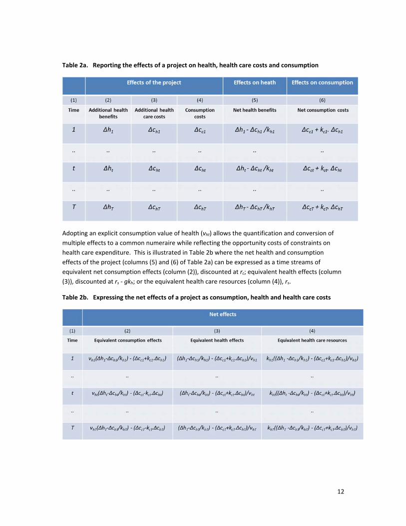
A project which has effects on health and health care costs but also imposes costs on private 

consumption (∆cct ), or offers private consumption benefits (when ∆cct  <0), is illustrated in Table 2a.  

The time stream of health benefits net of the health opportunity losses in column (5) combines the 

health benefits and additional health care costs of the project.  The net effect on consumption (in 

column (6)) is the consumption costs (column (4)) net of the consumption opportunity costs 

associated with additional health care costs and the health opportunity losses associated with them. 

Therefore, once other effects beyond health and health care costs are included, some assessment of 

the consumption opportunity costs of health care expenditure (kct), or the consumption effects of 

changes in health, is also required9.  The net effects of the project can then be reported as two time 

streams of net health and net consumption effects (columns (5) and (6)).10   

 

 

 

 

 

 

                                                            9 These alternatives will be equivalent if the causal consumption effects of health care expenditure run only through the health effects of health expenditure, rather than, in part at least, directly from health expenditure itself.  Insofar as health expenditure has a positive impact on economic growth compared to other forms of expenditure then restricting attention to the consumption effects of changes in health is likely to underestimate the consumption opportunity costs of health care costs.    10 It should be noted that attempts to estimate and explicitly account for the consumption opportunity costs of health care expenditure are particularly limited, even in high income settings, but do exist (Claxton et al 2015b). Although there is currently little evidence in lower income setting to support such assessment some default assumptions based on what is already known about the relationship between changes in health and economic growth should be possible. 

12  

 

Table 2a.   Reporting the effects of a project on health, health care costs and consumption 

 

Adopting an explicit consumption value of health (vht) allows the quantification and conversion of 

multiple effects to a common numeraire while reflecting the opportunity costs of constraints on 

health care expenditure.  This is illustrated in Table 2b where the net health and consumption 

effects of the project (columns (5) and (6) of Table 2a) can be expressed as a time streams of 

equivalent net consumption effects (column (2)), discounted at rc; equivalent health effects (column 

(3)), discounted at rs ‐ gkh; or the equivalent health care resources (column (4)), rs.   

Table 2b.   Expressing the net effects of a project as consumption, health and health care costs 

 

 

 

13  

2.2  The objective of the project is to improve welfare 

Traditionally the economic evaluation of social projects (e.g., Boadway and Bruce, 1984) adopts a 

view of social welfare resting on individual preferences revealed through markets or modified by an 

explicit welfare function. BCA is often founded on this more traditional approach and regards the 

purpose of any type of project, including those that require health care resources, as improving a 

broader notion of welfare rather than health or other explicitly stated social objectives.  This type of 

analysis tends to be less well represented in the evaluation of health projects, partly due to the 

difficulty of decision making bodies being willing to identify a welfare function carrying some broad 

consensus, particularly if health is felt to be unlike other goods (e.g., Broome 1978, Sen 1979, 

Brouwer et al., 2008, Arrow 2012). Nevertheless, health must inevitably be traded with other 

welfare arguments, most notably consumption, by social planners whilst taking account of the 

constraints on health and other public expenditure they face.   

BCA reports time streams of benefits and costs as their equivalent consumption values which 

represent the amount of consumption required to compensate for the costs of the project and the 

additional consumption that would need to be given to forego the benefits offered.  The results of 

this type of analysis can be reported as the benefit cost ratio or net present value of the project. If 

consumption and health are the only arguments or are separable from others (Gravelle et al., 2007) 

then the time stream of equivalent net consumption effects of the project illustrated in Table 2b 

(see column (2)) or the equivalent consumption value of the benefits and costs of the project 

illustrated in Table 1 (see columns (8) and (9)) are the estimates required for a BCA of these projects.  

Conducting analysis in this extensive way (illustrated in Table 1, 2a and 2b) ensures that any changes 

in the consumption value of health benefits and losses (vht) are already explicitly included in how the 

time streams of effects have been valued.  Similarly any expected changes in the health and other 

opportunity costs of health care expenditure (kht, kct) have already been explicitly accounted for in 

the time stream of health and consumption effects (see column (2) of Table 2b).    Once all the 

health and consumption effects of the project are expressed as equivalent time streams of 

consumption they can be discounted at a social time preference (STP) for consumption (rc).  The sum 

of the discounted time stream of the equivalent net consumption effects is the net present value of 

the project.  

An alternative to this more extensive approach would be to try and account for changes the 

consumption value of health and the opportunity costs of health care expenditure through 

discounting.  For example, for the project illustrated in Table 1, the discount rate for Δht could be 

amended to reflect expected growth in the consumption value of health, gvh, by reducing the 

discount rate applied to health benefits (rc – gvh). The discount rate applied to Δcht would also need 

to be amended to reflect both growth in the consumption value of health opportunity losses and any 

expected growth in a ‘threshold’ that reflects the health opportunity costs of heath expenditure (rc – 

gvh + gkh) (Claxton et al., 2011).11 This differential or dual discounting implicitly accounts for changes 

in the value of health and changes in the marginal productivity of health expenditure as well as time 

preference. This and other form of dual discounting creates potential for confusion and becomes 

more difficult when changes in the consumption opportunity costs of health care expenditure must 

be accounted for and when these parameters do not grow at a constant rate. The separate and 

                                                            11 This approximation is based on the plausible assumption that rh ,  gv and gk are small. 

14  

explicit accounting for each of these effects illustrated in Table 2b would appear more transparent, 

accountable and comparable.12  

How to think about time preference for equivalent consumption effects is well established and well 

worked through the Ramsey Rule (rc=δ + ηgc).  This includes pure time preference (δ, i.e., time 

preference for utility) and a wealth effect (ηgc) which reflects the relative weight attached to 

consumption in future compared to the current period.  Although an individual might exhibit forms 

of pure time preference there are good, albeit disputed, normative reasons to set pure time 

preference aside when making social choices that will have effects on current and future populations 

(Stern 2008, Nordhaus 2007, Arrow et al. 1999).  The wealth effect in the Ramsey Rule requires 

some assessment of the growth in future consumption (gc) and the weight that ought to be attached 

to them (η). This can be cast in a number of ways (e.g., based on individual diminishing marginal 

utility of consumption) and appeal to different forms of evidence (Groom and Maddison, 2013). 

However when considering social choices about projects which have impacts on current and future 

populations it might be best thought of as a form of inequality aversion where expectations of future 

growth in consumption means that additional consumption for future beneficiaries should be given 

less weight than the same additional consumption for current beneficiaries for whom consumption 

is more limited.  The important thing to note is that rc will always be country specific because even if 

η is common (and it need not be) rc will it will be determined by expectations about future 

consumption growth which are likely to differ. 

2.3  What is the distinction between CEA and BCA? 

The explicit assessment of the relative value of other effects shows that the distinction between a 

CEA which accounts for wider effects and a BCA, which incorporates the opportunity of cost or 

shadow prices of existing constraints, is more apparent than real.     Both require the same 

assessment of the same key parameters in Tables 2a and 2b.  Although much of the applied work to 

inform decision making bodies has adopted a narrower health care system perspective (in part due 

to a concern for the perceived cost of conflicts with other important social objectives that are more 

difficult to fully specify and quantify) a broader ‘societal’ or multi sectoral perspective in CEA is 

possible and is required and recommended by a number of decision making bodies13.      

What distinguishes BCA and CEA is a choice of whether social values ought to reflect those implied 

by the outcome of legitimate processes (e.g., government setting budgets for health care) or a 

notion of welfare founded on individual preferences or an explicit welfare function. For example, the 

former suggests a social time preference for health of rs –gkh and the latter, rc – gvh. The distinction 

                                                            12 The UK DH and AAWG ‘best practice’ report suggests that health opportunity costs are dealt with explicitly and separately from discounting. Nonetheless they recommend a discount rate of 1.5% for health and health care costs and 3.5% for other effects, which embeds the expectation that the consumption value of health will grow at 2%. This happens to nullify the wealth effect in UK Treasury STP based on the Ramsey Rule.  13 Drummond et al 2015,  Section 4.5.3 page 112‐116.  For example NICE requires a primary analysis from the perspective of the health care system.  However, an analysis that includes other effects can be considered and are required for public health interventions and programs. Other decision making bodies in the Netherlands and Sweden require a broader perspective to be adopted as the primary analysis.  A societal perspective was recommended as reference case analysis by the Washington Panel (Gold et al. 1996) , alongside a health care system perspective is recommended in the reference case by the Washington Panel. The recent update to this guidance (Neumann et al 2016) recommends analysis from both a societal and health care system perspective. 

15  

is whether social value is expressed by kt or vt and whether it is the opportunity cost of financing 

health care or the welfare arguments that underpin the Ramsey Rule that justify discounting.14    

The purpose is not to recommend which choice ought to be made but to clearly set out the 

implications for the common parameters that need to be assessed. The implications for discounting 

policy, whether conducting BCA or CEA, is that it becomes even more difficult and opaque to try and 

embed all these relevant arguments in how health, health care and other costs are discounted.  The 

quantification and conversion of the time streams of multiple effects to a common numeraire 

(illustrated in Table 2a) avoids embedding multiple augments in the discount rate for health and 

health care costs. For example, when it is believed to be important to explicitly quantify other 

impacts beyond measures of health and public health expenditure it would be appropriate to 

convert all effects into time streams of their equivalent consumption gains and losses, while 

reflecting the opportunity costs of existing constraints.  These time streams of consumption benefits 

and costs can then be discounted at a social time preference rate for consumption based on the 

Ramsey Rule. The separate and explicit accounting for these arguments allows clarity about the 

parameters that need to be assessed, available evidence to be identified and used transparently and 

consistently, while preserving the possibility of accountable deliberation about evidence, values and 

unquantified arguments in decision making processes.  

 

3.   Evidence available to inform key parameters and possible default estimates   

The common conceptual framework for CEA and BCA set out in Section 2 identifies the key 

parameters that need to be assessed to express the time streams of multiple effects to a common 

numeraire of equivalent consumption gains and losses which can then be discounted at STP for 

consumption. Each of these parameters, including STP for consumption, are likely to be country 

specific.  As a consequence, the net present value of a project which has effects across a number of 

counties will be the sum of the country specific net present values (see Table 4)   

3.1   Health opportunity costs of health care expenditure (kht) 

The problem of estimating a cost‐effectiveness ‘threshold’ that represents expected health 

opportunity costs is the same as estimating the relationship between changes in health care 

expenditure and health outcome.15  Estimates of the marginal productivity of health expenditure in 

producing health (QALYs) are becoming available for some high income countries based on 

approaches to estimation which exploit within country data (Martin et al. 2008, Claxton et al. 2015a,   

Vallejo‐Torres et al. 2017, and Edney, et al. 2018).  The proportionate effect on all‐cause mortality of 

proportionate changes in health expenditure (outcome elasticities) have also been estimated in 

higher income countries (Andrews, et al. 2017, Vallejo‐Torres, et al. 2017 and Edney, et al. 2017 and 

Claxton Martin and Lomas, 2018) using similar approaches to estimation of within country data and 

have reported similar estimates.  This evidence from higher income settings can be used to give 

some indication of possible values in lower income countries (Woods et al 2016) based on a number 

of assumptions about income elasticity of demand for health and the relative ‘under funding’ of 

                                                            14 The actual differences may be modest if gk and gv are similar and the real rate at which government can borrow is regarded as a reasonable proxy for STPR as some argue it is (Council of Economic Advisers 2017). 15 See Drummond et al 2015 Section 4.3 page 83‐94; Section 4.3.3.1 page 95‐95 

16  

health care systems.  This type of extrapolation suggests that cost per DALY averted is likely to be 

less than 1 GDP per capita in middle income countries and substantially lower in low income 

countries.  

The effect of different levels of health care expenditure on mortality outcomes has been 

investigated in a number of published studies using country level data, many including LMICs (Gallet 

and Doucouliagos 2017). The challenge is to control for all the other reasons why mortality might 

differ between countries in order to isolate the causal effect of differences in health expenditure.  

This is a particular challenge even if available measures are complete, accurate and unbiased 

because health outcomes are likely to be influenced by expenditure (increases in expenditure 

improves outcomes), but outcomes are also likely to influence expenditure (poor outcomes prompt 

greater efforts and increased expenditure) (Nakamura et al, 2016). This problem of endogeneity, as 

well as the inevitable aggregation bias, risks underestimating the health effects of changes in 

expenditure.   

Instrumental variables have been used in a number of studies to try and overcome this problem and 

estimate outcome elasticities for all cause adult and child mortality, by gender, as well as survival, 

disability and DALYs (Bokhari et al, 2007).  These estimated elasticities have been used to provide 

country specific cost per DALY averted values for 123 countries, taking account of measures of a 

country’s infrastructure, donor funding, population distribution, mortality rates, conditional life 

expectancies (all by age and gender), estimates of disability burden of disease and total health care 

expenditure (Ochalek et al 2015).  These estimates have recently been updated and work is 

underway to assess how cost per DALY averted is likely to evolve with changes in health care 

expenditure and consumption growth (Ochalek et al 2017).   

Possible default estimates (kht) 

Despite considerable data and estimation challenges some initial quantitative assessment of health 

opportunity costs and how they are likely to evolve is possible based on the balance of evidence such 

as it is. Updated estimates for almost all LMICs for 2015 expenditure are now available which might 

provide useful initial default estimates. Initial projections of these estimates based on other published 

projections of health expenditure and consumption are also available (Ochalek et al 2017).    These 

initial country specific estimates can be refined and updated as other country specific estimates 

emerge, ideally using within country data where this is possible. 

3.2   Consumption opportunity costs of health care expenditure (kct) 

The consumption opportunity costs associated with health care expenditure requires either direct 

evidence of the impact of changes on health care expenditure on net production (i.e., the value of 

additional production net of additional consumption) or estimates of the impact that changes in 

health are likely to have on net production in the rest of the economy (which with evidence from 3.1 

the former can be derived from the latter). 

Attempts to estimate and explicitly account for these non‐health opportunity costs of health 

expenditure are particularly limited even in high income settings but do exist.16  There are no explicit 

                                                            16 For example, as part of efforts to inform value based pricing of branded medicines (DH 2010 NICE 2014), the DH undertook work to estimate the ‘wider social benefits’ associated with changes in health outcome which 

17  

estimates for other countries, but a wide literature already exists at a micro level (e.g., health and 

labour market outcomes) and at a macro level (e.g., health and economic growth) which could be 

marshalled to derive estimates of the likely productive effects of changes in health relevant to 

different setting.    These types of estimates could provide some default assessment of the net 

production effects likely to be associated with the particular type of health benefits offered by a 

project which has health effect. Importantly, they can also be linked to evidence of health 

opportunity costs in 3.1 to estimate the consumption opportunity costs of health care expenditure. 

Possible default estimates (kct) 

In the absence of marshalling existing but disparate evidence a default assumption of 1 (1$ spent on 

health care delivers 1$ in net production or consumption opportunities) might not be unreasonable, 

albeit conservative assumption in LMIC settings given the very limited evidence currently available. 

Although there is little evidence about  how this aspect of opportunity costs is likely to evolve, a 

default assumption that the real value of the net production effects of the health effects of changes 

in health expenditure will grow at the same rate as consumption may not be unreasonable.  

3.3  Consumption value of health and its evolution over time (vht)         

There is a large literature which has used stated preferences (contingent valuation and discrete 

choice experiments) to estimate the consumption value or willingness to pay for improvements in 

health (e.g., Pinto‐Prades 2009, Mason et al 2009).  Recent reviews of this literature reveal wide 

variation in values (Vallejo‐Torres et al, 2016; Ryen and Svensson, 2015;).  The estimates reflect the 

demand for health and imply what health care expenditure ought to be, rather than a ‘supply side’ 

assessment of health opportunity costs.  Most estimate how much consumption an individual is 

willing to give up to improve their own health.  A few try to elicit how much individuals believe 

society should pay to improve health more generally.  A wider literature, that extends beyond 

health, estimates the value of a statistical life (VSL) based on how much consumption individuals are 

willing to give up to reduce their mortality risk (Hammitt 2000, Robinson et al 2016).  Some studies 

are based on stated preferences (e.g., Lindhjelm 2011) but others identify situations where 

individuals make choices that imply a value, e.g. revealed preferences in the labour market.  A cost 

per DALY can be derived from these studies by making assumptions about age and gender 

distribution, conditional life expectancies and quality of life norms.   

Most of this literature reports values relevant to high income countries and other methods papers 

for the BCA reference case deal in more detail how a consumption value of health relevant to LMIC 

settings might be derived.  However, some patterns that emerge are also likely to be relevant to 

LMICs: estimates based on VSL studies tend to be higher than those based on willingness to pay for 

health; values are not proportional to the scale of health gains and differ depending on whether 

health gains are through quality improvement or survival benefits.   

Although there is limited direct empirical evidence which provides values in lower income settings 

there is some limited evidence about how values might evolve over time with growth in 

consumption.  Reviews of the literature that have investigated the relationship between the VSL and 

                                                                                                                                                                                         could be linked to evidence of health opportunity costs to estimate the net production opportunity costs of changes in health expenditure.  The evidence in the UK suggests that a marginal £ in the NHS budget provides 92p worth of net production gains (see Appendix B of Claxton et al 2015b). 

18  

income (e.g., Viscusi and Aldy 2003; and Hammitt and Robinson 2011) suggests that earlier cross 

sectional studies of wage‐risk premiums indicate income elasticities <1, but longitudinal or cohort 

studies typically estimate elasticities >1. (e.g., Costa and Kahn 2004). The reasons for these 

differences may be that cross‐sectional studies are more likely to reflect changes in realised income, 

whereas longitudinal or across cohort studies are more likely to capture the impact of permanent 

income (e.g., Getzen 2000; Aldy and Smyth 2014). Despite the empirical difficulties the balance of 

evidence suggests that the consumption value of health increases with income.  Assuming an income 

elasticity of demand of health between 1 and 2 may not be unreasonable.  

There are also sound theoretical reasons why the value of health would be expected to grow with 

consumption (e.g., Parsonage and Neuburger 1992, Gravelle and Smith 2001, Hall and Jones 2007).  

The intuition can be expressed in the same way as the expected increase in value of environmental 

goods; that the growth in consumption is likely to outstrip the growth in health so health will 

become scarcer relative to consumption.  Since consumption is an imperfect substitute for health 

the value of health will increase.  These arguments can be made using behavioural models of 

individual choices of health affecting activities over time e.g., purchasing health care.  The growth in 

the value of health will be determined by income growth, the income elasticity of demand for health 

care and the elasticity of the marginal productivity of health care.  Alternatively health can be 

included as a separate argument in a social welfare function where it is valued in its own right, in 

part, because a healthier state increases the marginal utility of income and an indirect effect through 

income due to uninsured health care costs and/or increased productivity of being in a healthier 

state.  These insights indicate there are compelling reasons to believe the consumption value of 

health will grow with income and it is likely to grow at a faster rate if there is a direct effect of health 

on utility and an indirect effect through income.   

Possible default estimates (vht) 

Although theoretical arguments point to a number of empirical questions, a simple but reasonable 

assessment of how vht is likely to evolve could be based on growth in consumption (which is already 

required and embedded in the wealth effect of the Ramsey Rule) and assumptions about the income 

elasticity of demand for health.  An income elasticity of demand for health of 1 might be a 

reasonable albeit conservative default assumption in which case vht would grow at the same rate as 

consumption.  This could be compared with a less conservative scenario based on income elasticity of 

2, where the value of health benefits and health opportunity costs would grow at twice the rate of 

consumption.  Other scenarios could be justified based on evidence that income elasticity is likely to 

differ in particular settings. 

3.4   Other constrained sectors (vxt/kxt) 

Health expenditure is not the only category of public expenditure which is constrained.  Therefore, 

the effects of a project on other types of public expenditure ought to reflect their opportunity costs 

in the same way as health expenditure.  One way to do this is to use the evidence that is available 

for the health sector to shadow price other form of public expenditure. Estimates of the 

consumption value of health tend to be higher than available estimates of a ‘supply side’ assessment 

of health opportunity costs (Vallejo‐Torres et al, 2016).  This suggests a common discrepancy 

between the demand and supply side of health care systems.  For example, if these estimates are 

regarded as an appropriate expression of social value, the difference between vht and kht would 

19  

indicate that health care from collectively pooled resources is ‘underfunded’ compared to individual 

preferences about health and consumption.17  It is consistent with the view that the public funding 

of health care is not matching individual preferences and public expectations of their health care 

system.  However, given the difficulties faced in the public financing of health care and the welfare 

losses associated with socially acceptable means of taxation this is what might be expected and 

especially so in lower income settings where the difficulties of public financing are more acute. The 

balance of evidence suggests that vht/kht > 1.  This ratio is the shadow price for public health 

expenditure, i.e., the value of health expenditure $ relative to private consumption $.  Therefore, 

estimates of vht and kht, which are already required, can also be used to shadow price other forms of 

public expenditure. 

Possible default estimates (vxt/kxt) 

Estimates of vht/kht in the health sector might be used to shadow price other forms of public 

expenditure (where the equivalent estimates for that sector are absent) since resource allocation and 

expenditure decisions by government and other ministries would be expected to equalise this ratio 

across sectors (x) given an overall constraint on total public expenditure, i.e., it may not be 

unreasonable to assume vht/kht = vxt/kxt when considering impacts on public sector x.  

3.5  Time preference for consumption (rc) 

A social time preference rate for consumption based on the Ramsey Rule (rc=δ + ηgc) includes pure 

time preference (δ) and a wealth effect (ηgc).   Although an individual might exhibit forms of pure 

time preference, there are good, albeit disputed, normative reasons to set pure time preference 

aside when making social choices that will have effects on current and future populations (Stern 

2008, Nordhaus 2007, Arrow et al. 1999).  The wealth effect in the Ramsey Rule reflects an 

assessment of the expected growth in consumption (gc) and the weight that ought to be attached to 

consumption in the future compared to the current period (η). This ‘weight’ can be founded on 

different forms of evidence but might be best thought of as a form of inequality aversion where 

expectations of growth in means that additional consumption for future beneficiaries should be 

given less weight than the same additional consumption for current beneficiaries for whom 

consumption is more limited.   

There is some empirical evidence to inform η in high income countries (Groom and Maddison 2013) 

which includes reviews of expert opinion (Drupp et al. 2015).  However, the balance of this evidence 

in high income settings suggests that there is some element of inequality aversion with values of 

1<η<2 not being unreasonable (Groom and Maddison 2013).  There are also possibilities of obtaining 

revealed values for η through other social choices (e.g., the progressivity of tax and benefit systems) 

(Evans and Sezer 2002) or focusing on growth in median income (Emmerling Groom and 

Wettingfield, 2017) rather than applying an estimated η to expected growth in mean income.   Little 

direct evidence of η exists for LMICs; nonetheless country specific default estimates of rc are possible 

because even if η is common (and it need not be) it will be determined by expectations about 

                                                            17 For example, the UK DH has adopted £15,000 per QALY to assess health opportunity costs and until recently £60,000 per QALY as an estimate of the consumption value of health based on deriving QALY effects from VSL estimates. This would suggest that one health care £ is worth £4 of private consumption effects, which is especially important when there are other impacts which fall outside constrained public expenditure. 

20  

economic growth which are likely to differ between countries with different expectations about 

economic growth. 

Possible default estimates 

A conservative default assumption to establish country specific estimates of rc would be to apply η =1 

to available estimates of gc (reported as expected growth in measures of national income per capita 

for that country), i.e., the discount rate applied to time streams of equivalent consumption effects is 

gc.   This could be compared with a less conservative scenario based on η =2, where rc would be twice 

the expected growth in consumption.  Other scenarios could be justified based on evidence or 

reasoning of why η is likely to differ in specific contexts or based on different judgements about the 

prospects of future economic growth by social planners.  As evidence for values of η specific to LMICs 

evolves and estimates of economics growth are revised these defaults can be updated. This can also 

be compared to a wealth effect based only on expected growth in median income where those are 

available.  

3.6  Catastrophic, macroeconomic and project specific risk   

Catastrophic risk 

Truly catastrophic risk is best thought of as the probability of an event which would mean that all 

public and private projects will have zero cost and benefits, i.e., an event that represents total 

catastrophe for the whole of society.  When cast in this way it excludes events which could be 

described as ‘catastrophic’ but where some recovery might be possible even if this requires 

assistance from others (other countries, global bodies).  This is important, as although a 

‘catastrophic’ event where recovery is possible may have a major impact on the costs and benefits of 

public and private projects, these impacts are unlikely to be the same for all projects.  Therefore, 

these types of ‘catastrophic’ but recoverable risks are best included in the evaluation of the project 

itself rather than being embedded in a common discount rate for consumption effects. 

There are sources for probabilities of truly catastrophic events where recovery would not be 

possible (Chapman 2004, Stern 2007).  The probabilities are relatively small and if included would 

add little to a common discount rate for consumption effects.  Given the other more influential 

sources of uncertainty in specifying reasonable default values for a common discount rate for 

consumption affects it might be reasonable to set aside truly catastrophic risks. If catastrophic risk is 

included, it should be based an estimate of the probabilities of truly catastrophic events where 

recovery would not be possible (≤0.1%).  

Macroeconomic risk 

When all effects of a project are expressed as streams of consumption benefits and costs then 

discounting using STP for consumption would be appropriate.  However, some decline in rc over 

longer time horizons will be required to reflect the impact of increasing uncertainty in rc  due to 

uncertainty in the consumption growth element of the wealth effect of the Ramsey Rule.  (Arrow et 

al. 2013, Cropper et al. 2014, Freeman and Groom 2016, Freeman et al 2015). Since uncertainty in rc 

will increase over time, due to increasing uncertainty about future consumption, some decline is 

21  

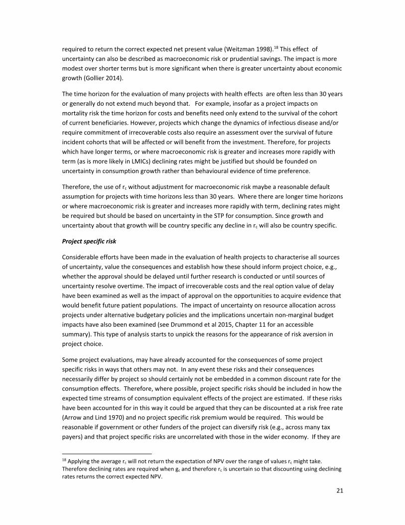
required to return the correct expected net present value (Weitzman 1998).18 This effect  of 

uncertainty can also be described as macroeconomic risk or prudential savings. The impact is more 

modest over shorter terms but is more significant when there is greater uncertainty about economic 

growth (Gollier 2014).  

The time horizon for the evaluation of many projects with health effects  are often less than 30 years 

or generally do not extend much beyond that.   For example, insofar as a project impacts on 

mortality risk the time horizon for costs and benefits need only extend to the survival of the cohort 

of current beneficiaries. However, projects which change the dynamics of infectious disease and/or 

require commitment of irrecoverable costs also require an assessment over the survival of future 

incident cohorts that will be affected or will benefit from the investment. Therefore, for projects 

which have longer terms, or where macroeconomic risk is greater and increases more rapidly with 

term (as is more likely in LMICs) declining rates might be justified but should be founded on 

uncertainty in consumption growth rather than behavioural evidence of time preference. 

Therefore, the use of rc without adjustment for macroeconomic risk maybe a reasonable default 

assumption for projects with time horizons less than 30 years.  Where there are longer time horizons 

or where macroeconomic risk is greater and increases more rapidly with term, declining rates might 

be required but should be based on uncertainty in the STP for consumption. Since growth and 

uncertainty about that growth will be country specific any decline in rc will also be country specific. 

Project specific risk 

Considerable efforts have been made in the evaluation of health projects to characterise all sources 

of uncertainty, value the consequences and establish how these should inform project choice, e.g., 

whether the approval should be delayed until further research is conducted or until sources of 

uncertainty resolve overtime. The impact of irrecoverable costs and the real option value of delay 

have been examined as well as the impact of approval on the opportunities to acquire evidence that 

would benefit future patient populations.  The impact of uncertainty on resource allocation across 

projects under alternative budgetary policies and the implications uncertain non‐marginal budget 

impacts have also been examined (see Drummond et al 2015, Chapter 11 for an accessible 

summary). This type of analysis starts to unpick the reasons for the appearance of risk aversion in 

project choice. 

Some project evaluations, may have already accounted for the consequences of some project 

specific risks in ways that others may not.  In any event these risks and their consequences 

necessarily differ by project so should certainly not be embedded in a common discount rate for the 

consumption effects.  Therefore, where possible, project specific risks should be included in how the 

expected time streams of consumption equivalent effects of the project are estimated.  If these risks 

have been accounted for in this way it could be argued that they can be discounted at a risk free rate 

(Arrow and Lind 1970) and no project specific risk premium would be required.  This would be 

reasonable if government or other funders of the project can diversify risk (e.g., across many tax 

payers) and that project specific risks are uncorrelated with those in the wider economy.  If they are 

                                                            18 Applying the average rc will not return the expectation of NPV over the range of values rc might take.  Therefore declining rates are required when gc and therefore rc is uncertain so that discounting using declining rates returns the correct expected NPV. 

22  

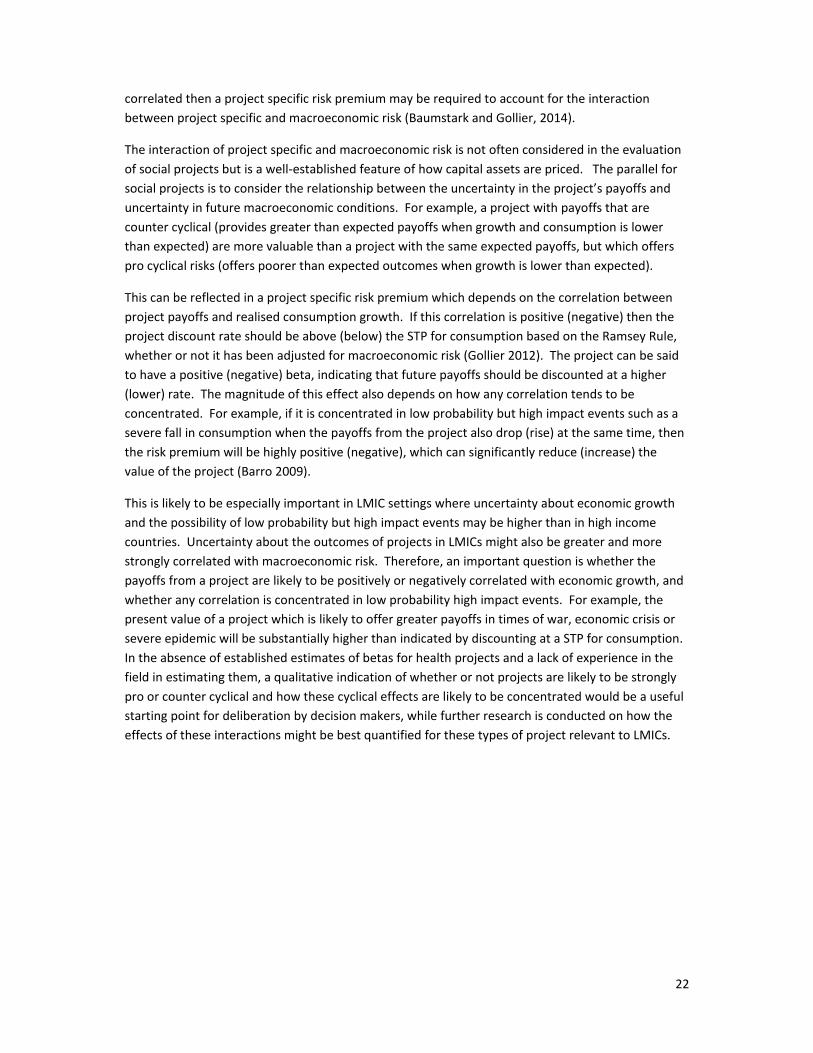
correlated then a project specific risk premium may be required to account for the interaction 

between project specific and macroeconomic risk (Baumstark and Gollier, 2014).   

The interaction of project specific and macroeconomic risk is not often considered in the evaluation 

of social projects but is a well‐established feature of how capital assets are priced.   The parallel for 

social projects is to consider the relationship between the uncertainty in the project’s payoffs and 

uncertainty in future macroeconomic conditions.  For example, a project with payoffs that are 

counter cyclical (provides greater than expected payoffs when growth and consumption is lower 

than expected) are more valuable than a project with the same expected payoffs, but which offers  

pro cyclical risks (offers poorer than expected outcomes when growth is lower than expected).   

This can be reflected in a project specific risk premium which depends on the correlation between 

project payoffs and realised consumption growth.  If this correlation is positive (negative) then the 

project discount rate should be above (below) the STP for consumption based on the Ramsey Rule, 

whether or not it has been adjusted for macroeconomic risk (Gollier 2012).  The project can be said 

to have a positive (negative) beta, indicating that future payoffs should be discounted at a higher 

(lower) rate.  The magnitude of this effect also depends on how any correlation tends to be 

concentrated.  For example, if it is concentrated in low probability but high impact events such as a 

severe fall in consumption when the payoffs from the project also drop (rise) at the same time, then 

the risk premium will be highly positive (negative), which can significantly reduce (increase) the 

value of the project (Barro 2009). 

This is likely to be especially important in LMIC settings where uncertainty about economic growth 

and the possibility of low probability but high impact events may be higher than in high income 

countries.  Uncertainty about the outcomes of projects in LMICs might also be greater and more 

strongly correlated with macroeconomic risk.  Therefore, an important question is whether the 

payoffs from a project are likely to be positively or negatively correlated with economic growth, and 

whether any correlation is concentrated in low probability high impact events.  For example, the 

present value of a project which is likely to offer greater payoffs in times of war, economic crisis or 

severe epidemic will be substantially higher than indicated by discounting at a STP for consumption. 

In the absence of established estimates of betas for health projects and a lack of experience in the 

field in estimating them, a qualitative indication of whether or not projects are likely to be strongly 

pro or counter cyclical and how these cyclical effects are likely to be concentrated would be a useful 

starting point for deliberation by decision makers, while further research is conducted on how the 

effects of these interactions might be best quantified for these types of project relevant to LMICs.  

 

 

 

 

 

 

23  

4  Recommendations, reporting and further research     

4.1  A summary possible default estimates 

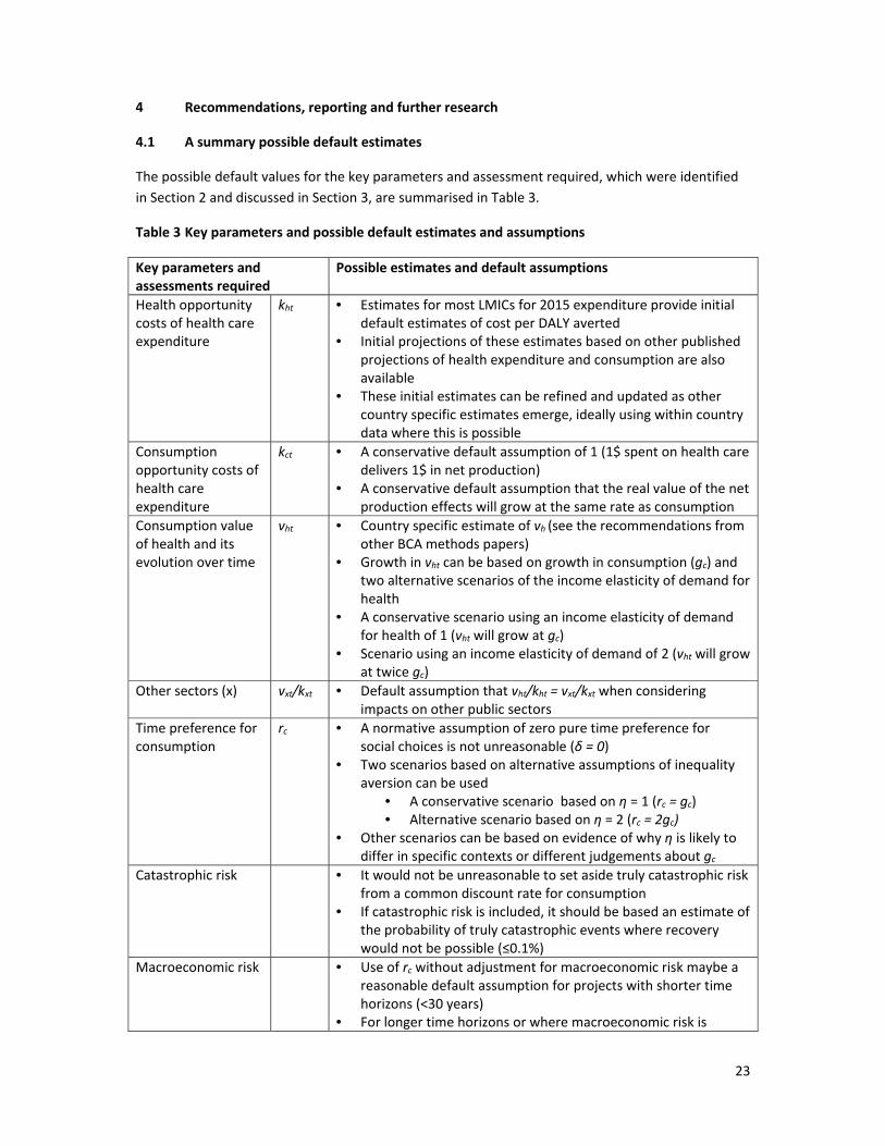
The possible default values for the key parameters and assessment required, which were identified 

in Section 2 and discussed in Section 3, are summarised in Table 3.   

Table 3 Key parameters and possible default estimates and assumptions 

Key parameters and assessments required 

Possible estimates and default assumptions 

Health opportunity costs of health care expenditure 

kht  

• Estimates for most LMICs for 2015 expenditure provide initial default estimates of cost per DALY averted 

• Initial projections of these estimates based on other published projections of health expenditure and consumption are also available    

• These initial estimates can be refined and updated as other country specific estimates emerge, ideally using within country data where this is possible 

Consumption opportunity costs of health care expenditure 

kct  

• A conservative default assumption of 1 (1$ spent on health care delivers 1$ in net production) 

• A conservative default assumption that the real value of the net production effects will grow at the same rate as consumption 

Consumption value of health and its evolution over time 

 

vht  

• Country specific estimate of vh (see the recommendations from other BCA methods papers) 

• Growth in vht can be based on growth in consumption (gc) and two alternative scenarios of the income elasticity of demand for health   

• A conservative scenario using an income elasticity of demand for health of 1 (vht will grow at gc) 

• Scenario using an income elasticity of demand of 2 (vht will grow at twice gc) 

Other sectors (x)   

vxt/kxt  

• Default assumption that vht/kht = vxt/kxt when considering impacts on other public sectors 

Time preference for consumption  

rc  

• A normative assumption of zero pure time preference for  social choices is not unreasonable (δ = 0) 

• Two scenarios based on alternative assumptions of inequality aversion can be used 

• A conservative scenario  based on η = 1 (rc = gc) • Alternative scenario based on η = 2 (rc = 2gc) 

• Other scenarios can be based on evidence of why η is likely to differ in specific contexts or different judgements about gc   

Catastrophic risk  

  • It would not be unreasonable to set aside truly catastrophic risk from a common discount rate for consumption 

• If catastrophic risk is included, it should be based an estimate of the probability of truly catastrophic events where recovery would not be possible (≤0.1%) 

Macroeconomic risk  

  • Use of rc without adjustment for macroeconomic risk maybe a reasonable default assumption for projects with shorter time horizons (<30 years) 

• For longer time horizons or where macroeconomic risk is 

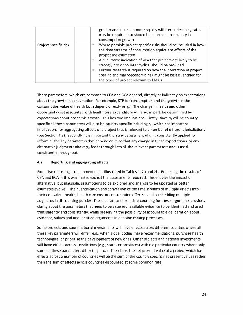
24  

greater and increases more rapidly with term, declining rates may be required but should be based on uncertainty in consumption growth 

Project specific risk    • Where possible project specific risks should be included in how the time streams of consumption equivalent effects of the project are estimated 

• A qualitative indication of whether projects are likely to be strongly pro or counter cyclical should be provided 

• Further research is required on how the interaction of project specific and macroeconomic risk might be best quantified for the types of project relevant to LMICs 

 

These parameters, which are common to CEA and BCA depend, directly or indirectly on expectations 

about the growth in consumption. For example, STP for consumption and the growth in the 

consumption value of health both depend directly on gc.  The change in health and other 

opportunity cost associated with health care expenditure will also, in part, be determined by 

expectations about economic growth.  This has two implications.  Firstly, since gc will be country 

specific all these parameters will also be country specific including rc , which has important 

implications for aggregating effects of a project that is relevant to a number of different jurisdictions 

(see Section 4.2).  Secondly, it is important than any assessment of gc is consistently applied to 

inform all the key parameters that depend on it, so that any change in these expectations, or any 

alternative judgments about gc, feeds through into all the relevant parameters and is used 

consistently throughout. 

4.2  Reporting and aggregating effects 

Extensive reporting is recommended as illustrated in Tables 1, 2a and 2b.  Reporting the results of 

CEA and BCA in this way makes explicit the assessments required. This enables the impact of 

alternative, but plausible, assumptions to be explored and analysis to be updated as better 

estimates evolve.   The quantification and conversion of the time streams of multiple effects into 

their equivalent health, health care cost or consumption effects avoids embedding multiple 

augments in discounting policies. The separate and explicit accounting for these arguments provides 

clarity about the parameters that need to be assessed, available evidence to be identified and used 

transparently and consistently, while preserving the possibility of accountable deliberation about 

evidence, values and unquantified arguments in decision making processes. 

Some projects and supra national investments will have effects across different counties where all 

these key parameters will differ, e.g., when global bodies make recommendations, purchase health 

technologies, or prioritise the development of new ones. Other projects and national investments 

will have effects across jurisdictions (e.g., states or provinces) within a particular country where only 

some of these parameters differ (e.g.,  kht).  Therefore, the net present value of a project which has 

effects across a number of countries will be the sum of the country specific net present values rather 

than the sum of effects across countries discounted at some common rate.   

 

 

25  

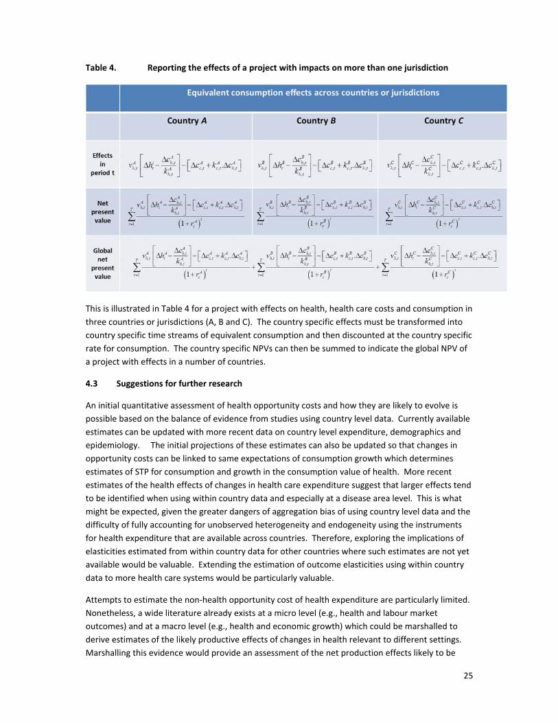
Table 4.  Reporting the effects of a project with impacts on more than one jurisdiction   

 

This is illustrated in Table 4 for a project with effects on health, health care costs and consumption in 

three countries or jurisdictions (A, B and C).  The country specific effects must be transformed into 

country specific time streams of equivalent consumption and then discounted at the country specific 

rate for consumption.  The country specific NPVs can then be summed to indicate the global NPV of 

a project with effects in a number of countries.   

4.3   Suggestions for further research 

An initial quantitative assessment of health opportunity costs and how they are likely to evolve is 

possible based on the balance of evidence from studies using country level data.  Currently available 

estimates can be updated with more recent data on country level expenditure, demographics and 

epidemiology.     The initial projections of these estimates can also be updated so that changes in 

opportunity costs can be linked to same expectations of consumption growth which determines 

estimates of STP for consumption and growth in the consumption value of health.  More recent 

estimates of the health effects of changes in health care expenditure suggest that larger effects tend 

to be identified when using within country data and especially at a disease area level.  This is what 

might be expected, given the greater dangers of aggregation bias of using country level data and the 

difficulty of fully accounting for unobserved heterogeneity and endogeneity using the instruments 

for health expenditure that are available across countries.  Therefore, exploring the implications of 

elasticities estimated from within country data for other countries where such estimates are not yet 

available would be valuable.  Extending the estimation of outcome elasticities using within country 

data to more health care systems would be particularly valuable.  

Attempts to estimate the non‐health opportunity cost of health expenditure are particularly limited.  

Nonetheless, a wide literature already exists at a micro level (e.g., health and labour market 

outcomes) and at a macro level (e.g., health and economic growth) which could be marshalled to 

derive estimates of the likely productive effects of changes in health relevant to different settings.    

Marshalling this evidence would provide an assessment of the net production effects likely to be 

26  

associated with the particular type of health benefits offered by a project as well as the net 

production losses from the health opportunity costs associated with the projects demands on health 

care expenditure. 

Estimates of country specific expected growth in consumption are available and can inform a 

number of parameters including STP for consumption. Although there is some empirical evidence to 

inform the weight that might be attached to future compared to current consumption (η), little 

direct evidence of exists for LMICs.  There are, however, possibilities of obtaining revealed values for 

η through other social choices (e.g., the progressivity of tax and benefit systems) or focusing on 

growth in median income rather than applying an estimated η to growth in mean income. It would 

be useful to review existing estimates of median income in LMICs and examine how its expected 

growth might be linked to current estimates of economic growth.  This would enable alternative 

ways to estimate a STP for consumption to be considered. The evidence to support estimates of the 

consumption value of health in particular LMICs and income elasticities of demand for health are 

also limited. Other BCA methods papers consider in more detail how these might be estimated in 

LMICs and discuss further research that might be conducted. 

The use of rc without adjustment for increasing uncertainty about future consumption maybe a 

reasonable default assumption for projects with shorter time horizons.  However, for longer time 

horizons or where macroeconomic risk is greater and increases more rapidly with term (as is more 

likely in LMICs) declining rates might be required. A review of estimates of gc relevant to LMICs could 

identify the circumstances where declining rates should be applied.  This could be used to develop 

tools which would provide appropriate declining rates for rc based on gc, measures of uncertainty in 

gc by term, η and an initial assumption that projects are neither pro or counter cyclical (beta=0).   

An important question is whether the payoffs from a project are likely to be positively or negatively 

correlated with economic growth, and whether any correlation is concentrated in low probability 

high impact events.  Such correlation and the project risk premiums they imply can have a significant 

impact on the value of a project.  This issue is not often considered in the evaluation of social 

projects and there is a lack of experience of estimating this type of risk premium (betas) for the 

types of projects considered in LMICs.  Therefore, a first step would be to illustrate, with case 

studies, how a qualitative indication of whether or not projects are likely to be strongly pro or 

counter cyclical might be made and how these cyclical effects are likely to be concentrated.  This 

might also identify the characteristics of projects and circumstances where quantifying the 

interaction of project and macroeconomic risk is likely to be particularly important in project choice 

and how betas might be estimated for these types of project. 

 

 

 

 

 

 

27  

References 

Aldy, J.E., Smyth, S.J. (2014) Heterogeneity in the value of life. Resources for the Future, Discussion 

Paper No. 14‐13. 

Andrews, M. et al. (2017) Inference in the presence of redundant moment conditions and the impact 

of government health expenditure on health outcomes in England. Econometric Reviews, 36(1–3), 

pp.23–41. 

Arrow K, R Lind (1970). Uncertainty and the evaluation of public investment decisions. American 

Economic Review, 60, 364–378. 

Arrow, K.J. (2012) Social Choice and Individual Values, with an introduction by Eric S Maskin, 

Newhaven: Cowles Foundation; 2012. 

Arrow K, M Cropper, C Gollier, B Groom, G Heal, R Newell, W Nordhaus, R Pindyck, W Pizer, P 

Portney, T Sterner, R Tol, M Weitzman (2013). Determining benefits and costs for future 

generations. Science, 341(6144), 349–50. 

Barro RJ (2009). Rare disasters, asset prices, and welfare costs. American Economic Review, 99, 243–

264. 

Baumstark L, C Gollier (2014). The relevance and the limits of the Arrow‐Lind Theorem.  Journal of 

Natural Resources Policy Research, 6, 45–49. 

Bertram, M.Y. et al. (2016) Use and misuse of thresholds Cost–effectiveness thresholds: pros and 

cons. Bulletin of the World Health Organization. Dec 1; 94(12): 925–930. 

Boadway RW, Bruce N. (1984). Welfare Economics. Blackwell: Oxford. 

Bokhari FAS, Gai Y, Gottret P. (2007) Government health expenditures and health outcomes. Health 

Economics, 16: 257‐273. 

Broome, J. (1978). Trying to value a life. Journal of Public Economics, 9, 91–100. 

Brouwer WBF, Niessen LW, Postma MJ, Rutten FFH. (2005) Need for differential discounting of costs 

and health effects in cost effectiveness analyses. British Medical Journal 331: 446‐448. 

Brouwer W, Culyer AJ, Job N, van Exel A, Rutten FH. (2008). Welfarism vs. extra‐welfarism. Journal of 

Health Economics, 27: 325–338. 

Chapman CR. (2004). The hazard of near‐Earth asteroid impacts on earth. Earth Planet Sci Lett., 

222(1):1‐15 

Claxton, K, Paulden, M, Gravelle, H, Brouwer, W & Culyer, AJ (2011). Discounting and decision 

making in the economic evaluation of health‐care technologies' Health Economics, 20(1): 2‐15. 

Claxton K, Martin S, Soares MO, Rice N, Spackman E, Hinde S, Devlin N, Smith PC, Sculpher M. 

(2015a). Methods for the estimation of the NICE cost effectiveness threshold. Health Technology 

Assessment, 19(14). 

28  

Claxton K, Sculpher M, Palmer S, Culyer AJ. (2015b). Causes for concern: is NICE failing to uphold its 

responsibilities to all NHS patients? Health Economics, 24(1):1‐7. 

Claxton K, Lomas JRS, Martin S. (2018).The impact of NHS expenditure on health outcomes in 

England: Alternative approaches to identification in all‐cause and disease specific models of 

mortality. Health Economics. Feb 7. 

Coast, J., Smith, R., and Lorgelly, P. (2008), 'Welfarism, extra‐welfarism and capability: the spread of 

ideas in health economics', Social Science and Medicine, 67, 1190‐98. 

Costa DL, Kahn ME.  (2004). Changes in the value of life, 1940–1980. Journal of Risk and Uncertainty, 

XXIX, 159–180. 

Council of Economic Advisers Discounting for public policy: theory and recent evidence on the merits 

of updating the discount rate. Council of Economic Advisers Issue Brief, January 2017. 

Cropper M, MC Freeman, B Groom, W Pizer (2014). Declining discount rates. American Economic 

Review: Papers & Proceedings, 104, 538–543. 

Culyer AJ, McCabe C, Briggs A, Claxton K, Buxton M, Akehurst R, Sculpher M, Brazier J. (2007). 

Searching for a threshold, not setting one: the role of the National Institute of Health and Clinical 

Excellence. Journal of Health Services Research and Policy 12: 56‐58. 

Department of Health. 2004. Policy Appraisal and Health: A Guide from the Department of Health 

(Reissued). Department of Health: London. 

Drummond MF, Sculpher MJ, Claxton K, Stoddart GL, Torrance GW. (2015). Methods for the 

Economic Evaluation of Health Care Programmes. 4th ed. Oxford: Oxford: Oxford University Press. 

Edney, LC. et al. (2018). Estimating the Reference Incremental Cost‐Effectiveness Ratio for the 

Australian Health System. Pharmacoeconomics. Feb;36(2):239‐252. 

Emmerling J, Groom B and Wettingfield T (2017) Discounting and the representative median agent. 

Economics Letters, 161. pp. 78‐81 

Evans D J and Sezer H (2002). A time preference measure of the Social Discount Rate for the UK. 

Applied Economics, 34, 1925‐1934. 

Freeman MC, B Groom (2016). How certain are we about the certainty‐equivalent long term social 

discount rate?  Journal of Environmental Economics and Management.  Online at doi: 

http://dx.doi.org/10.1016/j.jeem.2016.06.004 

Freeman MC, B Groom, E Panopoulou, T Pantelidis (2015). Declining discount rates and the Fisher 

Effect: Inflated past, discounted future? Journal of Environmental Economics and Management, 73, 

32‐49. 

Gallet, C.A. & Doucouliagos, H. (2017) The impact of healthcare spending on health outcomes: A 

meta‐regression analysis. Social Science & Medicine. 179, pp.9–17. 

29  

Getzen, T.E. (2000) Health care is an individual necessity and a national luxury: applying multilevel 

decision models to the analysis of health care expenditures. J Health Econ. 19(2): p. 259‐70. 

Gollier C (2012). Evaluation of long‐dated investments under uncertain growth trend, volatility and 

catastrophes. CESifo Working Paper: Industrial Organisation, No. 4052. 

Gollier C (2014). Discounting and growth. American Economic Review: Papers & Proceedings, 104, 

534–537. 

Gravelle H, Smith D. (2001). Discounting for health effects in cost‐benefit and cost‐effectiveness 

analysis. Health Economics 10: 587‐599. 

Gravelle H, Brouwer WBF, Niessen LW, Postma MJ, Rutten FFH. (2007). Discounting in economic 

evaluations: stepping forward towards optimal decision rules. Health Economics 16(3): 307‐317. 

Groom B, DJ Maddison (2013). Non‐identical quadruplets: Four new estimates of the elasticity of 

marginal utility for the UK. Centre for Climate Change Economics and Policy Working Paper No. 141. 

Hall RE, Jones CI. (2007). The value of life and the rise in health spending. Quarterly Journal of 

Economics, February, Vol. 122 (1), pp. 39‐72. 

Hammitt JK. 2000. Valuing mortality risk: theory and practice. Environmental Science and 

Technology 34: 1396–400. 

Hammitt, J.K., Robinson, L.A. (2011). The income elasticity of the value per statistical life: 

transferring estimates between high and low income populations. Journal of Benefit‐Cost Analysis, 

2(1): p. 2152‐2812. 

Lipscomb J, Weinstein MC, Torrance GW. (1996). Time preference. In Cost‐Effectiveness in Health 

and Medicine, Gold MR, Siegel JE, Russell LB, Weinstein MC (eds). Oxford University Press: Oxford, 

214–246. 

Lindhjelm H, Navrud S, Braathen NA, Biausque V. 2011. Valuing mortality risk reductions from 

environmental, transport, and health policies: a global meta‐analysis of stated preference studies. 

Risk Analysis 31: 1381–1407. 

Mason H, Jones‐Lee M, Donaldsson C. (2009). Modelling the monetary value of a QALY: a new 

approach based on UK data. Health Economics 18: 933–950. 

Meltzer, D. O. (2013), 'Future costs in medical cost‐effectiveness analysis ', in A. Jones (ed.), The 

Elgar Companion to Health Economics (Cheltenham: Edward Elgar Publishing Ltd), 481‐89. 

Nakamura R, Lomas JRS, Claxton K, Bokhari F, Moreno Serra RA, Suhrcke ME. Assessing the impact of 

health care expenditures on mortality using cross‐country data. (2016). York, UK: Centre for Health 

Economics, University of York. Apr, p. 1‐57. (CHE Research Paper; 128). 

Neumann PJ, Sanders GD, Russell LB, Siegel JE, Ganiats TG, editors. Cost‐effectiveness in health and 

medicine. Second edition. 2nd edition. New York: Oxford University Press; 2016. 

30  

Nord, E. (2011), Discounting future health benefits: the poverty of consistency arguments. Health 

Economics, 20, 16–26. 

Nordhaus WD. (2007). A review of the Stern review on the economics of climate change. J Econ Lit., 

45(3):686‐702. 

Ochalek JM, Lomas J, Claxton K. (2015). Cost per DALY averted thresholds for low‐ and middle‐

income countries: evidence from cross country data. York, UK: Centre for Health Economics, 

University of York. Dec, p. 1‐50. (CHE Research Paper; 122). 

Parsonage M, Neuburger H. (1992). Discounting and  health benefits. Health Econ, 1: 71–76. 

Paulden, M. and Claxton, K.   (2012), 'Budget allocation and the revealed social rate of time 

preference for health', Health Economics, 21, 612‐18. 

Paulden M, O’Mahony JF, and McCabe C. (2017). Discounting the Recommendations of the Second 

Panel on Cost‐Effectiveness in Health and Medicine. PharmacoEconomics, 35:5–13 

Paulden M, Galvanni V, Chakraborty S, Kudinga B, McCabe C. Discounting and the Evaluation of 

Health Care Programmes.CADTH. 2016. 

https://www.cadth.ca/sites/default/files/pdf/CP0008_Economic_Evaluation_Guidelines_Discount_R

ate_Report.pdf 

Pinto‐Prades JL, Loomes G, Brey R. (2009). Trying to estimate a monetary value for the QALY. Journal 

of Health Economics 28: 553–562. 

Phelps, C.E. and Mushlin, A.I. (1991), On the (near) equivalence of cost‐effectiveness and cost‐

benefit analyses. International Journal of Technology Assessment in HeaIth Care, 7, 12‐21. 

Rawlins, M. D.  and Culyer, A. J. (2004), National Institute for Clinical Excellence and its value 

judgments. British Medical Journal, 329, 224 ‐ 27. 

Robinson LA, Hammitt JK, Chang AJ, and Resch S. (2016). Understanding and improving the one and 

three times GDP per capita cost‐effectiveness thresholds. Health Policy Planning. First published 

online: July 24, 2016. 

Ryen, L.  and Svensson, M. (2014), 'The willingness to pay for a quality‐adjusted life year: a review of 

the empirical literature DOI: 10.1002/hec.3085', Health Economics. 

Sen, A. (1979), Personal utilities and public judgments. Or what's wrong with welfare economics. The 

Economic Journal, 89, 537–58. 

Spackman M. (2017). Social discounting: the SOC/STP divide. Grantham Research Institute on 

Climate Change and the Environment, Working Paper No. 182, February. 

Stern NH (2007). The economics of climate change: the Stern review. Cambridge University Press, 

Cambridge, UK. 

Stern NH (2008). The economics of climate change. Am Econ Rev. May;98(2):1‐37. 

31  

Stinnett AA, Mullahy J. (1998). Net health benefits: a new framework for the analysis of uncertainty 

in cost‐effectiveness analysis. Medical Decision Making 18(suppl): S68‐S80. 

Martin S, Rice N, Smith PC. (2012). Comparing costs and outcomes across programmes of health 

care. Health Economics. Mar;21(3):316‐337. 

Martin S, Rice N, and Smith PC. (2008). Does health care spending improve health outcomes? 

Evidence from English programme budgeting data. Journal of Health Economics, 27:826–42. 

Vallejo‐Torres L, García‐Lorenzo B, Castilla I, Valcárcel‐Nazco C, Lidia García‐Pérez L, Linertová R, 

Polentinos‐Castro E, Pedro Serrano‐Aguilar P.(2016).  On the Estimation of the Cost‐Effectiveness 

Threshold: Why, What, How? Value in Health. First published online: 23 April, 2016. 

Viscusi, W.K. and Aldy JE. (2003). The value of a statistical life: A critical review of market estimates 

throughout the world. Journal of Risk and Uncertainty, 27(1): p. 5‐76. 

Woods BS, Revill P, Sculpher MJ, Claxton K. (2016). Country‐level cost‐effectiveness thresholds: 

initial estimates and the need for further research. Value in Health, Feb 20.