Timing is Everything? An Empirical Analysis of the

Timing is Everything? An Empirical Analysis of the Determinants of

Service Quality Provision∗

Olivier Chatain†

The Wharton SchoolThe University of Pennsylvania

Alon Eizenberg‡

Department of EconomicsHebrew University of Jerusalem

March 2014

Abstract

We utilize a unique database from a large legal services provider to examine how service qualityresponds to the firm’s available capacity, and to the nature of the firm-client relationship. We developempirical measures of both the (internal) level of resources available to the firm at different pointsin time, and of the (external) value creation for customers. Our results indicate that service qualityincreases in the amount of the firm’s available resources, suggesting that quality adjustment can beused as a means of tackling capacity constraints. We also find that service quality increases in thenumber of previous successful interactions with the client, implying that the firm strategically investsin building long-term relationships with clients. By documenting these relationships, we wish to shedlight on the limitations of current estimates of consumer surplus in service industries, as well as onpotential inefficiencies in such industries.

Keywords: Resource Allocation, Endogenous quality.

∗We thank the managers of the legal service provider for giving us access to the data and for their time and patienceduring the development of the paper. We thank Dan Ben Moshe for comments and suggestions. Kostia Kofman providedexcellent research assistance.†[email protected]‡[email protected]

1 Introduction

Two important features often characterize a firm’s competitive environment. First, the level of

demand faced by the firm may be uncertain and fluctuating, such that the firm may not be

able to perfectly forecast the number of clients it would need to serve at a given point in time.

Second, the firm may face capacity constraints that restrict its short-run production of goods

and services. These two features, put together, create a tradeoff with respect to the firm’s choice

of its capacity level: choosing a high capacity level would result in much of this large capacity

being idle on low-demand periods, whereas choosing a low capacity level would not allow the

firm to meet its demand on high-demand periods.

Firms may tackle such short run capacity constraints by adjusting prices. Setting a high (low)

price in high (low) demand periods enables the firm to adjust the quantity demanded taking into

account its available capacity. Such management of price is routinely practiced by airlines. In

many cases, however, this degree of freedom is not available: prices may be difficult to adjust in

competitive sectors, in industries where price controls are in place, or in cases where the cost of

changing prices is high.

As an alternative to adjusting prices, the firm may consider adjusting the quality of its goods

and services. While product quality is often fixed or hard to change in the case of physical

products, firms providing professional services have a lot of leeway in determining service qual-

ity. For instance, a firm may reduce the amount of attention and resources spent on clients

on high-demand periods, making it possible to meet this high demand given a fixed capacity.

Such a strategy may be reflected in spending only a limited amount of time in an attempt to

understand the customer’s specific situation and needs, or by restricting the use of more senior

professionals in favor of junior ones. In professional service industries (e.g., consulting, legal ser-

vices, investment banking advisory), this channel may be an attractive option, especially since

firms in such industries may be wary to compete on price for a variety of reasons. For example,

the firm may view its rates as a long-term, stable signal of its reputation, and may therefore

refrain from adjusting it at a high frequency.

In this paper we utilize a unique dataset from a provider of legal services to study the extent to

which the level of service enjoyed by a client varies with the firm’s available capacity, the client’s

characteristics and the nature of the firm-client relationship. Our empirical strategy develops a

couple of measures of service quality, and then relates these measures to explanatory variables

at the individual client level. This allows us to address a number of interesting questions.

First, motivated by the discussion above, we ask whether service quality is higher in situations

in which the firm has more relevant resources at its disposal. We find that this is, indeed,

the case. This finding has a couple of important implications. First, it illuminates important

limitations of typical studies that measure output and welfare in service industries. Consider, for

2

example, two clients who get an annual checkup for their automobiles at a garage, each of them

paying 80 US$. One of them, however, arrived on a “good” day when the garage was not too

busy, and had a better and more careful job done on her car. Studies that measure output and

consumer welfare would not typically consider this possibility and would treat both transactions

symmetrically.

While a considerable body of research in economics (notably Griliches 1961, Pakes 2003)

emphasizes the importance of computing quality-adjusted indices of physical output, the literature

remains largely silent on the issue of how to measure service quality and account for the possibility

that clients arriving at different times may enjoy different service levels. Researchers may be able

to control for quality differences arising from the service being rendered by different providers

at different prices. Accounting for quality differences across transactions performed with the

same provider, and at the same price, is a much more ambitious challenge that is typically

ignored. Our paper, while having the limitation of providing evidence from one specific firm,

uses the specificity of the setup in order to provide a detailed analysis and measurement of

quality, revealing that such within-provider quality differences are indeed observed. We believe

that we, therefore, illuminate via our example an issue that may affect the economic analysis of

key sectors in the economy.

Another potential implication of such quality differences concerns the efficiency of the market

outcome. Note, in this context, that adjusting prices and adjusting quality may have very

different economic implications. The former practice may be viewed as an efficient mechanism:

it allows the price to serve as a signal of the different opportunity costs associated with serving

an additional client on busy vs. non-busy periods. The latter practice, in contrast, implies that

different customers pay the same, but get differential levels of service, depending on the firm’s

capacity on the day in which they arrive.

Customers are not likely to be fully aware of this issue (though they may know something about

the mechanism that determines the quality allocation), especially since they often lack the ex-

pertise that would enable them to determine the quality of the professional service they received.

Consistent with the classic work of Akerlof (1970), such information asymmetries naturally lead

to suboptimal market outcomes. While our study does not address information asymmetries, our

findings highlight a potential for inefficiency in service industries. Such inefficiencies may justify

policy interventions, for instance, regulations that mandate a minimum standard of service.

Another interesting aspect of this finding is that little is known about the exact manner

with which firms use their resources in this context. Documenting the practice of adjusting

service quality according to the demand level informs us about the firm’s ability to identify the

level of demand it faces at any point in time, and act upon this information in a sophisticated

fashion. The extent to which managers are able to employ such sophisticated strategies has clear

managerial implications: for instance, the greater is the ability to use this strategy, the lower is

3

the long-run level of capacity that the firm needs to maintain.

We use our empirical framework to uncover another finding relating to quality provision and

its distribution among different customers: that service quality increases in the number of pre-

vious successful interactions with the client. We view this as evidence that the firm strives to

retain customers and invest in long-term relationships with them, by way of shifting resources

toward these clients. This finding is interesting since theory alone would not necessarily predict

this pattern: the firm also has a conflicting incentive to divert resources toward new potential

customers in order to lure them in. This finding further supports the notion that service quality

provision may operate in intricate ways that may not be directly observed by consumers, or by

economists who study such markets, motivating more work on this issue.

Empirical strategy and relationship to previous literature. We utilize a unique data

set of internal records from a single firm (hereafter “the Firm”) that provides legal staff to

customers in need of legal services. We observe very rich information on each of the Firm’s

potential projects, and on each of the attorneys who are employed by the Firm. We use this

information in order to create empirical measures of the service quality provided to clients, and

of the amount of relevant resources at the Firm’s disposal at the time in which the client needs

to be served.

The setup of the Firm’s operations provides a clean way to construct these measures. Given a

“lead” (i.e., a potential project), the Firm designates a “short list” of relevant attorneys, chosen

from the larger pool of attorneys who are associated with the Firm, the “long list.” The client

then gets to interview these candidates, and to choose one of them—or not to choose any of

them, effectively turning the Firm down in favor of some outside alternative. By observing

clients’ choices we can therefore learn about their preferences via the estimation of a discrete

choice demand model.

This estimated demand model makes it possible to measure clients’ expected utility as a

function of the shortlists they have been granted. This expected utility, to which we refer as

the “Value” conferred upon the potential project by the Firm, is one of our dependent variables.

Another dependent variable is the sheer length of the shortlist. We explain in detail below that

these measures capture both quantitative and qualitative aspects of the resources spent by the

Firm on serving an individual potential project.

We then regress these dependent variables on explanatory variables that capture important

characteristics of the project. Some of the key characteristics measure the extent of relevant

resources that are available to the Firm at the time in which the project lead arrives. Specifically,

we compute how many relevant “long list” attorneys are available, and how many “similar”

projects are already handled by the Firm at that point in time. These measures quantify the

workload and capacity constraints faced by the Firm. We also incorporate additional explanatory

variables that characterize the client, such as its history of previous interactions with the Firm.

4

We refer to these regressions as estimating the Firm’s policy function: how much “Value” to

confer upon the current project lead given the state in which the decision is taken. As we explain

below, such terminology indicates a dynamic problem, and, indeed, we view the Firm’s shortlist-

choice problem as a dynamic one: providing more value to the current project carries not only

a static operational cost, but also an opportunity cost associated with having fewer resources

available to other projects that may arrive tomorrow. Importantly, we do not formally model

the problem as dynamic, but rather explain this intuition, and estimate the policy function in

order to document the patterns that appear to characterize the Firm’s optimal solution to this

complicated problem.

This work relates to the “insider econometrics” (Ichniowski and Shaw, 2009) approach to

studying organizational performance. Similar to work in that stream, we use fine-grained em-

ployee level data to understand firm behavior. However, while that line of work tends to focus on

employee productivity (with a recent example being Hendel and Spiegel 2013), our main object

of analysis is rather at the level of the firm’s decision to allocate employees to potential clients.

We therefore combine internal information on resource allocation with external information on

client choices and preferences to provide a more complete picture of the interaction between such

elements than that provided by the extant literature.

Our study also complements work in empirical industrial organization. While work in this area

traditionally treated price as the endogenous variable and other product characteristics as fixed, a

more recent literature treats product quality and characteristics as endogenous.1 This literature,

however, focuses on physical product quality and treats it as a strategic choice made once and

for all with respect to all units sold. In this paper, in contrast, we treat quality as a short run

variable that can be adjusted on a case-by-case basis. This is akin to product customization, but

is driven by the firm’s choice given its internal functions and constraints.

While we treat product quality as an endogenous variable, we also account for the internal

constraints faced by the firm when delivering a given quality level to its customers. In this

regard, our study relates to recent empirical work in operation management that investigates

how variation in demand affects the service performance of operations. For instance the research

of Batt and Terwiesch (2012), set in a hospital context, shows how service time and quality in

emergency rooms responds to variation in the demand level. Our paper is similarly concerned

with the utilization of available resources but takes a complementary view point: we go beyond

measuring quantitative service measures (such as the time spent with the patient, or mortality

rates) and measure a client’s expected utility given the resources spent by the firm.

Finally, our work relates to the business strategy literature. This literature has consistently

asserted that creating value for customers is key to the competitive performance of firms (Bran-

1Examples include Crawford, Scherbakov and Shum (2011), Fan (2012), and Eizenberg (2014). See Crawford (2012)for a recent survey.

5

denburger and Stuart, 1996) and that firms should organize to best deliver this value to their

target customers (Porter, 1985). While work in this tradition has recently attempted to quantify

the link between value creation and performance (e.g., Chatain, 2011) there is no empirical study

measuring the value a firm creates and relating it explicitly to the tradeoffs it faces internally

regarding the allocation of its scarce resources. Our paper thus empirically brings together both

the external (value creation for customers) and internal (tradeoffs) sides of business strategy.

2 Setting and Data

2.1 Basic setup of the legal service provider

This study uses internal data from a firm that places highly skilled legal professionals to corporate

clients in a major metropolitan area for short to long term projects. The Firm’s business model is

to offer access to attorneys who are as skilled as those in the best law firms but at a significantly

lower cost, as the clients are not charged hourly rates. Clients are granted flexible access to

these attorneys in order to complete specific projects, without having to hire the attorneys. The

Firm attracts and selects attorneys who used to work at top law firms or at “in house” legal

departments and offers them the opportunity to continue being engaged in sophisticated legal

work while enjoying much more personal flexibility than is possible in traditional career tracks.

The client pays the Firm a daily rate that varies with the seniority of the attorney and the Firm

pays the attorney a salary, negotiated ex ante with the Firm, that is proportional to the time

spent on the project. The Firm targets large corporate clients who are concerned about the

rising costs of using traditional law firms and who are sophisticated enough to know which legal

work can be farmed out to attorneys on a short term contract.

The data we use have been generated by the Firm’s IT system and cover the Firm’s activity

over a time period of 2.5 years. It provides an accurate description of the “life cycle” of a potential

project. This process begins with a potential lead for a project, and the emergence of such a

lead is recorded in the system, so that we observe the date in which the Firm begins the task of

trying to staff such projects. A project lead could stem from a potential client’s indication of a

need for legal services in some designated area (for instance, Intellectual Property litigation, or

Employment law). Alternatively, the firm itself may decide to approach a potential client. The

process ends in one of the following two possibilities: either an attorney was assigned to work on

the project, or not. The project is “closed” in the system once an assigned attorney completed

working on the project, or when the project is designated as closed by the Firm since no attorney

was assigned to it.

Once a lead emerges, the firm considers the pool of attorneys that are available for this task.

We shall refer to this general pool as the “long list.” Attorneys that belong to this long list are

those who are under contract with the Firm, and are potentially interested in being assigned to

6

a project.2 Given the long list, the Firm proceeds to assign a “short list” that consists of a few

attorneys. The shortlist contains, on average, 2.71 attorneys with the median shortlist length

being 2.3 This short list is presented to the client, who is then able to interview each attorney.

In many cases, the short list consists of a single attorney. Interviews with managers at the Firm

suggests that these cases may happen when the client trusts the Firm pick the attorney by itself.

Moreover, sometimes the client makes its choice without actually interviewing the candidates, an

issue to which we return below. Ultimately, the client may choose one of the suggested attorneys,

or choose none of them to work on the project. The latter outcome is viewed as a project that

is “lost” from the point of view of the Firm. This assignment process is captured in Figure 1.

Project leads Short list of

lawyers

Lawyers

interviewed by

client

Project lost

Pool of

available

lawyers

Project won

Proposed

Allocated

Figure 1: The assignment process

If the project was “landed,” i.e., one of the lawyers was selected, that lawyer is assigned to

the project. The client pays the Firm an amount that is determined by the project’s length,

and by the Seniority level of the selected attorney (more on Seniority below). The attorney is

compensated by the Firm in proportion to a designated annual salary pre-determined in her

contract. The attorney is paid a fraction of this salary, determined by the fraction of days in

which the attorney was assigned to projects by the Firm.

Our goal is to use this setup in order to create empirical measures of the resources at the

disposal of the firm, and of the resources it decides to allocate to specific projects. The next

2Attorneys under contract with the firm are not obligated to accept projects. However, their pay is determined by theextent to which they were assigned to projects.

3A handful of projects have rather long “shortlists,” the longest list being 70 with the next-longest being 24. Thefinal set of projects with full data that we use in estimation excludes these extreme shortlist lengths, and, in any event,robustness checks indicate that our results are not sensitive to excluding projects with shortlists consisting of more thanten attorneys.

7

subsection explains the structure of the data, and the variables that we define in order to capture

these aspects.

2.2 Data description, definitions and stated research hypotheses

The data provide a very rich description of the attorneys that belong to the Firm’s pool of

available attorneys (the “long list”), of the potential projects the Firm is trying to staff, and

of the clients themselves. A total of 955 attorneys are observed during the sample period. We

observe several variables characterizing each attorney. The first is the attorney’s practice area.

A total of 33 such practice areas are defined, allowing us to capture an attorney’s relevant area

in quite a precise fashion. Attorneys are often associated with multiple such areas, but typically

no more than two or three. For some purposes, we found it convenient to aggregate these areas

up to 5 “macro” areas: (i) Employment, Benefits and Erisa, (ii) Litigation, (iii) Corporate &

Securities, (iv) IP and Commercial Transactions, and (v) Real Estate.

We also observe the attorney’s designated seniority level. Attorneys are classified into four

such levels based on the Firm’s assessment of their credentials. While clients may prefer a more

senior attorney, choosing a more senior attorney results in higher client cost, as the payment to

the Firm is a function of this seniority as determined by a list of daily rates.4 Finally, we also

observe additional attorney characteristics: the attorney’s designated annual salary at the Firm,

and information about the law school from which the attorney graduated, which we use to create

a dummy variable that takes the value 1 if the school is one of the top 15 in the U.S. News &

World Report ranking, and 0 otherwise.5

Several observed variables characterize potential projects. First, we observe the relevant prac-

tice area, enabling us to determine the extent to which lawyers on and off of the short list match

the practice area that is needed for the specific project. We also observe the project’s designated

seniority level. This is the level deemed by the Firm to be adequate for the project at hand,

and it is likely to be determined using information provided by the client. Observing both the

seniority and the practice area that is relevant for the project allows us to ascertain the quality

of the “match” between each attorney and the project, and, ultimately, to empirically estimate

the importance of the match on these dimensions.

For some projects, however, information about the relevant practice area and / or seniority is

missing, and we drop these projects from our sample. We also drop a handful of projects (3.7%

of the total number of projects) in which more than a single attorney was selected by the client,

since our reliance on a discrete-choice model requires that only a single attorney, at most, would

be picked. We also drop matters which shortlist contains attorneys with missing seniority, and

4This practice is consistent with the way professional services are priced in legal services, accounting and consulting.5We have age and gender information for some but not all attorneys. We therefore do not use these variables in our

analysis.

8

matters with multiple practice areas.6 This leaves us with a total of 787 project leads.

These leads involve 334 unique potential clients, implying that a given client, on average, is

associated with 2.35 project leads. Repeated interaction with the same client is therefore an

important aspect of the Firm’s activity, as our empirical analysis emphasizes. Just the same, 323

clients appear in the sample only once. The maximum number of repeated client appearances is

44. Robustness checks, discussed below, indicate that our results are not driven by a small set

of such “dominant” clients.

We observe a number of additional variables that characterize the client associated with the

project. These include the client’s revenue, its industry, and the size of the client’s legal depart-

ment. This latter variable intuitively captures the quality of the client’s outside option.

A crucial aspect of the data is that we observe, for each project, the short list of attorneys

designated to it, and the client’s choice. We also observe an indicator for whether each attorney

on the short list was interviewed. In some cases, no interviews take place. In these cases, we

still interpret the short list as an accurate description of the client’s choice set. As we discuss

in the sections below, however, we pay special attention to this issue when estimating the client

preferences model.

Descriptive evidence of capacity and demand. Figure 2 displays the number of project

leads that emerged in each week during the sample period. The figure reveals substantial variation

in this flow of new project leads, with certain weeks generating a much bigger number of such

leads compared to other weeks. As discussed above, such demand fluctuations create challenges

for firms that compete by providing a scarce resource—qualified professionals—which supply is

limited and fixed in the short run.

Figure 3 displays the number of attorneys included in the pool of available attorneys over

the sample period, both in total and within each of the five macro practice areas. Substantial

expansion of the pool is clearly observed in “Corporate & Securities” and in “IP and Commer-

cial Transactions,” while the other areas demonstrated more stable attorney counts. Figure 4

demonstrates that this expanded pool has been put to work on an increasing number of projects

over the studied period.

Finally, Figure 5 examines one of the key aspects of our analysis: the ratio of available attorneys

to active project leads, presented by week and (macro) practice area. For this purpose we define

“available attorneys” by counting, in each week and within each macro area, how many attorneys

are in the pool but are not currently assigned to a project. We refer to such attorneys as being

“on the beach.” We also define “live projects” as projects that, at the relevant point in time,

were initiated and were not yet either staffed or lost. The date in which a project is no longer

a “live” project is therefore either the first day an attorney actually works for the client, or the

6The latter is done in order for some of our value regressions’ explanatory variables to be well-defined: namely, thevariables that capture the number of attorneys and the number of “live” projects that the Firm has in practice area-senioritycells. We explain this issue in more detail below.

9

020

4060

80F

requ

ency

01 July 07 01 January 08 01 July 08 01 January 09 01 July 09 01 January 10Week

Number of projects initiated per week

Figure 2: Demand fluctuations reflected in the weakly flow of new project leads

010

020

030

0


Total Corporate and SecuritiesEmployment, Benefits and ERISA IP and Commercial TransactionsLitigation Real Estate

Number of lawyers available by specialty

Figure 3: Available capacity: the number of attorneys in the Firm’s “pool” in each macro practice area

10

150

200

250

300

350

onpr

ojec

t


Number of lawyers working on projects

Figure 4: The number of attorneys assigned to projects, by week

date in which the project is declared closed in the internal IT system.7

The figure displays a clear picture for most areas, including the influential Corporate & Secu-

rities and IP and Commercial Transactions: the ratio of “on the beach attorneys” to the number

of active leads is increasing at first, concomitantly with heightened recruiting of new attorneys.

As many of these attorneys get assigned to projects, the ratio declines and stabilizes from the

middle of the sample period through its end.

Hypotheses. Having described the variables we observe, we now state hypotheses to be tested

in our empirical analysis. We view the length of the short list as a quantitative indication for the

amount of resources that the Firm spends on a project lead. This view is consistent with several

aspects of the setting. First, the Firm must exert managerial efforts in order to add attorneys

to this list: it must actively screen the large pool of hundreds of available attorneys in search of

attorneys that match the profile of the potential project. It must also check with each attorney

whether they are disposed to meet the client and ultimately work on the project.

Second, assigning an attorney to the short list for the current project implies the possibility

that this attorney would then be picked by the client and assigned to this project. This entails

an opportunity cost for the Firm: this attorney would then not be free for assignment tomorrow,

7For many “lost” projects, but not all, the data documents the reason why the project was lost. Examples for suchindications are: the client used a competitor, used internal resources, did not follow up, etc. We do not use this informationin our formal analysis, and treat all “lost” projects symmetrically, regardless of the reasons that led to the loss of theproject.

11

010

2030


All specialties Corporate and SecuritiesEmployment, Benefits and ERISA IP and Commercial TransactionsLitigation Real Estate

Ratio of on beach / live by specialty

Figure 5: Spare capacity vs. live projects

when a flow of new (and potentially more lucrative) projects would arrive. In determining how

many options to provide to the current project, the Firm is implicitly solving a complicated

dynamic problem: it must consider the tradeoff between attending to the needs of the current

project vs. future projects.

While we do not formally state or solve this complicated dynamic problem in this paper, we

view the estimation of the Firm’s policy function as a reduced-form attempt to understand the

solution chosen by the Firm to this implicit problem. Given state variables that determine the

firm’s available capacity, and the current project’s characteristics, we may imagine that the Firm

determines the length of the current short list with the goal of maximizing some long-run stream

of discounted payoffs. Our estimates of this policy function reveal how the Firm trades off current

vs. future considerations.

Bajari, Benkard and Levin (2007) present a method for estimating dynamic models of firm

behavior following a two-step approach. In the first step, a policy function is estimated by

regressing the firm’s observed choices on the state variables. In the second stage, the structure

of the dynamic problem is used to estimate the remaining parameters of the model by matching

the estimated policy choices to the ones predicted by the model. Our approach could be viewed

as a much more modest treatment of a complex dynamic problem. We do not formally state the

dynamic problem, but we do specify the control variable (the length of the short list) and the

state variables (e.g., current capacity in relevant area, previous interactions with client). We then

12

estimate the policy function by regressing the “control variable” on these “state variables.” We

do not, however, solve the dynamic problem, or perform the more involved structural estimation

in a second stage.

This approach gives rise to the following two hypotheses, which are tested using the coefficients

of the estimated “policy function”:

H1: The amount of resources invested in projects, measured by the length of the short list,

increases in the relevant available capacity

H2: The length of the short list increases in the number of previous successful interactions

(“landed projects”) with the client

Hypothesis 1 examines whether current capacity constraints reduce the amount of resources

spent on the current client. Hypothesis 2 asks whether an established relationship with the

client causes a shift of resources toward this client. Theoretically, the effect of a past relationship

may go in either direction: if the Firm views a client who has used its services in the past as a

“captive” client, it may wish to shift resources away from this client and toward new potential

clients with whom it may wish to establish a relationship. If, on the other hand, the Firm wishes

to strengthen its long-term relationships with existing clients, it would do the exact opposite.

Theoretically, the Firm should decide which of these countervailing effects dominates by taking

into account its expectations regarding the future flow of lucrative project from both the current

client, and from other, “new” clients. We do not formally model these expectations, and instead

allow the data to inform us about which effect dominates in the balance.

Furthermore, we go beyond counting the number of attorneys on the short list, and derive a

measure the the quality of the match between these attorneys and the relevant project. This

results in an index that we refer to as the project’s “Value,” essentially capturing the expected

utility of the client given the short list provided by the Firm. The exact details of how we

construct this measure involve estimating a discrete choice model of the client’s preferences over

attorneys, and we explain these details in Section 3 below.

We view this Value as a measure of the quality or the level of service conferred upon the client.

The same dynamic tradeoff explained above continues to hold here, and it motivates a similar

set of hypotheses which treat Value as the dependent variable of interest:

H3: The “Value” provided to the client increases in the relevant available capacity

H4: The “Value” provided to the client increases in the number of previous successful inter-

actions with the client

13

The sections below develop the econometric procedures that allow us to test these hypotheses

and provide our findings.

3 Empirical tests of the research hypotheses

3.1 Testing hypotheses H1-H2 concerning the length of the short list

To test hypotheses H1 to H2, we use the 787 projects for which full data is available (see above).

Our dependent variable is the number of attorneys in the short list. We define the following

independent variables. The first is the number of attorneys who are currently available for

staffing (i.e., “on the beach”) and whose “macro” practice area and seniority correspond to

those required for the project. This gives a measure of how tight the internal supply of this type

of lawyer is within the firm. The second is the number of projects that are being concurrently

considered by the firm (i.e., “live” projects) for the same practice area-seniority combination.

This gives us a measure of the perceived demand for attorneys of this seniority and specialization

at the time when the short list is designed.

We also use five dummy variables for the “macro” practice areas in order to estimate differences

in baseline short list length. These variables are interacted with the above “attorneys on the

beach” and “live projects” variables in order to allow the effects of these supply and demand

variables to differ across these macro areas. We also control in some regressions for the number

of projects the client has started with the Firm in the past, as well as for client fixed effects.

As the dependent variable is a count variable, we use a Poisson regression. We report robust

standard errors clustered by client.

Tables 1 and 2 provide the results of the analyses. Focusing on Table 1 first, we see that

across a variety of specifications, a projects’ shortlist length is positively affected by the number

of attorneys who are “on the beach” and belong in the area-seniority cell that is relevant to the

project. This indicates that as the capacity constraint becomes more loose, the firm provides

more options to the client, in line with hypothesis H1. These effects are statistically significant

(at the 5% level in most cases, and at the 10% level in the fourth column, when client fixed

effects are included). As the different columns show, this finding is robust to the inclusion of

various project and client characteristics such as the client’s revenues, and the project’s “macro”

area.

Using the fixed effects specification from the fourth column of Table 1, the average partial

effect of the number of “on the beach attorneys” on the dependent variable is about 0.046,

suggesting that slightly more than 20 additional on-the-beach attorneys in the relevant macro

area-seniority cell would add a single attorney to the shortlist. This number is by no means small:

given that the 25th, 50th and 75th percentiles of the distribution of the shortlist length are 1,2

14

and 3, respectively, and that the “long list” includes hundreds of attorneys, it appears that a

non-radical shift in the number of on-the-beach lawyers can substantially expand the shortlist.

Table 1 also shows that the number of “live” projects who belong in the relevant area-seniority

cell has a negative, strongly-significant effect on the length of the shortlist. The average partial

effect is -0.05, suggesting that about 20 additional “live” projects in the relevant data cell reduce

the shortlist length by 1. Once again, this provides support to H1: the number of live projects

in the relevant cell is a measure of the level of demand that the firm faces at the relevant point

in time. Facing higher demand, the firm offers fewer options to individual clients. Facing high

demand, the Firm needs to spread its available resources across many projects, and may therefore

optimally reduce the amount of resources spent on each potential client. Importantly, there are

a couple of ways in which we may interpret this mechanism.

First, facing high demand, the opportunity cost of making any individual attorney available

to any specific client is high: if the client picks this attorney, it will limit the Firm’s ability to

staff this attorney to another (and potentially more lucrative) project that is currently “live” in

the system. Second, attempting to simultaneously staff a large number of projects may involve

high managerial costs, implying that less time is spent on compiling a shortlist for any individual

project. Our analysis cannot separate between the opportunity cost motive and the managerial

cost motive. Just the same, our findings are strongly supportive of the notion that the amount

of resources spent on a client is significantly affected by the timing in which the client needs to

be served: clients who approach the Firm at times in which spare capacity is abundant and few

“similar” projects need to be processed have more options to choose from.

We also include as an explanatory variable the number of previous projects with the same

client. In the first three columns of the table, this variable’s effect is found to be insignificant.

On the fourth column, however, we control for fixed effects at the client level, and obtain a

significant result: the shortlist length is increasing in the number of such previous interactions.

This confirms our second hypothesis H2. As discussed above, one may a priori envision two

conflicting mechanisms: if returning customers have switching costs that “lock them in” as

customers, the Firm may need to invest less resources in serving them. If, on the other hand, no

significant lock-in exists, the Firm may wish to reward returning customers in order to strengthen

its long-term relationship with them. The finding we obtain here is consistent with the second

scenario, rather than with the first.

In Table 2, we use client fixed effects as well as interactions of macro area dummies with the

“attorneys on the beach” and the “live projects” variables, respectively, in order to allow the

capacity and demand effects to vary across legal areas. The results reveal that the “beach” effect

is positive in all five “macro” areas, but is significant only within the “Benefits and ERISA” and

“Real Estate” areas. Revisiting Figure 3 and Figure 5 above, it seems that both of these areas

maintained rather stable atorney counts over time (Figure 3), and that “Real Estate” experienced

15

substantial periods with a high ratio of “on the beach” attorneys to “live” projects. This latter

area, therefore, had more spare capacity over the sample period relative to most other areas. It

is, however, difficult to draw a causal relationship between this fact and the relatively-strong role

that appears to be played by the capacity issue within this area. Table 2 continues to report

that the “live” effect is present and significant in almost all areas.

Overall, the results in Tables 1 and 2 demonstrate support for hypotheses H1 and H2: the

length of a project’s shortlist is positively affected by the amount of “free” resources at the

Firm’s disposal at the time in which the potential project is born. The timing in which the client

needs to be served, therefore, is a crucial determinant of the level of service. As discussed above,

such a mechanism may provide an inherent source of asymmetric information that may impact

efficiency in markets for professional services, and is typically ignored by economic studies of

such industries. The length of the shortlist is also positively affected by the depth of the existing

relationship with the client.

The length of the short list, however, is a relatively rough measure of the effort spent to satisfy

the client, as it does not account for the quality and fit of the attorneys on the list. The rest

of the paper addresses these issues by proposing and implementing a methodology for testing

hypotheses H3 and H4 as stated above.

3.2 Testing hypotheses H3-H4 concerning the Value embedded in the short list

In this section we outline two key components of our empirical framework: the client preferences

model, and the firm’s allocation function (or “policy function”). The client preferences model

allows us to quantify the expected utility a client enjoys from the choice set presented to him by

the lawfirm via the short list. This expected utility, termed the project’s Value, is then regressed

on explanatory variables in order to test hypotheses H3-H4.

3.2.1 A model of client preferences

We observe a set of projects I, where, as explained above, a given client may appear in this

set several times, each time with a different project. Define Ji as the set of lawyers considered

by project i (the “short list”). Each project-lawyer observation j ∈ Ji is characterized by a

1 × p vector of observed characteristics, xij. This notation indicates that the vector contains

characteristics of the project, characteristics of the attorney, and variables that capture the

interaction (or “match”) between client and attorney characteristics.

In our application, these variables include the seniority of the attorney, a measure of distance

between the requested seniority and the attorney’s seniority, the number of “micro” practice areas

that characterize both the attorney and the project (presumably capturing the quality of the

match between the attorney and the project), and additional variables: the client’s revenue, the

16

attorney’s annual salary, and a dummy variable taking the value 1 for attorneys that graduated

from a top-15 law school. We provide more discussion of these variables when discussing the

estimation results below.

Our client utility model builds on the conditional logit model (McFadden 1974). Project’s i’s

utility from choosing lawyer j is given by:

uij = xijβ + εij (1)

where εij are extreme-value deviates that are distributed IID across lawyers and clients, and β

is our parameter of interest. The project also has the option of choosing none of the lawyers,

to which we also refer as the “outside option,” providing a utility of ui0 = εi0. This effec-

tively normalizes the mean (across clients) utility from the outside option to zero. Given these

assumptions, the probability that lawyer j is chosen is given by the logit model formula:

exp(xijβ)

1 +∑

j∈Jiexp(xijβ)

While the probability of the outside option being chosen, reflecting a “loss” of the project from

the point of view of the Firm, is:

1

1 +∑

j∈Jiexp(xijβ)

These probabilities motivate estimation of the model via Maximum Likelihood. To estimate

the model, we do not use all 787 projects, but rather a subsample of 413 projects that have the

following feature: the client interviewed at least one of the attorneys on the shortlist. In other

words, for the purposes of estimating client preferences (and only for that purpose), we drop

projects in which the client made a choice without actually interviewing any of the attorneys

on the shortlist. As long as at least one attorney was interviewed by project i, we do use the

project in our estimation, and consider all attorneys j ∈ Ji as the relevant choice set—including

non-interviewed ones. The reason for this choice is that we believe that this subsample may

reflect choices that more accurately capture clients’ underlying preferences.8

Client preferences: estimation results. Estimation results are presented in Table 3.

Across the columns, several robust conclusions emerge. First, the attorney’s seniority is found to

have an insignificant effect on client utility. This could be explained by the two conflicting effects

of the attorney’s seniority: a more senior attorney may be more attractive from the client’s point

of view, but this is offset by higher client costs.

We do find, however, an important role for the match between the seniority requested by

8In unreported robustness checks, we include all 787 projects in estimating the client preferences model, and findqualitatively similar findings: specifically, we retain the results reported below, that client utility decreases in “senioritydistance.” The effect of the number of matching practice areas remains positive, but loses its significance.

17

the project, and the attorney’s seniority: the “Seniority distance” variable has a negative and

significant effect on utility. This variable is defined by taking the absolute difference between

the two seniorities. Since seniority takes the integer values from 1 to 4, this variable ranges

between zero (perfect match) and four.9 Using the specification in the fourth column of Table 3,

increasing the seniority distance variable by 1 reduces the probability of selecting the attorney

by about 0.126 (averaged across projects).10

Another dimension of the project-attorney match that emerges as important from the esti-

mation results is the practice area. The number of practice areas on which the attorney and

the project match has a positive and significant effect on client utility, indicating that clients

attribute particular importance to getting an attorney with capabilities and experience in the

relevant legal area. An additional “matching” practice area raises the probability of selecting

the attorney by seven percentage points (again, this is the average partial effect across projects).

Interestingly, additional features of the attorney, such as being a top-15 law school graduate, or

the attorney’s annual salary (a proxy for ability) turn out to be much less useful in explaining

clients’ preferences.

The client’s revenue has a negative and significant effect on utility. The interpretation of this

finding is that corporate clients with higher revenues have better outside options, reflecting a

systematically smaller utility from the “inside options” (namely, the Firm’s attorneys). We use

a “missing revenues” dummy variable to account for the fact that revenue data is not available

for all clients. Another client characteristic for which we control in some specifications (columns

1,3,4 and 6) is the overall number of projects (won and lost) with the Firm. While this variable

is an endogenous outcome, we experiment with including it since it may capture some stable,

unobserved factors that affect the client’s utility from using the Firm’s services. This serves as a

suboptimal substitute for a client fixed effect, which is computationally difficult to incorporate

into a nonlinear model (client fixed effects are, however, included in the Poisson regressions

discussed above, and in the Value regressions discussed below). We do not, however, find a

significant effect for this variable, when included.

Measuring the value provided to projects. The client preferences model helps us quantify

an important aspect of our framework: the expected utility that the Firm provides to potential

projects. A familiar result in the logit model is that the expected utility enjoyed by project i,

which we denote by Vi, is given by:

9The explanatory variables that enter this estimation procedure are normalized: the seniority distance variable is dividedby 4, the number of matching practice areas is divided by 2, and additional normalizations were applied to some of theother variables.

10For robustness, we also ran specifications where the seniority match was defined to be binary: a dummy variable tookthe value 1 if the seniorities associated with the attorney and the project were the same, and zero otherwise. The resultsremain very similar.

18

Vi = ln

[1 +

∑j∈Ji

exp(xijβ)

](2)

The index Vi is easily calculated for each project using the estimate β̂ obtained from the logit

estimation described above (specifically, we use the estimates on the fourth column of Table 3).

It is easy to see using the expressions above that the probability of losing project i, from the

point of view of the Firm, is decreasing in Vi. In order to increase the probability of landing the

project, therefore, more Value must be provided. Providing more Value to the current project,

however, subjects the Firm to important costs, some of which being opportunity costs that are

associated with leaving fewer resources available for future projects. Other costs involve the

managerial costs of compiling a shortlist with attorneys that provide a good match with the

client’s needs.

To see this, note from equation (2) that the firm may increase Vi in several ways. First, it may

increase the length of the short list, making more attorneys available to the client’s choice. As

discussed in Section 2, providing a longer short list requires higher levels of managerial efforts,

and is therefore costly. Another strategy to increase Vi is to improve the match between the

characteristics of the attorneys on the short list, and those of the project. Our estimates of

the client preferences model reveal that clients strongly value a match between the project’s

designated practice area and seniority with the attorney’s practice area and seniority. In order

to increase Vi, therefore, the short list must be populated with attorneys in the relevant seniority-

practice area cell.

If these attorneys are currently in short supply (i.e., not many attorneys who are “on the beach”

belong in this cell), making them available to the current project would decrease the probability

that they would be available for future projects that may emerge tomorrow. In other words,

providing a high Value Vi to the current project makes it more difficult to provide a high Value

to other projects in the same seniority-practice area cell, effectively decreasing the probability

of landing such additional projects. This reflects the opportunity cost associated with providing

a higher value to the current project. The exact manner in which the firm allocates “Value” to

current projects, taking into account these considerations and tradeoffs, is investigated in the

next subsection.

3.2.2 The Firm’s policy function

The amount of Value that the Firm allocates to a project lead, as a function of state variables, is

described by the Firm’s policy function (or, its assigment function). This function is estimated

by regressing Vi on the state variables associated with project i (as explained above, while we

borrow terminology from the literature on dynamic models, we do not actually state or estimate

19

a dynamic problem explicitly). Similarly as in the analysis of the length of the shortlist, the

main state variables are the current number of “on the beach” attorneys in the “macro” area

and seniority requested by the project, the number of “live” projects in this relevant data cell,

and the number of the Firm’s previous “landed” projects involving this client.

The number of observations in this regression is the number of projects observed with full

information, 787. Recall that we estimated the client preferences model with a subsample of 413

projects in which at least one attorney was interviewed. We then use the estimated β coefficients

in order to compute the Value Vi from equation (2) for all 787 projects.

Tables 4 and 5 show the results of these “Value regressions.” The general pattern of the

findings is very similar to that found earlier in testing hypotheses H1 and H2 regarding the

length of the shortlist. Hypothesis 3 is strongly supported in all the specifications reported in

Table 4: the number of “on the beach” attorneys in the relevant data cell has a positive and

significant (at the 5% level) effect on the client’s Value, while the number of “live” projects in

this cell has a negative and significant (at the 1% level) effect.

The number of previously-landed projects with the same client has a positive and significant (at

the 1% level) on the Value, including in column 3 that controls for client fixed effects, providing

support to hypothesis H4. “Macro” area dummies reveal that no systematic differences are

observed across such areas in terms of Value provision.

Table 5 continues to follow the spirit of our analysis of the length of the shortlist above: it

now regresses the Value conferred upon the project on state variables in a way that allows the

“beach” and “live” effects to differ across the five macro areas. The “beach” effect is positive

in all areas, but is only significant (at the 5% level) in the “Corporate and Securities” area and

(at the 10% level) in the “Real Estate” area (recalling that the Real Estate finding is consistent

with our findings from the analysis that treated the length of the shortlist as the dependent

variable). The “live” effect is negative in all five areas, but is only significant (at the 1% level)

in “Corporate and Securities” and (at the 5% level) in the “Litigation” macro area.

Hypothesis H3, therefore, continues to be supported in this more detailed analysis, with the

strongest effect being associated with the “Corporate and Securities” area. Discussions with

the Firm confirm the notion that capacity and project-load considerations may indeed be more

important in this area since good professionals in this area are in high demand. Hypothesis H4

continues to be strongly supported in the analysis of Table 5: the number of previous “landed”

projects has a positive and significant (at the 1% level) effect on Value.

To sum, the analysis that treats the Value embedded in the shortlist as the dependent variable

largely confirms and reinforces the conclusions from the analysis that treated the length of the

shortlist as the dependent variable. We find that the Firm invests more resources in clients at

times in which its capacity is more abundant, and systematically rewards returning customers

relative to new ones. Our concluding section offers some final reflections upon these findings.

20

4 Concluding remarks

We study the manner with which a service provider allocates its resources across different cus-

tomers given internal supply and perceived external demand. The analysis highlights that in a

professional service industry, firms may have substantial degrees of freedom to adjust the quality

of the service provided to customers, for instance, by regulating the extent of choice given to

the client, and the quality of the match between the client’s needs, on the one hand, and the

resources that are made available, on the other hand.

Our focus on a specific case study—the internal records of a single firm—naturally restricts the

scope of our findings. At the same time, this focused lens allows us to discern patterns that are

likely to be missed when studying more aggregate (e.g. industry-level) data. While we cannot

check the extent to which such patterns hold outside of the particular firm we study, one may

speculate based on anecdotal evidence that these patterns may, indeed, be prevalent.

Our main finding suggests an important difference between service industries and industries

that produce physical goods. While the quality of a physical good may sometimes be difficult

to ascertain from the point of view of the customer, it is less likely to vary substantially across

customers who purchase the same good and pay the same price. In a professional service industry,

in contrast, the quality of the service may very well vary across such customers, as we demonstrate

in this paper. In particular, timing seems to play a very important role: customers enjoy different

levels of service depending on when they arrive. Customers who arrive at “better” times — when

more personnel are available and fewer similar customers are being served — may enjoy better

quality services, since the firm optimally chooses to adjust the amount of resources spent on its

customers according to its capacity and workload.

Such subtle mechanisms can have several important consequences for service industries. First,

the ability to deploy the firm’s resources in such flexible fashions implies that smaller long-

run capacity levels can be maintained than those that would have been required absent such

practices. Second, if customers understand these mechanisms, they are likely to respond to them

by strategically timing their purchases of professional services. Some customers may try, for

example, to have their accountant handle their tax return well before the deadline, so as to

secure more attentive treatment of their case. Some car owners may try to arrive at the garage

in the early morning hours, when it is more likely that the mechanic would devote adequate

attention to their automobile.

In many other cases, however, customers may have very little predictive abilities about their

service providers workloads. Such information asymmetries may lead to inefficient market out-

comes. Similar information asymmetries may arise in connection with the manner in which the

firm allocates resources across customer types. A company may identify some customers as more

lucrative than others, and actively divert resources toward this type of customers at the expense

21

of others. In our context, we find that returning customers are rewarded by being granted a

larger (and more relevant) menu of options to choose from. Some other firms, however, may con-

sider returning customers as being locked in, and divert resources away from them and toward

new potential customers. It may take customers quite some time to understand which (if any) of

such policies is being implemented by a service provider, creating another informational wedge.

While firms may be able to use such wedges to their advantage, their equilibrium properties are

unclear. In particular, it is possible that firms have to compensate customers for the uncertainty

generated by such intricate policies.

The distribution of resources across customers in service industries may, therefore, have im-

portant consequences for the efficiency of the relevant markets. As discussed above, they may

also imply important limitations of the standard measurement of output and welfare in such

industries. While out paper does not offer general methods to improve the economic analysis

of service industries, it does use a specific example in order to shed light on these issues. Of

note, the service sector has grown substantially in many advanced economies over the past few

decades, motivating additional research into the issues alluded to in this work.

Our paper stops short of addressing some very interesting issues that are left for future work.

First, an important limitation is that we do not formally model information asymmetries which

are likely to play a very important role in the mechanisms we study. Our client preferences model

does not incorporate client uncertainty, and our analysis of the firm’s behavior also does not

formally address the information asymmetry between the Firm and its clients. One particularly

intriguing aspect is the potential role of learning mechanisms. Our work identifies implications of

long-run, evolving relationships between the Firm and its customers. Clearly, such relationships

involve mutual learning: customers learn to appreciate what the Firm has to offer (and can

perhaps better identify its policies with respect to the choice set it grants them), while the Firm

may learn how to better address a specific client’s needs. We hope to pursue this important issue

in future work.

Finally, and again related to informational issues, our analysis emphasizes that some customers

get higher quality on average. But optimal strategy may imply that the firm should distinguish

customers by the extent of variance in the Value they receive. This could be optimal if customers

have very few observations with which to form an expectation about the quality of service that

the Firm offers (Spiegler 2006). An interesting question for future work is what can be learned

about the second moment of the distribution of “Value” from the type of data that we observe.

22

Tables

Table 1: Poisson regression with the shortlist length as the dependent variable

(1) (2) (3) (4)

Variables

# Lawyers on Beach in Area-Seniority Cell 0.0339** 0.0368** 0.0346** 0.0496*(0.0165) (0.0163) (0.0158) (0.0257)

# Live Projects in Area-Seniority Cell -0.0381** -0.0371** -0.0349** -0.0558***(0.0175) (0.0170) (0.0164) (0.0204)

# Previous Projects with Client 0.00204 0.00162 0.000248 0.0166**(0.00140) (0.00160) (0.00171) (0.00716)

Client’s Revenues -9.17e-07 -8.62e-07(6.09e-07) (5.38e-07)

Revenues Missing -0.188*** -0.207***(0.0598) (0.0554)

Corporate and Securities 0.0945(0.0978)

IP and Commercial Transactions -0.0529(0.0952)

Litigation 0.165(0.132)

Real Estate -0.148(0.232)

Constant 0.894*** 0.966*** 0.937*** Absorbed(0.125) (0.124) (0.153)

Quarterly Fixed Effects Yes Yes Yes YesFirm Fixed Effects No No No YesObservations 787 787 787 577Number of clusters 124Robust standard errors in parentheses, clustered by client*** p < 0.01, ** p < 0.05, * p < 0.1

23

Table 2: Poisson regression with area-specific effects

Nbr Lawyers on the Beach in Corporate and Securities 0.0466(0.0293)

Nbr Lawyers on the Beach in Benefits and ERISA 0.110**(0.0535)

Nbr Lawyers on the Beach in IP and Commercial Transactions 0.0344(0.0257)

Nbr Lawyers on the Beach in Litigation 0.0411(0.0310)

Nbr Lawyers on the Beach in Real Estate 0.125***(0.0466)

Nbr Projects Being Processed (live) in Corporate and Securities -0.0617***(0.0236)

Nbr Projects Being Processed (live) in Benefits and ERISA -0.131***(0.0480)

Nbr Projects Being Processed (live) in IP and Commercial Transactions -0.0395*(0.0214)

Nbr Projects Being Processed (live) in Litigation -0.0890***(0.0292)

Nbr Projects Being Processed (live) in Real Estate -0.0195(0.0521)

Nbr Projects Won with Client up to Current Opened Project 0.0201***(0.00603)

Corporate and Securities 1.651**(0.774)

IP and Commercial Transactions 1.622**(0.742)

Litigation 2.139***(0.670)

Employment, Benefits and ERISA 1.338(0.874)

Real Estate NA

Constant Absorbed

Quarterly Fixed Effects YesFirm Fixed Effects YesObservations 577Number of clusters 124Robust standard errors in parentheses, clustered by client*** p < 0.01, ** p < 0.05, * p < 0.1Real estate used as omitted category

24

Table 3: Client preference model: estimation results

(1) (2) (3) (4) (5) (6)

VARIABLES

Constant 0.433 0.357 0.316 0.229 0.352 0.361(0.309) (0.298) (0.333) (0.588) (0.579) (0.561)

Seniority Attorney -0.0342 -0.0302 -0.0301 -0.0676 -0.0410 -0.0677(0.121) (0.121) (0.121) (0.173) (0.171) (0.171)

Seniority Difference -2.672*** -2.696*** -2.723*** -2.756*** -2.696*** -2.703***(0.551) (0.551) (0.553) (0.557) (0.553) (0.555)

No. of Practice Areas with Match 0.766** 0.794** 0.815** 0.795** 0.780** 0.746**(0.361) (0.359) (0.360) (0.362) (0.360) (0.362)

Total projects -0.821 1.027 1.063 -0.801(0.865) (1.136) (1.141) (0.870)

Revenues -1.417** -1.431** -1.032*(0.714) (0.716) (0.580)

Revenues Missing 0.321 0.321 0.299(0.259) (0.260) (0.259)

Top 15 Law Schools 0.152 0.148(0.155) (0.154)

Salary 0.0577 0.0187 0.0470(0.344) (0.344) (0.339)

Salary Missing -0.00346 -0.0906 -0.0157(1.032) (1.032) (1.014)

Observations 1,533 1,533 1,533 1,533 1,533 1,533Number of cases 413 413 413 413 413 413Likelihood ratio -483.6 -484.0 -479.9 -479.4 -479.4 -483.1Standard errors in parenthesesSee notes on variable normalizations in the text*** p < 0.01, ** p < 0.05, * p < 0.1

25

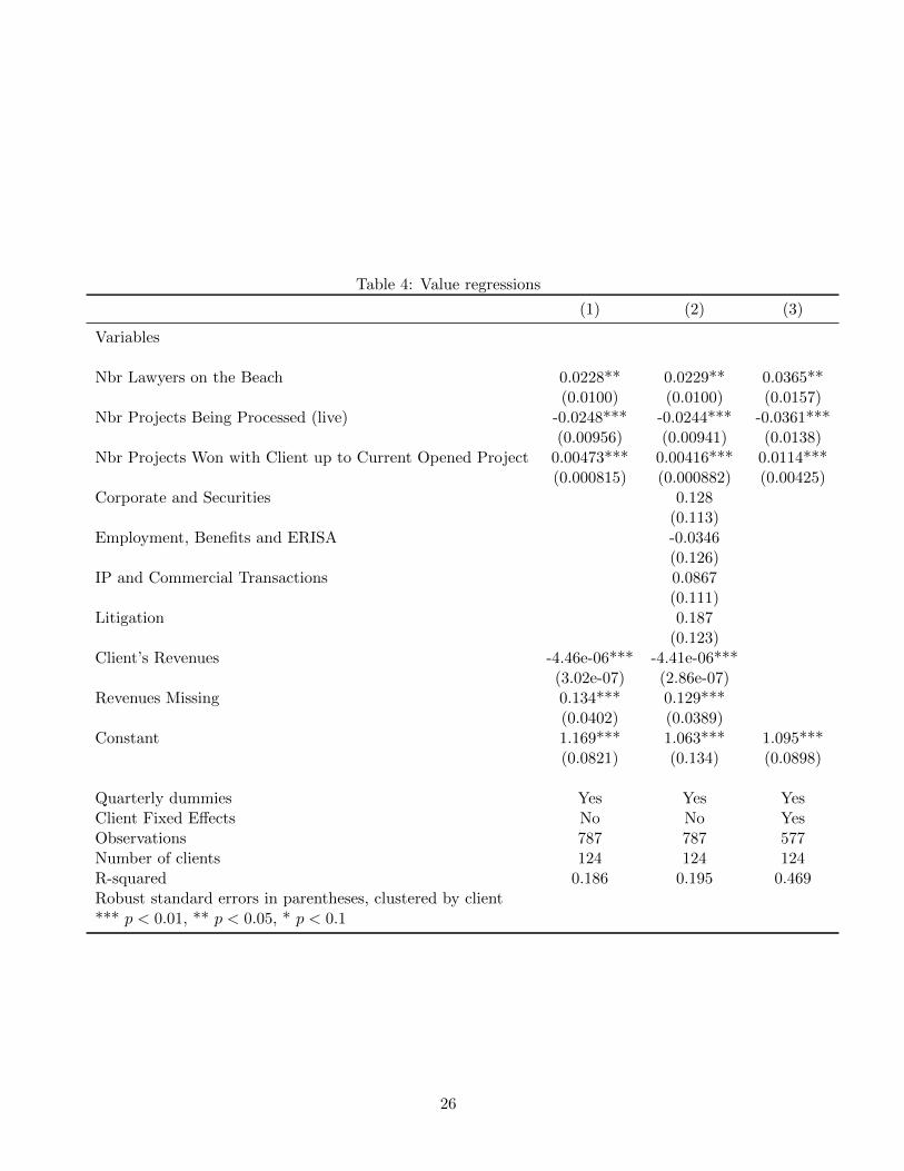
Table 4: Value regressions

(1) (2) (3)

Variables

Nbr Lawyers on the Beach 0.0228** 0.0229** 0.0365**(0.0100) (0.0100) (0.0157)

Nbr Projects Being Processed (live) -0.0248*** -0.0244*** -0.0361***(0.00956) (0.00941) (0.0138)

Nbr Projects Won with Client up to Current Opened Project 0.00473*** 0.00416*** 0.0114***(0.000815) (0.000882) (0.00425)

Corporate and Securities 0.128(0.113)

Employment, Benefits and ERISA -0.0346(0.126)

IP and Commercial Transactions 0.0867(0.111)

Litigation 0.187(0.123)

Client’s Revenues -4.46e-06*** -4.41e-06***(3.02e-07) (2.86e-07)

Revenues Missing 0.134*** 0.129***(0.0402) (0.0389)

Constant 1.169*** 1.063*** 1.095***(0.0821) (0.134) (0.0898)

Quarterly dummies Yes Yes YesClient Fixed Effects No No YesObservations 787 787 577Number of clients 124 124 124R-squared 0.186 0.195 0.469Robust standard errors in parentheses, clustered by client*** p < 0.01, ** p < 0.05, * p < 0.1

26

Table 5: Value regression with area-specific effects

Variables

Nbr Lawyers on the Beach in Corporate and Securities 0.0374**(0.0180)

Nbr Lawyers on the Beach in Benefits and ERISA 0.0264(0.0448)

Nbr Lawyers on the Beach in IP and Commercial Transactions 0.0317(0.0209)

Nbr Lawyers on the Beach in Litigation 0.0332(0.0299)

Nbr Lawyers on the Beach in Real Estate 0.0625*(0.0330)

Nbr Projects Being Processed (live) in Corporate and Securities -0.0456***(0.0147)

Nbr Projects Being Processed (live) in Benefits and ERISA -0.0446(0.0429)

Nbr Projects Being Processed (live) in IP and Commercial Transactions -0.0201(0.0163)

Nbr Projects Being Processed (live) in Litigation -0.0650**(0.0286)

Nbr Projects Being Processed (live) in Real Estate -0.00945(0.0321)

Nbr Projects Won with Client up to Current Opened Project 0.0148***(0.00412)

Corporate and Securities 0.737*(0.410)

Employment, Benefits and ERISA 0.733(0.539)

IP and Commercial Transactions 0.619(0.411)

Litigation 1.056**(0.503)

Constant 0.379(0.395)

Quarterly dummies YesClient Fixed Effects YesObservations 577Number of clients 124R-squared 0.484Robust standard errors in parentheses, clustered by client*** p < 0.01, ** p < 0.05, * p < 0.1Real Estate is the omitted category

27

Documents

Timing is Everything? An Empirical Analysis of the