Embed Size (px)
Citation preview
Timing Impairments and Clock Quality Metrics
Kishan ShenoiAnurag Gupta Kishan Shenoi
Qulsar
Anurag Gupta
Aviat Networks
WSTS – 2013, San Jose, April 16-18, 2013
Presentation Outline
� Clock Metrics in Telecommunications
� Time Error for Physical Layer Clock Signals� MTIE/MRTIE and TDEV metrics
� Physical Layer Timing Impairments� Clock Recovery Jitter (data-dependent)
� Slips in synchronous multiplexing schemes
� Bit-stuffing-induced jitter/wander
� Time Error for Packet-based Timing Signals� MATIE/MAFE, xTDEV, Floor-population-metrics, etc.
� Packet Layer Timing Impairments� Packet Delay Variation
� Asymmetry
� Beating Effects
Note: Special thanks to Stefano Ruffini of Ericsson
Clock Metrics in Telecommunications
� Time-Division Multiplexing requires synchronization� e.g. all DS1/E1 bearers must be synchronized to line-clock
� Poor synchronization results in slips (transmission errors)
� Real-time services as well as mobile technologies require
synchronization� Physical layer (SDH/SyncE) or via packets (Circuit Emulation/IEEE1588)
� Regardless of whether network is circuit-switched (TDM) or packet-switched
(IP/ATM/etc.)
� Network equipment clocks must meet specifications � Network equipment clocks must meet specifications � Clock output signal must meet prescribed MTIE and/or TDEV masks (clock
“output” may be internal to NE)
� Tolerance requirements are implied in TDM networks. Active area of study in
packet networks
� Output verification:� Obtain time interval error (TIE) sequence by comparing clock output signal
against (known) reference
� Compute TDEV, MTIE (MRTIE) from TIE data and compare against
prescribed mask
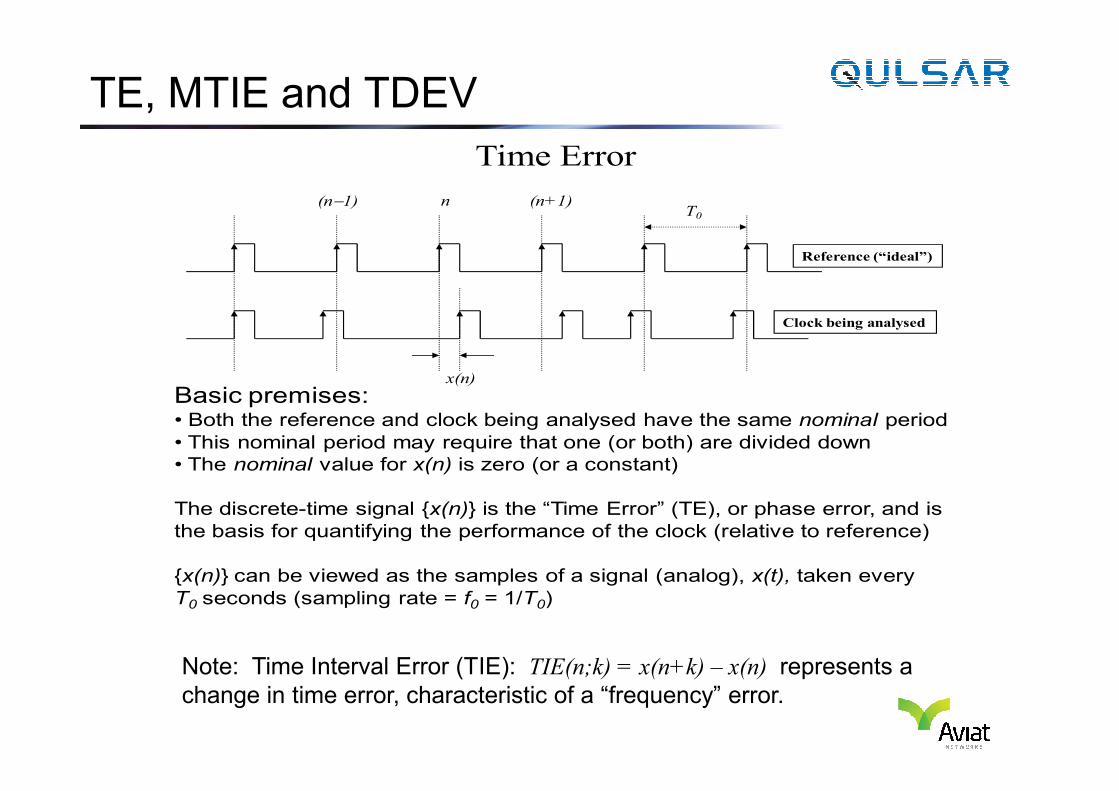
TE, MTIE and TDEV
Time Error
Reference (“ideal”)
Clock being analysed
T0
n (n+1)(n−1)
x(n)
Basic premises:Basic premises:• Both the reference and clock being analysed have the same nominal period
• This nominal period may require that one (or both) are divided down
• The nominal value for x(n) is zero (or a constant)
The discrete-time signal {x(n)} is the “Time Error” (TE), or phase error, and is
the basis for quantifying the performance of the clock (relative to reference)
{x(n)} can be viewed as the samples of a signal (analog), x(t), taken every
T0 seconds (sampling rate = f0 = 1/T0)
Note: Time Interval Error (TIE): TIE(n;k) = x(n+k) – x(n) represents a
change in time error, characteristic of a “frequency” error.
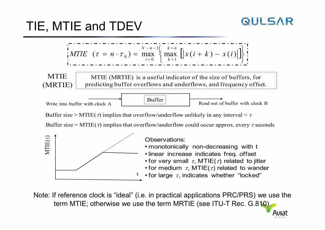
TIE, MTIE and TDEV
MTIE
(MRTIE)
MTIE (MRTIE) is a useful indicator of the size of buffers, for
predicting buffer overflows and underflows, and frequency offset.
BufferWrite into buffer with clock A Read out of buffer with clock B
Buffer size > MTIE(τ) implies that overflow/underflow unlikely in any interval < τ
[ ]
−+=⋅=
=
=
−−
=)()(maxmax)(
1
1
00 ixkixnMTIE
nk
k
nN
iττ
Buffer size > MTIE(τ) implies that overflow/underflow unlikely in any interval < τ
Buffer size = MTIE(τ) implies that overflow/underflow could occur approx. every τ seconds
τ
Observations:
• monotonically non-decreasing with t
• linear increase indicates freq. offset
• for very small τ, MTIE(τ) related to jitter
• for medium τ, MTIE(τ) related to wander
• for large τ, indicates whether “locked”
Note: If reference clock is “ideal” (i.e. in practical applications PRC/PRS) we use the
term MTIE; otherwise we use the term MRTIE (see ITU-T Rec. G.810).
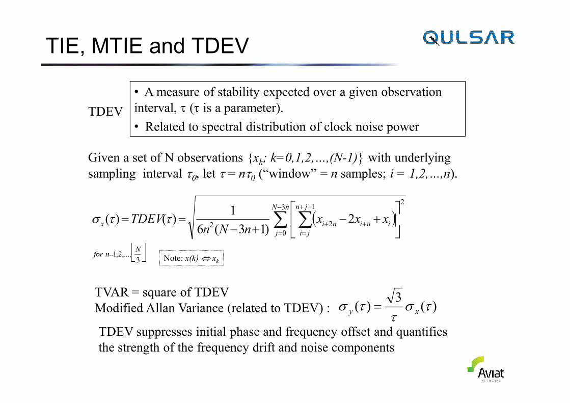
TIE, MTIE and TDEV
TDEV
• A measure of stability expected over a given observation
interval, τ (τ is a parameter).
• Related to spectral distribution of clock noise power
Given a set of N observations {xk; k=0,1,2,…,(N-1)} with underlying
sampling interval τ0, let τ = nτ0 (“window” = n samples; i = 1,2,…,n).
2−+ ( )
3,...,2,1
3
0
21
222
)13(6
1)()(
Nnfor
nN
j
jn
ji
ininix xxxnNn
TDEV
=
−
=
−+
=++∑ ∑
+−
+−== ττσ
TVAR = square of TDEV
Modified Allan Variance (related to TDEV) : )(3
)( τστ
τσ xy =
Note: x(k) ⇔ xk
TDEV suppresses initial phase and frequency offset and quantifies
the strength of the frequency drift and noise components
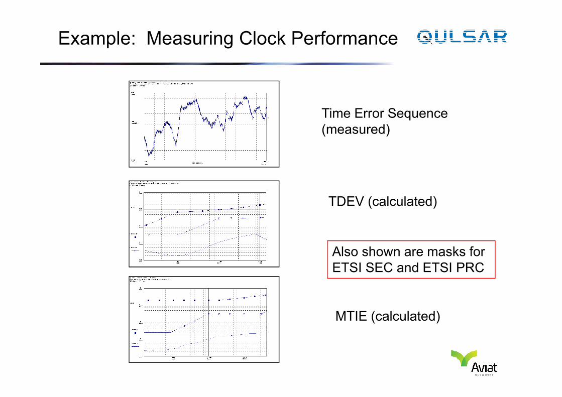
Example: Measuring Clock Performance
Time Error Sequence
(measured)
TDEV (calculated)TDEV (calculated)
MTIE (calculated)
Also shown are masks for
ETSI SEC and ETSI PRC
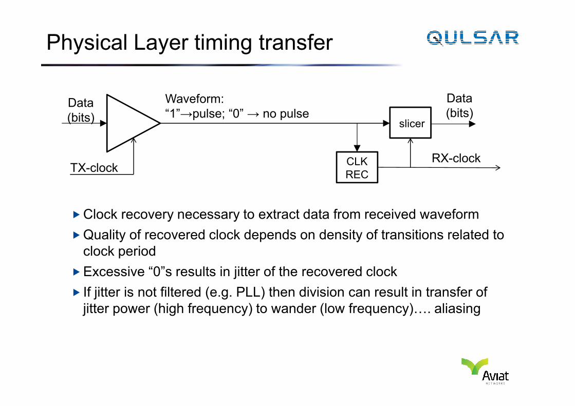
Physical Layer timing transfer
Data
(bits)
TX-clock
Waveform:
“1”→pulse; “0” → no pulseslicer
CLK
REC
RX-clock
Data
(bits)
�Clock recovery necessary to extract data from received waveform
�Quality of recovered clock depends on density of transitions related to
clock period
�Excessive “0”s results in jitter of the recovered clock
� If jitter is not filtered (e.g. PLL) then division can result in transfer of
jitter power (high frequency) to wander (low frequency)…. aliasing
time
channel clock
channel data
assembly data
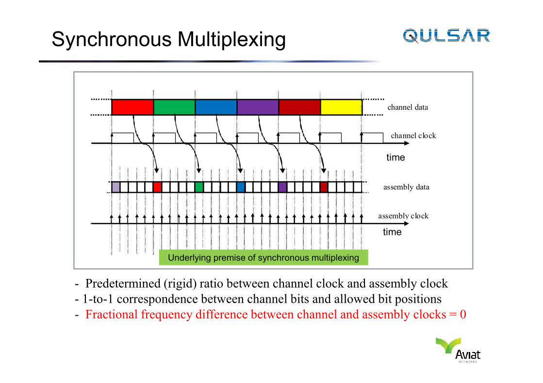
Synchronous Multiplexing
assembly clock
time
Underlying premise of synchronous multiplexing
- Predetermined (rigid) ratio between channel clock and assembly clock
- 1-to-1 correspondence between channel bits and allowed bit positions
- Fractional frequency difference between channel and assembly clocks = 0
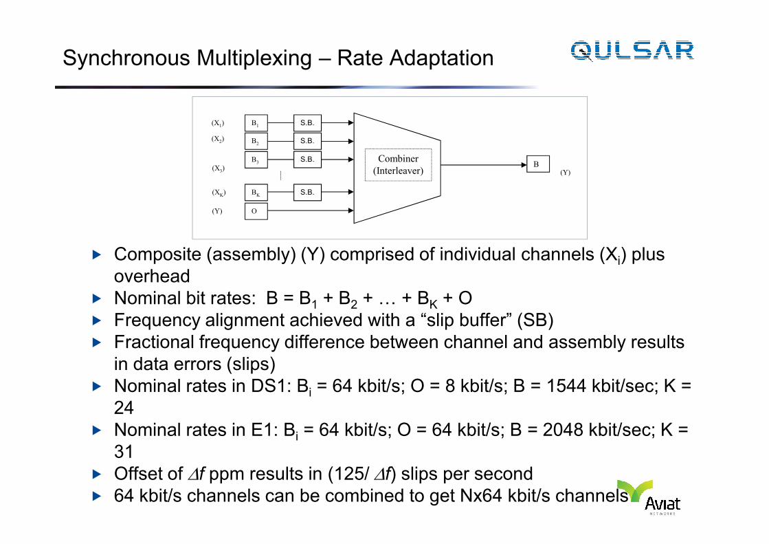
Synchronous Multiplexing – Rate Adaptation
� Composite (assembly) (Y) comprised of individual channels (Xi) plus
overhead
B2
B1
B3
BK
O
BCombiner
(Interleaver)
(X1)
(X2)
(X3)
(XK)
(Y)
(Y)
S.B.
S.B.
S.B.
S.B.
overhead
� Nominal bit rates: B = B1 + B2 + … + BK + O
� Frequency alignment achieved with a “slip buffer” (SB)
� Fractional frequency difference between channel and assembly results
in data errors (slips)
� Nominal rates in DS1: Bi = 64 kbit/s; O = 8 kbit/s; B = 1544 kbit/sec; K =
24
� Nominal rates in E1: Bi = 64 kbit/s; O = 64 kbit/s; B = 2048 kbit/sec; K =
31
� Offset of ∆f ppm results in (125/ ∆f) slips per second
� 64 kbit/s channels can be combined to get Nx64 kbit/s channels
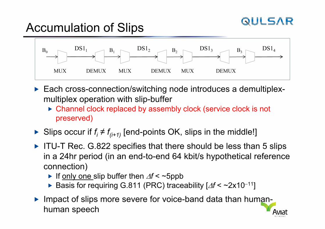
Accumulation of Slips
� Each cross-connection/switching node introduces a demultiplex-
multiplex operation with slip-buffer� Channel clock replaced by assembly clock (service clock is not
preserved)
B0DS11 B1
DS12 B2
MUX DEMUX MUX DEMUX
DS13 B3
MUX DEMUX
DS14
preserved)
� Slips occur if fi ≠ f(i+1) [end-points OK, slips in the middle!]
� ITU-T Rec. G.822 specifies that there should be less than 5 slips
in a 24hr period (in an end-to-end 64 kbit/s hypothetical reference
connection)� If only one slip buffer then ∆f < ~5ppb
� Basis for requiring G.811 (PRC) traceability [∆f < ~2x10⁻¹¹]
� Impact of slips more severe for voice-band data than human-
human speech
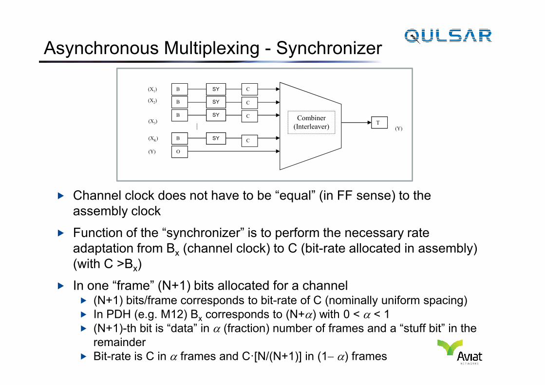
Asynchronous Multiplexing - Synchronizer
� Channel clock does not have to be “equal” (in FF sense) to the
B
B
B
B
O
TCombiner
(Interleaver)
(X1)
(X2)
(X3)
(XK)
(Y)
(Y)
SY
SY
SY
SY
C
C
C
C
� Channel clock does not have to be “equal” (in FF sense) to the
assembly clock
� Function of the “synchronizer” is to perform the necessary rate
adaptation from Bx (channel clock) to C (bit-rate allocated in assembly)
(with C >Bx)
� In one “frame” (N+1) bits allocated for a channel� (N+1) bits/frame corresponds to bit-rate of C (nominally uniform spacing)
� In PDH (e.g. M12) Bx corresponds to (N+α) with 0 < α < 1
� (N+1)-th bit is “data” in α (fraction) number of frames and a “stuff bit” in the
remainder
� Bit-rate is C in α frames and C·[N/(N+1)] in (1− α) frames
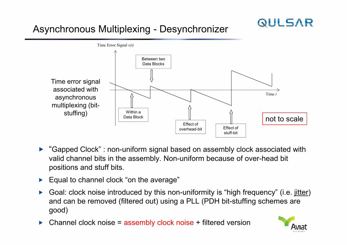
Asynchronous Multiplexing - Desynchronizer
Time Error Signal x(t)
Time t
Within a
Data Block
Between two
Data Blocks
Time error signal
associated with
asynchronous
multiplexing (bit-
stuffing)
Effect of not to scale
� “Gapped Clock” : non-uniform signal based on assembly clock associated with
valid channel bits in the assembly. Non-uniform because of over-head bit
positions and stuff bits.
� Equal to channel clock “on the average”
� Goal: clock noise introduced by this non-uniformity is “high frequency” (i.e. jitter)
and can be removed (filtered out) using a PLL (PDH bit-stuffing schemes are
good)
� Channel clock noise = assembly clock noise + filtered version
Effect of
stuff-bit
Effect of
overhead-bit
not to scale
SONET/SDH : SM & AM features
� STS-N created by interleaving N STS-1s; STM-N created by
interleaving STM-1s� STS-1s (STM-1s) must be synchronized (zero frequency offset between
constituent channels and assembly)
� Constituents channels of STS-1 are synchronous to STS1 (“containers”)
� Bearer channels encapsulated into “containers”.� e.g. VT1.5 is a container for a DS1 (1.544 Mbit/s signal)
� The synchronizer function for DS1 → VT1.5 employs “positive-zero-� The synchronizer function for DS1 → VT1.5 employs “positive-zero-
negative stuffing”
� Synchronizer function differences� PDH uses “positive stuffing”. Clock noise introduced is high-frequency
(jitter) and can be filtered out
� SONET/SDH use “positive-zero-negative” stuffing that can introduce low-
frequency (wander) components
� DS1-bearer in PDH can be used as a synchronization reference; DS1-
bearer in SONET is not used as a synchronization reference
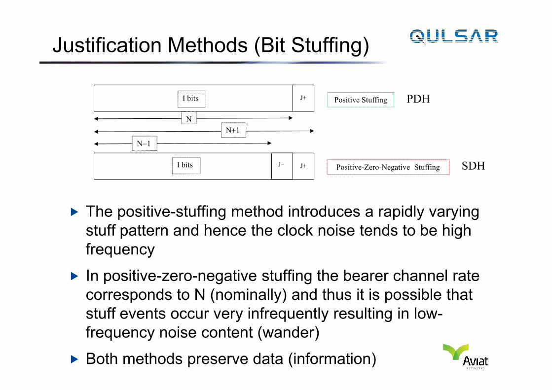
Justification Methods (Bit Stuffing)
J−
J+
J+
Positive Stuffing
N
N−1
N+1
I bits
I bits Positive-Zero-Negative Stuffing
PDH
SDH
� The positive-stuffing method introduces a rapidly varying
stuff pattern and hence the clock noise tends to be high
frequency
� In positive-zero-negative stuffing the bearer channel rate
corresponds to N (nominally) and thus it is possible that
stuff events occur very infrequently resulting in low-
frequency noise content (wander)
� Both methods preserve data (information)
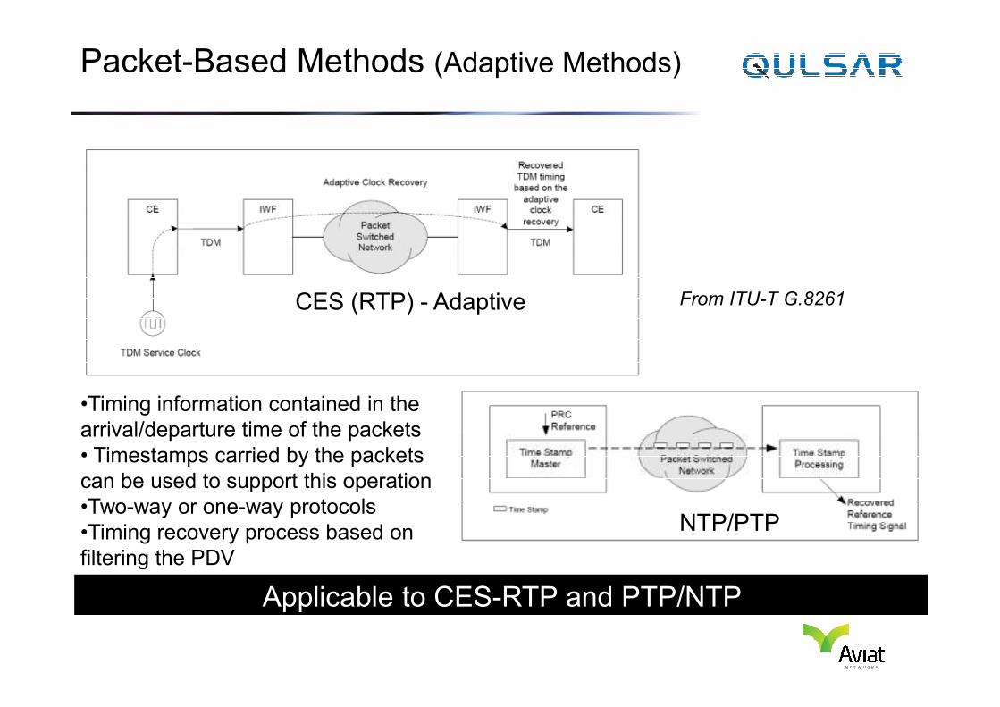
Packet-Based Methods (Adaptive Methods)
From ITU-T G.8261CES (RTP) - Adaptive
Applicable to CES-RTP and PTP/NTP
•Timing information contained in the
arrival/departure time of the packets
• Timestamps carried by the packets
can be used to support this operation
•Two-way or one-way protocols
•Timing recovery process based on
filtering the PDV
NTP/PTP
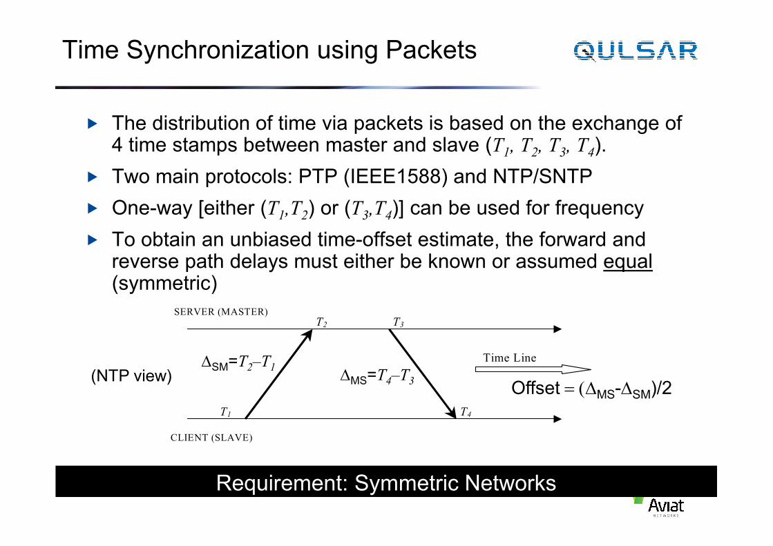
Time Synchronization using Packets
� The distribution of time via packets is based on the exchange of 4 time stamps between master and slave (T1, T2, T3, T4).
� Two main protocols: PTP (IEEE1588) and NTP/SNTP
� One-way [either (T1,T2) or (T3,T4)] can be used for frequency
� To obtain an unbiased time-offset estimate, the forward and reverse path delays must either be known or assumed equal(symmetric)(symmetric)
Time Line
CLIENT (SLAVE)
SERVER (MASTER)
T1
T2 T3
T4
∆SM=T2–T1∆MS=T4–T3
Offset = (∆MS-∆SM)/2
Requirement: Symmetric Networks
(NTP view)
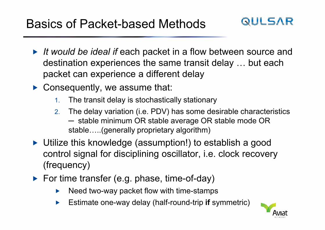
� It would be ideal if each packet in a flow between source and
destination experiences the same transit delay … but each
packet can experience a different delay
� Consequently, we assume that:
1. The transit delay is stochastically stationary
2. The delay variation (i.e. PDV) has some desirable characteristics
Basics of Packet-based Methods
2. The delay variation (i.e. PDV) has some desirable characteristics
─ stable minimum OR stable average OR stable mode OR
stable…..(generally proprietary algorithm)
� Utilize this knowledge (assumption!) to establish a good
control signal for disciplining oscillator, i.e. clock recovery
(frequency)
� For time transfer (e.g. phase, time-of-day)
� Need two-way packet flow with time-stamps
� Estimate one-way delay (half-round-trip if symmetric)
Impairments in Packet networks
� Typical Impairments in the packet networks� Packet delay variations [ PDV]
�Equipment design
�Equipment configuration
� Path dependent aspects�Physical path asymmetry
�Path rerouting �Path rerouting
� Interactions between the packet streams
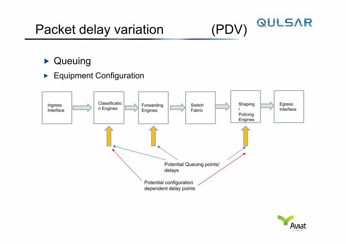
Packet delay variation (PDV)
� Queuing
� Equipment Configuration
Ingress
Interface
Classificatio
n EnginesForwarding
Engines
Switch
Fabric
Shaping
/
Policing
Engines
Egress
Interface
Potential Queuing points/
delays
Potential configuration
dependent delay points
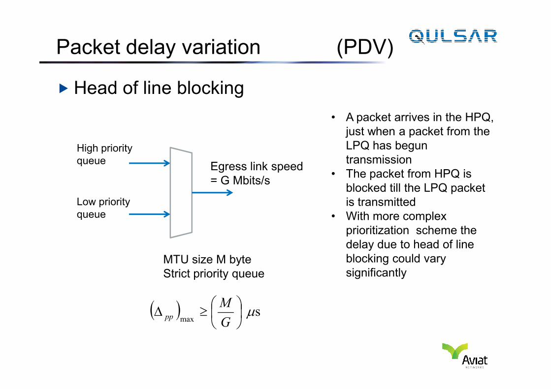
Packet delay variation (PDV)
� Head of line blocking
Egress link speed
= G Mbits/s
High priority
queue
• A packet arrives in the HPQ,
just when a packet from the
LPQ has begun
transmission
• The packet from HPQ is
blocked till the LPQ packet
MTU size M byte
Strict priority queue
Low priority
queue
( ) s max
µ
≥∆G
Mpp
is transmitted
• With more complex
prioritization scheme the
delay due to head of line
blocking could vary
significantly
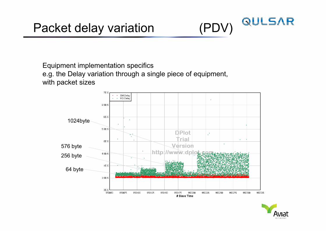
Packet delay variation (PDV)
Equipment implementation specifics
e.g. the Delay variation through a single piece of equipment,
with packet sizes
64 byte
256 byte
576 byte
1024byte
Path dependent impairments
� Asymmetry� Static Difference in paths between the forward and
reverse paths. E.g difference in lengths of fiber
� Forward and reverse paths pass through different node
� Rerouting� Leads change in path delays and can “confuse” the � Leads change in path delays and can “confuse” the
algorithms.
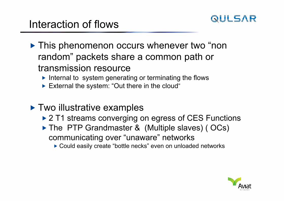
Interaction of flows
� This phenomenon occurs whenever two “non
random” packets share a common path or
transmission resource� Internal to system generating or terminating the flows
� External the system: “Out there in the cloud”
� Two illustrative examples� 2 T1 streams converging on egress of CES Functions
� The PTP Grandmaster & (Multiple slaves) ( OCs)
communicating over “unaware” networks� Could easily create “bottle necks” even on unloaded networks
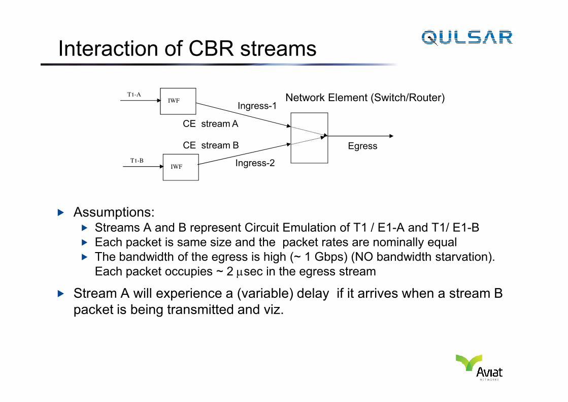
Interaction of CBR streams
CE stream A
CE stream B
Ingress-1
Ingress-2
Egress
Network Element (Switch/Router)T1-AIWF
T1-BIWF
� Assumptions:� Streams A and B represent Circuit Emulation of T1 / E1-A and T1/ E1-B
� Each packet is same size and the packet rates are nominally equal
� The bandwidth of the egress is high (~ 1 Gbps) (NO bandwidth starvation).
Each packet occupies ~ 2 µsec in the egress stream
� Stream A will experience a (variable) delay if it arrives when a stream B
packet is being transmitted and viz.
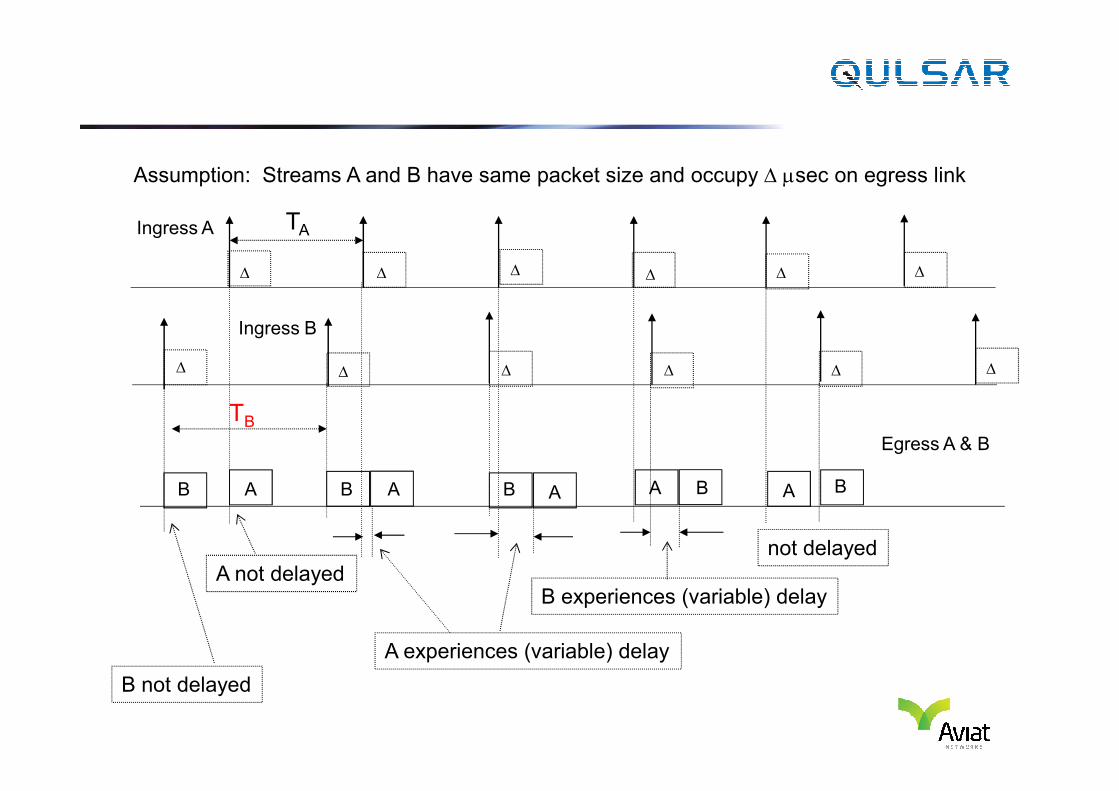
Assumption: Streams A and B have same packet size and occupy ∆ µsec on egress link
∆ ∆ ∆
∆ ∆ ∆ ∆
∆
∆
∆
∆
∆
TAIngress A
Ingress B
B A B A B A A B A B
B not delayed
A not delayed
A experiences (variable) delay
B experiences (variable) delay
not delayed
TB
Egress A & B
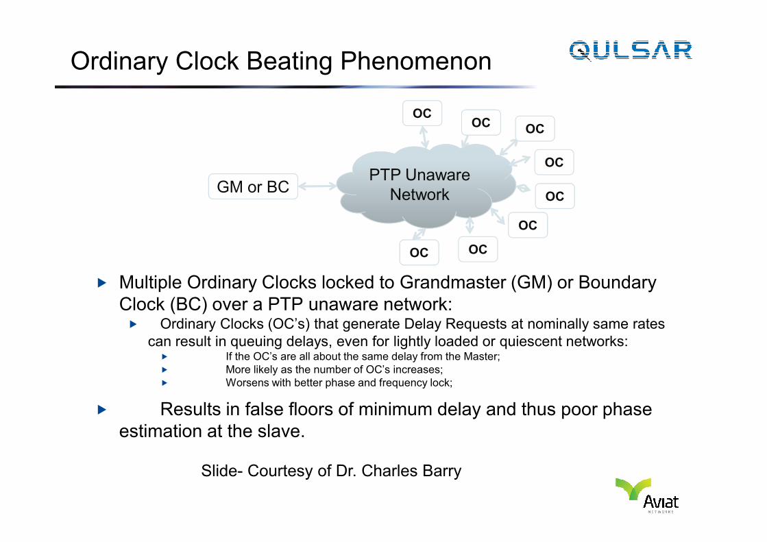
Ordinary Clock Beating Phenomenon
PTP Unaware
NetworkGM or BC
OC
OC
OC
OC
OC
OCOC
OC
� Multiple Ordinary Clocks locked to Grandmaster (GM) or Boundary
Clock (BC) over a PTP unaware network:� Ordinary Clocks (OC’s) that generate Delay Requests at nominally same rates
can result in queuing delays, even for lightly loaded or quiescent networks:� If the OC’s are all about the same delay from the Master;
� More likely as the number of OC’s increases;
� Worsens with better phase and frequency lock;
� Results in false floors of minimum delay and thus poor phase
estimation at the slave.
Slide- Courtesy of Dr. Charles Barry
Ordinary Clock Beating Phenomenon
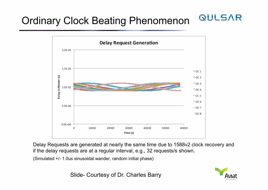
Delay Requests are generated at nearly the same time due to 1588v2 clock recovery and
if the delay requests are at a regular interval, e.g., 32 requests/s shown.
(Simulated +/- 1.0us sinusoidal wander, random initial phase)
Slide- Courtesy of Dr. Charles Barry
Ordinary Clock Beating Phenomenon
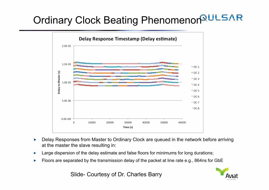
� Delay Responses from Master to Ordinary Clock are queued in the network before arriving
at the master the slave resulting in:
� Large dispersion of the delay estimate and false floors for minimums for long durations;
� Floors are separated by the transmission delay of the packet at line rate e.g., 864ns for GbE
Slide- Courtesy of Dr. Charles Barry
Ordinary Clock Beating Phenomenon
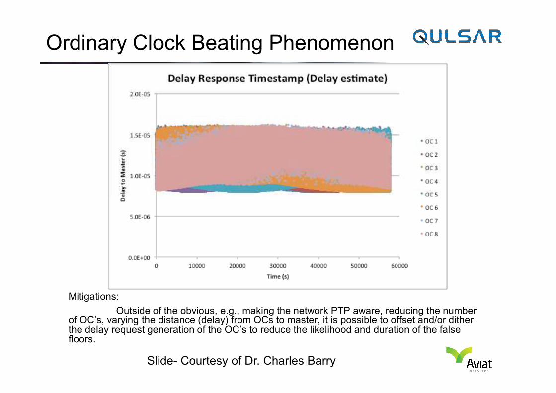
Mitigations:
Outside of the obvious, e.g., making the network PTP aware, reducing the number of OC’s, varying the distance (delay) from OCs to master, it is possible to offset and/or dither the delay request generation of the OC’s to reduce the likelihood and duration of the false floors.
Slide- Courtesy of Dr. Charles Barry
Key Aspects of Performance
� Packet Delay Variation (PDV) is a major contributor to “clock
noise”� Related to number of hops, congestion, line-bit-rate, queuing
priority, etc. Time-stamp-error can be viewed as part of PDV
� Clock recovery involves low-pass-filter action on PDV� Oscillator characteristics determine degree of filtering capability (i.e.
tolerance to PDV)tolerance to PDV)� Higher performance oscillators allow for longer time-constants
(narrower bandwidth == stronger filtering)
� Lower performance (less expensive) oscillators may be used (may
require algorithmic performance improvements)
� Performance improvements can be achieved by� Higher packet rate
� Controlling PDV in network (e.g. network engineering, QoS)
� Timing support from network (e.g. boundary clocks in PTP)
� Packet selection and/or nonlinear processing
Sync Metrics in Packet Networks
� Depending on the application the Network element clock output metrics
(computed from TIE measurements) can be the same (MTIE/MRTIE/TDEV)
� Clock output requirements are determined by existing masks
� Some distinctions are required in case of packet clock integrated in
the Base Station (no standardized output MTIE/TDEV)
� Metrics are needed to better characterize the behavior of packet networks
(PDV) delivering the timing reference
� E.g. a metrics that could associate PDV with FFO or phase variation� E.g. a metrics that could associate PDV with FFO or phase variation
� Tolerance masks will be useful for network operators and clock
manufacturers
� Packet selection methods can be justified
� No one single “magic” metric exists� May need to have a collection of metrics
� All metrics are “useful” … a metric simply provides a quantitative
description of some property of the PDV
Need for additional metrics
� Traditional IP networks utilize just peak-to-peak “jitter” as the sole
time/timing related performance metric (e.g. 95% of delay variation samples
<10 ms)
� This is generally not sufficient for the purpose of timing recovery as is seen
in the following examples.� In all cases the synthetic PDV sequence has a peak-to-peak measure of
approximately 10ms and packet rate of 10Hz
� The PDV, pdf, and TDEV/minTDEV are shown in the following charts� The PDV, pdf, and TDEV/minTDEV are shown in the following charts
� One TDEV mask (ETSI SEC) is shown in the charts to provide a frame of
reference
� Exception: Stable oscillator (e.g. Stratum 2) and only frequency required
� Timing is generally recovered using selected “best” packets; this is not
visible in the peak-to-peak measurements� Other variations include metrics derived from the distribution of the packet-arrival times
(e.g. Mode, median, etc.)
� Suitable metric sets must include those that characterize amplitude
distribution (including peak-to-peak) and spectral distribution.
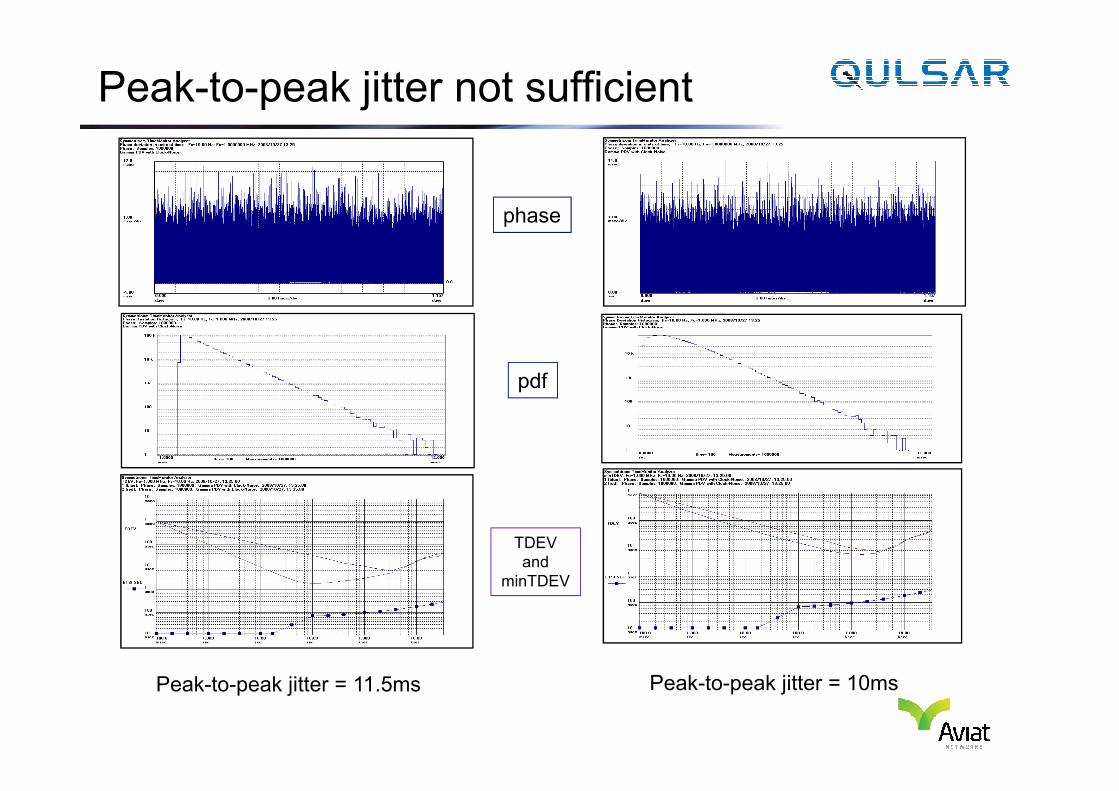
Peak-to-peak jitter not sufficient
phase
Peak-to-peak jitter = 11.5ms Peak-to-peak jitter = 10ms
TDEV
and
minTDEV
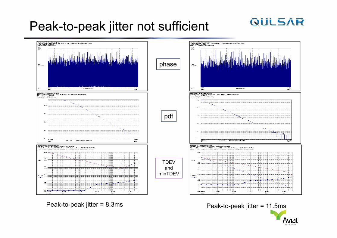
Peak-to-peak jitter not sufficient
phase
Peak-to-peak jitter = 8.3ms Peak-to-peak jitter = 11.5ms
TDEV
and
minTDEV

Thank You!
Questions?
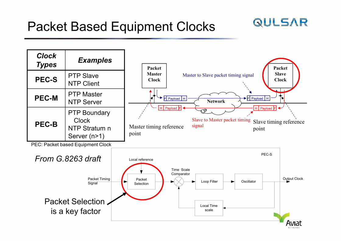
Packet Based Equipment Clocks
Payload HF
Packet
Master
Clock
Packet
Slave
Clock
NetworkPayload HF
PayloadH F PayloadH F
Master to Slave packet timing signal
Slave to Master packet timing Slave timing reference
Clock
TypesExamples
PEC-SPTP Slave
NTP Client
PEC-MPTP Master
NTP Server
PEC-B
PTP Boundary
ClockMaster timing reference
point
Slave to Master packet timing
signalSlave timing reference
point
From G.8263 draft
Packet Selection
is a key factor
Loop Filter Oscillator
Local Time
scale
Output Clock Packet Timing
SignalPacket
Selection
Local reference
Time Scale
Comparator
PEC-S
PEC-BClock
NTP Stratum n
Server (n>1)
PEC: Packet based Equipment Clock
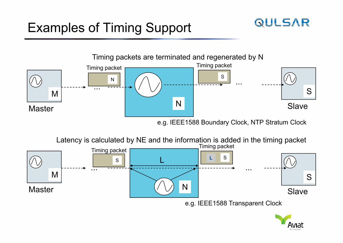
Examples of Timing Support
Timing packets are terminated and regenerated by N
N
NS
...
SM...
e.g. IEEE1588 Boundary Clock, NTP Stratum Clock
Master Slave
Timing packetTiming packet
e.g. IEEE1588 Boundary Clock, NTP Stratum Clock
Timing packetTiming packet
Latency is calculated by NE and the information is added in the timing packet
N
SS
...
S
LL...
M
e.g. IEEE1588 Transparent Clock
Master Slave
General requirements for packet-based metrics
� The basic parameter is the packet delay variation (PDV)
� ITU-T Rec. Y.1540 provides definitions for packet delay
variation
� Some processing of the PDV data is needed to get a � Some processing of the PDV data is needed to get a
proper interpretation of the packet network behaviour
(metrics)
� Different metrics may be defined and these may have
some relationship with hypothetical clock-recovery
algorithms (e.g. packet selection)
General requirements for packet-based metrics (contd)
� Requirements for the (network) metrics include: � Measurable
� Characterize real (typical) packet networks behaviour
� it shall be possible to state (e.g. 99% of the time) that “if
network meets mask A then a type X clock can meet some
defined output timing mask B”
� It should be possible to design packet networks and clocks � It should be possible to design packet networks and clocks
that can fulfill these masks
� Metric is likely to be some form of statistical average (e.g. a
variation of TDEV)
xTDEV
OK (Clock X is able to recover
Timing according to requirements)
NOK (Clock X may not be able to recover
Timing according to requrements)
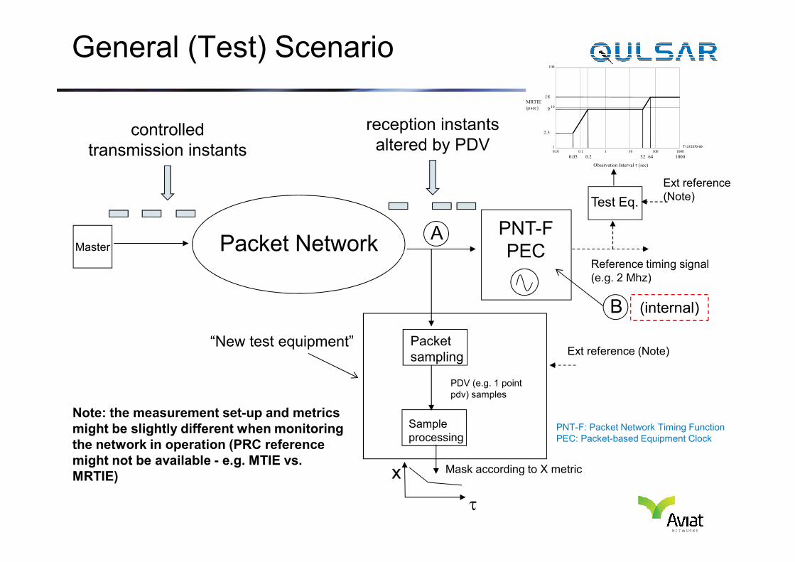
General (Test) Scenario
PNT-F
PECPacket Network
T1315370-99
Observation Interval τ (sec)
MRTIE
(µsec)
100
18
109
2.3
1
0.1 1 10 100 1000
0.05 0.2 32 64 1000
0.01
Master
Test Eq.
Ext reference
(Note)
Reference timing signal
(e.g. 2 Mhz)
controlled
transmission instants
reception instants
altered by PDV
A
PDV (e.g. 1 point
pdv) samples
Mask according to X metric
“New test equipment”Ext reference (Note)
Packet
sampling
Sample
processing
(e.g. 2 Mhz)
Note: the measurement set-up and metrics
might be slightly different when monitoring
the network in operation (PRC reference
might not be available - e.g. MTIE vs.
MRTIE) x
τ
PNT-F: Packet Network Timing Function
PEC: Packet-based Equipment Clock
B (internal)
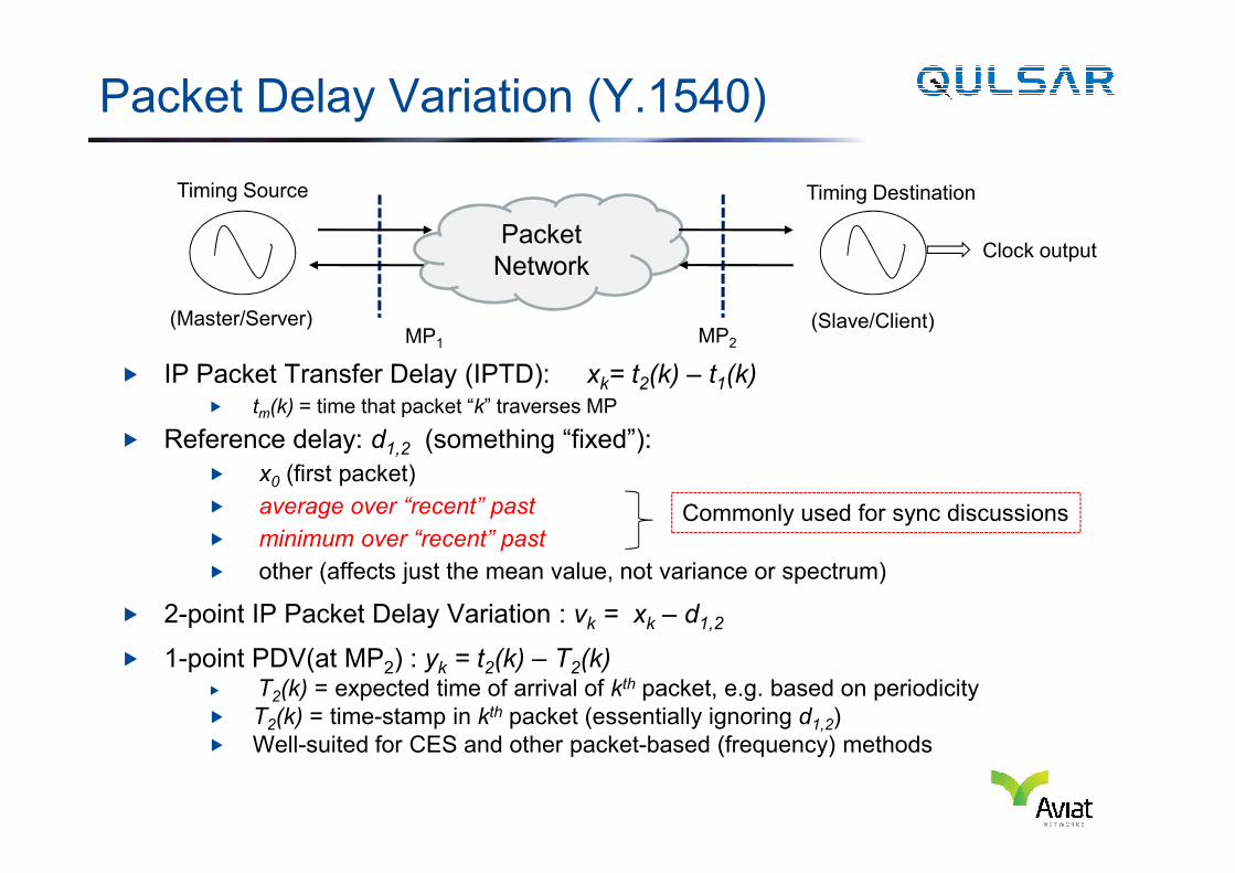
Packet Delay Variation (Y.1540)
� IP Packet Transfer Delay (IPTD): xk= t2(k) – t1(k)� tm(k) = time that packet “k” traverses MP
� Reference delay: d (something “fixed”):
Packet
Network
MP1 MP2
Timing Source Timing Destination
Clock output
(Master/Server) (Slave/Client)
� Reference delay: d1,2 (something “fixed”):
� x0 (first packet)
� average over “recent” past
� minimum over “recent” past
� other (affects just the mean value, not variance or spectrum)
� 2-point IP Packet Delay Variation : vk = xk – d1,2
� 1-point PDV(at MP2) : yk = t2(k) – T2(k) � T2(k) = expected time of arrival of kth packet, e.g. based on periodicity
� T2(k) = time-stamp in kth packet (essentially ignoring d1,2)
� Well-suited for CES and other packet-based (frequency) methods
Commonly used for sync discussions
Y.1540 and IEEE1588 in G.826x
� The Time Error (“x”) in the packet timing context� 1–point PDV as per Y.1540 in case of periodic packets (e.g. CES)
� extended definition of the 1-point PDV in case of (non-necessarily
periodic) packet timing signal carrying timestamps (e.g. time error
calculated comparing the timestamp of the packet with a reference
time generated at the output of the packet network) .
� Alternatively a modified definition of the 2-Point PDV could be used. � Alternatively a modified definition of the 2-Point PDV could be used.
� The required accuracy of the reference time in case of non-
synchronized clock configurations is under study.
� The definition of time-instant for establishing time-of-arrival
and time-of-departure of packets based on the Event
message timestamp point as defined in IEEE1588� the above definition is specified for PTP packets but could be used
for other packet protocols unless other definitions are specifically
specified.
Additional Metrics
� Several metrics addressing distribution of timing are being studied and
planned to be included in ITU-T Recc. G.8260. � minTDEV and MATIE are considered to illustrate fundamental principles
� minTDEV and percentileTDEV are analogous to TDEV� TDEV utilizes the average over windows
� minTDEV utilizes the minimum over windows
� percentileTDEV utilizes the average over the x% least delay packets
� Computed at “A” (and/or “B”)� Computed at “A” (and/or “B”)
� MATIE is related to MTIE� MTIE computed directly on the time error sequences {xk} or {yk} is not that
meaningful because of large “jitter” (PDV)
� MATIE is computed on the sequence following the pre-filtering (packet-
selection) and emulates the low-pass nature of the traditional clock model
(bandwidth / time-constant). MAFE is a variation of MATIE
� Computed at “B” (input to PLL function)
� When the application involves distribution of time-of-day, additional metrics
for quantifying network asymmetry are needed
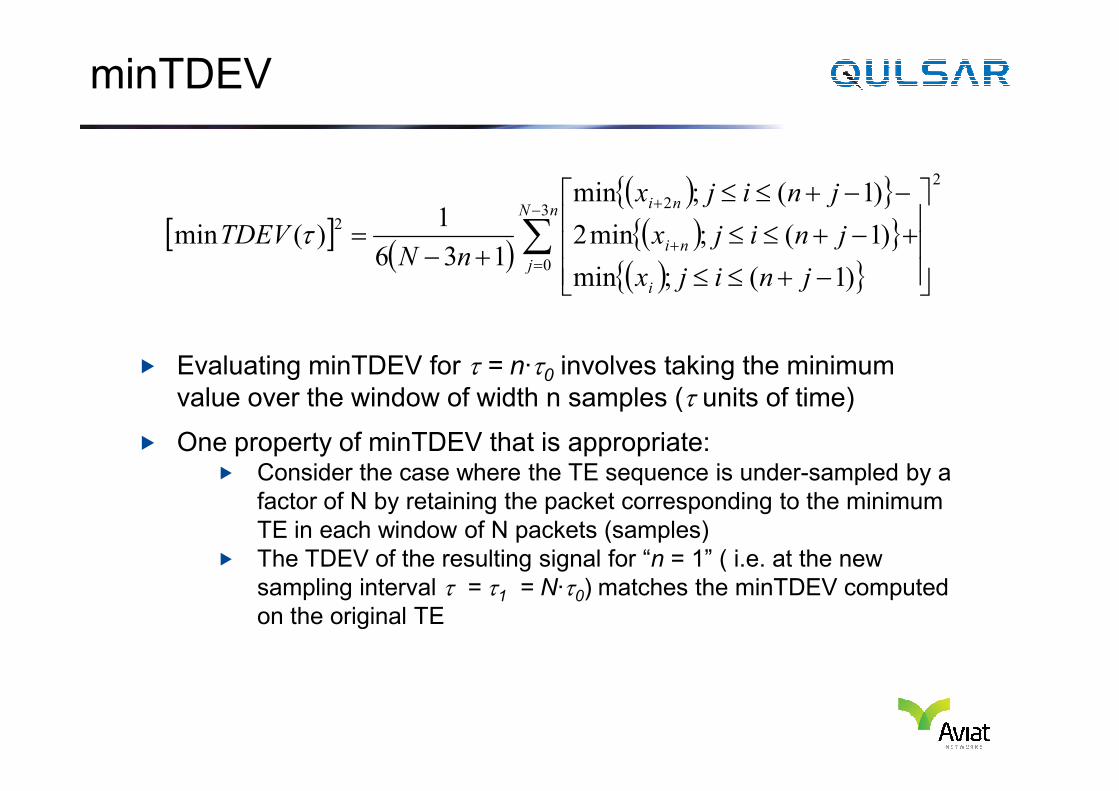
minTDEV
� Evaluating minTDEV for τ = n∙τ0 involves taking the minimum
value over the window of width n samples (τ units of time)
[ ]( )
( ){ }( ){ }
( ){ }∑
−
=+
+
−+≤≤
+−+≤≤
−−+≤≤
+−=
nN
j
i
ni
ni
jnijx
jnijx
jnijx
nNTDEV
3
0
2
2
2
)1(;min
)1(;min2
)1(;min
136
1)(min τ
value over the window of width n samples (τ units of time)
� One property of minTDEV that is appropriate:� Consider the case where the TE sequence is under-sampled by a
factor of N by retaining the packet corresponding to the minimum
TE in each window of N packets (samples)
� The TDEV of the resulting signal for “n = 1” ( i.e. at the new
sampling interval τ = τ1 = N∙τ0) matches the minTDEV computed
on the original TE
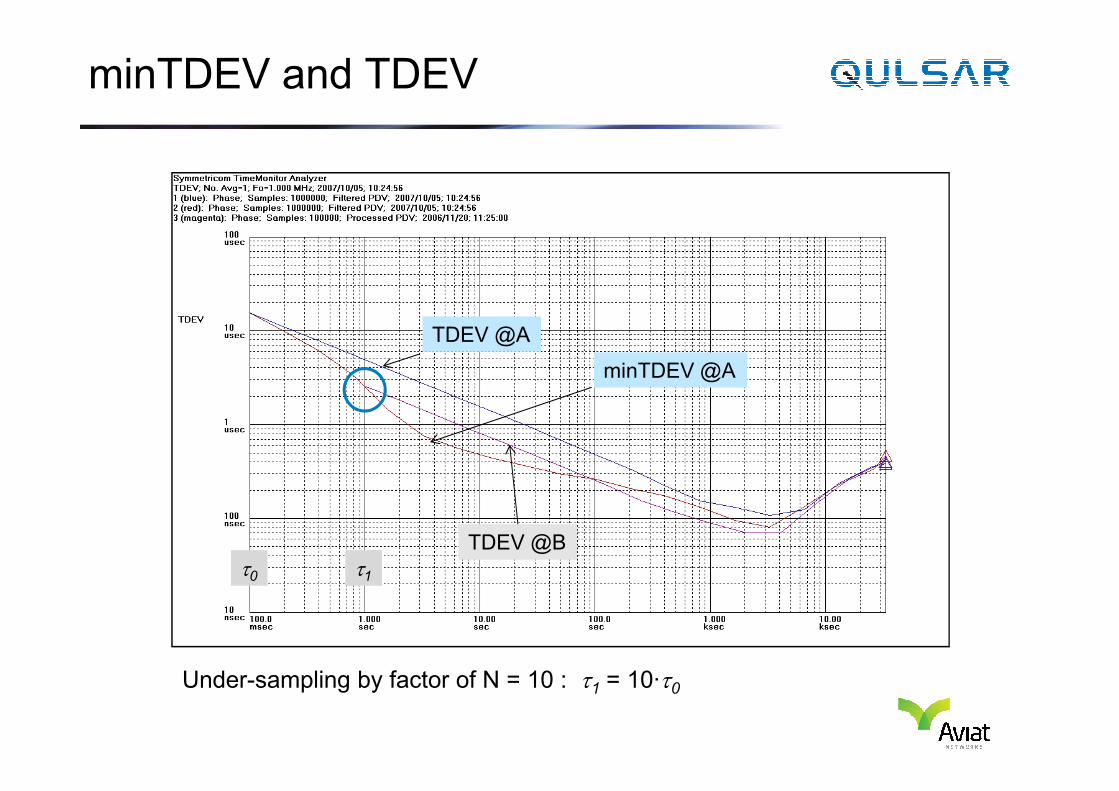
minTDEV and TDEV
TDEV @A
minTDEV @A
TDEV @B
Under-sampling by factor of N = 10 : τ1 = 10∙τ0
τ0 τ1
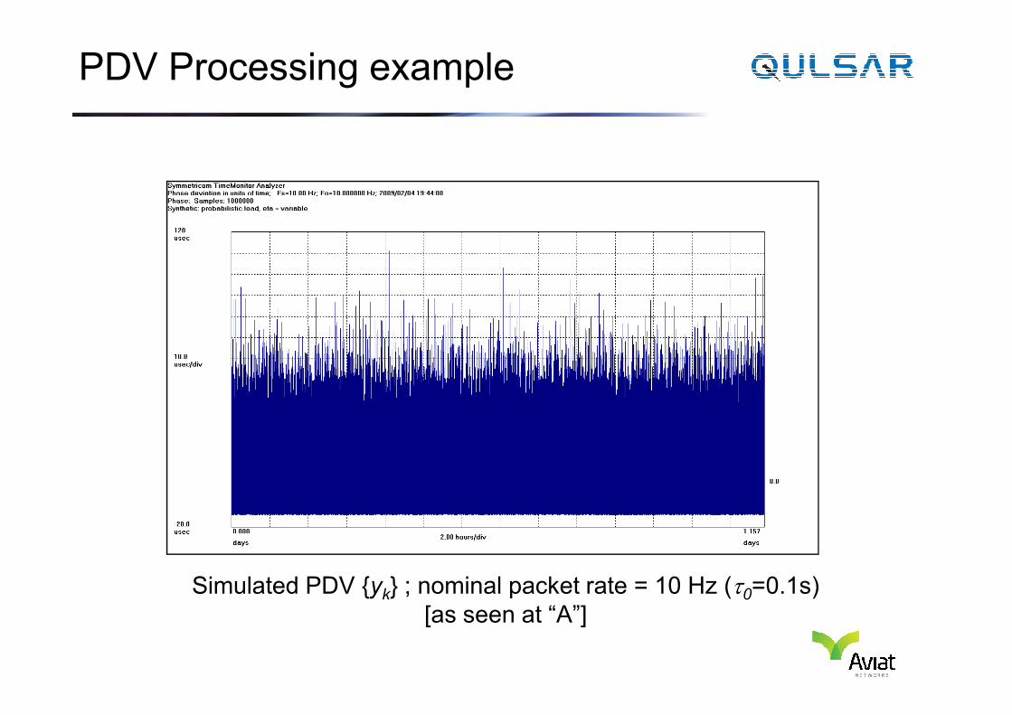
PDV Processing example
Simulated PDV {yk} ; nominal packet rate = 10 Hz (τ0=0.1s)
[as seen at “A”]
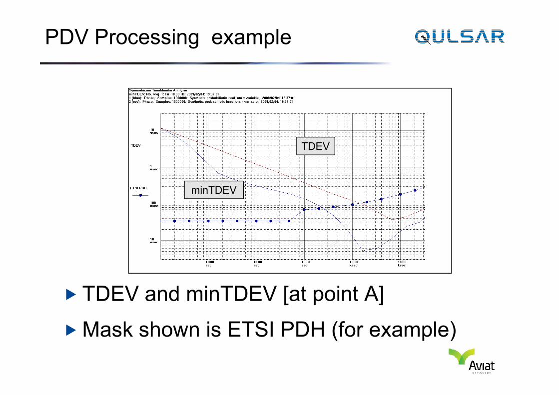
PDV Processing example
TDEV
minTDEV
� TDEV and minTDEV [at point A]
� Mask shown is ETSI PDH (for example)
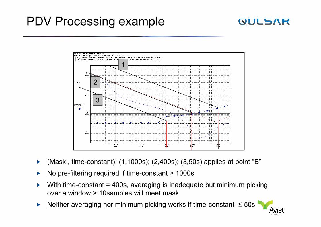
PDV Processing example
1
2
3
� (Mask , time-constant): (1,1000s); (2,400s); (3,50s) applies at point “B”
� No pre-filtering required if time-constant > 1000s
� With time-constant = 400s, averaging is inadequate but minimum picking
over a window > 10samples will meet mask
� Neither averaging nor minimum picking works if time-constant ≤ 50s
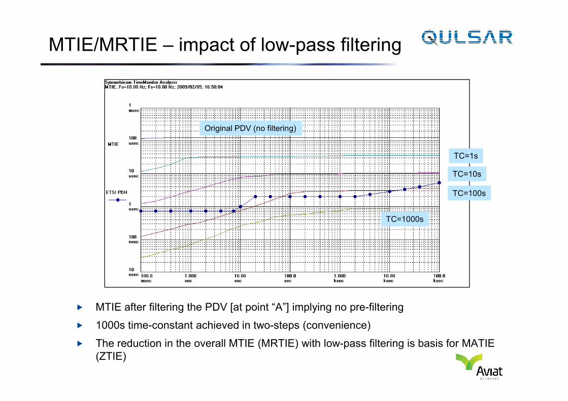
MTIE/MRTIE – impact of low-pass filtering
Original PDV (no filtering)
TC=1s
TC=10s
TC=100s
� MTIE after filtering the PDV [at point “A”] implying no pre-filtering
� 1000s time-constant achieved in two-steps (convenience)
� The reduction in the overall MTIE (MRTIE) with low-pass filtering is basis for MATIE
(ZTIE)
TC=1000s

MATIE (ZTIE) and MAFE
� Generally applied at point “B” (simulate packet selection if
necessary) where sampling interval = Ta
� Can be viewed an a bank of low-pass filters with varying
time-constant (“observation interval”)� HN(z) = (1/N)(1 + z−1 + z−2 + … +z− (N−1))
� Utilizes the notion of MTIE being a (maximum) peak-to-� Utilizes the notion of MTIE being a (maximum) peak-to-
peak measure
� MAFE(τ) = MATIE(τ)/τ
{y(nTa)}
HN(z) (1 – z−N) ABS MAX
(repeat with N = 1, 2, 3, …); τ = N∙Ta
M(N∙Ta)
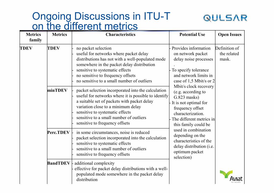
Ongoing Discussions in ITU-T on the different metrics
Metrics
family
Metrics Characteristics Potential Use Open Issues
TDEV TDEV - no packet selection
- useful for networks where packet delay
distributions has not with a well-populated mode
somewhere in the packet delay distribution
- sensitive to systematic effects
- no sensitive to frequency offsets
- no sensitive to a small number of outliers
- Provides information
on network packet
delay noise processes
.
- To specify tolerance
and network limits in
case of 1,5 Mbit/s or 2
Mbit/s clock recovery
(e.g. according to
G.823 masks)
Definition of
the related
mask.
minTDEV - packet selection incorporated into the calculation
- useful for networks where it is possible to identify G.823 masks)
- It is not optimal for
frequency offset
characterization.
- The different metrics in
this family could be
used in combination
depending on the
characteristics of the
delay distribution (i.e.
optimum packet
selection)
- useful for networks where it is possible to identify
a suitable set of packets with packet delay
variation close to a minimum delay
- sensitive to systematic effects
- sensitive to a small number of outliers
- sensitive to frequency offsets
Perc.TDEV - in some circumstances, noise is reduced
- packet selection incorporated into the calculation
- sensitive to systematic effects
- sensitive to a small number of outliers
- sensitive to frequency offsets
BandTDEV - additional complexity
- effective for packet delay distributions with a well-
populated mode somewhere in the packet delay
distribution
Ongoing Discussions in ITU-T on the different metrics, cntd
Metrics
family
Metrics Characteristics Potential Use Open Issues
MTIE MATIE -packet selection pre-processing prior
to the calculation
-predicts the performance of a first
order filter
- optimal for frequency offset
characterization in the time
domain.
- not suited for the study of noise
processes
Packet Selection
mechanism still
unclear.
Definition of the
related mask
(only corner
frequency is
relevant?).
MAFE (min
Selection)
-packet selection pre-processing prior
to the calculation
-predicts the performance of a first
order filter
- optimal for frequency offset
characterization in the frequency
domain.
- not suited for the study of noise relevant?).order filter
-sensitive to a small number of low-
lying outlier
- not suited for the study of noise
processes
- The different packet selection
approaches could be used in
combination depending on the
characteristics of the delay
distribution
MAFE (band
selection)
-packet selection pre-processing prior
to the calculation
-additional complexity
-effective for packet delay distributions
with a well-populated mode
somewhere in the packet delay
distribution
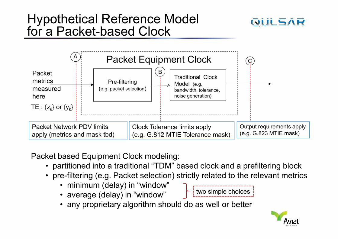
Hypothetical Reference Model for a Packet-based Clock
Traditional Clock
Model (e.g.
bandwidth, tolerance,
noise generation)
Packet Equipment Clock
Pre-filtering
(e.g. packet selection)
Packet
metrics
measured
here
TE : {xk} or {yk}
A
B
C
Output requirements apply
(e.g. G.823 MTIE mask)Clock Tolerance limits apply
(e.g. G.812 MTIE Tolerance mask)
Packet Network PDV limits
apply (metrics and mask tbd)
Packet based Equipment Clock modeling:
• partitioned into a traditional “TDM” based clock and a prefiltering block
• pre-filtering (e.g. Packet selection) strictly related to the relevant metrics
• minimum (delay) in “window”
• average (delay) in “window”
• any proprietary algorithm should do as well or better
two simple choices
PDV Metrics and Packet Based Clocks
� The definition of Packet Based Clock is a priority item in standardization bodies (e.g. ITU-T SG15/Q13 – G.8263) (see slide 11).
� Despite some clear differences with the clock traditionally used in TDM networks, there are important similarities
� The approach currently agreed upon is to model the clock with a pre-filtering function (i.e. packet selection function).
� With this model the PDV metric (mask) would apply at the input of the pre-filtering (in case of the MAFE some selection mechanism shall be assumed))assumed))
� If (traditional) MTIE/TDEV masks can be defined at the output of the pre-filtering, the remaining part of the clock can be defined according to the traditional (TDM-style) specifications
� New masks (extensions of existing masks) may be required (e.g. in case of packet based clock integrated in a Base Station there is no MTIE mask currently standardized; requirements on the radio interface is only specified in terms of frequency, e.g. 50 ppb)
� The following experiments provide justification that multiple metrics might be needed in combination...
� i.e. even if one metric provides a negative indication, it might still be OK!
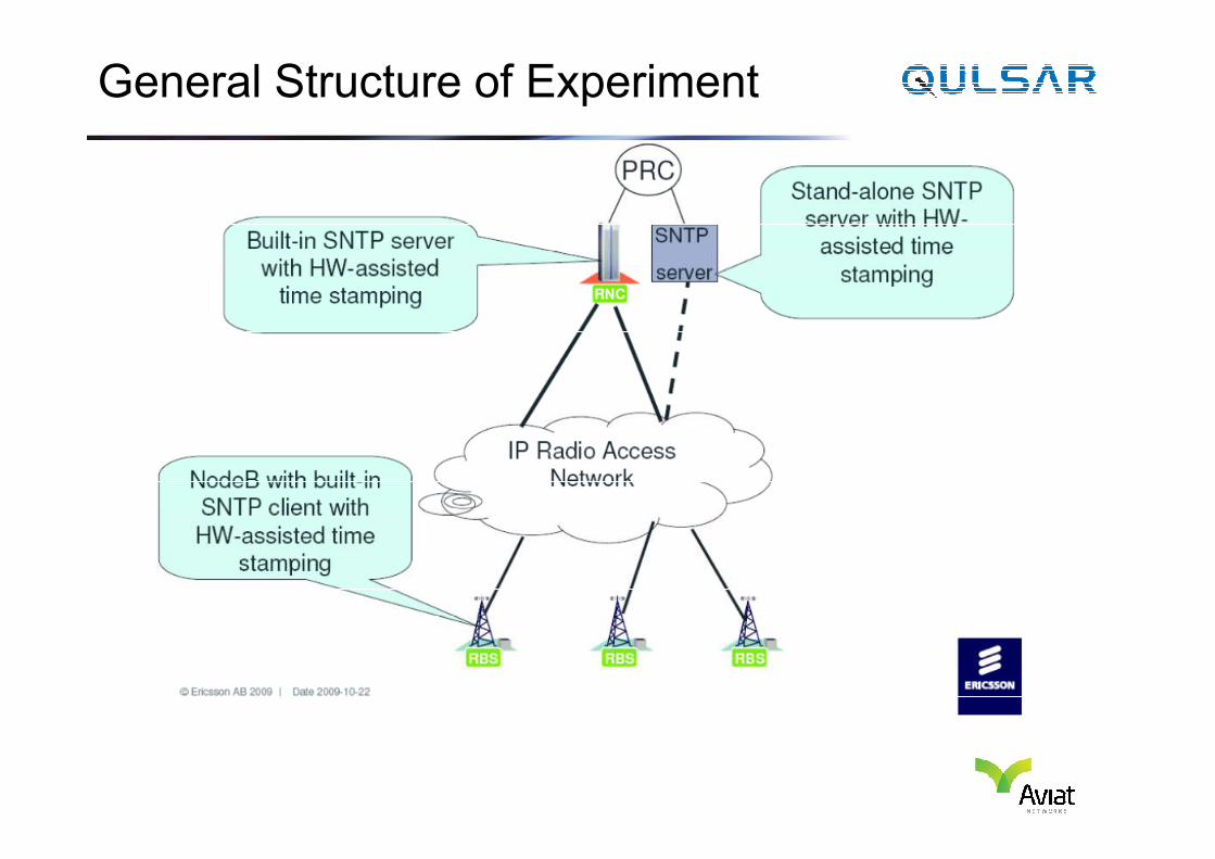
General Structure of Experiment
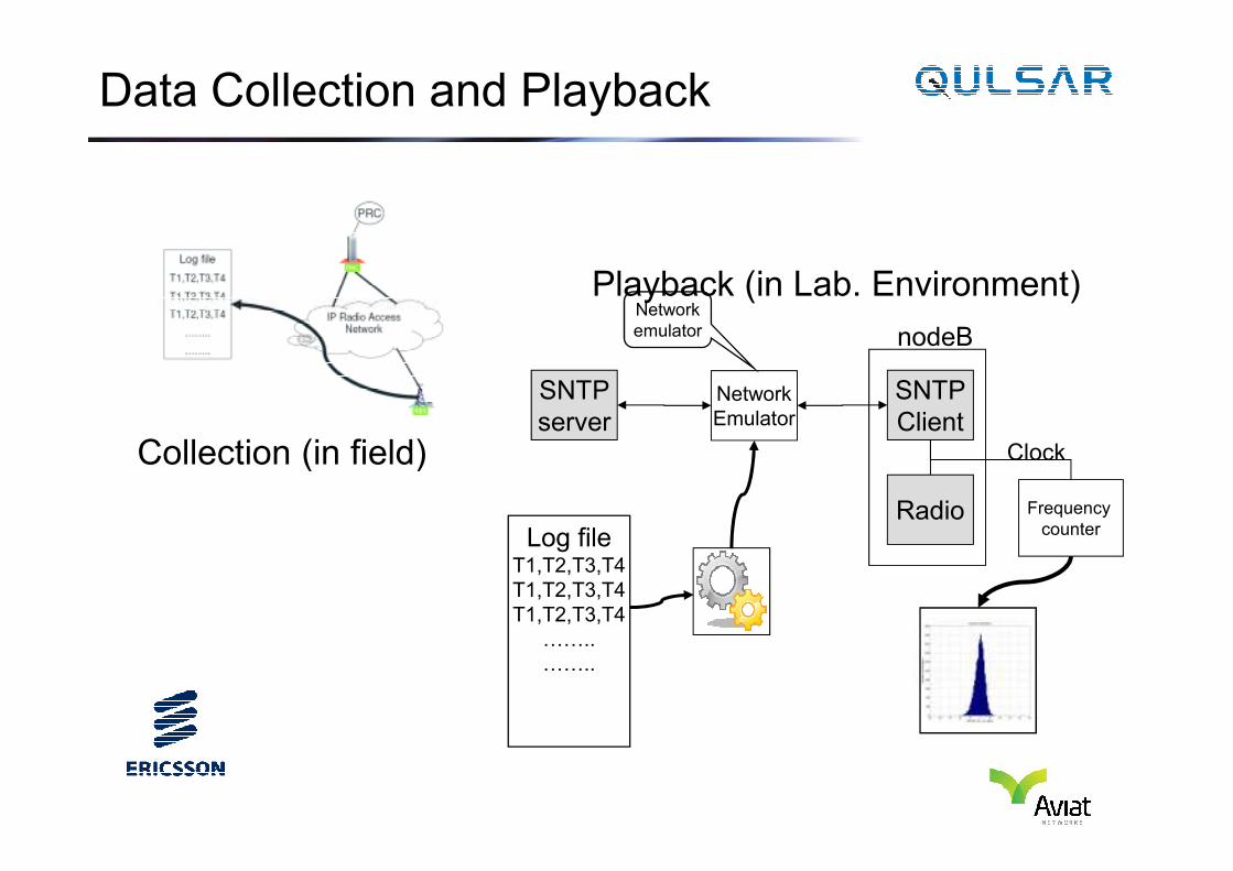
Data Collection and Playback
Collection (in field)
Playback (in Lab. Environment)
SNTP
serverNetwork
Emulator
nodeB
SNTP
Client
Network
emulator
Collection (in field)server
Radio
Client
Frequency
counter
Clock
Log fileT1,T2,T3,T4
T1,T2,T3,T4
T1,T2,T3,T4
……..
……..
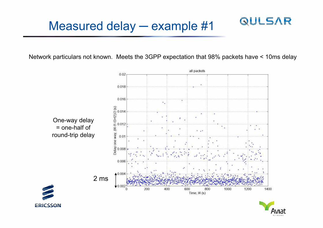
Measured delay ─ example #1
Network particulars not known. Meets the 3GPP expectation that 98% packets have < 10ms delay
One-way delay
= one-half of
round-trip delay
2 ms
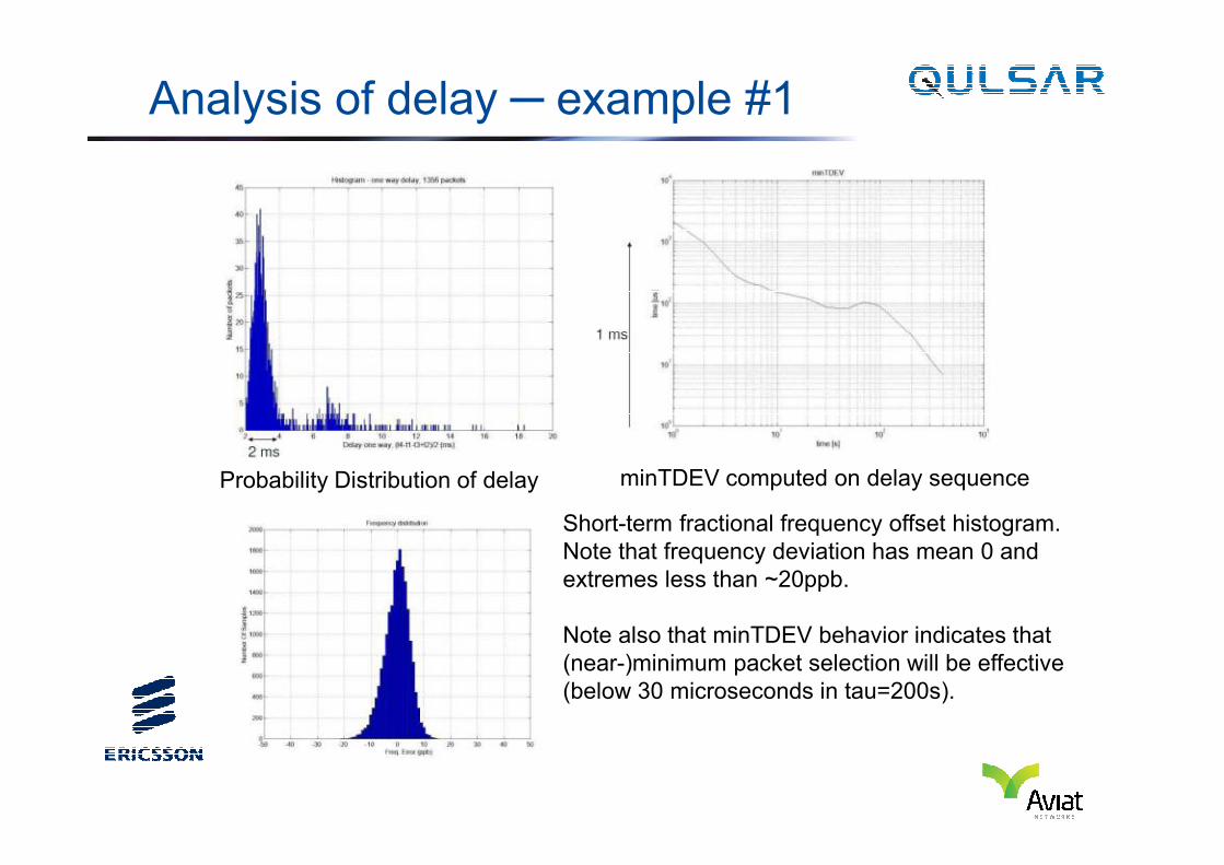
Analysis of delay ─ example #1
Probability Distribution of delay minTDEV computed on delay sequence
Short-term fractional frequency offset histogram.
Note that frequency deviation has mean 0 and
extremes less than ~20ppb.
Note also that minTDEV behavior indicates that
(near-)minimum packet selection will be effective
(below 30 microseconds in tau=200s).
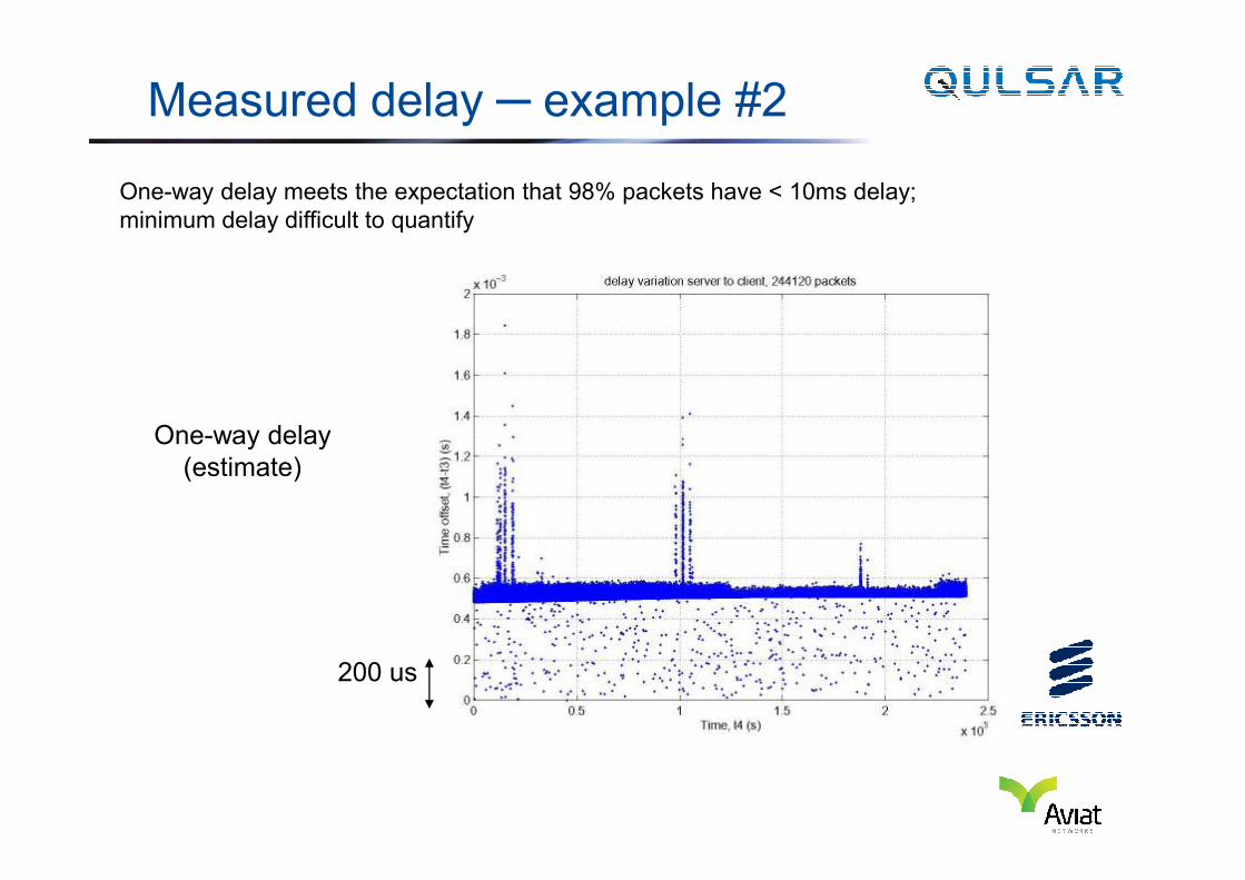
Measured delay ─ example #2
One-way delay
One-way delay meets the expectation that 98% packets have < 10ms delay;
minimum delay difficult to quantify
One-way delay
(estimate)
200 us
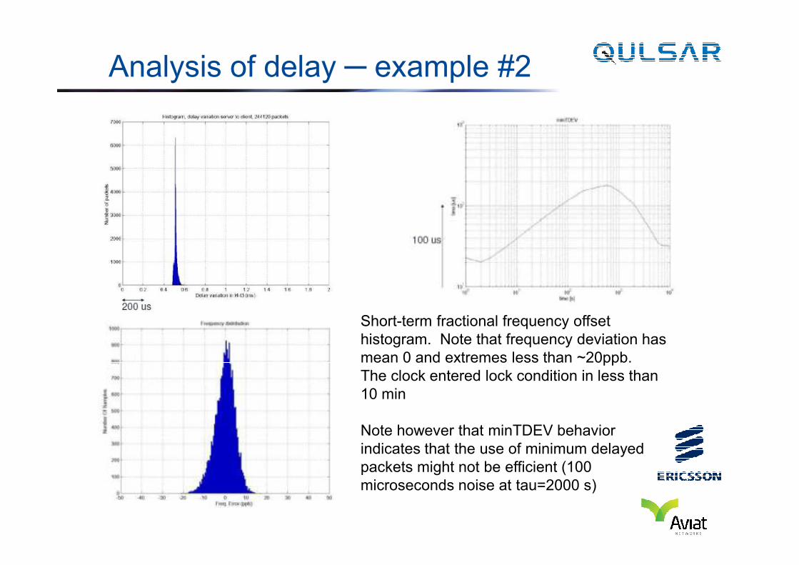
Analysis of delay ─ example #2
Short-term fractional frequency offset
histogram. Note that frequency deviation has
mean 0 and extremes less than ~20ppb.
The clock entered lock condition in less than
10 min
Note however that minTDEV behavior
indicates that the use of minimum delayed
packets might not be efficient (100
microseconds noise at tau=2000 s)