Embed Size (px)
Citation preview
Theoretical
Theoretical Computer Science 220 (1999) 67-91
Computer Science
www.elsevier.comflocate/tcs
Timing conditions for linearizability in uniform counting networks *
Nancy Lynch”, Nir Shavit a,b, Alex Shvartsman”.“~“, Dan Touitoubd
a MIT, Lu~orufar~ for Co~np. Science, 545 Technology Square, Cambridge, MA 02139, USA b Tel-Ark ~n~l~ersit~, School of mathematical Sciences, Department of ~orn~ater Science, Ramat Au&
Tel Aviv, 69978, Israel ’ Uniuersity of Connecticut, Computer Science and Engineering, 191 Auditorium Road, (1-155,
Storm, CT 06269, USA d nSOF, Israel
Abstract
Counting networks are concurrent data structures that serve as building blocks in the design of highly scalable concurrent data structures in a way that eliminates sequential bottlenecks and contention. Linearizable counting networks assure that the order of the values returned by the network reflects the real-time order in which they were requested. ~~~e~r~z~~~~~t~ is an important consistency condition for concurrent data structures, as it simplifies proofs and enhances compositional&y.
Though most counting networks are not linearizable, this paper presents a precise characteriza- tion of the timing conditions under which uniform non-linearizable networks exhibit linearizable
behavior. Uniformity is a common structuring property of almost all published counting net- works: a uniform network is made of “balancers” and “wires” so that each balancer lies on some path from inputs to outputs, and all paths from inputs to outputs have equal lengths. Our results include the following simple condition: if the time it takes a slow token to traverse a “wire” or “balancer” is no more than twice that of a fast token, the network is linearizable. Sur- prisingly, the timing measure in this condition is local to the individual ‘wires” and “balancers” of the network, that is, it is independent of network depth.
We use our timing measure to mathe~tically explain our empirical findings: that in a variety of highly concurrent execution scenarios tested on a simulated shared memory multiprocessor, the Bitonic counting networks of Aspnes, HerIihy, and Shavit exhibit completely linearizable behavior, and when linearizability is violated, the percentage of violations is relatively small.
Herlihy, Shavit, and Waarts have shown that counting networks that achieve linearizability under all circumstances must pay the penalty of linear time latency. Our results suggest that for systems in which timing anomalies occur infrequently, such linear delays may be an unnecessary
* Correspondence address: E-mail: [email protected]. ’ This work was supported by the following contracts and grants: ARPA N00014-92-J-4033 and F19628-
95-C-01 18, NSF 9225 1‘24~CCR, 9520298~CCR and 9804665~CCR, ONR-AFOSR F49620-94- I-01997, and AFOSR F49620-97-f-0337. A prclirni~~ version of this work appears as Co~nfj~~ networks are Pructicul~y
~~~ea~iza~~e in the Proceedings of the 15th Annual ACM S~~sium on Principles of Distributed Computing, Philadelphia, PA, May 1996, pp. 280-289.
0304-3975/99/S-see front matter @ 1999 Elsevier Science B.V. All rights reserved. PII: SO304-3975(98)00237-O

burden on applications that are willing to incur occasional non-~inea~zabil~~. @ 1999 EIsevier Science B.V. All rights reserved.
Keywords: Counting network; Timing analysis; Linearizability; Data structure; Empirical evaluation
1. Introduction
Counting networks [4] are a class of highly scalable structures used for concurrent
counting. Such networks allow the design of concurrent data structures in a way that
eliminates sequential bottlenecks and contention. Unlike queue-locks [21] and com-
bining trees [ 131 which are based on a single counter location handing out indices,
counting networks hand out indices from a collection of counter locations. To guaran-
tee that indices handed out by the separate counters are not erroneously “duplicated”
or “omitted,” one adds a special network coordination structure to be traversed by
processes before accessing the counters.
Counting networks [4] are constructed from simple computing elements called bal-
arzcers (see Fig. 1). Tokens arrive on the balancer’s input wires and are output on its
output wires. Intuitively one may think of a balancer as a toggle me~h~ism that, given
a stream of input tokens, repeatedly sends one token to the left output wire and one
to the right, effectively balancing the number of tokens that have been output. In order
to form a counting network, balancers are connected to one another by wires in an
acyclic fashion, in the same way comparators are connected to form a sorting network
[ 111. However, unlike in sorting networks, counting networks are asynchronous in na-
ture, that is, tokens arrive at the network’s input wires at arbitrary times, and traverse
the network with differing pace. Nevertheless, if the balancers are connected correctly,
a network having w consecutively numbered output wires will move input tokens to
output wires in increasing order mod&o W. Networks of balancers having this property
can easily be adapted to count the total number of tokens that pass through them.
Counting is done by adding a “local counter” to each output wire i, so that tokens
coming out of that wire are assigned numbers i, i + w, i + 2w, and so on.
On a shared memory multiprocessor, counting networks are implemented as data
structures in which balancers are represented as records and wires as pointers among
them. Tokens are “shepherded” by processors that traverse this pointer-based data struc-
ture from input pointers to output wires, finally incrementing the counter on the appro-
priate output wire. This implies that tokens may overtake one another on a wire and
that balancer and network traversal times are dependent on individual processor speeds
and variations in speeds.
A Bitonic counting network [4] has a layout isomo~hic to Batcher’s Bitonic sorting
network [7]. Bitonic costing networks for IZ processors have width w < n and depth
@(log* w) (all logarithms in this paper are to the base 2). Unlike combining trees,

N. Lynch et ul. I Theoretical Computer Science 220 (1999) 67-91 69
Fig. 1. A balancer and its input-output properties.
counting networks support complete independence among requests and are thus highly
fault tolerant. At peak performance their throughput is w, as w indices are returned
per time step by the independent counters. Unfortunately, counting networks suffer a
performance drop-off due to contention as concurrency increases, and the latency in
traversing them is a high @(log* w). There is a wide body of research on counting net-
works [24,9, 10, 12, 15, 17, 181. A recently developed form of counting network called
a Diffracting Tree [24] is based on a new type of distributed balancer implementation.
It has been shown to scale especially well, exhibiting low latency since its depth is
logarithmic in w.
Linearizability is a consistency condition for concurrent systems formulated by Her-
lihy and Wing [ 161. It requires that the values returned by access requests to a con-
current shared object reflect the order in which they were issued. The use of lin-
earizable data abstractions simplifies both the specification and the proofs of multiple
instruction/multiple data shared memory algorithms. As Herlihy and Wing explain, lin-
earizability generalizes and unifies a number of ad hoc correctness conditions in the
literature, and is related to (but not identical with) correctness criteria such as sequential
consistency [ 191 and strict serializability [22].
Herlihy et al. [ 151 defined the class of linearizable counting networks, networks that
assure that the order of the values returned by the network reflects the real-time order
in which they were requested. Linearizable counting lies at the heart of concurrent
timestamp generation, as well as concurrent implementations of shared counters, FIFO
buffers, priority queues and similar data structures. Unfortunately, for both the Bitonic
networks of Aspnes et al. [4] and the Diffracting Trees of Shavit and Zemach [24],
there exist worst case asynchronous schedules in which linearizability is violated. In
[15] linear depth linearizable counting network constructions were presented and shown
to be optimal, that is, any low contention counting network that is linearizable in all
executions must have linear depth.
I. 1. Timing and linearizability
This paper provides a characterization of the timing conditions under which low
depth non-linearizable counting networks become linearizable. It applies to semi-
synchronous and real-time systems [6] where upper and lower time bounds that limit
the extent to which one process can be slower or faster than others are known. As we
show, our characterization also extends beyond such systems and has implications in

70 N. Lynch et al. I Theoretical Computer Science 220 (1999) 67-91
the analysis of counting network linearizability in general asynchronous multiprocessor
systems. We believe that the linear time cost of designing counting networks achieving
linearizability under all circumstances may be an unnecessary burden on applications
that are willing to trade-off occasional non-linearizability for speed and parallelism.
In such systems an intelligent trade-off decision can be made with the help of clear
characterization of the parameters governing linearizability.
Our main result is a simple timing condition that is local to the individual wires and
balancers of the network. It quantifies the extent to which a network can suffer from
timing anomalies and still remain linearizable.
This result is interesting, since even a counting network of depth one exhibits non-
linearizable behavior. Consider the following scenario for a counting network consisting
of the balancer B and two atomic counters As and Ai with initial values 0 and 1, and
that count by 2: Token TO enters the balancer via ~0, exits via yc, and then is delayed.
Token Ti enters via xc and exits via yi and obtains the value 1 from the counter A,.
Token T2 enters via x0 and exits via yo and obtains the value 0 from the counter Ao. Finally, TO obtains the value 2 from Ao.
The behavior is not linearizable because the traversal of the network by T, completely
precedes T2, yet T2 returns a lower counter value.
We use a ci/cz timing model in the style of Attiya et al. [5]. Let ci be the minimum
time that it takes for a token to traverse a wire from balancer to balancer, let c2 be the
maximum such time, and assume that balancer transitions are instantaneous. This timing
model is general enough to capture standard message passing and shared memory
balancer implementations [4,24]. Alternately, one could attribute the Q/C, latency to
the balancer traversal and make wire traversal instantaneous. The two models can be
shown to be equivalent, and we choose to attribute delays exclusively to the wires as
this simplifies our modeling and presentation.
Our model is also similar to that of semi-synchronous systems (cf. Archimedean
distributed systems of Vitanyi [25]). One can view our setting as one in which each
token traverses a wire and a balancer on the local clock tick, where the local clocks
can tick not faster than every cl, and not slower than every c2 time units according to
some global clock.
A common structuring property of almost all published counting networks [24,9
12,15,18,17,23,24] is uniformity: each balancer of the network lies on some path
from inputs to outputs, and all paths from inputs to outputs have equal lengths.
We prove, in Section 3, the following properties for any uniform counting network
(explicitly constructible or not):
- If c2 ~2 . cl then the network is linearizable. This is so regardless of the network
depth.
- If c2 > 2 . cl then the network is linearizable if for any two tokens traversing the
network their traversals either overlap or they are separated by time t > h.(q -2.q), where h is the depth of the network.
- If a constant k > 2 is known a priori, such that c2 = k . cl, then given a counting
network of depth h we can extend this network by prefixing each of its inputs with
N. Lynch et al. I Theoretical Computer Science 220 (1999) 67-91 11
h(k - 2) l-input l-output balancers so that the resulting network is a linearizable
network of depth O(h).
In Section 4 we show that counting (Diffracting) trees and Bitonic counting networks
are not linearizable for c2 > 2.~1, and that one can create executions with large numbers
of non-linearizable operations.
Finally, in Section 5 we provide empirical measurements of the extent to which
timing can affect linearizability in Bitonic networks and Diffracting trees. These results
were collected on a simulated Alewife [l] shared-memory multiprocessor using the
Proteus [ 81 simulator.
We use our cl/c2 measure to mathematically support our experimental results: that
in a variety of “normal” situations, the Bitonic counting networks of Aspnes et al.
[4] exhibit linearizable behavior. In fact, for high concurrency levels, our results show
that even if one skews system timings by introducing large timing variations among
processes, the network rarely exhibits violations of linearizability. At low concurrency
levels we observed a significantly higher number of violations.
2. Models and definitions
We consider networks consisting of acyclically wired routing elements called bul-
ancers. We refer the reader to [4] for a more detailed presentation of the model and its
implications. For the sake of generality, our balancers are defined as multi-balancers
in the style of Aharonson and Attiya [2] and Felten et al. [ 121 (Fig. l), having e input
wires x0,x1,. . . ,x,-l and d output wires yo, ~1,. . . , yd_ 1. Slightly abusing notation, we
let xi (respectively yi) also serve as a state variable that stands for the number of
tokens that have entered (exited) via that wire.
A balancer passes tokens from input wire to output wire, maintaining a step property
on its output wires: in any state of the balancer, its output wires satisfy 0 < yi - yj < 1
for any i < j. This requirement is stronger than the standard one [4], since it implies
that token traversal through a balancer is atomic. However, we note that it is consistent
with the standard message passing and shared memory based balancer implementations
[4] and with Diffracting balancer implementations [24], as they all meet the specification
of a balancer with atomic transitions.
We further require that a balancer not create tokens spontaneously, that is, Cfzd xi 3
Cfi’ yi. A t t s a e in which CFz,i xi = Et=;’ yi is called a quiescent state.
To perform an increment operation on the network, a process routes a token from
input wire to output wire, traversing a sequence of balancers on the way. We define
a quiescent state of a balancing network with v input ports &Xl,. . . J-1 and w
output ports Yo, Yi, . . , Y,_, as a state in which all tokens that have ever entered it
have already exited. A counting network with w outputs is a network of balancers that
satisfies the following step property:
In any quiescent state, 0 <qYi - Yj <ql for any i < j.

N. Lynch et al. I Theoretical Computer Science 220 (1999) 67-91
The step property of counting networks is the cornerstone of the claims and proofs
we will present.
We now add timing to our model. The state transition of a balancer, i.e., the passing
of a token from the balancer’s input port to its output port, will be modeled as an
instantaneous event. While balancer transitions are instantaneous, transitions along a
wire connecting an output port of one balancer to an input port of another are not.
However, we assume that there is some cl > 0 that is the lower bound on time it
takes for a token to traverse a wire between two balancers. Similarly there exists a
c2 that is the upper bound on such time, where 0 < cl <CZ. Wires with the same
delay bounds are also used to connect the output wires of the network to a set of
counters added to it. Each output wire Yj of the network leads from a balancer whose
output wire is also a network output, to an atomic counter at its end. We identify this
counter with the output wire Yi. The input wires of a network are the input wires of
the balancers they connect to. Such balancers are called input balancers. We use the
term node to refer to a component of a network that may be either a balancer or a
counter.
We refer to w as the output width of the network. The tokens exiting from output
wire 5 are consecutively assigned the numbers i, i+w, i+2w, etc. The number assigned
to a token by a counter is called the token’s returned value.
Definition 2.1. A counting network is uniform if each balancer of the network lies
on some path from inputs to outputs, and all paths from inputs to outputs have equal
lengths.
We define the depth of a uniform counting network as the number of wires on the
path between any input balancer and output counter. The time t it takes for a token
to traverse a uniform network of depth h is bounded by: h . cl <t <h .c2. It is easy to
see, from the above definition, that for each balancer B, the lengths of all paths from
the input balancers to B are equal and the lengths of all paths from B to the output
balancers are equal, see Fig. 2. Note that there and in the remaining figures, we do
not show the counters attached to the outputs. For 1 <g < (h + 1) we also define the
g-th layer of a network to be the collection of nodes (balancers or counters) whose
distance from the inputs is g - 1.
In the proofs, without loss of generality, we sequentially number the tokens traversing
the network according to the time of their entry (ties are broken arbitrarily).
An execution or execution sequence of a network is a sequence E = el, e2,. . . of
instantaneous transition events ei = (T, B) corresponding to a token T traversing a
balancer or counter B. We associate history variables with tokens and balancers to
capture their implicit knowledge about the execution. The history variables are sets
of token ids. A history variable HT is associated with each token T, and HB with
each balancer B. For every execution E the values of these variables are computed
inductively as follows, where Hi and Hk denote the values of Hs and HT after the
event ei:

N. Lynch et al. I Theoretical Computer Science 220 (1999) 67-91 73
Fig. 2. Equal length paths lead to any balancer in a uniform network
_ At the beginning of the execution, we define Hj = 0 and HF = {T}. In other words,
at the beginning of the execution the knowledge of every balancer is an empty set
and the knowledge of every token consists of the token’s own identifier. _ The inductive step is as follows: If ei = (Z’,B), then HL = Hk = Hk-’ U HL-' .
Intuitively, the token T and the balancer B combine their knowledge as the result
of e,.
For every other token T’ # T and balancer B’ # B, we define Hi, = Hk7’ and
H;, = H;;‘.
Definition 2.2. A timing schedule S for an execution of a uniform network of depth h and input width v is a triple (K, L, Q). K is the set of token ids produced by sequentially
numbering the tokens starting with 1 and based on their arrival times. L : K + {XI : 0 d i < IJ} is a function such that for a token T, L(T) is the input balancer on which
the token enters the network. Q : K x [ l..(h + l)] + R (where R is the reals) is the
function such that Q(T, g) is the real time instant when the token T passes through a
node in layer g of the network.
Adapting the definition of Herlihy and Wing [ 161 to counting networks:
Definition 2.3. An execution of a counting network is linearizable if for any two tokens
that traverse the network one completely after another (non-overlapping in time), the
earlier token obtains a smaller value than the later one.
Definition 2.4. A counting network is linearizable if every execution of the network
is linearizable.
We now introduce the notion of non-linearizable operations. Consider an execution in
which the network traversal operation a completely precedes another traversal operation
j?, but a returns a higher value than /3. Clearly such an execution is not linearizable. In
the definition below we ascribe the non-linearizablilty of the execution to the operation
B:
Definition 2.5. Given an execution of a counting network, we say that a traversal
operation /3 and its associated token are non-linearizable, if there exists some other

14 N. Lynch et al. I Theoretical Computer Science 220 (1999) 67-91
traversal operation a completely preceding fi in time, whose associated token has a
higher returned value than /J.
We choose to define j3 as the non-linearizable operation and not CI since this al-
lows us to determine whether or not an operation is non-linearizable as soon as it
completes. Furthermore, if instead tx were defined to be the non-linearizable traver-
sal operation, this would lead to non-intuitive situations where a single operation can
cause all preceding operations to become non-linearizable if it returns a sufficiently
low value.
It is easy to see that for any execution sequence, if we remove all non-linearizable
traversal operations the remaining sequence of operations will contain no violations of
linearizability. 2 However, such sequence of operations might not correspond to a valid
execution of a counting network, since it could contain gaps.
The following definition quantifies non-linearizability of finite executions:
Definition 2.6. The fraction of non-linearizable operations in a finite execution is de-
fined to be the number of non-linearizable operations divided by the number of com-
pleted operations in the execution.
It follows from the definitions above that this fraction is an upper bound on the
fraction of operations whose removal yields a linearizable execution trace.
3. A characterization of linearizability for counting networks
In this section and the next, we show that the ratio Q/C, plays a key role in deter-
mining whether a uniform counting network is linearizable.
We begin by proving several lemmas that will be used to derive our main result,
that uniform networks are linearizable for c2 <2cl. The first lemma shows that in
any counting network, when a token completed traversing the network, it has implicit
knowledge about the “existence” of a certain minimum number of other tokens.
Lemma 3.1. Let N be a counting network with w output ports Y,,. . . , Y,_I. If the token T is the ath token to exit on 6, then IHT( > w(a - 1) + i + 1 following its transition onto I$
Proof. The proof is by contradiction, We start by defining the notion of events injlu- encing other events. For a pair of events e and e’ in an execution E, we say that e
*In general it may be possible to remove fewer operations (whether linearizable or not) to eliminate
all instances of non-linearizability. For example, consider an execution consisting of three time-disjoint
operations CC, fi and ‘/ that return the values 3, 1 and 2, in that order. According to our definition, B and 7 are non-linearizable. Removing both of them yields a sequence consisting of a alone, thus removing all
instances of non-linearizability. However, if we remove x instead, then p and y become linearizable.
IV. Lynch et al. I Theoretical Computer Science 220 (1999) 67-91 75
in$uences e’ if there is sequence of events S = et, e2,. . . , e, such that (1) S is a subse-
quenceofE,(2)e=et ande,=e’and(3)foreveryk=l,...,n-1 ifek=(Tk,Bk)
and ek+l = (Tk+t,&+t), then either Tk = Tk+r Or & = &+,.
We now assume that there exists an execution E, in which T is the ath token to
exit on Yj, but IHrI < w(a - 1) + i + 1. We fix E and construct a new execution
E’ in the following way: Let E’ be the projection of E consisting consisting of all
events involving T, and all the events that influence these events. From the definition
of implicit knowledge, it is clear that E’ contains events involving only the tokens
found in HT during the execution.
We claim that E’ is a possible execution of the counting network in which the
participating tokens and nodes cannot distinguish between E’ and E. We show this by induction on all the prefixes of E’. The base case for the empty
prefix is trivial. For the inductive step we assume that the length of E’ is positive and
that the prefix of E’ of length n - 1, for n > 1, is a possible execution of the network.
We now consider the prefix e{,ei . . . , eh of E’, where eh = (S, D). Now consider the sequence er , e2,. . . , e, such that it is the prefix of E that ends
with e, = e:. By the definition of E’, we know that all the events involving either
S or D in et,ez,... e,_ 1 are contained in e{, ei, . . . , eA_, . By the induction hypothesis,
ei,ei,...,eL_, is a possible execution of the counting network in which the participating
tokens and nodes cannot distinguish between this prefix and the prefix et, e2,. . . e, of
E, where the event ei is eL_, .
Note that by the definition of E’ the subsequence ei+r , . . . , e,_ 1 of E, does not include
any events involving S or D. Therefore, neither S nor D can distinguish between I the execution el,, ei, . . . , e,_, and the execution et, e2,. . . , e,_ I. Because (S, D) is next
event after e,_l in E, the sequence e{, ei, . , eA_,, (S,D) is a possible execution of
the counting network.
In E’, T is still the ath token to exit on K. Since only the tokens of HT participate in
E’, any completion of E’ in which no new token enters the network leads to a quiescent
state with the step property violated. This is so because if a tokens exit on Yi, then it
is impossible to establish the needed step property with fewer than w(a - 1) + i + 1
tokens. 0
The next lemma shows that the implicit knowledge in the history variables can only
reflect information propagation at the maximum pace of 1 wire per cl time units.
Lemma 3.2. Let N be a uniform counting network of depth h. For any execution E = el, e2,. . ., if ek = (T, B) occurs at time t, where B is a node in layer (g + 1 ), for 0 by d h then Hj contains only tokens that enter the network by time t - g ’ cl.
Proof. By induction on g. The base case for g = 0 is trivial. Assume the lemma holds
for g - 1. We now show it holds for g.
Assume there is an execution sequence E = el, e2,. . . , ek, . . ., containing a transition
event ek = (T, B) that occurs at time t. Assume also that [{ej : 1 Q’ < k A ej =
16 N. Lynch et al. I Theoretical Computer Science 220 (1999) 67-91
(T,B,))I = Y, h’ h w tc means that token T traverses g balancers and wires en route to
B. From the definition of historical knowledge, H; = H;-’ U If;-‘.
Consider the tokens in HF-‘. This set reflects T’s knowledge after traversing g - 1
wires. By the induction hypothesis and because it takes at least ci time to traverse a
wire, all tokens in H:-’ enter the network by time (t - cl) - (g - 1)q = t - g . cl. Now consider the tokens in Hj-' . This set consists of the accumulated knowledge
of the tokens that traversed B. Because the network is uniform, each token in Hi-’
traverses g wires before reaching B. Since each such token reaches B by time t, it
reaches the previous balancer (there is such a balancer because g > 0) by time t - cl
and by the induction hypothesis it enters the network by time (t - cl) - (g - 1)q =
t-g.ci. q
The next result combines the lemmas above:
Lemma 3.3. Let N be a untform counting network of depth h with w outputs. If at time t, token T exits on output x., and it is the ath token to exit through this output
wire, then at least w(a - 1) + i + 1 tokens enter the network by time t - h. cl.
Proof. Let ej = (T, yi) (recall that we identify the counter at output K with x).
Lemma 3.1 establishes iHi/ 3w(a - 1) + i + 1. Lemma 3.2 establishes that the tokens
in Hi = H& enter the network by time t - h . cl. 0
In the next lemma we show that if the tokens in a set K1 enter a network N by
time t and proceed according to time schedule Qi, and the tokens in the set K2 enter
after t, then any tokens that enter after t can only increase the number of tokens that
exit on any output of any balancer B as the result of Qi.
Lemma 3.4. Let t be a time instant, and S1 = (Kl,L,,Ql) and S, = (K1 UKz,&,Qz)
be two timing schedules for a uniform counting network N, such that K1 n K2 = 0, b Lb, Ql C Q2 and QdTl, l)Gt < QdT2,l)f or all tokens T, E K1, T2 E K2. If B is a balancer within layer g + 1 of N, where 0 6 g <h, then by time t + g. c2 the number of tokens that traverse any of B’s outputs in SZ is no smaller than the number of
tokens that traverse the same output of B in S,.
Proof. By induction on g. For g = 0 the lemma follows trivially from the fact that
in Si and Sz, by time t only the tokens in K1 enter and they enter through the same
input balancers.
Assuming the lemma holds for g, we show it holds for g + 1. Consider a node B within the layer g + 2. Since N is uniform, all of B’s inputs are connected to the
outputs of some balancers within the layer g + 1. By the induction hypothesis, by time
t + gc2 the number of tokens that exit on any of these outputs in S2 is no smaller
than the number that exit on the same outputs in Si. Since it takes at most c2 time
to traverse a wire from one layer to the next, by time t + (g + l)c2 the number of
N. Lynch et al. I Theoretical ~orn~~t~r Science 220 (1999) 67-91 i-l
tokens that enter any of the inputs of B in S2 is no smaller than the number of tokens entering the same inputs in St.
In any execution, the number of tokens exiting any of the outputs of a balancer is deterministically established from the sum of the number of tokens that enter the inputs of the balancer. Since Qt C Qz, for any balancer, between time t + gc2 and t + (9 + 1 )c2 there are at least as many tokens transitioning from its inputs to each of its outputs in S, as in SI. 0
For the next two proofs, given a counting network of width w, we define #’ to be the number of tokens that exit on each of the network outputs K (0 di < w) once m tokens enter and exit the network. We use the property of counting networks that q:t
is uniquely defined by the formulas Ezi’ qr = m and 0 dql - qy G 1 for i < j [4J.
Lemma 3.5. Let N be a uniform counting network of depth h and width w. lj” m tokens enter N by time t, then bJ> time t f h . c2 the number of tokens that exit on
each output Yi is at least qy.
Proof. Let St = (Kt,Lr, Q) be a timing schedule with IKt ( = m and Qr(7’, 1) <t for T f Ki. It takes at most h . c2 time for a token to traverse the network. Therefore, any of the m tokens that enter the network by time t must exit the network by time t’ = t + h . c2. Since by the definition of 5‘1 no other tokens entered the network, it is in a quiescent state and the number of tokens exiting on each output Yt is exactly qr.
Suppose additional tokens enter the network after time t. Let S, be the timing sched- ule that describes an execution with additional tokens entering after time t. By Lemma 3.4 with g = h, for each output 5, the new number of tokens that exit in S2 is no smaller than the number that exit in St, and is therefore at least 47. II
The following is our main theorem on the linearizability of uniform counting net-
works.
Theorem 3.6. If tokens T, and Tz trauerse a untorn counting network of depth
h during periods [to, tl] and [tz, ts], respectively, in an execution in w~jch tl + h .
(~2 - 2~1) < t2, then TZ has a higher returned value than T,.
Proof. Suppose ai is the number of tokens that exit by time tl on output Yi for 0 <i < w. We define r as follows:
r=max{i:Obi < wAai=maX{aj:O<j < w}},
i.e., r is the largest output index such that a, is the largest number of tokens that exit on any output.
By Lemma 3.3, there are at least m = w(a, - 1 )+r + 1 tokens that enter the network no later than time t = tl - h f et (see Fig. 3), and Zi is among these tokens. Let K be the set of these tokens.
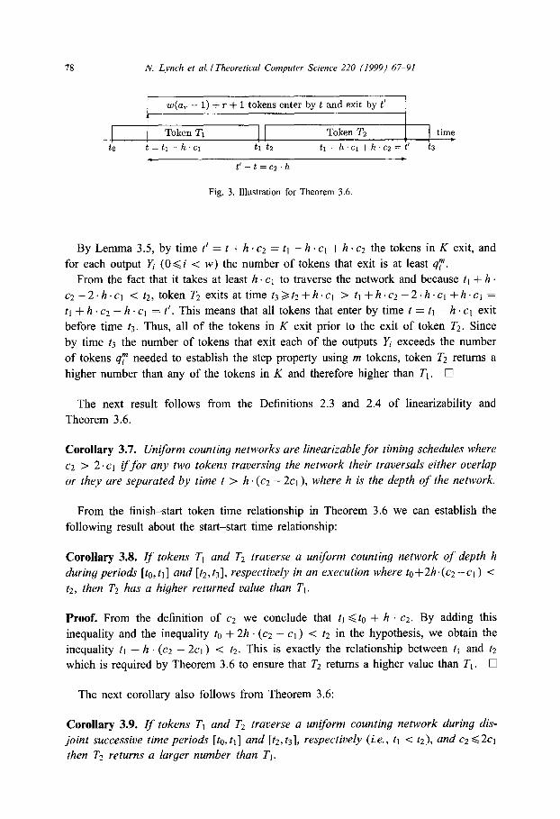
78 N. Lynch et al. I Theoretical Computer Science 220 (1999) 67-91
w(a, - 1) + T + 1 tokens enter by t and exit by t’ ,
to
Token Tl Token TZ time c
t=tl-h.cl t1 tz t1 - h Cl + h . c2 = t’ t3
. c
t’ - t = c2 h
Fig. 3. Illustration for Theorem 3.6.
By Lemma 3.5, by time t’ = t + h . c2 = tl - h . cl + h .c2 the tokens in K exit, and
for each output K (O<i < w) the number of tokens that exit is at least 47. From the fact that it takes at least h. cl to traverse the network and because tl + h .
c2-2.h.cl < t2, token T2 exits at time t3>t2+h.cl > tl+h.c2--2.h.c1 +h.cl = tl + h . c2 - h . cl = t’. This means that all tokens that enter by time t = tl - h . cl exit
before time t3. Thus, all of the tokens in K exit prior to the exit of token T2. Since
by time t3 the number of tokens that exit each of the outputs K exceeds the number
of tokens qT needed to establish the step property using m tokens, token T2 returns a
higher number than any of the tokens in K and therefore higher than Tl. 0
The next result follows from the Definitions 2.3 and 2.4 of linearizability and
Theorem 3.6.
Corollary 3.7. Uniform counting networks are linearizable for timing schedules where c2 > 2.~1 iffor any two tokens traversing the network their traversals either overlap or they are separated by time t > h. (Q - 2cl), where h is the depth of the network.
From the finish-start token time relationship in Theorem 3.6 we can establish the
following result about the start-start time relationship:
Corollary 3.8. Zf tokens Tl and T2 traverse a unform counting network of depth h during periods [to, tl] and [tz, t3], respectively in an execution where to+2h.(cz -cl ) < t2, then T2 has a higher returned value than Tl.
Proof. From the definition of c2 we conclude that tl <to + h ~2. By adding this
inequality and the inequality to + 2h . (~2 - cl) < t2 in the hypothesis, we obtain the
inequality tl + h . (~2 - 2~1) < t2. This is exactly the relationship between tl and t;!
which is required by Theorem 3.6 to ensure that T2 returns a higher value than Tl. 0
The next corollary also follows from Theorem 3.6:
Corollary 3.9. Zf tokens Tl and T2 traverse a uniform counting network during dis- joint successive time periods [to, tl] and [t2, t3], respectively (i.e., tl < t2), and c2 ~2~1 then T2 returns a larger number than Tl.
N. Lynch et al. I Theoretical Computer Science 220 (1999) 67-91 79
Proof. If c2 <2ci, then h.(c~--2~1) GO. By adding this inequality and the the inequality
tl < t2 we again obtain the relationship between tl and t2 that allows us to use Theorem
3.6 to ensure that T2 returns a higher value than TI. 0
Together with the definition of linearizability, this leads to our main local lineariz-
ability criteria for uniform networks:
Corollary 3.10. Uniform counting networks are linearizable for any timing schedule where c2 ~2. cl.
This implies that Bitonic counting networks [4], Periodic counting networks [4], the
networks of [9, 181 are all linearizable for c2 g2 . cl. It also implies that counting
and Diffracting trees [24] and the uniform trees of Busch and Mavronicolas [lo] are
linearizable for c2 < 2 . cl.
We now consider a modification allowing to turn any uniform depth counting net-
work into a linearizable network given that c2 <k . cl for some k >, 2.
Corollary 3.11. Given a uniform counting network of depth h, another uniform count- ing network of depth [h. (k - 1 )1 can be constructed so that it is linearizable for any ka2 such that c2<k’c1.
Proof. Given the original network, we attach in front of each of its inputs a path of
length [h . (k - 2)] of l-input l-output “balancers” wired one after the other. The
tokens traversing such balancers simply proceed from one to the next. For any two
tokens that traverse the new network in a time-disjoint fashion, their traversals of the
original (sub)network are such that the second token enters it at least [h(k - 2)lcl 3 h(cz/q - 2)q = h . c2 - 2h . cl time after the first token exits. By Theorem 3.6, the
second token returns a higher value.0
4. Limits on linearizability of trees and bitonic counters
We now show some limitations on the linearizability of Diffracting trees [24] and
Bitonic counting networks [4] by constructing execution scenarios under which they
exhibit non-linearizable behavior.
Theorem 4.1. Counting and Diffracting trees are not linearizable if c2 > 2. cl.
Proof. Let h be the depth of the tree and let E > 0 be such that c2 = (2 + E) . cl. We
consider an execution in which the first two tokens, TO and T,, enter the tree at the
same time to (we visualize the tree on its side with its root to the left and the leaves on
the right). Without loss of generality, let TO go up (corresponding to the root balancer
transition from 0 to 1) and Tl go down (the balancer transition from 1 back to 0), i.e.,
TO precedes Tl. After traversing the root, TO proceeds at the slowest possible pace of

80 N. Lynch et al. I Theoretical Computer Science 220 (1999) 67-91
one wire per c2 time, while ri proceeds at the fastest possible pace of one wire per
ci time. Ti reaches the topmost leaf of the bottom subtree at time ti = to + h . cl and
returns the value 1 (by the definition of the counting tree and cl).
Immediately after 2’1’s exit, a wave of 2h - 1 tokens enters the tree, say at time
t:! = tl + 6 > tl. We choose 6 to be such that 0 < 6 < E. These tokens proceed at
the fastest possible pace of 1 wire per ct time. Of these tokens, 2h-1 tokens go to the
upper subtree and the remaining 2h-’ - I tokens go to the lower subtree.
Since the token TO is slow, it reaches a leaf at time t4 = to + h + ~2. The second
wave of fast tokens reaches the leaves at time t3 = t2 + h 1 cl = t1 + 6 + h . cl =
to+2h.cl+6=to+h.(c;!-cl&)+6=to+h.c2--clhr:+6. Sincewechose6such
that 0 < 6 < E, the inequality can be further simplified to t3 < to + h 3 c2 = t4. Thus
t3 < 4 and these fast tokens reach the leaves ahead of TO. Since we have 2h-1 tokens
in addition to Z’a traversing the top subtree, at least one token reaches the topmost leaf
of the tree and returns the value 0. This token traverses the counting tree completely
after TI exits, but returns a smaller value. 0
We now consider Bitonic networks.
Lemma 4.2. Let TO be theJirst token to enter a Bitonic taunting network. Suppose TO
enters through input X0 and completely traverses the network alone. Zf subsequently tokens T1 and T2 enter the network in this order through X0, then: (a) the balancer that is attached to X0 is the only balancer that both TI and T2 pass through, (b) TO exits through output wire Yo, T, through output wire Y, and TI through output wire
Y2 (mod w).
Proof. By induction on the width w of the network: The base case is trivial for w = 2
with a single balancer and two counters (we only need to note that outputs ya and y2
are the same for this network).
Assuming the lemma holds for some width w > 2, we prove that it holds for networks
of width 2w. The inductive step is depicted in Fig. 4, and the balancer and exit
labels below refer to that figure. We use the inductive construction of Bitonic counting
networks as in [4]. Bitonic[2w] is made of two Bitonic[w] networks, two Merger[w]
1 Bitonic[2w]
Fig. 4. Inductive step for Lemma 4.2.

N. Lynch et al. I Theoretical Computer Science 220 (1999) 67-91 81
merging networks and an additional w balancers. Even-numbered outputs of Bitonici [w] are connected to the first w/2 inputs of Mergerr[w] and odd-numbered outputs of Bitonicz[w] are connected to the last w/2 inputs of Merger1 [w]. The rest of the outputs are similarly connected to Mergerz[w]. The outputs of the two mergers are then shz.@ed into a row of w balancers whose outputs are the outputs of Bitonic[2w].
By the inductive hypothesis for Bitonicr[w], token To exits via output tli,o, Ti via ur,t and T2 via ur,~ {note that for w = 2 the output ~li,o is the same as 2~). By the cons~ctio~ of Bitonic[2w], To and TZ enter Merger1 [w] via its first balancer. Since these are the only two tokens to enter Mergerr[w] and since they traverse the merger one after the other, TO must exit via vi,0 and T, via ui,i, else Bitonic[2w] will not reach a quiescent state in the execution where TO is the only token. Similarly, T1 exits via v2,a of Mergerzrw]. In the final row of balancers, TO and T, traverse Bt, and T2 traverses 82 _
To show (a) we observe that Ti and Tz may only traverse the same balancer inside Bitonicr[w], and by the inductive hypothesis, Bo is the only such balancer.
To show (b), we observe that TO traverses the network alone and it reaches Bi first and exits via Yo, and so TI necessarily exits via Yr. The only remaining token T2 exits via Yz. 0
Theorem 4.3. Bitonic counting networks are not linearizahle if 13 > 2 . cl,
Proof. In the example in Section 1 we established that a network of width 2 consisting of a single balancer and two counters is not linearizable, and it is easy to see that this is so for any CI and cz such that c2 > 2.~1. Below we consider networks with w > 2. We choose E, 6i,S2 > 0 such that 6, + 62 < E, and we let c2 = 2 . CI + c.
Using the framework of Lemma 4.2, we deploy the three tokens TO, Tl, and T2 according to the following scenario. Starting in the initial state, we let TO enter via the input X0 and completely traverse the network and exit via the output Ye thus returning the value 0. Following this, at some time tl, token Ti also enters via X0, and T2 enters via X0 immediately behind Ti at time cl+61 for some 61 > 0. We let Ti proceed at the slowest possible pace of 1 wire per c2 time, while T2 proceeds at the fastest possible pace of 1 wire per cl time. This means that T, exits at time ti = tl + 2h s cl + hc, and T2 exits at time t; = tl -I- 6, + h . cl.
By Lemma 4.2, the paths that Tl and Tz traverse have no balancers in common, with the exception of the first balancer in their paths. Thus, in the execution fragment that follows and does not include these tokens’ traversal of the first balancer, T, is not injhenced by T2 and still proceeds to the exit Y1.
As soon as T2 exits via YZ and obtains the counter value 2, w fast tokens enter the network at time t3 = ti + 62 for some ~52 > 0. Regardless of these tokens’ paths, they exit the network at time t$ = t3 + h . cl. Since 61 + by < E, these tokens exit before the slow token T2.
During this execution, the network is traversed by w + 3 tokens. If no other tokens enter the network, then each of outputs Yo, Yi, and Y;, has each two tokens that exit

82 N. Lynch et al. I Theoretic& Computer Science 220 (1999) 67-91
Fig. 5. Inductive construction of Bitonic[w] for Theorem 4.4 (wires are omitted).
through it, and outputs Y,, . . . , Y,_ 1 each have one. Thus one of the fast tokens exits
via Yt and because it is faster than T1, it obtains the counter value 1, while TI obtains
the value 1 + w. As a result the fast token obtains a lower value than T2. 0
As we will see in the experimental results Section 5, when the ratio cz/cr increases
beyond 2, the percentage of non-linearizable operations also increases. Below we show
that for Bitonic networks there can be a large fraction of tokens that exhibit non-
linearizable behavior for certain ratios of q/c,:
Theorem 4.4. Bitonic counting networks are not linearizable if c2 > i(3 + log w) ’ cl,
where w is the width of the network. Moreover, for such c2 and cl there exists an execution scenario with 3w/2 tokens such that w/2 tokens result in non-linearizable
operations.
Proof. The Bitonic counting network [4] of width w, Bitonic[w], has depth h =
i[log w . (log w + l)]. The network consists of two stages (see Fig. 5). The first stage
includes two Bitonic[w/2] networks of depth h, = h - log w connected in parallel to
the second stage that is the merging network of depth h2 = log w, Merger[w].
Merger[w] consists of a row of balancers connected to two Merger[w/2] mergers
(for details see [ll]). Note that this inductive construction of the merger is different
from, but isomorphic to the construction in Fig. 4. The construction we use here yields
a clearer proof.
A non-linearizable schedule is constructed as follows: The first wave of w/2 tokens
enters Bitonict[w/2] network at the same time and proceeds in lock step at some pace
to the exits of the first stage. The second wave of w/2 tokens enters the same network
immediately behind the first wave after a small delay 6 > 0.
As soon as the first wave enters Merger[w], it slows down to the slowest possible
pace of one wire per c2 time. This wave proceeds to the Mergert[w/2] sub-component
of the merger after passing through the first row of balancers of Merger[w].
Similarly, the second wave of w/2 tokens proceeds to Mergerz[w/2], except that it
proceeds at the fastest possible pace of one wire per cl time. As soon as the second
wave exits, a third wave enters Bitonic[w] as the first two waves.
The third wave of w/2 tokens proceeds in lock step at the fastest pace of one wire
per cl time to the exits. Therefore this wave exits through the first w/2 exits.
N. Lynch et (11. I Theoretical Computer Science 220 (1999) 67-91 83
It takes the first wave tl > h2 . c2 = c2 . logw time to reach the exits. It takes the
second wave t2 = h2 . cl = cl . log w time to exit. It takes the third wave t3 = h . cl =
cl .~[logw.(logw+ l)] time to traverse the entire network. Since c2 > 3(3+logw).ct,
we have that tl > t2 + t3. Thus the third wave passes the first wave on the final wire out
and returns counter values that are all lower than those obtained by the second wave.
There are three waves of w/2 tokens out of which w/2 tokens are non-linearizable. 0
We have shown specific scenarios in which the violations of local timing conditions
lead to non-linearizable executions in important classes of uniform counting networks.
The work of Mavronicolas et al. [20] shows how violations of timing conditions lead
to non-linearizability in general counting networks (see Section 6).
5. Empirical evaluation of linearizability
We evaluated the linearizability of counting networks on a simulated distributed-
shared-memory machine similar to the MIT Alewife of Agarwal et al. [l]. Alewife is a
large-scale multiprocessor that supports cache-coherent distributed shared memory and
user-level message-passing. The nodes communicate via messages on a two-dimensional
mesh network. A Communication and Memory Management Unit on each node holds
the cache tags and implements the memory coherence protocol by synthesizing mes-
sages to other nodes. Our experiments make use of the shared memory interface only.
To simulate the Alewife we used Proteus, 3 a multiprocessor simulator developed
by Brewer et al. [8]. Proteus simulates parallel code by multiplexing several parallel
threads on a single CPU. Each thread runs on its own virtual CPU with accompanying
local memory, cache and communications hardware, keeping track of how much time
is spent using each component. In order to facilitate fast simulations, Proteus does not
do complete hardware simulations. Instead, operations which are local (do not interact
with the parallel environment) are run uninterrupted on the simulating machine’s CPU
and memory. The amount of time used for local calculations is added to the time spent
performing (simulated) globally visible operations to derive each thread’s notion of the
current time. Proteus makes sure a thread can only see global events within the scope
of its local time.
5.1. Implementation and experimentation methodology
For our benchmarks, we implemented the Diffracting tree [24] and the Bitonic count-
ing network [4] in shared memory. Both types of data structures gave each simulated
processor with one of the two possible timing characteristics. The first kind allowed
the processors to traverse the network unimpeded. The second kind introduced a time
delay following the traversal of a balancer. This delay models the network delays or
3 Version 3.00, dated February 18, 1993.
84 N. Lynch et ul. I Theoretical Computer Science 220 (1999) 67-91
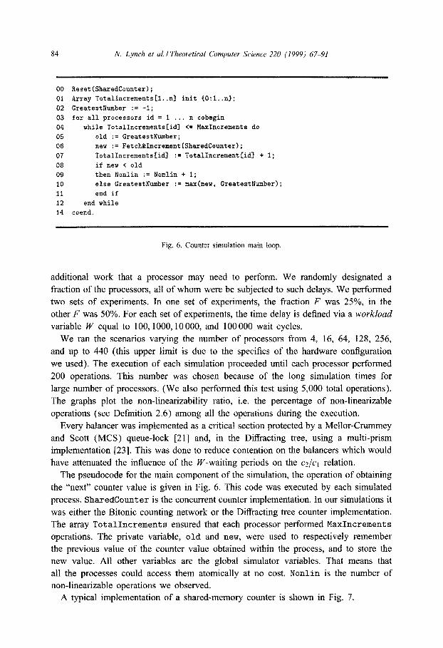
00 Rsset(SharedCounter); 01 Array TotalKncrements[l..n] init {O:l..n); 02 GreatestNumber := -1; 03 for all processors id = 1 . . . n cobegin
04 while TotalIncrements[idl <= MaxIncrements do 05 old := GreatestNumber;
06 new := Fetch&Increment(SharedCounter);
07 TotalIncrements [id] := TotalIncrement [id] + 1;
08 if new < old
09 then Nonlin := Nonlin + 1;
IO else GreatestNumber := max(new, GreatestNumber)
11 end if
12 end while 14 coend.
Fig. 6. Counter simulation main loop.
additional work that a processor may need to perform. We randomly designated a
fraction of the processors, all of whom were be subjected to such delays. We perfo~ed
two sets of experiments. In one set of experiments, the fraction F was 25%, in the
other F was 50%. For each set of experiments, the time delay is defined via a workload
variable W equal to 100, 1000,lO 000, and 100 000 wait cycles.
We ran the scenarios varying the number of processors from 4, 16, 64, 128, 256,
and up to 440 (this upper limit is due to the specifics of the hardware configumtion
we used). The execution of each simulation proceeded until each processor performed
200 operations. This number was chosen because of the long simulation times for
large number of processors. (We also performed this test using 5,000 total operations).
The graphs plot the non-linearizability ratio, i.e. the percentage of non-linearizable
operations (see Definition 2.6) among all the operations during the execution.
Every balancer was implemented as a critical section protected by a MeIlor-C~mey
and Scott (MCS) queue-lock [Zl] and, in the Diffracting tree, using a multi-prism
implementation [23]. This was done to reduce contention on the balancers which would
have attenuated the influence of the W-waiting periods on the CZ/CI relation.
The pseudocode for the main component of the simulation, the operation of obtaining
the “next” counter value is given in Fig. 6. This code was executed by each simulated
process. SharedCount er is the concurrent counter implementation. In our simulations it
was either the Bitonic counting network or the Diffracting tree counter implementation.
The array TotalIncrements ensured that each processor performed MaxIncrements
operations. The private variable, old and new, were used to respectively remember
the previous value of the counter value obtained within the process, and to store the
new value. All other variables are the global simulator variables. That means that
all the processes could access them atomically at no cost. Nonlin is the number of
non-linearizable operations we observed.
A typical implementation of a shared-memory counter is shown in Fig. 7.

N. Lynch et al. /Theoretical Computer Science 220 (1999) 67-91 85
type balancer is
begin
state: regular or Diffracting balancer state
next: array [O..d-11 of ptr to balancer
end
constants
width: global integer
input : global ptr to some input wire of a Bitonic network or binary tree of balancers
1 function fetchkincro: integer 2 begin
3 b:= input
4 while not leaf(b)
5 b := traverse-balancer(b) 6 endwhile
7 i := increment_counter_at_leaf(b)
6 return i * width + number_of_leaf(b)
9 end
Fig. 7. A Shared-Memory tree-based counter implementation
We present the empirical data by charting the non-linearizability ratio as the function
of the number of processors. In each of our experiments, we compute the average time
it takes for a processor to traverse a balancer and a wire when the workload W = 0. We
use this average as the approximation of cl in the presentation. Note that using such
average is conservative - e.g., using the minimum value for such traversal would cause
an increase in ~/et ratio and thus “excuse” or “explain” more of the non-linearizable
operations observed in some scenarios. Using this definition of cl, we compute c2 as
(Average-cl + Workload)/Average-cl = 1 + Workload/Average-q. The absolute values of the average cl vary between the Bitonic network and the
Diffracting tree due to the difference in the processing time associated with the prism
in the Diffracting tree implementation. For ease of presentation, all data is normalized
with respect to the average cl in the execution. To illustrate the ratio Q/C, (et divided
by 13) we present the normalized c2 and also the normalized standard deviation for cl
in the form Standard-deviationlAverage-cl .
5.2. Presentation and assessment of empirical data
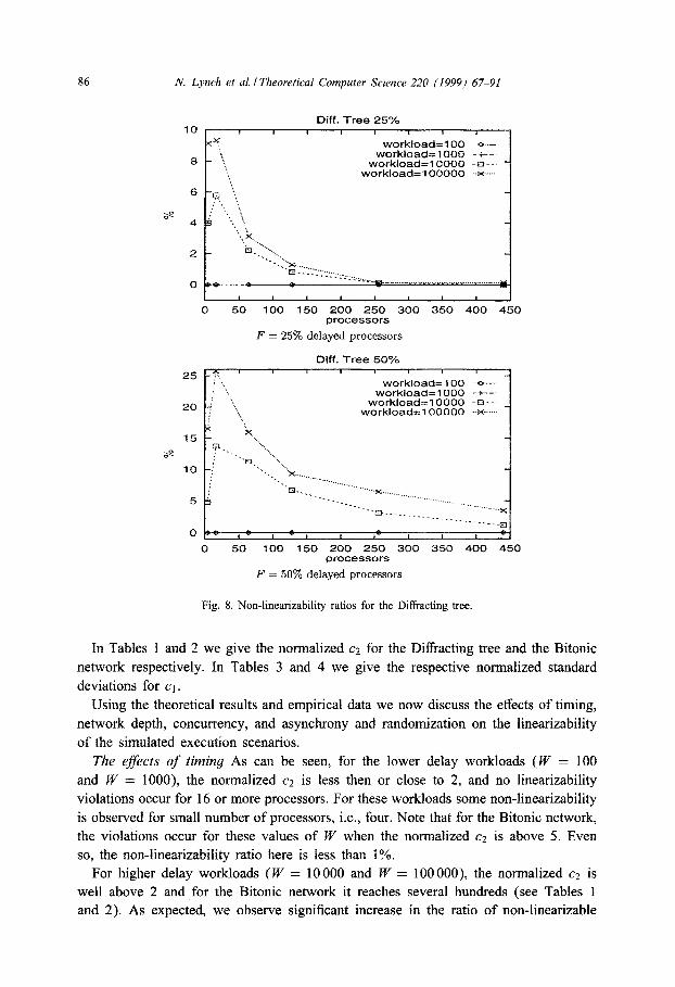
The main results are presented in Fig. 8 for the Diffracting tree and Fig. 9 for the
Bitonic network. The charts show the non-linearizability ratio as the function of the
number of processors P. Each figure contains two charts, one showing the results with
25% delayed processors and the other with 50% delayed processors.
86 N. Lynch er al. I Theoretical Computer Science 220 (1999) 67-91
Diff. Tree 25%
0 50 100 150 200 250 300 350 400 450 processors
F = 25% delayed processors
Diff. Tree 50%
workload=1 00000 --x.---
50 100 150 200 250 300 350 400 450 processors
F = 50% delayed processors
Fig. 8. Non-linearizability ratios for the Diffracting tree.
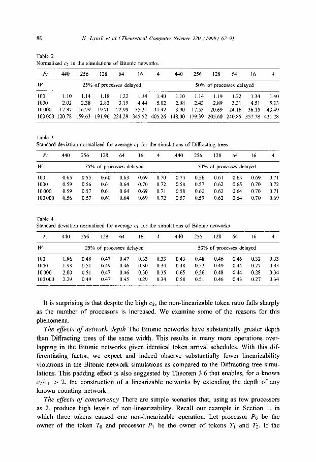
In Tables 1 and 2 we give the normalized c2 for the Diffracting tree and the Bitonic
network respectively. In Tables 3 and 4 we give the respective normalized standard
deviations for ct.
Using the theoretical results and empirical data we now discuss the effects of timing,
network depth, concurrency, and asynchrony and randomization on the linearizability
of the simulated execution scenarios.
The e&f&s of timing As can be seen, for the lower delay workloads (IV = 100
and W = lOOO), the normalized c2 is less then or close to 2, and no linearizability
violations occur for 16 or more processors. For these workloads some non-linearizability
is observed for small number of processors, i.e., four. Note that for the Bitonic network,
the violations occur for these values of IV when the normalized c2 is above 5. Even
so, the non-linea~zability ratio here is less than 1%.
For higher delay workloads ( W = 10 000 and W = 100 000), the normalized c2 is
well above 2 and for the Bitonic network it reaches several hundreds (see Tables 1
and 2). As expected, we observe significant increase in the ratio of non-linearizable

N. Lynch et al. I Theoretical Computer Science 220 (1999) 67-91 87
14
12
10
a S
6
4
2
0
Bitonic Net 25%
31
I I I I I , I I
100 150 200 250 300 350 400 450 processors
F = 25% delayed processors
Bitonic Net 50%
workload=1 00 -+- workload=1 000 -+-.
workload=1 0000 workload=1 00000 --w.-
0 50 100 150 200 250 300 350 400 450 processors
F = 50% delayed processors
Fig. 9. Non-linearizability ratios for the Bitonic network
Table 1
Normalized q in the simulations of Diffracting trees
P: 440 256 128 64 16 4 440 256 128 64 16 4
W 25% of processes delayed 50% of processes delayed
100 1.10 1.10 1.09 1.08 1.08 1.08 1.10 1.10 1.09 1.08 1.08 1.08
1000 2.02 2.01 1.88 1.77 1.71 1 .I3 2.04 2.00 1.86 1 .I5 1 .I6 1.72
10000 11.28 10.78 9.43 8.43 8.76 8.35 11.16 10.16 8.81 8.09 8.49 8.46
100000 105.54 98.72 84.48 74.61 78.30 74.34 103.51 90.12 76.44 70.14 76.38 81.14
operations. For the Diffracting tree the ratios peak at about 26% for 16 processors 50%
of which incur delays of W = 100 000. For the Bitonic network the peak ratio is about
12% for the same parameters. Substantially lower peak non-linearizable ratios, of 10%
and 5% respectively, are observed for F = 25% and 16 processors.
88 N. Lynch et ul. I Theoretical Computer Science 220 (1999) 67-91
Table 2
Normalized q in the simulations of Bitonic networks
P: 440 256 128 64 16 4 440 256 128 64 16 4
W 25% of processes delayed 50% of processes delayed
100 1.10 1.14 1.18 1.22 1.34 1.40 1.10 1.14 1.19 1.22 1.34 1.40
1000 2.02 2.38 2.83 3.19 4.44 5.02 2.08 2.43 2.89 3.31 4.5 I 5.13 10000 12.37 16.29 19.70 22.99 35.31 41.42 13.90 17.53 20.69 24.16 36.15 43.49
100000 120.78 159.63 191.96 224.29 345.52 405.26 148.00 179.39 205.60 240.85 357.78 431.28
Table 3
Standard deviation normalized for average cl for the simulations of Diffracting trees
P: 440 256 128 64 16 4 440 256 128 64 16 4
W 25% of processes delayed 50% of processes delayed
100 0.65 0.55 0.60 0.63 0.69 0.70 0.73 0.56 0.61 0.63 0.69 0.71
1000 0.59 0.56 0.61 0.64 0.70 0.72 0.58 0.57 0.62 0.65 0.70 0.72
10000 0.59 0.57 0.61 0.64 0.69 0.71 0.58 0.60 0.62 0.64 0.70 0.71
100000 0.56 0.57 0.61 0.64 0.69 0.72 0.57 0.59 0.62 0.64 0.70 0.69
Table 4
Standard deviation normalized for average cl for the simulations of Bitonic networks
P: 440 256 128 64 16 4 440 256 128 64 16 4
W 25% of processes delayed 50% of processes delayed
100 1.86 0.48 0.47 0.47 0.33 0.33 0.43 0.48 0.46 0.46 0.32 0.33
1000 1.93 0.51 0.49 0.46 0.30 0.34 0.48 0.52 0.49 0.44 0.27 0.33
10000 2.00 0.5 1 0.47 0.46 0.30 0.35 0.65 0.56 0.48 0.44 0.28 0.34
100 000 2.29 0.49 0.47 0.45 0.29 0.34 0.58 0.51 0.46 0.43 0.27 0.34
It is surprising is that despite the high ~2, the non-linearizable token ratio falls sharply
as the number of processors is increased. We examine some of the reasons for this
phenomena.
The ejjixts of network depth The Bitonic networks have substantially greater depth
than Diffracting trees of the same width. This results in many more operations over-
lapping in the Bitonic networks given identical token arrival schedules. With this dif-
ferentiating factor, we expect and indeed observe substantially fewer linearizability
violations in the Bitonic network simulations as compared to the Diffracting tree simu-
lations. This padding effect is also suggested by Theorem 3.6 that enables, for a known
c2Ict > 2, the construction of a linearizable networks by extending the depth of any
known counting network.
The efsects of concurrency There are simple scenarios that, using as few processors
as 2, produce high levels of non-linearizability. Recall our example in Section 1, in
which three tokens caused one non-linearizable operation. Let processor PO be the
owner of the token TO and processor PI be the owner of tokens Tl and T2. If the

N. Lynch et ul. I Theoretical Computer Science 220 (1999) 67-91 89
token To is very slow, so that it does not exit the network for a long time, then any
sequence of tokens Ti generated by PO will have each of its even-numbered tokens
Tlj return lower counter values than its odd-numbered tokens Tzj-1 for j > 0. This is
because the even- and odd-numbered tokens traverse the network sequentially. If there
were three processors, such that T2j is concurrent with T,- 1, then the there would be
no nonlinearizable operations.
Although far from a complete characterization, the above observation of linearizabil-
ity versus concurrency provides intuition for why there is a dramatic reduction, at high
concurrency, in the number of non-linearizable operations for both the Diffracting tree
and the Bitonic network.
Of course the counting network approach is optimized for high concurrency, so it
is not surprising that deploying counting networks in low-concurrency setting has its
drawbacks. For few processors, there are more efficient and linearizable solutions [14].
The e&f&s of asynchrony and randomization We also tested the linearizability of
our implementation when either all or no tokens were delayed, i.e., the cases of F = 0% and F = loo%, and/or when the additional delays were eliminated, i.e., W = 0. In none
of these simulation were there any non-linearizable operations. Although not surprising _ these scenarios create timing schedules close to those of an implementation that is
synchronous - we performed these simulations for completeness.
In another simulation scenario we forced every token to wait a random number
of cycles between 0 and W. Again, the simulation was observed to be completely
linearizable. Randomization apparently has attenuating effect that prevents consistent
accumulation of timing discrepancies by faster or slower tokens.
6. Conclusions and discussion
Our paper studies the effects of timing on the linearizability of uniform counting
networks. Our results were recently extended and generalized by Mavronicolas et al.
[20], to include non-uniform networks. For a given network G, let d be the maximum
path length from inputs to outputs, and s be the shortest such path. They show that a
counting network is linearizable if ~/et <2sld (for uniform networks s = d, and the
linearizability requirement reduces to the cz/ct 62 shown in Section 3). Furthermore,
they introduce the powerful notion of an influence radius of a graph G, iradc;, as the
length of the maximum common subpath of any two maximal paths from an internal
balancer to any two outputs, and show that a network is not linearizable if Q/C, >
d/iradc + 1 (for uniform networks iradc = d, and linearizability is violated when
cz/ct > 2 as we show here).
We have considered 1ocaZ timing characteristics at balancers. The linearizablility
question can also be posed in terms of global timing characteristics, i.e., in terms of the
minimum and maximum time it takes a token to traverse the entire network and without
the restriction on the time to traverse each individual balancer. Our examination of
Counting trees and Bitonic networks shows that violations of required local conditions

90 N. Lynch et al. I Theoretical Computer Science 220 (1999) 67-91
lead to non-linearizable executions (this is also shown for general networks in [20]).
In these executions we use tokens that traverse a network at the fastest and the slowest
possible paces. The fast tokens “bypass” the slow tokens only at the exits. Therefore
even if the required conditions are global, our scenarios still yield non-linearizable
executions.
There are many other variations of the timing model which one may investigate.
However, we feel the most interesting direction to follow at this time is the character-
ization of applications that do not have an absolute requirement for linearizability, that
is, ones requiring that only a given fraction of the operations be linearizable.
Acknowledgements
The authors thank Maurice Herlihy for insightful comments, and Marios Mavroni-
colas and the anonymous referees for several helpful suggestions.
References
[l] A. Agarwal, R. Bianchini, D. Chaiken, D.K.K. Johnson, J. Kubiatowicz, B.-H. Lim, K. MacKenzie, D.
Yeung, The MIT Alewife Machine: architecture and Performance, in: 22nd Intemat. Symp. on Computer
Architecture, Santa Margherita Ligure, Italy, June 1995, pp. 2-13.
[2] E. Aharonson, H. Attiya, Counting networks with arbitrary fan out, D&rib. Comput. 8 (4) (1995)
163-169. Also: Technical Report 679, The Technion, June 1991. Earlier version in [2].
[3] B. Aiello, R. Venkatesan, M. Yung, Coins, weights and contention in balancing Networks, in: Proc.
13th Amm. ACM Symp. on Principles of Distributed Computing, Los Angeles, CA, August 1994, pp.
193-214.
[4] J. Aspnes, M. Herlihy, N. Shavit, Counting networks, J. ACM 41 (5) (1994) 102&1048. Earlier
version in: Proc. 23rd ACM Amm. Symp. on Theory of Computing, May 1991, pp. 348-358. Also,
MIT Technical Report MITILCSITM-45 1, June 1991. [5] H. Attiya, C. Dwork, N. Lynch, L. Stockmeyer, Bounds on the time to reach agreement in the presence
of timing uncertainty, J. ACM 41 (1) (1994) 122-152. [6] H. Attiya, N. Lynch, N. Shavit, Are wait-free Algorithms Fast? J. ACM 41 (4) (1994) 7255763.
[7] K.E. Batcher, Sorting networks and their applications, Proc. AFIPS Spring Joint Computer Conf., 1968,
pp. 307-314. [8] E.A. Brewer, C.N. Dellarocas, A. Colbrook, W.E. Weihl, Proteus: a high-performance parallel-
architecture simulator, Technical Report MITILCSITR-5 16, MIT Laboratory for Computer Science,
September 1991.
[9] C. Busch, M. Mavronicolas, A Combinatorial Treatment of Balancing Networks, in: Proc. 13th Annu.
ACM Symp. on Principles of Distributed Computing, Los Angeles, CA, August 1994, pp. 206-215. [lo] C. Busch, M. Mavronicolas, New bounds on depth and contention for counting networks, Preprint,
Univ. of Cyprus, October 1995. [ll] T.H. Cormen, C.E. Leiserson, R.L. Rivest, Introduction to Algorithms, MIT Press/McGraw-Hill,
Cambridge MA/New York, 1990. [12] E.W. Felten, A. LaMarca, R. Ladner, Building counting networks from larger balancers, Technical
Report TR-93-04-09, University of Washington, April 1993. [13] J.R. Goodman, M.K. Vernon, P.J. Woest, Efficient synchronization primitives for large-scale cache-
coherent multiprocessors, in: Proc. 3rd Intemat. Conf. on Architectural Support for Programming
Languages and Operating Systems, Boston, Ma, April 1989, pp. 64-75. [14] M. Herlihy, B.H. Lim, N. Shavit, Scalable concurrent counting, ACM Trans. Comput. Systems 13
(4) (1995) 343-364. Earlier version in: Proc. 3rd Amm. ASM Symp. on Parallel Algorithms and
Architectures (SPAA), San Diego, CA, July 1992, pp. 219-227. Full version available as DEC TR.

N. Lynch et al. I Theoretical Computer Science 220 (1999) 67-91 91
[15] M. Herlihy, N. Shavit, 0. Waarts, Low contention linearizable counting, in: Proc. 32nd Amm. Symp. on
Foundations of Computer Science (FOCS), San Juan, Puerto Rico, October 1991, pp. 526535. IEEE.
Detailed version with empirical results appeared as MIT Technical Memo MIT/‘LCS/TM-459, November
1991. [16] M.P. Herlihy, J.M. Wing, Linearizability: a correctness condition for concurrent objects, ACM Trans.
Programming Languages Systems 12 (3) (1990) 463492.
[17] M. Klugerman, C.G. Plaxton, Small-depth counting networks, PhD thesis, MIT, Cambridge, MA 02139,
1994.
[18] M. Klugerman, C.G. Plaxton, Small-depth counting networks, in: Proc. 24th ACM Symp. on Theory of
Computing (STOC), 1992, pp. 417428.
[ 191 L. Lamport, How to make a multiprocessor computer that correctly executes multiprocess programs,
IEEE Trans. Computers C-28 (9) (1979).
[20] M. Mavronicolas, M. Papatriantafilou and P. Tsigas, The Impact of timing on linearizability in counting
networks, 1997 1 lth Intemat. Parallel Processing Symp., Geneva, Switzerland, to appear.
[21] J.M. Mellor-Crummey, M.L. Scott, Algorithms for scalable synchronization on shared-memory
multiprocessors, ACM Trans. Comput Systems 9 (I) (1991) 21-65. Earlier version published as TR
342, University of Rochester, Computer Science Department, April 1990, and COMP TR90-1 14, Center
for Research on Parallel Computation, Rice UNIV, May 1990.
[22] C.H. Papadimitriou, The serializability of concurrent database updates, J. ACM 26 (4) (1979) 63 1653.
[23] N. Shavit, D. Touitou, Elimination trees and the construction of pools and stacks, in: SPAA’95: 7th
Annu. ACM Symp. on Parallel Algorithms and Architectures, Santa Barbara, Ca, July 1995, pp. 54-63.
Also, Tel-Aviv University Technical Report, January 1995.
[24] N. Shavit, A. Zemach, Diffracting trees, ACM Trans. Comput. Systems 14 (4) (1996) 385428.
[25] P.M.B. Vitanyi, Distributed elections in an archimedean ring of processors, in: Proc. 16th ACM Symp.
on Theory of Computing, 1984, pp. 542-547.