Timing Analysis - uni-saarland.de · Structure of the Lecture 1. Introduction 2. Static timing analysis 1. the problem 2. our approach 3. the success 4. tool architecture

Timing Analysis - timing guarantees for hard real-time systems-

Reinhard Wilhelm

Saarland University Saarbrücken

TexPoint fonts used in EMF. Read the TexPoint manual before you delete this box.: AAAAA

Structure of the Lecture 1.  Introduction 2.  Static timing analysis

1.  the problem 2.  our approach 3.  the success 4.  tool architecture

3.  Cache analysis 4.  Pipeline analysis 5.  Value analysis 6.  Worst-case path determination ----------------------------------------------------------- 1.  Timing Predictability

•  caches •  non-cache-like devices •  future architectures

2.  Conclusion

Industrial Needs Hard real-time systems, often in safety-critical

applications abound –  Aeronautics, automotive, train industries, manufacturing control

Wing vibration of airplane, sensing every 5 mSec

Sideairbag in car, Reaction in <10 mSec

crankshaft-synchronous tasks have very tight deadlines, ~45uS

Hard Real-Time Systems

•  Embedded controllers are expected to finish their tasks reliably within time bounds.

•  Task scheduling must be performed •  Essential: upper bound on the execution times of

all tasks statically known •  Commonly called the Worst-Case Execution Time

(WCET) •  Analogously, Best-Case Execution Time (BCET)

Static Timing Analysis

Embedded controllers are expected to finish their tasks reliably within time bounds.

The problem: Given 1.  a software to produce some reaction, 2.  a hardware platform, on which to execute the

software, 3.  required reaction time. Derive: a guarantee for timeliness.

Timing Analysis

•  provides parameters for schedulability analysis:

•  Execution time, Ci, of tasks, and if that is impossible,

•  upper bounds and maybe also lower bounds on execution times of tasks, often called Worst-Case Execution Times (WCET) and Best-Case Execution Times (BCET).

What does Execution Time Depend on?

•  the input – this has always been so and will remain so,

•  the initial execution state of the platform – this is (relatively) new,

•  interferences from the environment – this depends on whether the system design admits it (preemptive scheduling, interrupts).

Caused by caches, pipelines, speculation etc.

Explosion of the space of inputs and initial states

⇒  no exhaustive approaches feasible.

“external” interference as seen from analyzed task

Variability of Execution Times LOAD r2, _a!

LOAD r1, _b!

ADD r3,r2,r1!

0

50

100

150

200

250

300

350

Best Case Worst Case

Execution Time (Clock Cycles)

Clock Cycles

PPC 755

x = a + b;

In most cases, execution will be fast. So, assuming the worst case is safe, but very pessimistic!

Notions in Timing Analysis Hard or

impossible to determine

Determine upper bounds

instead

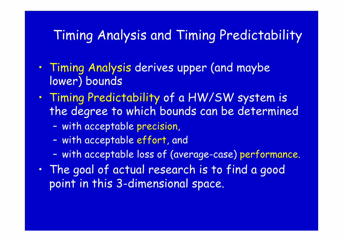
Timing Analysis and Timing Predictability

•  Timing Analysis derives upper (and maybe lower) bounds

•  Timing Predictability of a HW/SW system is the degree to which bounds can be determined –  with acceptable precision, –  with acceptable effort, and –  with acceptable loss of (average-case) performance.

•  The goal of actual research is to find a good point in this 3-dimensional space.

Timing Analysis

•  Sounds methods determine upper bounds for all execution times,

•  can be seen as the search for a longest path,

–  through different types of graphs, –  through a huge space of paths.

1.  I will show how this huge state space originates.

2.  How and how far we can cope with this huge state space.

Architecture

(constant execution

times)

Timing Analysis – the Search Space •  all control-flow paths (through the

binary executable) – depending on the possible inputs.

•  Feasible as search for a longest path if – Iteration and recursion are bounded, Execution time of instructions are (positive) constants.

•  Elegant method: Timing Schemata (Shaw’89, Puschner/Koza’89) – inductive calculation of upper bounds.

Software

Input

ub (if b then S1 else S2) := ub (b) + max (ub (S1), ub (S2))

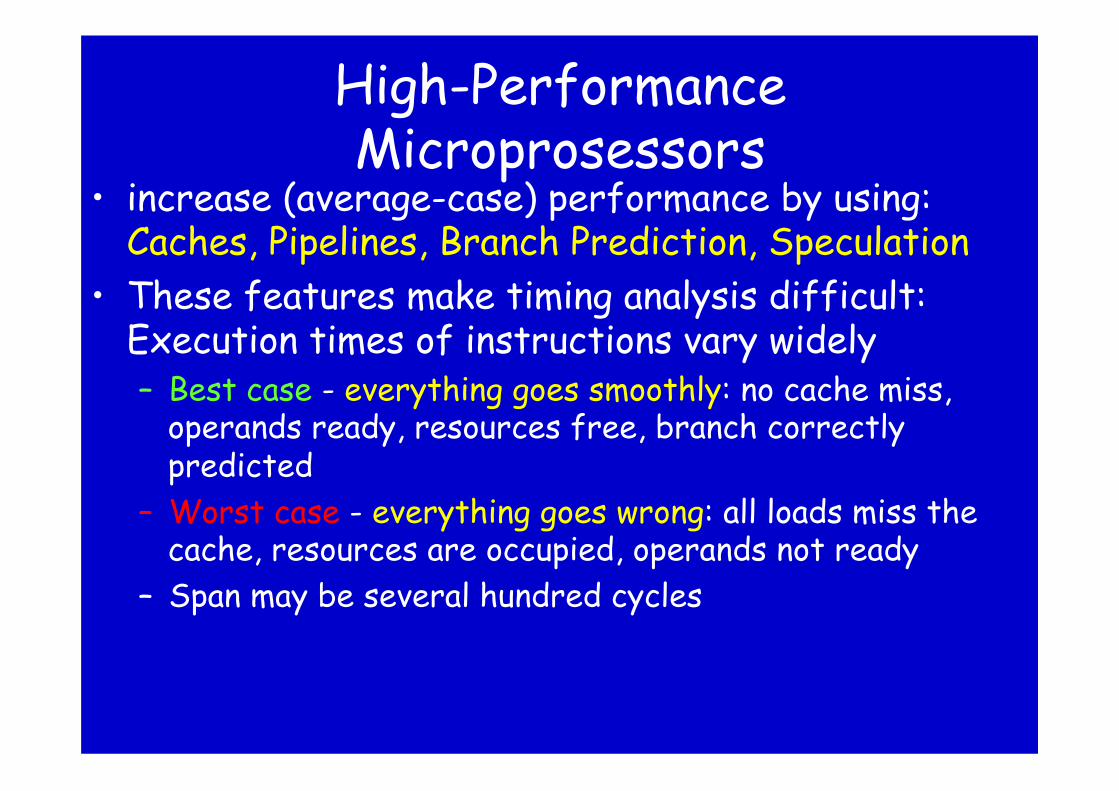
High-Performance Microprosessors

•  increase (average-case) performance by using: Caches, Pipelines, Branch Prediction, Speculation

•  These features make timing analysis difficult: Execution times of instructions vary widely –  Best case - everything goes smoothly: no cache miss,

operands ready, resources free, branch correctly predicted

–  Worst case - everything goes wrong: all loads miss the cache, resources are occupied, operands not ready

–  Span may be several hundred cycles

State-dependent Execution Times

•  Execution time of an instruction is a function of the execution state è timing schemata no more applicable.

•  Execution state results from the execution history.

semantics state: values of variables

execution state: occupancy of resources

state

Architecture

Timing Analysis – the Search Space with State-dependent Execution Times

•  all control-flow paths – depending on the possible inputs

•  all paths through the architecture for potential initial states

Software

Input

initial state

mul rD, rA, rB execution states for paths reaching this program point

instruction in I-cache

instruction not in I-cache

1

bus occupied

bus not occupied

small operands

large operands

1

4 ≥ 40

Architecture

Timing Analysis – the Search Space with out-of-order execution



•  including different schedules for instruction sequences

Software

Input

initial state

Architecture

Timing Analysis – the Search Space with multi-threading



•  including different schedules for instruction sequences

•  including different interleavings of accesses to shared resources

Software

Input

initial state

Why Exhaustive Exploration? •  Naive attempt: follow local worst-case transitions

only •  Unsound in the presence of Timing Anomalies:

A path starting with a local worst case may have a lower overall execution time, Ex.: a cache miss preventing a branch mis-prediction

•  Caused by the interference between processor components: Ex.: cache hit/miss influences branch prediction; branch prediction causes prefetching; prefetching pollutes the I-cache.

First reference to Timing Anomalies

“the slower ones will later be fast“ The times they are a’changing, 1963

State Space Explosion in Timing Analysis

constant execution times

state-dependent execution times

out-of-order execution

preemptive scheduling

concurrency + shared resources

years + methods ~1995 ~2000 2010+

Timing schemata Static analysis ???

Caches, pipelines,

speculation: combined cache and

pipeline analysis

Superscalar processors:

interleavings of all schedules

Multi-core with

shared resources:

interleavings of several threads

AbsInt‘s WCET Analyzer aiT IST Project DAEDALUS final

review report: "The AbsInt tool is probably the best of its kind in the world and it is justified to consider this result as a breakthrough.”

Several time-critical subsystems of the Airbus A380 have been certified using aiT; aiT is the only validated tool for these applications.

Tremendous Progress during the past 15 Years

1995 2002 2005

over

-est

imat

ion

20-30% 15%

30-50%

4

25

60

200

cach

e-m

iss p

enal

ty

Lim et al. Thesing et al. Souyris et al.

The explosion of penalties has been compensated by the improvement of the analyses!

10%

25%

Tool Architecture

Abstract Interpretations

Abstract Interpretation Integer Linear Programming

combined cache and pipeline

analysis

determines enclosing intervals

for the values in registers and local

variables

determines loop bounds determines

infeasible paths

derives invariants about architectural execution states,

computes bounds on execution times of basic blocks

determines a worst-case path and an

upper bound

High-Level Requirements for Timing Analysis

•  Upper bounds must be safe, i.e. not underestimated

•  Upper bounds should be tight, i.e. not far away from real execution times

•  Analogous for lower bounds •  Analysis effort must be tolerable

Note: all analyzed programs are terminating, loop bounds need to be known ⇒

no decidability problem, but a complexity problem!

Timing Accidents and Penalties Timing Accident – cause for an increase

of the execution time of an instruction Timing Penalty – the associated increase •  Types of timing accidents

–  Cache misses –  Pipeline stalls –  Branch mispredictions –  Bus collisions – Memory refresh of DRAM –  TLB miss

Execution Time is History-Sensitive Contribution of the execution of an instruction to

a program‘s execution time •  depends on the execution state, e.g. the time

for a memory access depends on the cache state

•  the execution state depends on the execution history

•  needed: an invariant about the set of execution states produced by all executions reaching a program point.

•  We use abstract interpretation to compute these invariants.

Deriving Run-Time Guarantees

•  Our method and tool, aiT, derives Safety Properties from these invariants : Certain timing accidents will never happen. Example: At program point p, instruction fetch will never cause a cache miss.

•  The more accidents excluded, the lower the upper bound.

Murphy’s invariant

Fastest Variance of execution times Slowest

Abstract Interpretation in Timing Analysis •  Abstract interpretation statically analyzes a

program for a given property without executing it. •  Derived properties therefore hold for all

executions. •  It is based on the semantics of the analyzed

language. •  A semantics of a programming language that talks

about time needs to incorporate the execution platform!

•  Static timing analysis is thus based on such a semantics.

The Architectural Abstraction inside the Timing Analyzer

Timing analyzer

Architectural abstractions

Cache Abstraction

Pipeline Abstraction

Value Analysis, Control-Flow Analysis, Loop-Bound Analysis

abstractions of the processor’s arithmetic

Abstract Interpretation in Timing Analysis

Determines •  invariants about the values of variables

(in registers, on the stack) –  to compute loop bounds –  to eliminate infeasible paths –  to determine effective memory addresses

•  invariants on architectural execution state –  Cache contents ⇒ predict hits & misses –  Pipeline states ⇒ predict or exclude pipeline stalls

The Story in Detail

Tool Architecture

Value Analysis •  Motivation:

–  Provide access information to data-cache/pipeline analysis

–  Detect infeasible paths –  Derive loop bounds

•  Method: calculate intervals at all program points, i.e. lower and upper bounds for the set of possible values occurring in the machine program (addresses, register contents, local and global variables) (Cousot/Halbwachs78)

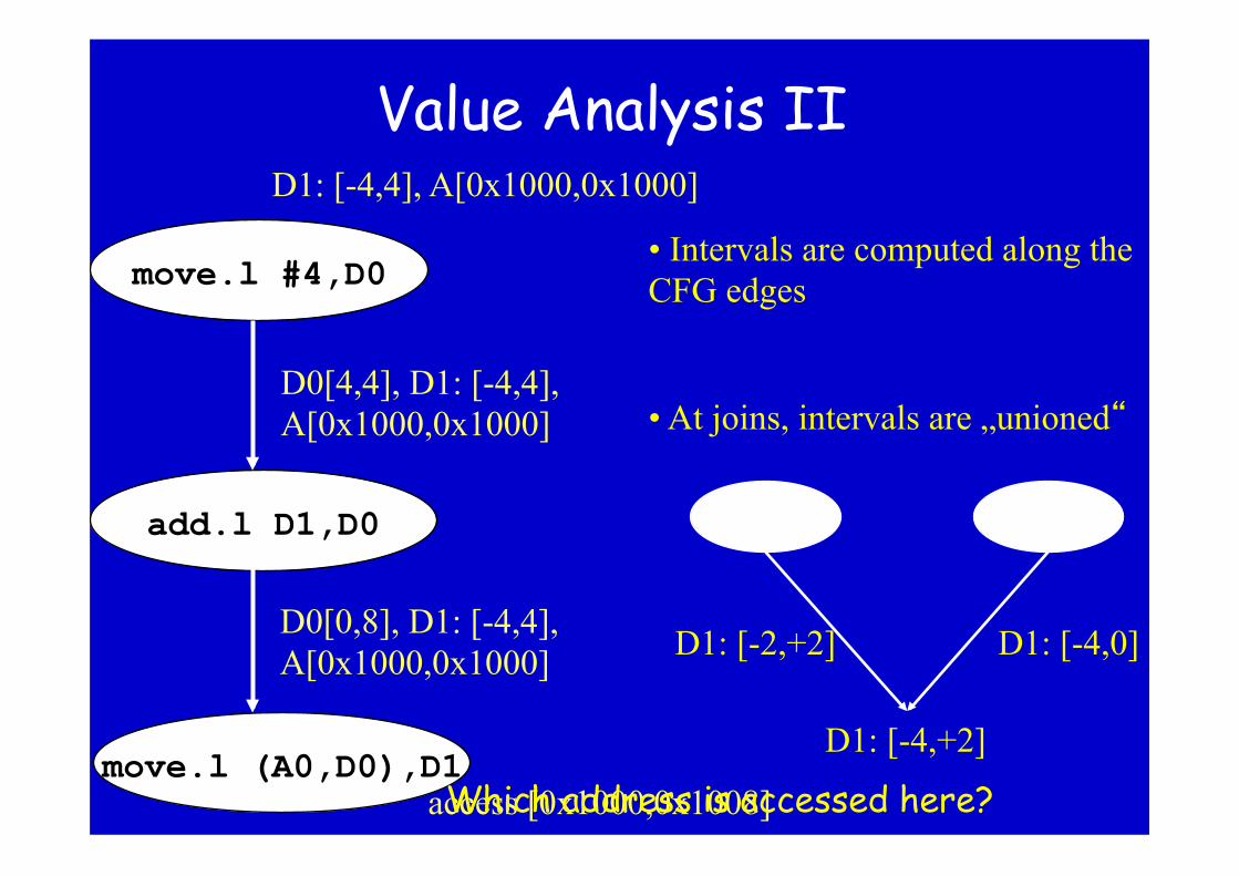
Value Analysis II

•  Intervals are computed along the CFG edges

•  At joins, intervals are „unioned“

D1: [-2,+2] D1: [-4,0]

D1: [-4,+2]

move.l #4,D0

add.l D1,D0

move.l (A0,D0),D1

D1: [-4,4], A[0x1000,0x1000]

D0[4,4], D1: [-4,4], A[0x1000,0x1000]

D0[0,8], D1: [-4,4], A[0x1000,0x1000]

access [0x1000,0x1008] Which address is accessed here?

Value Analysis (Airbus Benchmark) Task Unreached Exact Good Unknown Time [s]

1 8% 86% 4% 2% 47 2 8% 86% 4% 2% 17 3 7% 86% 4% 3% 22 4 13% 79% 5% 3% 16 5 6% 88% 4% 2% 36 6 9% 84% 5% 2% 16 7 9% 84% 5% 2% 26 8 10% 83% 4% 3% 14 9 6% 89% 3% 2% 34

10 10% 84% 4% 2% 17 11 7% 85% 5% 3% 22 12 10% 82% 5% 3% 14

1Ghz Athlon, Memory usage <= 20MB

Good means less than 16 cache lines

Tool Architecture

Caches

Tool Architecture



Caches

Caches: Small & Fast Memory on Chip

•  Bridge speed gap between CPU and RAM •  Caches work well in the average case:

– Programs access data locally (many hits) – Programs reuse items (instructions, data) –  Access patterns are distributed evenly across

the cache •  Cache performance has a strong influence on

system performance!

Caches: How they work CPU: read/write at memory address a,

–  sends a request for a to bus Cases: •  Hit:

–  Block m containing a in the cache: request served in the next cycle

•  Miss: –  Block m not in the cache:

m is transferred from main memory to the cache, m may replace some block in the cache, request for a is served asap while transfer still continues

a

m

Replacement Strategies

•  Several replacement strategies: LRU, PLRU, FIFO,...

determine which line to replace when a memory block is to be loaded into a full cache (set)

LRU Strategy •  Each cache set has its own replacement logic =>

Cache sets are independent: Everything explained in terms of one set

•  LRU-Replacement Strategy: –  Replace the block that has been Least Recently Used –  Modeled by Ages

•  Example: 4-way set associative cache age 0 1 2 3

m0 m1 Access m4 (miss) m4 m2

m1 Access m1 (hit) m0 m4 m2 m1 m5 Access m5 (miss) m4 m0

m0 m1 m2 m3

Cache Analysis How to statically precompute cache contents: •  Must Analysis:

For each program point (and context), find out which blocks are in the cache → prediction of cache hits

•  May Analysis: For each program point (and context), find out which blocks may be in the cache Complement says what is not in the cache → prediction of cache misses

•  In the following, we consider must analysis until otherwise stated.

(Must) Cache Analysis •  Consider one instruction in

the program. •  There may be many paths

leading to this instruction. •  How can we compute

whether a will always be in cache independently of which path execution takes?

load a

Question: Is the access to a always a cache hit?

Determine Cache-Information (abstract cache states) at each Program Point

{a, b} {x}

youngest age - 0 oldest age - 3

Interpretation of this cache information: describes the set of all concrete cache states in which x, a, and b occur •  x with an age not older than 1 •  a and b with an age not older than 2, Cache information contains 1.  only memory blocks guaranteed to be in cache. 2.  they are associated with their maximal age.

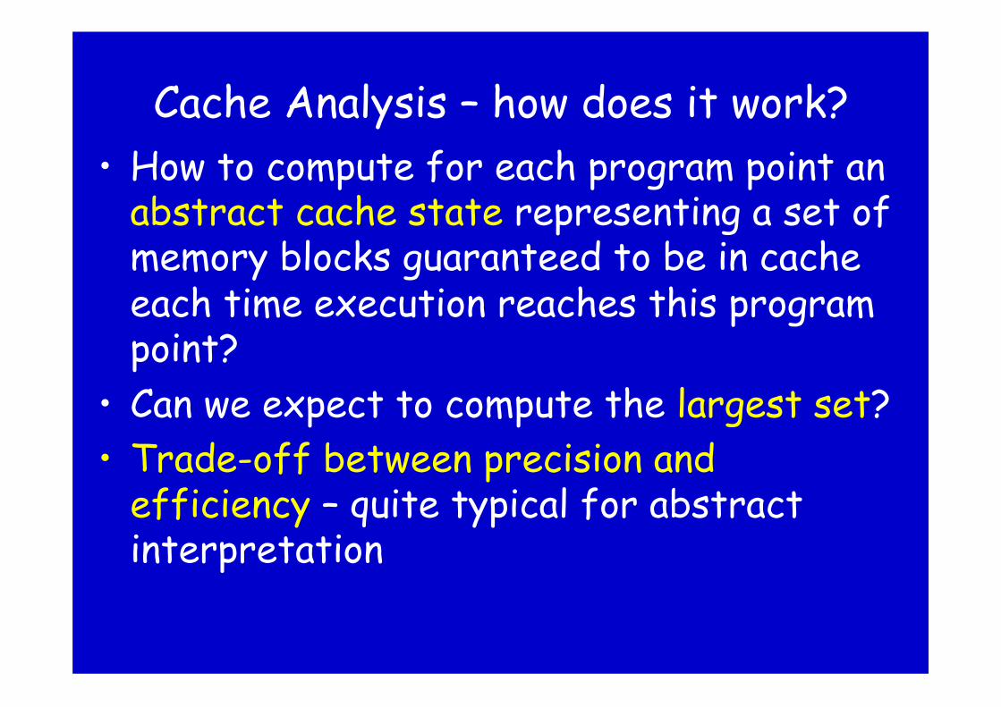
Cache Analysis – how does it work? •  How to compute for each program point an

abstract cache state representing a set of memory blocks guaranteed to be in cache each time execution reaches this program point?

•  Can we expect to compute the largest set? •  Trade-off between precision and

efficiency – quite typical for abstract interpretation

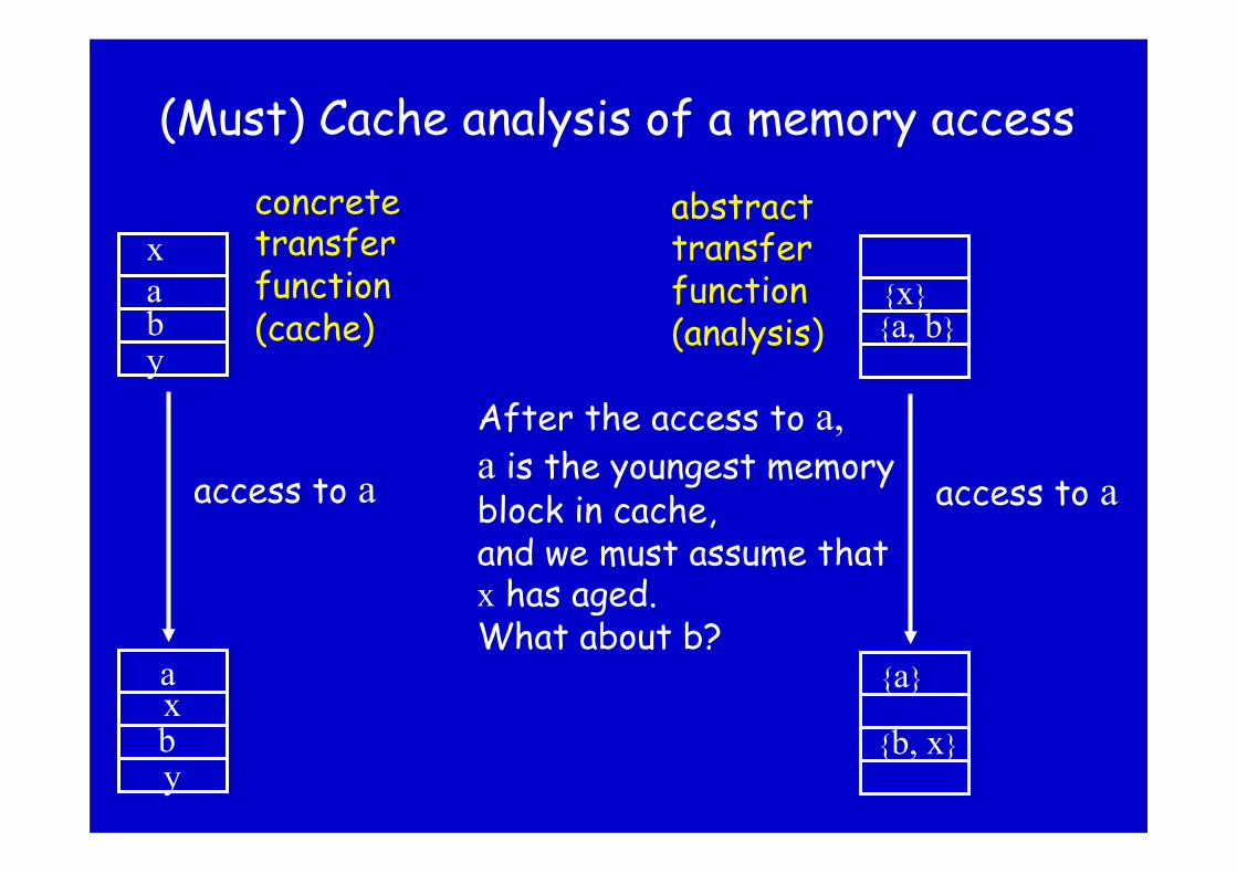
(Must) Cache analysis of a memory access

{a, b} {x}

access to a

{b, x}

{a}

After the access to a, a is the youngest memory block in cache, and we must assume that x has aged. What about b?

b a

access to a

b

a

x

y

y

x

concrete transfer function (cache)

abstract transfer function (analysis)

Combining Cache Information •  Consider two control-flow paths to a program point:

–  for one, prediction says, set of memory blocks S1 in cache, –  for the other, the set of memory blocks S2. –  Cache analysis should not predict more than S1 ∩ S2 after the merge of paths. –  the elements in the intersection should have their maximal age from S1 and S2.

•  Suggests the following method: Compute cache information along all paths to a program point and calculate their intersection – but too many paths!

•  More efficient method: –  combine cache information on the way, –  iterate until least fixpoint is reached.

•  There is a risk of losing precision, not in case of distributive transfer functions.

What happens when control-paths merge?

{ a } { }

{ c, f } { d }

{ c } { e } { a } { d }

{ } { }

{ a, c } { d }

“intersection + maximal age”

We can guarantee this content on this path.

We can guarantee

this content on this path.

Which content can we

guarantee on this path?

combine cache information at each control-flow merge point

Must-Cache and May-Cache- Information

•  The presented cache analysis is a Must Analysis. It determines safe information about cache hits. Each predicted cache hit reduces the upper bound.

•  We can also perform a May Analysis. It determines safe information about cache misses Each predicted cache miss increases the lower bound.

(May) Cache analysis of a memory access

{a, b} {x}

access to a

{x}

{a}

Why? After the access to a a is the youngest memory block in cache, and we must assume that x, y and b have aged.

{b, z}

{y}

{z}

{y}

Cache Analysis: Join (may) { a } { }

{ c, f } { d }

{ c } { e } { a } { d }

{ a,c } { e} { f } { d }

“union + minimal age”

Join (may)

Result of the Cache Analyses

Category Abb. Meaning

always hit ah The memory reference will

always result in a cache hit.

always miss am The memory reference will

always result in a cache miss.

not classified nc The memory reference could

neither be classified as ah

nor am.

Categorization of memory references

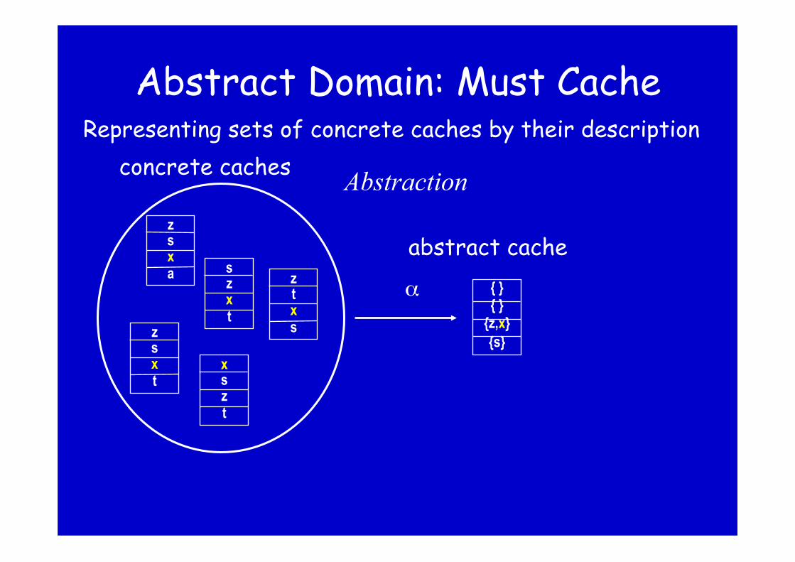
Abstract Domain: Must Cache

z s x a

x s z t

z s x t

s z x t

z t x s

α

Abstraction

Representing sets of concrete caches by their description concrete caches

{ } { }

{z,x} {s}

abstract cache

Abstract Domain: Must Cache

{ } { }

{z,x} {s}

γ

Concretization

{ s∈ { z, x ∈

Sets of concrete caches described by an abstract cache

remaining line filled up with any other block

concrete caches

abstract cache

over-approximation!

Abstract Domain: May Cache

z s x a

x s z t

z s x t

s z x t

z t x s

{z ,s, x} { t } { }

{ a }

α

Abstraction

abstract cache

concrete caches

Abstract Domain: May Cache

γ

Concretization

{z,s,x} { t } { }

{ a }

abstract may-caches say what definitely is not in cache and what the minimal age of those is that may be in cache.

∈{z,s,x} ∈{z,s,x,t} ∈{z,s,x,t} ∈{z,s,x,t,a}

concrete caches

abstract cache

Cache Analysis Over-approximation of the Collecting Semantics

the semantics set of all cache states for each program point

determines

“cache” semantics set of cache states for each program point

determines

abstract semantics abstract cache states for each program point

determines

conc

Collecting semantics collects at each program point all states that any execution may encounter

there.

reduces the program to the sequence of memory references

Complete Lattices: The Mathematics of Semantic Domains

Bottom element ?

Top element >

a v b Information order v

Convention: b more precise than a

a b t Join operator t combines information

Set A of elements Relation between t and v: a v b iff a t b = b

(A, v, t, u, >, ?)

Lattice for Must Cache

•  Set A of elements •  Information order v •  Join operator t •  Top element > •  Bottom element ?

{ } { }

{z,x} {s}

Abstract cache states:

Upper bounds on the age of memory blocks guaranteed to be in cache

“young”

“old”

Age

Lattice for Must Cache


{ } { } {z} {s}

{ } {z} {x} {s}

v “young”

“old”

Age

Better precision:

more elements in the cache or with younger age.

NB. The more precise abstract cache represents less concrete cache states!

Lattice: Must Cache


{ a } { }

{ c, f } { d }

{ c } { e } { a } { d }

{ } { }

{ a, c } { d }

t

Form the intersection and

associate the elements with

the maximum of their ages

“young”

“old”

Age

Lattice: Must Cache


{ } { } { } { }

“young”

“old”

Age

No information:

All caches possible

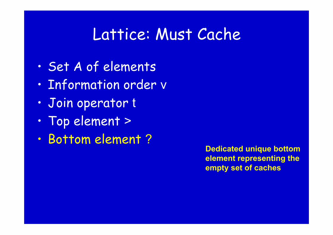
Lattice: Must Cache


Dedicated unique bottom element representing the empty set of caches

Galois connection – Relating Semantic Domains

•  Lattices C, A •  two monotone functions ® and ° •  Abstraction: ®: C → A •  Concretization °: A → C •  (®,°) is a Galois connection

if and only if ° • ® wC idC and ® • ° vA idA

Switching safely between concrete and abstract domains, possibly losing precision

Abstract Domain Must Cache ° • ® wC idC

z s x a

x s z t

z s x t

s z x t

z t x s

{ } { }

{z,x} {s}

α

γ

safe, but may lose precision

{ s∈ { z, x ∈

concrete caches

abstract cache

remaining line filled up with any memory block

Correctness of the Abstract Transformer

Abstract transfer function f#

°

Concrete transfer function f

°

concrete caches

Abstract cache

Abstract cache

⊆

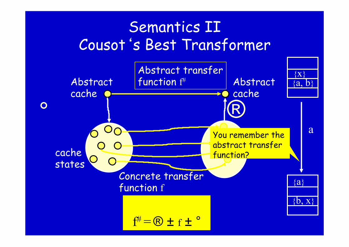
Semantics II Cousot‘s Best Transformer

°

Abstract transfer function f#

Concrete transfer function f

® cache states

Abstract cache

Abstract cache

{a, b} {x}

a

{b, x}

{a}

You remember the abstract transfer function?

f# = ® ± f ± °

Lessons Learned

•  Cache analysis, an important ingredient of static timing analysis, provides for abstract domains,

•  which proved to be sufficiently precise, •  have compact representation, •  have efficient transfer functions, •  which are quite natural.

An Alternative Abstract Cache Semantics: Power set domain of cache states

•  Set A of elements - sets of concrete cache states

•  Information order v - set inclusion •  Join operator t - set union •  Top element > - the set of all cache

states •  Bottom element ? - the empty set of

caches

Problem Solved? •  We have shown a solution for LRU caches. •  LRU-cache analysis works smoothly

–  Favorable „structure“ of domain –  Essential information can be summarized compactly

•  LRU is the best strategy under several aspects –  performance, predictability, sensitivity

•  … and yet: LRU is not the only strategy –  Pseudo-LRU (PowerPC 755 @ Airbus) –  FIFO –  worse under almost all aspects, but average-case

performance!

Structure of the Lectures 1.  Introduction 2.  Static timing analysis


3.  Cache analysis 4.  Pipeline analysis 5.  Value analysis 6.  Worst-case path analysis ----------------------------------------------------------- 1.  Timing Predictability


2.  Conclusion

Tool Architecture



Pipelines

Hardware Features: Pipelines

Ideal Case: 1 Instruction per Cycle

Fetch Decode

Execute

WB

Fetch Decode

Execute

WB

Inst 1 Inst 2 Inst 3 Inst 4

Fetch Decode

Execute WB

Fetch Decode

Execute

WB

Fetch Decode

Execute

WB

Pipelines

•  Instruction execution is split into several stages

•  Several instructions can be executed in parallel •  Some pipelines can begin more than one

instruction per cycle: VLIW, Superscalar •  Some CPUs can execute instructions out-of-

order •  Practical Problems: Hazards and cache misses

Pipeline Hazards

Pipeline Hazards: •  Data Hazards: Operands not yet available

(Data Dependences) •  Resource Hazards: Consecutive

instructions use same resource •  Control Hazards: Conditional branch •  Instruction-Cache Hazards: Instruction

fetch causes cache miss

Cache analysis: prediction of cache hits on instruction or operand fetch or store

Static exclusion of hazards

lwz r4, 20(r1) Hit

Dependence analysis: elimination of data hazards

Resource reservation tables: elimination of resource hazards

add r4, r5,r6 lwz r7, 10(r1) add r8, r4, r4

Operand ready

IF"EX"M"F"

CPU as a (Concrete) State Machine

•  Processor (pipeline, cache, memory, inputs) viewed as a big state machine, performing transitions every clock cycle

•  Starting in an initial state for an instruction transitions are performed, until a final state is reached: –  End state: instruction has left the pipeline – # transitions: execution time of instruction

A Concrete Pipeline Executing a Basic Block

function exec (b : basic block, s : concrete pipeline state) t: trace

interprets instruction stream of b starting in state s producing trace t.

Successor basic block is interpreted starting in initial

state last(t) length(t) gives number of cycles

An Abstract Pipeline Executing a Basic Block

function exec (b : basic block, s : abstract pipeline state) t: trace

interprets instruction stream of b (annotated with cache information) starting in state s producing trace t

length(t) gives number of cycles

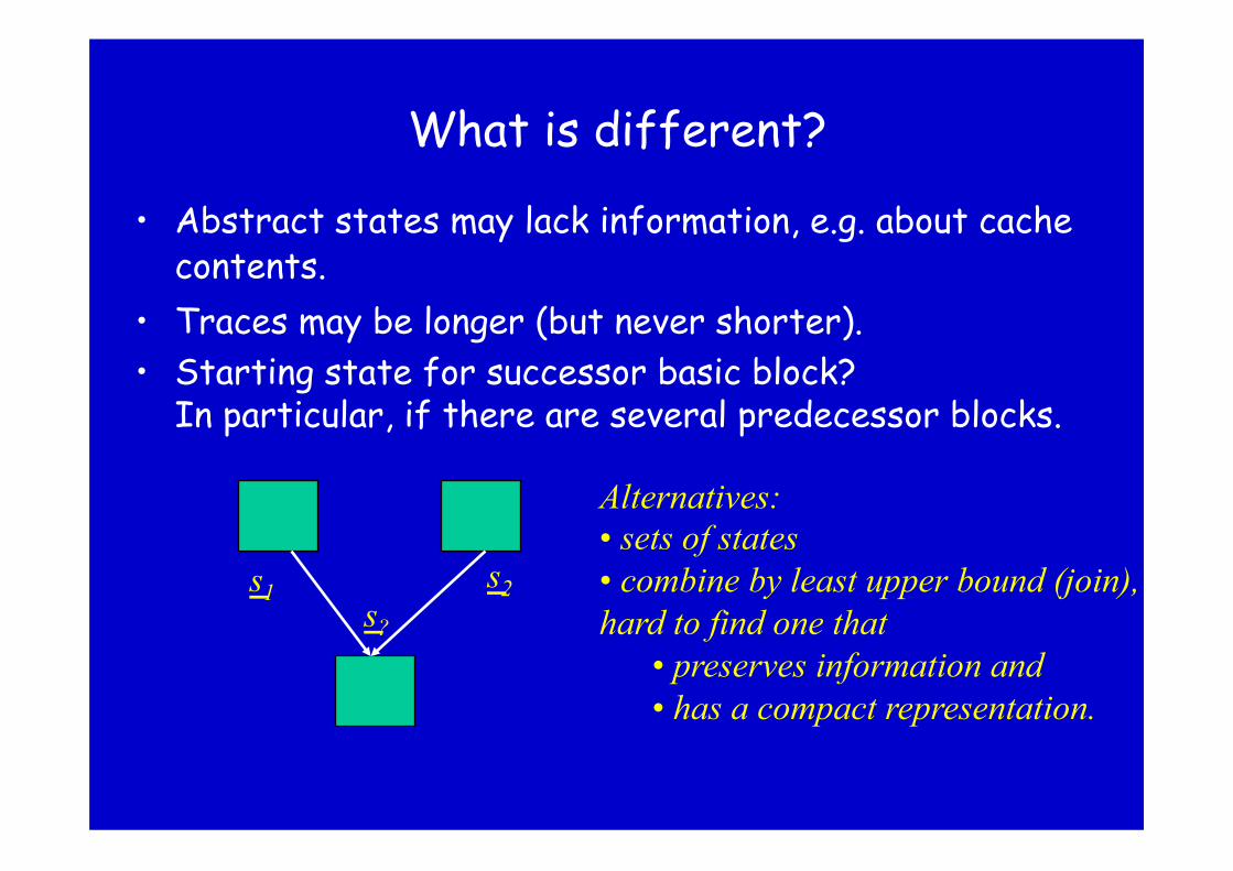
What is different?

•  Abstract states may lack information, e.g. about cache contents.

•  Traces may be longer (but never shorter). •  Starting state for successor basic block?

In particular, if there are several predecessor blocks.

s2 s1 s?

Alternatives: •  sets of states •  combine by least upper bound (join), hard to find one that

•  preserves information and •  has a compact representation.

Non-Locality of Local Contributions •  Interference between processor components

produces Timing Anomalies: –  Assuming local best case leads to higher overall

execution time. –  Assuming local worst case leads to shorter overall

execution time Ex.: Cache miss in the context of branch prediction

•  Treating components in isolation may be unsafe •  Implicit assumptions are not always correct:

–  Cache miss is not always the worst case! –  The empty cache is not always the worst-case

start!

An Abstract Pipeline Executing a Basic Block - processor with timing anomalies -

function analyze (b : basic block, S : analysis state) T: set of trace

Analysis states = 2PS x CS PS = set of abstract pipeline states CS = set of abstract cache states

interprets instruction stream of b (annotated with cache information) starting in state S producing set of traces T

max(length(T)) - upper bound for execution time last(T) - set of initial states for successor block Union for blocks with several predecessors.

S2 S1 S3 =S1 ∪S2

Integrated Analysis: Overall Picture

Basic Block

s1

s10

s2 s3

s11 s12

s1

s13

Fixed point iteration over Basic Blocks (in context) {s1, s2, s3} abstract state

move.1 (A0,D0),D1

Cyclewise evolution of processor model for instruction

s1 s2 s3

Classification of Pipelines •  Fully timing compositional architectures:

–  no timing anomalies. –  analysis can safely follow local worst-case paths only, –  example: ARM7.

•  Compositional architectures with constant-bounded effects: –  exhibit timing anomalies, but no domino effects, –  example: Infineon TriCore

•  Non-compositional architectures: –  exhibit domino effects and timing anomalies. –  timing analysis always has to follow all paths, –  example: PowerPC 755

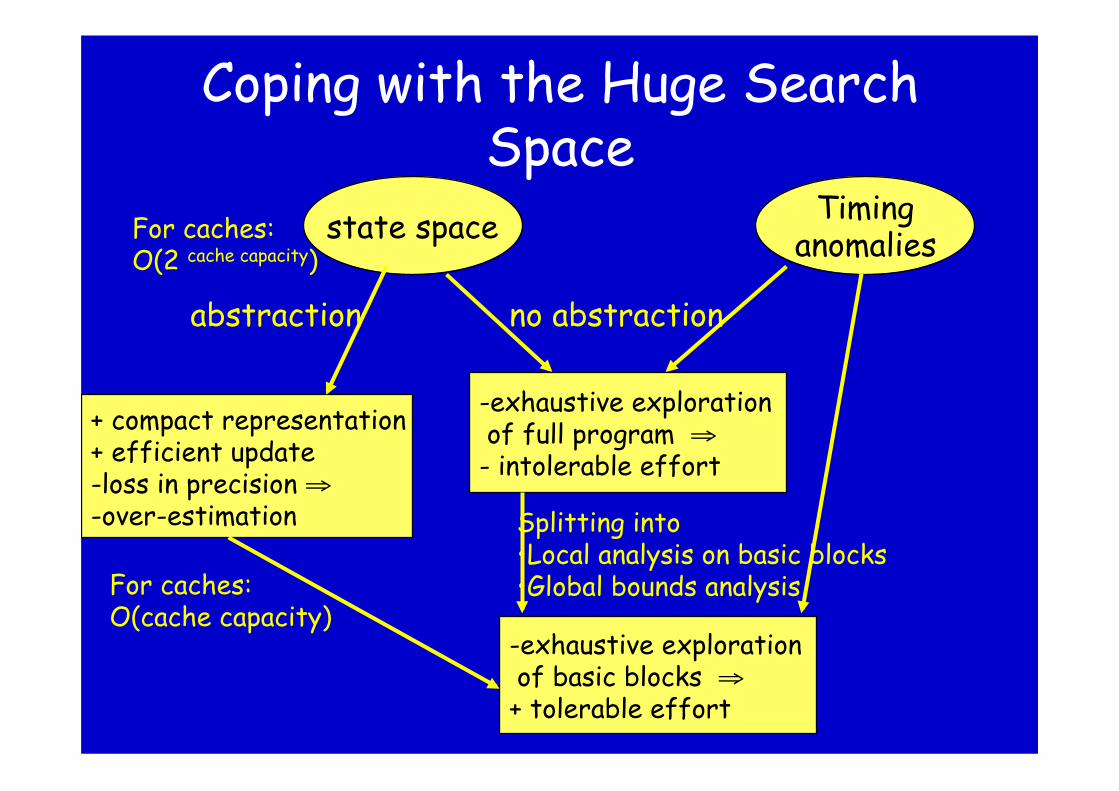
Coping with the Huge Search Space

state space

+ compact representation + efficient update - loss in precision ⇒ - over-estimation

Timing anomalies

abstraction no abstraction

- exhaustive exploration of full program ⇒ -  intolerable effort

- exhaustive exploration of basic blocks ⇒ + tolerable effort

Splitting into • Local analysis on basic blocks • Global bounds analysis

For caches: O(2 cache capacity)

For caches: O(cache capacity)

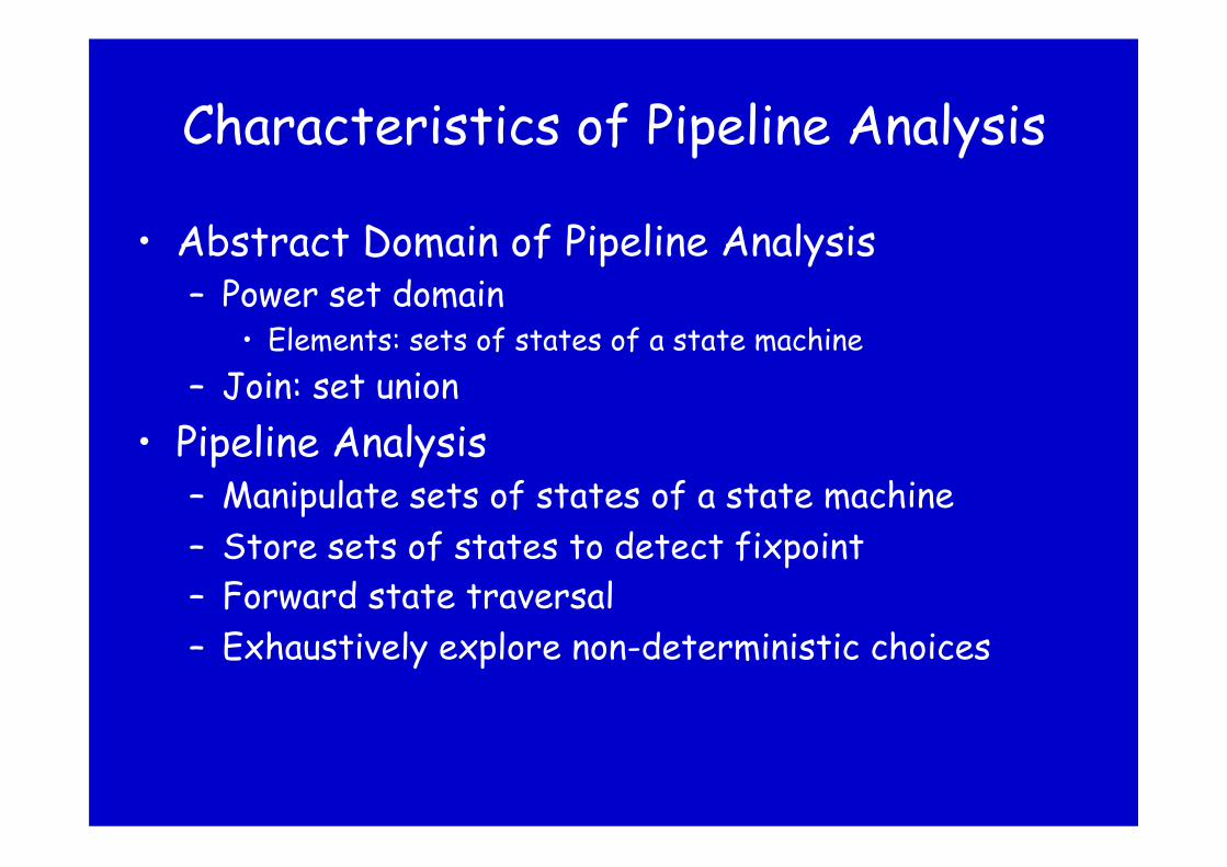
Characteristics of Pipeline Analysis

•  Abstract Domain of Pipeline Analysis –  Power set domain

•  Elements: sets of states of a state machine –  Join: set union

•  Pipeline Analysis –  Manipulate sets of states of a state machine –  Store sets of states to detect fixpoint –  Forward state traversal –  Exhaustively explore non-deterministic choices

Tool Architecture



Value Analysis •  Motivation:

–  Provide access information to data-cache/pipeline analysis

–  Detect infeasible paths –  Derive loop bounds

•  Method: calculate intervals at all program points, i.e. lower and upper bounds for the set of possible values occurring in the machine program (addresses, register contents, local and global variables) (Cousot/Cousot77)

Value Analysis II

•  Intervals are computed along the CFG edges

•  At joins, intervals are „unioned“

D1: [-2,+2] D1: [-4,0]

D1: [-4,+2]

move.l #4,D0

add.l D1,D0

move.l (A0,D0),D1

D1: [-4,4], A[0x1000,0x1000]

D0[4,4], D1: [-4,4], A[0x1000,0x1000]

D0[0,8], D1: [-4,4], A[0x1000,0x1000]

access [0x1000,0x1008] Which address is accessed here?

Interval Domain

(-1,0]

(-1,-1] [-2,2] [0,1)

[1,1)

[-2,0]

[-2,-1]

[-2,1] [-1,1] [0,2]

[-1,0] [0,1] [1,2]

[2,2] [1,1] [0,0] [-1,-1] [-2,-2]

[-1,2]

(-1,1)

[-1,1) (-1,1]

1 he

ight

Interval Analysis in Timing Analysis

•  Data-cache analysis needs effective addresses at analysis time to know where accesses go.

•  Effective addresses are approximatively precomputed by an interval analysis for the values in registers, local variables

•  “Exact” intervals – singleton intervals, •  “Good” intervals – addresses fit into less

than 16 cache lines.

Value Analysis (Airbus Benchmark) Task Unreached Exact Good Unknown Time [s]

1 8% 86% 4% 2% 47 2 8% 86% 4% 2% 17 3 7% 86% 4% 3% 22 4 13% 79% 5% 3% 16 5 6% 88% 4% 2% 36 6 9% 84% 5% 2% 16 7 9% 84% 5% 2% 26 8 10% 83% 4% 3% 14 9 6% 89% 3% 2% 34

10 10% 84% 4% 2% 17 11 7% 85% 5% 3% 22 12 10% 82% 5% 3% 14

1Ghz Athlon, Memory usage <= 20MB

Tool Architecture



•  Execution time of a program = ∑ Execution_Time(b) x

Execution_Count(b)

•  ILP solver maximizes this function to determine the WCET

•  Program structure described by linear constraints –  automatically created from CFG structure –  user provided loop/recursion bounds –  arbitrary additional linear constraints to

exclude infeasible paths

Basic_Block b

Path Analysis by Integer Linear Programming (ILP)

if a then b elseif c then d else e endif f

a

b c

d

f

e

10t

4t

3t

2t

5t

6t

max: 4 xa + 10 xb + 3 xc + 2 xd + 6 xe + 5 xf where xa = xb + xc

xc = xd + xe xf = xb + xd + xe xa = 1

Value of objective function: 19 xa 1 xb 1 xc 0 xd 0 xe 0 xf 1

Example (simplified constraints)



3.  Cache analysis 4.  Pipeline analysis 5.  Value analysis ----------------------------------------------------------- 1.  Timing Predictability


2.  Conclusion

Timing Predictability Experience has shown that the precision of results

depend on system characteristics •  of the underlying hardware platform and •  of the software layers •  We will concentrate on the influence of the HW

architecture on the predictability What do we intuitively understand as

Predictability? Is it compatible with the goal of optimizing

average-case performance? What is a strategy to identify good compromises?





2.  Conclusion

Predictability of Cache Replacement Policies

Uncertainty in Cache Analysis

read y

mul x, y

read x

write z

1. Initial cache contents?2. Need to combine information3. Cannot resolve address of x...4. Imprecise analysis domain/ update functions

Need to recover information: Predictability = Speed of Recovery

Metrics of Predictability: ...

......

[f,e,d]

[f,e,c]

[f,d,c]

[h,g,f]

fillevict

Seq: a b c d e f g h

Two Variants: M = Misses Only HM

evict & fill

Meaning of evict/fill - I

•  Evict: may-information: – What is definitely not in the cache? –  Safe information about Cache Misses

•  Fill: must-information: – What is definitely in the cache? –  Safe information about Cache Hits

Meaning of evict/fill - II

Metrics are independent of analyses:

à  evict/fill bound the precision of any static analysis!

à  Allows to analyze an analysis: Is it as precise as it gets w.r.t. the metrics?

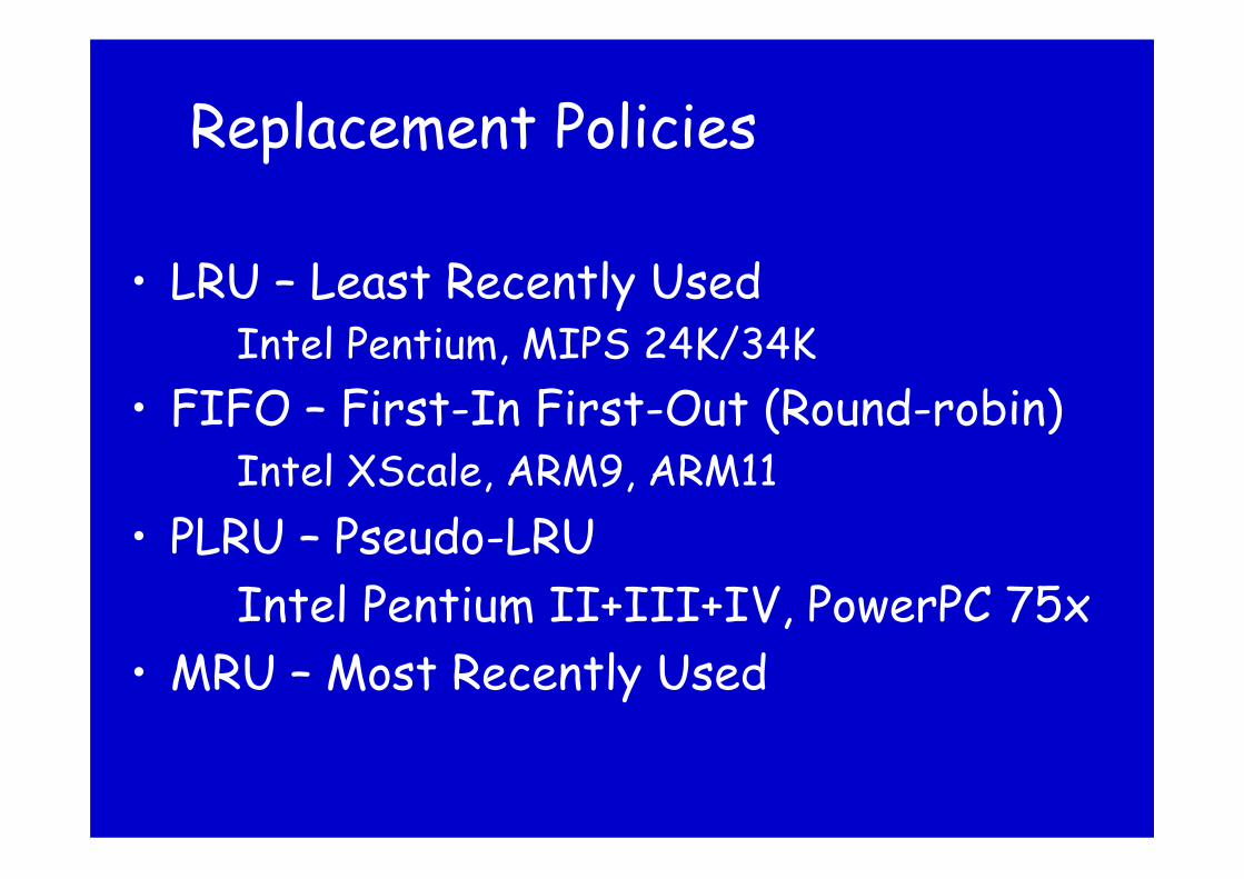
Replacement Policies

•  LRU – Least Recently Used Intel Pentium, MIPS 24K/34K

•  FIFO – First-In First-Out (Round-robin) Intel XScale, ARM9, ARM11

•  PLRU – Pseudo-LRU Intel Pentium II+III+IV, PowerPC 75x

•  MRU – Most Recently Used

MRU - Most Recently Used

MRU-bit records whether line was recently used

Problem: never stabilizes

e

cb,d

c „safe“for 5 acc.

Tree maintains order: Problem: accesses „rejuvenate“

neighborhood

Pseudo-LRU

cà

eà

Results: tight bounds

Results: tight bounds

Generic examples prove tightness.

Results: instances for k=4,8

Question: 8-way PLRU cache, 4 instructions per line Assume equal distribution of instructions over

256 sets: How long a straight-line code sequence is needed to

obtain precise may-information?

Future Work I

•  OPT = theoretical strategy,

optimal for performance •  LRU = used in practice,

optimal for predictability •  Predictability of OPT? •  Other optimal policies for predictability?

OPT for performanceLRU for predictability=

?

Future Work II

Beyond evict/fill: •  Evict/fill assume complete uncertainty

•  What if there is only partial

uncertainty? •  Other useful metrics?

LRU has Optimal Predictability, so why is it Seldom Used?

•  LRU is more expensive than PLRU, Random, etc. •  But it can be made fast

–  Single-cycle operation is feasible [Ackland JSSC00] –  Pipelined update can be designed with no stalls

•  Gets worse with high-associativity caches –  Feasibility demonstrated up to 16-ways

•  There is room for finding lower-cost highly-predictable schemes with good performance

LRU algorithm

LRU stack MRU LRU

12 3 45 607

Hit in 0 MRU LRU

1 3 4 602 5 7

•  Trivial, but requires an associative search-and-shift operation to locate and promote a bank to the top of the stack.

•  It would be too time consuming to read the stack from the RAM, locate and shift the bank ID within the stack, and write it back to the RAM in a single cycle.

LRU HW implementation [Ackland JSSC00] LRU info is available in one cycle

•  LRU-RAM produces LRU states for lines @ current ADDR •  Stores updates when state is written back: LRU is available

at the same cycle when a MISS is detected

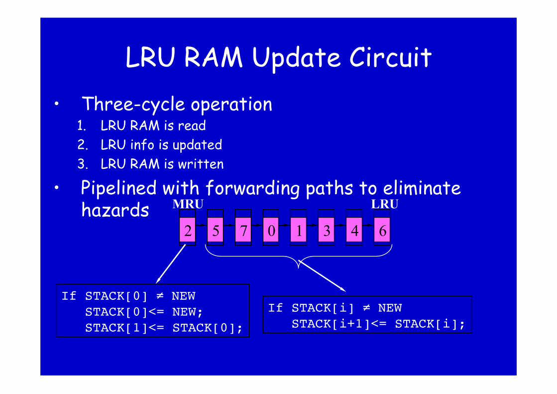
LRU RAM Update Circuit •  Three-cycle operation

1.  LRU RAM is read 2.  LRU info is updated 3.  LRU RAM is written

•  Pipelined with forwarding paths to eliminate hazards MRU LRU

12 3 45 607

If STACK[0] ≠ NEW "STACK[0]<= NEW;"STACK[1]<= STACK[0];"

If STACK[i] ≠ NEW"STACK[i+1]<= STACK[i];"

Beyond evict/fill

Evolution of may- /must-information (PLRU):

may/must-set sizes

distinct access

sequence

evict(k) fill(k)

log k +1

k





2.  Conclusion

Extended the Predictability Notion

•  The cache-predictability concept applies to all cache-like architecture components:

•  TLBs, BTBs, other history mechanisms

The Predictability Notion Unpredictability •  is an inherent system property •  limits the obtainable precision of static predictions about

dynamic system behavior Digital hardware behaves deterministically (ignoring

defects, thermal effects etc.) •  Transition is fully determined by current state and input •  We model hardware as a (hierarchically structured,

sequentially and concurrently composed) finite state machine

•  Software and inputs induce possible (hardware) component inputs

Uncertainties About State and Input

•  If initial system state and input were known, only one execution (time) were possible.

•  To be safe, static analysis must take into account all possible initial states and inputs.

•  Uncertainty about state implies a set of starting states and different transition paths in the architecture.

•  Uncertainty about program input implies possibly different program control flow.

•  Overall result: possibly different execution times Ed wants to forbid this!

Source and Manifestation of Unpredictability

•  “Outer view” of the problem: Unpredictability manifests itself in the variance of execution time

•  Shortest and longest paths through the automaton are the BCET and WCET

•  “Inner view” of the problem: Where does the variance come from?

•  For this, one has to look into the structure of the finite automata

Variability of Execution Times

•  is at the heart of timing unpredictability, •  is introduced at all levels of granularity

– Memory reference –  Instruction execution –  Arithmetic –  Communication

•  results, in some way or other, from the interference on shared resources.

Connection Between Automata and Uncertainty

•  Uncertainty about state and input are qualitatively different:

•  State uncertainty shows up at the “beginning” ≅ number of possible initial starting states the automaton may be in.

•  States of automaton with high in-degree lose this initial uncertainty.

•  Input uncertainty shows up while “running the automaton”.

•  Nodes of automaton with high out-degree introduce uncertainty.

State Predictability – the Outer View

Let T(i;s) be the execution time with component input i starting in hardware component state s.

The range is in [0::1], 1 means perfectly timing-predictable

The smaller the set of states, the smaller the variance and the larger the predictability.

The smaller the set of component inputs to consider, the larger the predictability.

Input Predictability

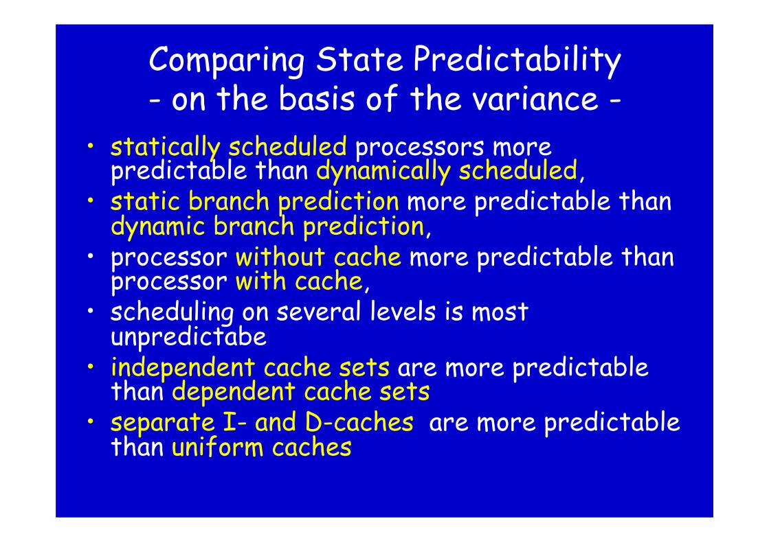
Comparing State Predictability - on the basis of the variance -

•  statically scheduled processors more predictable than dynamically scheduled,

•  static branch prediction more predictable than dynamic branch prediction,

•  processor without cache more predictable than processor with cache,

•  scheduling on several levels is most unpredictabe

•  independent cache sets are more predictable than dependent cache sets

•  separate I- and D-caches are more predictable than uniform caches

Predictability – the Inner View

•  We can look into the automata: •  Speed of convergence •  #reachable states •  #transitions/outdegree/indegree

Processor Features of the MPC 7448

•  Single e600 core, 600MHz-1,7GHz core clock

•  32 KB L1 data and instruction caches

•  1 MB unified L2 cache with ECC •  Up to 12 instructions in

instruction queue •  Up to 16 instructions in parallel

execution •  7 stage pipeline •  3 issue queues, GPR, FPR,

AltiVec •  11 independent execution units

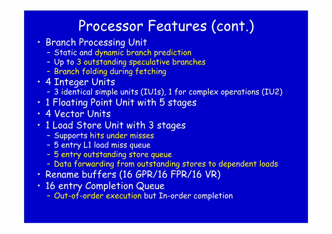
Processor Features (cont.) •  Branch Processing Unit

–  Static and dynamic branch prediction –  Up to 3 outstanding speculative branches –  Branch folding during fetching

•  4 Integer Units –  3 identical simple units (IU1s), 1 for complex operations (IU2)

•  1 Floating Point Unit with 5 stages •  4 Vector Units •  1 Load Store Unit with 3 stages

–  Supports hits under misses –  5 entry L1 load miss queue –  5 entry outstanding store queue –  Data forwarding from outstanding stores to dependent loads

•  Rename buffers (16 GPR/16 FPR/16 VR) •  16 entry Completion Queue

–  Out-of-order execution but In-order completion

Challenges and Predictability •  Speculative Execution

– Up to 3 level of speculation due to unknown branch prediction

•  Cache Prediction – Different pipeline paths for L1 cache hits/misses – Hits under misses –  PLRU cache replacement policy for L1 caches

•  Arbitration between different functional units –  Instructions have different execution times on IU1

and IU2 •  Connection to the Memory Subsystem

– Up to 8 parallel accesses on MPX bus •  Several clock domains

–  L2 cache controller clocked with half core clock – Memory subsystem clocked with 100 – 200 MHz

Architectural Complexity implies

Analysis Complexity Every hardware component whose state has an

influence on the timing behavior •  must be conservatively modeled, •  contributes a multiplicative factor to the size

of the search space.

History/future devices: all devices concerned with storing the past or predicting the future.

Classification of Pipelines •  Fully timing compositional architectures:

–  no timing anomalies. –  analysis can safely follow local worst-case paths only, –  example: ARM7.

•  Compositional architectures with constant-bounded effects: –  exhibit timing anomalies, but no domino effects, –  example: Infineon TriCore

•  Non-compositional architectures: –  exhibit domino effects and timing anomalies. –  timing analysis always has to follow all paths, –  example: PowerPC 755

Recommendation for Pipelines

•  Use compositional pipelines; often execution time is dominated by memory-access times, anyway.

•  Static branch prediction only; •  One level of speculation only

More Threats created by Computer Architects

•  Out-of-order execution

•  Speculation •  Timing Anomalies,

i.e., locally worst-case path does not lead to the globally worst-case path, e.g., a cache miss can contribute to a globally shorter execution if it prevents a mis-prediction.

Consider all possible execution orders

ditto

Considering the locally worst-case path insufficent

First Principles

•  Reduce interference on shared resources. •  Use homogeneity in the design of

history/future devices.

Interference on Shared Resources

•  can be real –  e.g., tasks interfering on buses,

memory, caches •  can be virtual, introduced by

abstraction, e.g., –  unknown state of branch predictor

forces analysis of both transitions ⇒ interference on instruction cache

–  are responsible for timing anomalies

real non-determinism

artificial non-determinism

Design Goal: Reduce Interference on Shared

Resources •  Integrated Modular Avionics (IMA) goes

in the right direction – temporal and spatial partitioning for eliminating logical interference

•  For predictability: extension towards the elimination/reduction of physical interference

Shared Resources between Threads on Different Cores

•  Strong synchronization ⇒ low performance

•  Little synchronization ⇒ many potential interleavings ⇒ high complexity of analysis

Recommendations for Architecture Design

Architecture follows application: Exploit information about the application in the architecture design.

Design architectures to which applications can be mapped without introducing extra interferences.

Form follows function, (Louis Sullivan)

Recommendation for Application Designers

•  Use knowledge about the architecture to produce an interference-free mapping.

Separated Memories

•  Characteristic of many embedded applications: little code shared between several tasks of an application ⇒ separate memories for code of threads running on different cores

Shared Data •  Often:

–  reading data when task is started, –  writing data when task terminate

•  deterministic scheme for access to shared data memory required cache performance determines –  partition of L2-caches –  bus schedule

•  Crossbar instead of shared bus

Conclusion

•  Feasibility, efficiency, and precision of timing analysis strongly depend on the execution platform.

•  Several principles were proposed to support timing analysis.

Current Research

•  Extension of timing analysis to multi-core platforms –  threads on different cores interfere on shared

resources –  reduce performance compared to single-core

performance –  introduce uncertainty about when accesses will

happen •  Design for predictability

Lecture Course in Winter 2012/2013

•  Embedded System Design •  RW with Daniel Kästner and Florian

Martin (AbsInt) •  Practical aspects of embedded-systesm

design – methods –  tools –  projects

Some Relevant Publications from my Group •  C. Ferdinand et al.: Cache Behavior Prediction by Abstract Interpretation. Science of

Computer Programming 35(2): 163-189 (1999) •  C. Ferdinand et al.: Reliable and Precise WCET Determination of a Real-Life Processor,

EMSOFT 2001 •  R. Heckmann et al.: The Influence of Processor Architecture on the Design and the

Results of WCET Tools, IEEE Proc. on Real-Time Systems, July 2003 •  St. Thesing et al.: An Abstract Interpretation-based Timing Validation of Hard Real-Time

Avionics Software, IPDS 2003 •  L. Thiele, R. Wilhelm: Design for Timing Predictability, Real-Time Systems, Dec. 2004 •  R. Wilhelm: Determination of Execution Time Bounds, Embedded Systems Handbook, CRC

Press, 2005 •  St. Thesing: Modeling a System Controller for Timing Analysis, EMSOFT 2006 •  J. Reineke et al.: Predictability of Cache Replacement Policies, Real-Time Systems,

Springer, 2007 •  R. Wilhelm et al.:The Determination of Worst-Case Execution Times - Overview of the

Methods and Survey of Tools. ACM Transactions on Embedded Computing Systems (TECS) 7(3), 2008.

•  R.Wilhelm et al.: Memory Hierarchies, Pipelines, and Buses for Future Architectures in Time-critical Embedded Systems, IEEE TCAD, July 2009

•  D. Grund, J. Reineke: Precise and Efficient FIFO-Replacement Analysis Based on Static Phase Detection. ECRTS 2010

•  Daniel Grund, Jan Reineke: Toward Precise PLRU Cache Analysis. WCET 2010 •  S.Altmeyer, C. Maiza, J. Reineke: Resilience analysis: tightening the CRPD bound for set-

associative caches. LCTES 2010 •  S. Altmeyer, C. Maiza: Cache-related preemption delay via useful cache blocks: Survey and

redefinition. Journal of Systems Architecture - Embedded Systems Design 57(7), 2011

Documents

Timing Analysis - uni-saarland.de · Structure of the Lecture 1. Introduction 2. Static timing analysis 1. the problem 2. our approach 3. the success 4. tool architecture