Timing analysis of compound scheduling policies: application to

Posix1003.1b

Jorn Migge2, Alain Jean-Marie1, Nicolas Navet2

1 LIRMM 2 LORIA - CNRS UMR 7503Departement IFA TRIO Team - ENSEM

161 Rue Ada 2, Avenue de la foret de HayeF-34392 Montpellier Cedex 05 F-54516 Vandoeuvre-les-Nancy

January 24, 2002

Abstract

The analysis of fixed priority preemptive scheduling has been extended in variousways to improve its usefulness for the design of real-time systems. In this paper,we define the layered preemptive priority scheduling policy which generalizes fixedpreemptive priorities by combination with other policies in a layered structure. Inparticular, the combination with the Round Robin scheduling policy is studied. Itscompliance with Posix 1003.1b requirements is shown and its timing analysis isprovided. For this purpose and as a basis for the analysis of other policies, theconcept of majorizing work arrival function, is introduced to synthesize essentialideas used in existing analysis of the fixed preemptive priority policy.If critical resources are protected by semaphores, the Priority Ceiling Protocol (PCP)can be used under fixed preemptive priorities to control resulting priority inversions.An extension of the PCP is proposed for Round Robin, to allow a global control ofpriority inversions under the layered priority policy and to prevent deadlocks. Theinitial timing analysis is extended to account for the effects of the protocol. Theresults are illustrated by a small test case.

1

1 Introduction

A real-time system is typically composed of a controlling system and a controlled system.The timing constraints on the controlling system’s activities arise from the dynamics of thecontrolled system. For the satisfaction of these constraints a correct schedule of the system’sactivities needs to be found.

In this paper we introduce the layered preemptive priority scheduling policy, LPP for short.It allows to combine different policies in a layered structure, based on the fixed preemptivepriority scheduling policy, FPP for short. The techniques used in the timing analysis of FPPhave evolved with the attempts at accounting more precisely for the characteristics of real-world systems. In this paper we propose a framework that synthesizes the essential ideas ofthese techniques. We apply the framework to the analysis of the LPP policy, of which theFPP policy is a special case.

The FPP policy was initially analyzed by Liu & Layland [1] for periodic tasks with dead-lines equal to their period. It has been shown that the maximal response time of a task occursafter the critical instant, defined as a time where all tasks are released simultaneously. Onlythis response time needs to be analyzed to decide upon feasibility. A task set is said to befeasible if each task always meets its deadlines at run-time. A sufficient feasibility test hasbeen derived from this property, based on a bound of the tasks’s average processor utilization.A necessary and sufficient feasibility test has been derived by Lehoczky et al. [2], based on atest-function, that must be evaluated at certain times between the release and the deadlineof a task. A different approach was introduced by Joseph & Pandya in [3]. Their idea isto compute the response time of a task after the critical instant and to compare it with thedeadline. The actual computations however are quite similar in both cases.

In order to apply the test-function based approach in the case where deadlines are setbeyond the task periods, Lehoczky introduced in [4] the concept of busy period, which wasthen also used for the analysis based on response time computation in [5] by Tindel et al.Basically, the busy period that starts with the critical instant has to be analyzed to determinethe worst case response time. More generally, the critical instant can be seen as the beginningof a worst case release pattern.

In this paper we formalize these worst case release patterns by introducing the concept of(majorizing) work arrival function. The purpose is to provide a timing analysis frameworkthat allows to easily integrate new types of tasks and policies with results already known.Work arrival functions (WAF, for short) allow in particular to write response time formulasand response time bounds for a given policy independently of a specific type of task usedas model for a real-world task. As a result, timing analysis can be split into two parts, oneconcerned with the analysis of worst-case behaviors of tasks in terms of majorizing workarrival functions (MWAF, for short) and a second which uses MWAF and is only concernedwith analysis of the specific properties of the scheduling policy. The analysis of a new policycan then rely on known MWAF, and the MWAF of a new task model can be integrated intothe analysis of a known policy. This approach is especially useful in the analysis of morecomplex policies such as the layered preemptive priority scheduling policy, that we introducein this paper. This scheduling policy uses the layered structure of fixed priorities to combinedifferent policies. We shall restrict our study to the combination of FPP and the RoundRobin policy (RR, for short), motivated by the Posix 1003.1b standard. According to thisstandard, (real-time) operating systems have to provide at least these two scheduling policiesfor a side-by-side use. With Round Robin, the question of efficiently handling semaphores has

2

to be reconsidered. Under preemptive policies, semaphores are used to prevent preemptionduring the use of critical resources. This leads to longer response times for higher prioritytasks, because of priority inversions. To limit this effect and to avoid possible deadlockswith nested access to resources, the priority ceiling protocol has been proposed by Sha et al.in [6] for FPP. Applied ”as is” to Round Robin, the Priority Ceiling Protocol (PCP) doesnot prevent deadlocks. Furthermore, semaphores distort the processor access rates which areusually guaranteed by the Round Robin scheduling policy. This is similar to the priorityinversions under FPP. In this paper we define a first extension of the PCP that prevents fromdeadlocks and a second that controls the access rates. The first extension can be implementedunder Posix. The second requires some modifications, but allows a more accurate timinganalysis.

The paper is organized as follows. In Section 2, the Posix 1003.1b standard is brieflydescribed and in Section 3 the layered preemptive priority policy is defined and its linkwith the Posix 1003.1b standard is explained. In Section 4 the concept of majorizing workarrival function is introduced to derive general response time bounds under FPP and alsoRR, in Section 5. The definition of the priority ceiling protocol for Round Robin and thecorresponding timing analysis are given in Section 6. A numerical example is proposed inSection 7 and a conclusion is given in Section 8.

2 Posix 1003.1b scheduling

Posix 1003.1b standard [7], formerly Posix.4, defines real-time extensions to Posix.1 mainlyconcerning signals, inter-process communication, memory mapped files, memory locking, syn-chronized and asynchronous I/O, timers and scheduling policies. Most of today’s real-timeoperating systems conform, at least partially, to this standard.Posix 1003.1b specifies three scheduling policies : SCHED RR, SCHED FIFO and SCHED-OTHER. These policies apply on a process-by-process basis : each process runs with a par-ticular policy and a given priority. Each process inherits its scheduling parameters from itsfather but may also change them at run-time.

• SCHED FIFO : fixed preemptive priority with FIFO ordering among same priorityprocesses.

• SCHED RR : round-robin policy which allows processes of same priority to share theprocessing unit. Note that a process will not get the CPU until all higher priority ready-to-run processes are executed. The quantum value may be a system-wide constant,process specific or fixed for a given priority level.

• SCHED OTHER is an implementation-defined scheduler. It could map onto SCHED RRor SCHED FIFO or also implement a classical Unix time-sharing policy. The standardmerely mandates its presence and its documentation. Because it is not possible to expectthe same behavior of SCHED OTHER under all Posix compliant operating systems, itis strongly suggested not to use it if portability is a matter of concern and we will notconsider it in our analysis.

Associated with each policy is a priority range. Depending on the implementation, thesepriority ranges may or may not overlap. In the case where priority ranges overlap, taskswith policy flags SCHED FIFO or SCHED RR may have the same priority. Our analysis can

3

handle this case if these SCHED FIFO flags are changed to SCHED RR and the quantum isset to the tasks worst case execution time (WCET).

Note that these scheduling mechanisms similarly apply to Posix threads standardized byPosix 1003.1c standard. Threads, defined in [7] as single flows of control within a process, area means of providing multiple “lightweight” processes within one process address space. Theproblem with threads is that some aspects of their scheduling are not covered by the standard.The concept of the scheduling contention scope of a thread defines the set of threads withwhich it has to compete for the use of processing resources :

• A thread created with the system contention scope, regardless of the process in whichit resides, competes with all processes and all other threads which have the systemscheduling contention scope. The analysis that is further developed equally applies tosystem-wide contention threads.

• A thread created with the process contention scope only competes with other threadswithin its process having the process scheduling contention scope. In the standard,it is unspecified how such “process contention scope” threads are scheduled relativeto threads belonging to other processes and relative to other processes. Because theprocess contention scope scheduling is OS-dependent, we will not further consider itsuse.

In the rest of the paper, we define a task as a recurrent activity. A task may be implementedeither by a process (resp. thread) which is repetitively launched or by a unique process (resp.thread) that runs in cycles.

3 Layered Priorities

We now define the layered preemptive priority scheduling policy for a set of recurrent tasksT = {τ1, . . . , τm}. A task is recurrent if at any time there is a next release of the task that willoccur in the future. The simplest example are periodic tasks. Since for each release the taskmay have a different execution time and the time since the previous release may be differenttoo, we wish to be able to consider each release individually. Therefore, we call a release aninstance of the task; the nth instance of τk is denoted τk,n.

The policy is defined in two steps. The first step specifies the layer structure and thesecond the internal structure of the layers.

Let the set of tasks be partitioned into layers λl = {τk |ml−1 < k 6 ml} , where l = 1, 2, . . .and 1 6 ml−1 < ml 6 m, with m0 = 0, see Table 1. Suppose they are scheduled according tothe global rule: an instance τk,n of a task τk in a layer λl is executed as soon as and as longas no instance in the (higher priority) layers λ1, . . . , λl−1 is pending.

So far the scheduling rule is incomplete since it does not tell how tasks are scheduled insideof a layer. The fixed preemptive priority scheduling policy (FPP) can be realized inside ofa layer λl by applying the same rule again, i.e. an instance of τk ∈ λl is executed as soonas and as long as no instance of a (higher priority) task τj , ml−1 < j < k in the same layerλl is pending. Under POSIX this can be implemented by giving to each task of the layer adifferent priority with the SCHED FIFO attribute in a reserved subrange of priorities. TheRound Robin scheduling policy can be realized inside of a layer by assigning the same priorityto all tasks of the layer with the SCHED RR attribute and some time quantum to each task

4

Layer ml Tasks Policy-Flag Priority Quantumλ1 (FPP) τ1 SCHED FIFO 1 -

τ2 SCHED FIFO 2 -τ3 SCHED FIFO 3 -

m1 = 4 τ4 SCHED FIFO 4 -λ2 (RR) τ5 SCHED RR 5 15

τ6 SCHED RR 5 5m2 = 7 τ7 SCHED RR 5 10

λ3 (FPP) τ8 SCHED FIFO 6 -τ9 SCHED FIFO 7 -τ10 SCHED FIFO 8 -τ11 SCHED FIFO 9 -

m3 = 12 τ12 SCHED FIFO 10 -

Table 1: Example of Layered Priorities (under Posix 1003.1b)

that tells how long it is allowed to execute without being interrupted by the RR-scheduler.The priority must of course be reserved for tasks of the RR-layer.

Notice that the policy in a layer could be any non-idling policy such as earliest deadlinefirst, last in first out, etc. Following this idea it is possible to define LPP in a more generalmanner in terms of priority functions. The interested reader is referred to [8].

4 Fixed preemptive priorities

To be able to analyze a layered preemptive priority policy based on FPP and RR, we have toreformulate the existing FPP timing analysis in this section. Computation of response timebounds are always based on task models. At the beginning a simple model based on worst-caseinter-release and execution times [3], [5] has been used. Some tasks however do not achievethe corresponding peak-rate for an arbitrarily long period of time and thus their worst-casedemand is overestimated. The resulting response time bounds are rather pessimistic. Withthat kind of approach the worst-case behavior of a task is actually associated with that of aperiodic task, even if its worst-case behavior is different. To improve the analysis, other taskmodels have been defined, such as sporadically periodic tasks [5] and multi-frame tasks [9](see Section 4.2. Response time bounds have been derived in [5] and a feasibility test in [9].In this section, we present these known results in a general manner to give a synthetic viewof the common underlying ideas and to extend the analysis to layered priorities. At the end,we provide a generic algorithm for computing response times, based on the general conceptof majorizing work arrival function.

4.1 Interference periods and Response Times

In this section we present a response time formula for an instance of a task scheduled underFPP. The formula is based on work arrival functions and interference periods. It does notinvolve deadlines, and is therefore valid whatever their values are. For a detailed discussionthe reader is referred to [8].

5

For the purpose of deriving a response time formula for an instance τk,n of a task τkwe have to introduce some notations. Let Ck,n ∈ R+ and Ak,n ∈ R+ be the execution andrelease time of the nth instance of τk on a trajectory of the system. By definition, beyondits activation or release time, an instance is ready for execution, meaning that further delaysare only due to the scheduler and no other reasons. The time between two releases is calledcycle time and is denoted Tk,n with the convention Ak,n+1 = Ak,n + Tk,n. Notice that thecycle times of a task are not necessarily equal to a period, but may be different for eachinstance. We make however the assumption that Tk,n > 0, so that consecutive instances arenever released simultaneously. The execution end of τk,n is denoted Ek,n and its responsetime is Rk,n = Ek,n −Ak,n.

The execution end depends on several factors. First of all, the instance τk,n may start toexecute only after the previous instances of τk have completed. Furthermore, while τk,n is exe-cuted it is preempted to satisfy incoming demands from the higher priority tasks τ1, . . . , τk−1.Notice that whether the tasks in higher priority layers are scheduled under Round Robin orFPP, all their demands must be satisfied first. This represents a total amount of work to beexecuted between Ak,n and Ek,n, which can be subdivided into two parts.

One part consists in the remaining work of higher priority instances released strictly beforeAk,n and still pending at Ak,n. Let the remaining work of a task τi at some time t be denotedby Wi(t). With W1..i(t) =

∑ij=1Wj(t), the pending higher priority work is W1..k(Ak,n).

The second part is due to the releases of higher priority tasks during [Ak,n, Ek,n). For thiskind of work we introduce work arrival functions, WAF for short. For a task τk, it is definedfor every interval [a, b) by

Sk(a, b) =∑j∈N

Ck,j · 1I[a6Ak,j<b]. (1)

The indicator function 1I[.] takes the value 1 if the release time Ak,j is situated in [a, b),otherwise 0. Thus the WAF returns the sum of the execution times of all the task released in[a, b). Its value is the sum of all demands from instances of τk released in the given interval[a, b). Notice that WAF’s are additive on adjacent intervals:

Sk(a, b) + Sk(b, c) = Sk(a, c). (2)

With S1..i(a, b) =∑i

k=1 Sk(a, b), the execution end of τk,n can now be written as

Ek,n = min{t > Ak,n |W1..k(Ak,n) + Ck,n + S1..k−1(Ak,n, t) = t−Ak,n}.

It is the first time afterAk,n where the sum of initially pending higher priority workW1..k(Ak,n),the execution time Ck,n of the instance and the arriving higher priority work S1..k−1(Ak,n, t)is equal to the available processing time t−Ak,n. Notice that we have defined WAF’s so thatS1..k−1(Ak,n, t) does not account for releases that may occur at t, because a higher priorityinstance arriving “at the end” of the interval [Ak,n, t) inside of which τk,n is able to completecan not preempt τk,n.

To be able to derive response time bounds from the execution end formula it is usefulto express the pending work W1..k(Ak,n) in terms of WAF. There is a time Uk before Ak,n,where pending work of the tasks τ1, . . . , τk is zero:

Definition 1A level-k interference period is a time interval [Uk, V k) such that already activated instances

of tasks with a priority higher or equal to k are pending neither at its beginning Uk nor at itsend V k, but at any other time between Uk and V k there is at least one such instance pending.

6

The tasks “with a priority higher than k” are all those from higher priority layers, i.e.τ1, . . . , τml−1

, plus the higher priority tasks in the same layer, i.e. τml−1+1, . . . , τk−1.By “already activated” we mean that the activation time must be strictly before the

considered time. Therefore, at any time t ∈ [Uk, V k), there is at least one pending instance,i.e. the demands are higher than the available processing time, and thus

V k = min{t > Uk | S1..k(Uk, t) = t− Uk}. (3)

We denote by Uk,n = Uk the beginning and by Vk,n the end of the level-k interference periodin which τk,n is released, i.e. that contains Ak,n. Notice the following property:

Ak,i ∈ [Uk,n, Vk,n), for n > k + 1 ⇒ Ak,i < Ek,i−1, (4)

which means that inside a level-k interference period, all instances of τk, except the first one,are activated strictly before the previous instances has completed. The strict inequality isimplied by the fact that the definition requests that “already activated instances of taskswith a priority higher or equal to k are pending”. At a point where Ak,i = Ek,i−1, there isno ”already activated instances of tasks with a priority higher or equal to k are pending”since τk,i−1 is completing and because τk,i is activated just at that time - and not before. Theterm ”interference” is precisely motivated by this fact: inside an interference period, at eachmoment, pending work from the past has an influence on present or future executions andthe corresponding response times; this is not the case at a time where Ak,i = Ek,i−1, becauseτk,i is activated when no work from the past is pending, see also the remark below.

The pending higher priority work W1..k(Ak,n) is the result of the arrivals since Uk,n andthe available processing time Ak,n−Uk,n. More precisely, since during the interval [Uk,n, Ak,n)only instances of the tasks τ1, . . . , τk are able to execute,

W1..k(Ak,n) = S1..k(Uk,n, Ak,n)− (Ak,n − Uk,n).

For the execution time of previous instances of τk and the considered instance τk,n itselfwe introduce

Snk = Sk(Uk,n, Ak,n) + Ck,n. (5)

Thus the execution end Ek,n of τk,n satisfies

Ek,n = min{t > Uk,n | S1..k−1(Uk,n, t) + Snk = t− Uk,n}. (6)

The execution end is the smallest solution of a fixed point equation, see Appendix A. If theterm S1..k−1(Uk,n, t) is replaced by a function that majorizes the term for every time t, thenthe solution of the new fixed point equation is larger than Ek,n, i.e. it is a bound for Ek,n.This fact, and the the concept of majorizing work arrival function introduced in the nextsection will allows us to derive response time bounds.Remark: In [4], Lehoczky has introduced the concept of busy periods, which has been usedby Tindell et al. in [5] to derive response time bounds for (sporadically) periodic tasks in thegeneral case where deadlines may be longer than periods. A busy period consists in one orseveral adjacent interference periods separated by times where the past has no influence onthe future at the considered priority level [8], or in other words, see [10] footnote page 40,by idle periods of zero length. Interference periods are needed for equation (6). The derivedresponse time bounds are however the same whether interference or busy periods are used.The interested reader is again referred to [8] for further details..

7

4.2 Majorizing work arrival functions

In this section, we discuss briefly several types of tasks encountered in the literature andshow how to majorize their WAF by majorizing work arrival functions (MWAF for short,see Definition 2). The MWAF are formulae based on the worst-case characteristics of thetasks. We derive MWAF for each considered type of tasks but assume that their worst caseexecution times (WCET) are known. Techniques for finding WCET are for instance describedin [11, 12].

Consider a task τk with smallest cycle time Tk and longest execution time Ck. Supposet is a time inside a level-k interference [Uk, V k). Let Ak,n0 be the first release of τk after orat Uk and Ak,n1 be the last before t. Suppose there are i instances in the interval [Uk, t), i.e.i = n1 − n0 + 1. The amount of work

∑n1n=n0

Ck,n is thus bounded by i ·Ck. Assuming thereis at least one release, the last release takes place at

Ak,n1 = Ak,n0 +n1−1∑n=n0

Tk,n > Uk + (i− 1) · Tk.

Furthermore t > Ak,n1 and hence i 6 1+(t−Uk)/Tk. Thus there are at most i = d(t−Uk)/Tkereleases implying that the demand of the task is bounded by

sk(t− Uk) =⌈t− Uk

Tk

⌉· Ck. (7)

This is exactly the demand of a task with execution times ck,n = Ck, activated first at ak,0 = 0and then at ak,n = n·Tk. In a set of periodic tasks, each task has a MWAF of the form (7) andthus all task start at the same time ak,0 = 0 ∀k in corresponding majorizing release pattern.Thus, we recognize the critical instance [1], where all tasks are activated at the same timeand with the shortest inter-release times. The function sk(x) is a bound on the quantity ofwork arrived from task τk in any interval of length x. It can also be seen as a work arrivalfunction, hence the name “majorizing work arrival function”.

In a similar way, one can prove that for a task with a sporadically-periodic [5] worst-caseprofile a majorizing function is given by [8]:

sk(x) = Ck ·

((⌈x

T(2)k

⌉− 1

)·Nk +

⌈x− (dx/T (2)

k e − 1) · T (2)k

T(1)k

⌉∧Nk

), (8)

where T(1)k is the smallest inner cycle time, T (2)

k is the smallest outer cycle time, Nk thelargest number of releases in an outer cycle and Ck the longest execution time of an instance.The outer cycle is the time between two batches of instances with the inner cycle as timebetween releases. The right-hand side of (8) is equivalent to the expression given in [5] forthe maximal demand from a sporadically periodic task on an interval of length x.

Multi-frame tasks [9] have been introduced to model more accurately the demands of tasksthat decode MPEG video packets. The authors have derived feasibility conditions for thisnew task model. Their result can easily be extended to the computation of response timebounds, as we will see now. A multi-frame task is based on a repeating sequence of executiontimes ~C = (C0

k , . . . , CMk−1k ) with smallest inter-release time Pk:

Tk,n > Pk Ck,n = C(n mod Mk)k .

8

In a similar way to that for the periodic tasks one can prove that Sk(Uk, t) 6∑d(t−Uk)/Pke

i=n0Ck,i.

A bound for this expression must take into account the fact that Ck,n0 could be any elementof ~C. To obtain a bound valid in every case, one must take the maximum over all possibilities.This is achieved by the vector (C0

k , . . . , CMk−1k ):

n = 0, . . . ,Mk − 1 :n∑i=0

Cik = max06j<Mk

j+n∑i=j

C(i mod Mk)k .

Therefore, the function

sk(x) =∑i∈N

C(i mod Mk)k · 1I[i·Pk<x] = bdx/Pke/Mkc ·

Mk−1∑i=0

Cik +(dx/Pke mod Mk)−1∑

i=0

Cik (9)

is a bound on the quantity of work arrived in any interval [u, u+ x).A task with Cik = Cik is called accumulatively monotonic [9]. In that case, the bound

sk(x) represents the worst case pattern, otherwise it is a conservative bound.Consider finally the case of tick-scheduling, where jitter can occur between the time when

an instance is ready for execution and the time where it is actually taken into account bythe scheduler [5]. The latter time must be considered as the actual release time, to complywith the non-idling hypothesis. The effect of the jitter can be taken into account by themajorizing release pattern. With the length of time between two ticks Ttick a bound on thejitter, Equation (7) for example would become

sk(x) = d(x+ Ttick)/Tke · Ck. (10)

In the case where Ttick > Tk, there would be several simultaneous release at the beginning ofthe pattern: ak,n = 0 for n = 0, . . . dTtick/Tke − 1.

In all these examples appears a function sk(.) with the property that sk(x) is a boundfor the amount of work due to released instances of the task τk in any interval of length x,i.e. a bound for Sk(u, u+x). Furthermore, sk(.) and the actual WAF have similar properties.Recall that Sk(U, t) does not account for eventual releases at t. It implies that Sk(U, t) isa left-continuous function in t. Also, Sk(U, t) is a step function in t, which increases justafter the release of an instance of τk. It can be checked that in each example above, sk(.) isalso a left-continuous step function. These considerations motivate the general definition ofmajorizing work arrival functions.

Definition 2A majorizing work-arrival function of a task τk, is a left-continuous step-function sk, suchthat for all intervals starting at some time u, the WAF of τk satisfies the bound

Sk(u, u+ x) 6 sk(x) ∀ u > 0, x > 0. (11)

Notice that a MWAF can represent the actual worst case demands of a task or only a(conservative) bound. This is of no importance at the current level of abstraction. Fur-thermore, choosing a task model could already imply bounds on demands that can never berealized by the real-world task. Sporadically periodic tasks and multi-frame task have beenintroduced, in order to obtain tighter bounds on the demands of the modeled real-world task.

9

If necessary, it is possible to consider a set of MWAF’s to characterize more precisely thedemands of a task. For instance, with the multi-frame tasks discussed above, it is possibleto use one MWAF for each possibility Ck,n0 = Cik, i = 0, . . . ,Mk − 1. Another application ofthis idea is the case of offset relations [13]. For more details on families of MWAF, the readeris referred to [8].

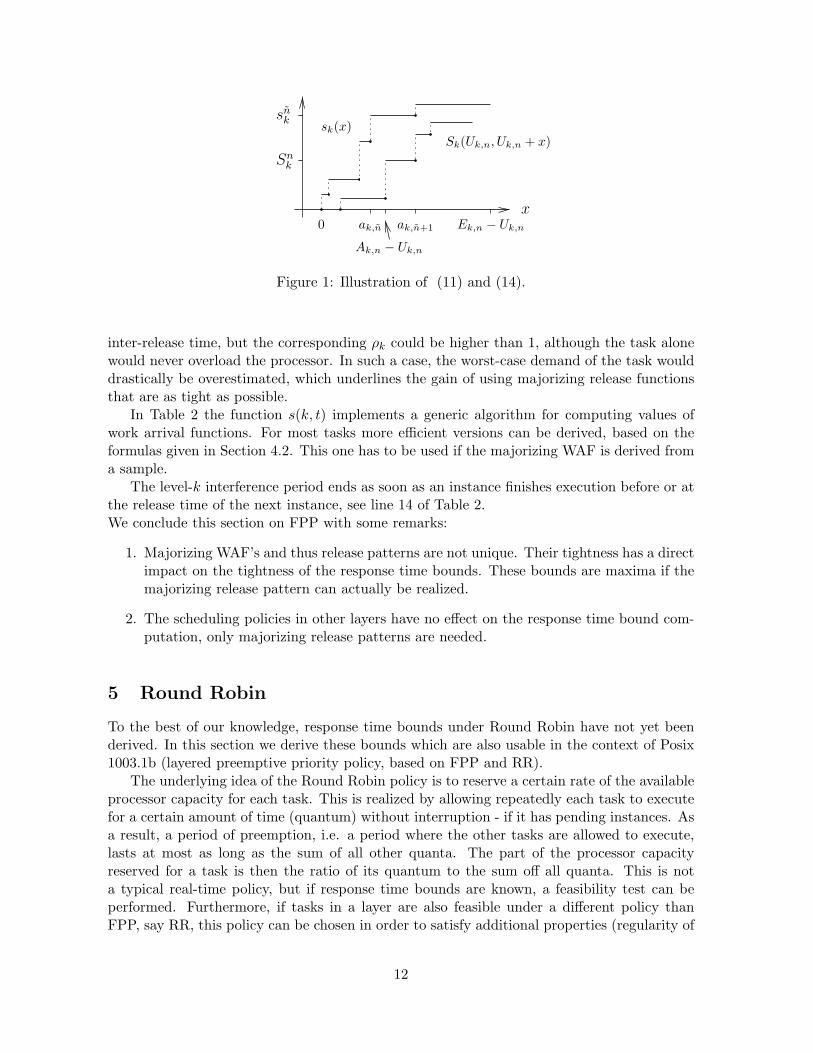
Since MWAF’s have the same properties as ordinary WAF’s, a sequence of virtual releasetimes ak,n with execution times ck,n can be found such that

sk(x) =∑n

ck,n · 1I[ak,n<x],

i.e. it can be seen as a WAF on the interval [0, x), see Figure 1. The corresponding cycletimes are tk,n = ak,n+1 − ak,n. We will refer to the set of majorizing WAF’s of tasks in Tas majorizing release pattern. The execution end of an instance of τk in the first interferenceperiod of a majorizing release pattern is of course

ek,n = min{x > 0 | s1..k−1(x) + snk = x} (12)

and the corresponding response time is

rk,n = ek,n − ak,n. (13)

The major advantage of introducing the concept of MWAF is the resulting separationof the analysis of tasks from the analysis of scheduling policies. On one hand response timeequations, which essentially depend on the scheduling policy, can be established independentlyof a particular type of task, see equation (12). On the other hand, the worst case behavior of acertain kind of task can be derived independently of the applied scheduling policy, as we haveseen in this section. This reduces the overall complexity of the timing analysis by breaking itinto separate smaller problems. In subsequent sections we apply this principle to the timinganalysis of layered priorities, by considering tasks only under the form of (majorizing) WAF,without referring to any particular kind of task.

4.3 Response time bounds

Based on the concepts of MWAF’s and interference periods defined in the previous sections,,the fundamental argument for finding response time bounds can be stated as follows.

Theorem 1Every response time of a task τk in an FPP-layer is bounded by the response time of some ofits instances in the first level-k interference period of a majorizing release pattern:

Rk,n 6 maxj=0,1,2,...,j∗

rk,j , j∗ = min{j > 0 | ek,j 6 ak,j+1}.

Proof: Let n be the index of the instance in the majorizing release pattern, that satisfies

ak,n 6 Ak,n − Uk,n < ak,n+1. (14)

Furthermore, let snk =∑n

i=0 ck,i. As illustrated in Figure 1, we have Snk 6 snk . To show this, we

have to distinguish two cases. Notice first that Snk = Sk(Uk,n, Ak,n)+Ck,n = Sk(Uk,n, Ak,n+1).

10

• Ak,n+1−Uk,n 6 ak,n+1: in this case sk(Ak,n+1−Uk,n) 6 sk(ak,n+1) since sk is increasing.With (11), we obtain

Snk = Sk(Uk,n, Ak,n+1) 6 sk(Ak,n+1 − Uk,n) 6 sk(ak,n+1) = snk .

• Ak,n+1−Uk,n > ak,n+1: in this case Sk(Uk,n, Ak,n+1) = Sk(Uk,n, Uk,n + ak,n+1), since bydefinition of n, ak,n+1 > Ak,n − Uk,n. With (11), we obtain

Snk = Sk(Uk,n, Ak,n+1) = Sk(Uk,n, Uk,n + ak,n+1) 6 sk(ak,n+1) = snk .

The execution end of τk,n is

ek,n = min{x > 0 | s1..k−1(x) + snk = x} . (15)

Inequality (11) for tasks τ1, . . . , τk−1 and Snk 6 snk implies S1..k−1(Uk,n, t)+Snk 6 s1..k−1(Uk,n−

t) + snk and hence Proposition 1 (see Appendix A) implies

Ek,n − Uk,n 6 ek,n. (16)

Now, (16) and (14) imply Rk,n 6 rk,n. So far, we have identified for each response time Rk,na bound rk,n. If we take the maximum of these bounds, we obtain a bound for all responsetimes. Recall that n is the smallest index, i.e. τk,n is the first instance, such that Snk 6 snk .Thus, to be able to determine the maximum, we need to know how large n can be.

Suppose τk,n is the first instance in a level-k interference period. In the interval [Uk,n, Ak,n)the processor is occupied by the tasks τ1, . . . , τk−1. Because of (11), the same will be true forthe majorizing release pattern during the interval [0, Ak,n − Uk,n). Since ak,n 6 Ak,n − Uk,n,τk,n is part of the first level-k interference period.

Suppose now, that τk,n is not the first instance, i.e. τk,n−1 and τk,n are part of the samelevel-k interference period, then Ek,n−1 > Ak,n. Suppose Rk,n−1 and Rk,n are both boundedby two different response times of the majorizing release pattern, i.e. suppose n− 1 < n.Then

ak,n 6 Ak,n − Uk,n < Ek,n−1 − Uk,n 6 ek,n−16 ek,n−1,

meaning that τk,n starts before τk,n−1, i.e. the bounds we are looking for are the responsetimes of instances in the first level-k interference period, remember (4). Thus we only needto compute rk,j for j = 0, 1, 2, . . . while ak,j < ek,j−1. �

An overview of the algorithm implementing this result is given in Table 2. The functionf(k, t) (on the right) returns the execution demands s1..k−1(t) on the interval [0, t). Thevariable c contains always the appropriate value of snk . Both are used in lines 5- 8 torecursively compute the execution end ek,n = min{t > 0 | f(k, t) + c = t} (see the discussionin appendix A). Convergence is guaranteed, under the following conditions of stability. Iffor each τk there exist σk, ρk ∈ R+ such that sk(x) 6 σk + ρk · x and

∑mi=1 ρi < 1 then

the majorizing release pattern is stable, which means that the processor is not overloaded inthe long run. If the majorizing pattern is based on worst-case execution and inter-releasetimes, then σk = Ck and ρk = Ck/Tk is the choice with the smallest possible value for ρk.For sporadically periodic tasks it would be σk = Nk · Ck with ρk = Nk · Ck/T

(2)k and for a

multi-frame task σk =∑Mk−1

i=0 Cik with ρk = σk/(Mk · Pk). The rate ρk is a bound on theaverage demand of a task. For a multi-frame task one could also use its worst execution and

11

Snk

x

sk(x)snk

ak,n0

Ak,n − Uk,n

ak,n+1 Ek,n − Uk,n

Sk(Uk,n, Uk,n + x)

Figure 1: Illustration of (11) and (14).

inter-release time, but the corresponding ρk could be higher than 1, although the task alonewould never overload the processor. In such a case, the worst-case demand of the task woulddrastically be overestimated, which underlines the gain of using majorizing release functionsthat are as tight as possible.

In Table 2 the function s(k, t) implements a generic algorithm for computing values ofwork arrival functions. For most tasks more efficient versions can be derived, based on theformulas given in Section 4.2. This one has to be used if the majorizing WAF is derived froma sample.

The level-k interference period ends as soon as an instance finishes execution before or atthe release time of the next instance, see line 14 of Table 2.We conclude this section on FPP with some remarks:

1. Majorizing WAF’s and thus release patterns are not unique. Their tightness has a directimpact on the tightness of the response time bounds. These bounds are maxima if themajorizing release pattern can actually be realized.

2. The scheduling policies in other layers have no effect on the response time bound com-putation, only majorizing release patterns are needed.

5 Round Robin

To the best of our knowledge, response time bounds under Round Robin have not yet beenderived. In this section we derive these bounds which are also usable in the context of Posix1003.1b (layered preemptive priority policy, based on FPP and RR).

The underlying idea of the Round Robin policy is to reserve a certain rate of the availableprocessor capacity for each task. This is realized by allowing repeatedly each task to executefor a certain amount of time (quantum) without interruption - if it has pending instances. Asa result, a period of preemption, i.e. a period where the other tasks are allowed to execute,lasts at most as long as the sum of all other quanta. The part of the processor capacityreserved for a task is then the ratio of its quantum to the sum off all quanta. This is nota typical real-time policy, but if response time bounds are known, a feasibility test can beperformed. Furthermore, if tasks in a layer are also feasible under a different policy thanFPP, say RR, this policy can be chosen in order to satisfy additional properties (regularity of

12

1 funct time RespT ime(task k)2 max := 0; n := 0; a := 0;3 c := ck,0; w := ck,0;4 repeat5 repeat6 e := w;7 w := f(k, e) + c;8 until w = e;9 r := e− a;

10 if r > max then max := r; fi11 a := a+ tk,n;12 n := n+ 1;13 c := c+ ck,n;14 until a > e;15 return max;16 end

funct time f(task k, time t)w := 0for i := 1 to k − 1 do

w := w + s(i, t);odreturn w;

end

funct time s(task i, time t)w := 0; a := 0; j := 0;while a < t do

w := w + ci,j ;a := a+ ti,j ;j := j + 1;

odreturn w;

end

Table 2: Computing a response time bound.

service, fairness, etc). This is true in particular because the alternative choice for some layerhas no effect on the response time bounds of tasks in other layers. The aim of this section isto derive bounds for tasks scheduled in a Round Robin layer under LPP and to give reasonsfor using Round Robin.

First we give a precise description of the policy. Let τk be a task in an RR-layer λl.Repeatedly, it gets the opportunity to execute during a time quantum of at most Ψk. If thetask has no pending instance or less pending work than the quantum amounts, then the rest ofthe quantum is lost for that task and it has to await the next cycle. When an instance finisheswithout completely using a quantum, then the next instance of the same task is allowed touse the rest of the quantum - if it is already pending at the time when the previous instancesis completing.

As a result, the time between two consecutive opportunities for the instances of a taskto execute may vary, depending on the actual demands of other tasks, but it is boundedby Ψl =

∑τk∈λl Ψk in any interval where the considered task has pending instances at any

moment.

5.1 Interference periods

Under RR, level-k interference periods make no sense, since any task of the layer can preemptany other. A different kind of period must be found. The discussion below shows that withthe following definition response time bounds can be found.

13

Definition 3A τk-RR-interference period is a time interval [URRk , V RR

k ) such that started instances of τk orof tasks from higher priority layers, that is τ1, . . . , τml−1

, are pending neither at its beginningURRk nor at its end V RR

k but at any other time between Uk and V k there is at least one suchinstance pending.

Such a period ends with the execution end of an instance of τk but can start with the executionbeginning of any instance of the task or of higher priority layers. At URRk started instancesof other tasks from the layer can be pending.

Furthermore, the processing unit is busy at any moment for tasks of the layer or for tasksfrom higher priority layers. For the considered task τk it implies in particular that all itsquanta which are situated inside of [URRk , V RR

k ), except for the last, are completely used, i.e.have the maximal size Ψk. To see this, suppose there is a quantum in [URRk , V RR

k ), whichis shorter than Ψk. Then, at its end an instance finishes while the next has not yet beenreleased, implying it is the end of the τk-RR-interference period.

Recall that each instance of a task in a FPP layer is part of some level-k-interferenceperiod. Here, each instance of a task is part of some τk-RR-interference period. A specialcase is that of periods containing only one quantum because the instance’s execution time isshorter than Ψk.

Basic response time bound We now turn to the timing analysis of RR. Under RR,execution times of instances are subdivided into quanta with release times that depend onRR-cycles of the scheduler in the past. RR-cycles in return depend on the way tasks actuallyused their quanta in the past. Because of this kind of feedback, an exact response-timeformula like (6) is rather complex [8]. To avoid this difficulty and because an exact formula isnot necessarily needed for finding response time bounds, we first derive a basic response timebound, for a particular instance in some interference period and adapt it in a second step tothe majorizing release pattern.

Consider therefore a τk-RR-interference period [URRk , V RRk ). As explained above, the task

τk completely uses all of the quanta the scheduler proposes to it, except perhaps for the lastone, where the last instance finishes at V RR

k . Before an instance τk,n is executed, the previousinstance τk,n−1 must first complete. Thus a total amount of Snk = Sk(URRk , Ak,n) +Ck,n unitsof work will be executed for τk in the interval [URRk , Ek,n), which corresponds to dSnk /ΨkeRR cycles. In each RR cycle the other tasks of the layer may use the processor for up toΨk = Ψl − Ψk units of time. Thus their demand in the interval [URRk , Ek,n) is bounded bydSnk /Ψke · Ψk. On the other hand it cannot exceed the actual demands, which is due toinstances of other tasks of the layer that might be pending at URRk , and the instances arrivingduring [URRk , t):

W k(URRk ) =∑

τi∈λl,τi 6=τk

Wi(URRk ) and Sk(URRk , t) =∑

τi∈λl,τi 6=τk

Si(URRk , t)

In addition, there is the demand S1..ml−1(URRk , t) from tasks in higher priority layers. Notice

that by Definition 3, W1..ml−1(URRk ) = 0. Hence the total demand of tasks other than τk is

bounded by

Ψk(URRk , t) = min( ⌈

SnkΨk

⌉·Ψk, W k(URRk ) + Sk(URRk , t)

)+ S1..ml−1

(URRk , t). (17)

14

With (17) as a bound for demands of other tasks of the layer, we deduce using Proposition 1that

Ek,n 6 E∗k,n = min{t > URRk |Ψk(URRk , t) + Snk = t− URRk }

is a bound for the actual execution end Ek,n. Thus, R∗k,n = E∗k,n − Ak,n is a bound for theresponse time Rk,n. We call R∗k,n a basic response time bound. As before we use small lettersfor the counterpart in the majorizing release pattern:

e∗k,n = min{x > 0 | ψk(x) + snk = x}. (18)

andr∗k,n = e∗k,n − ak,n. (19)

5.2 Response time Bounds

We prove in this section that the basic response time bounds in the first τk-RR-interferenceperiod of a majorizing release pattern, are also bounds for the actual response times of τk.

Theorem 2The response time of any instance τk,n in an RR-layer is bounded by the basic responsetime bound r∗k,n of some instance τk,n in the first τk-RR-interference period of the majorizingrelease pattern. Therefore:

Rk,n 6 maxj=0,1,2,...,j∗

r∗k,j where j∗ = min{j | ek,j 6 ak,j+1}.

Remark: This theorem is very similar to Theorem 1, because the method for finding responsetime bounds is basically the same. The difference lies in the specific definition of the responsetimes (basic response time bounds) and the interference periods (τk-RR-interference period).Proof: The preemption from other tasks (17) consists in two parts, which we will boundseparately. First we derive a bound for

W k(URRk ) + Sk(URRk , t) + S1..ml−1(URRk , t) . (20)

The workload W k(URRk ) is the result of the scheduling since the begin Uml of the level-ml

interference period in which τk,n is executed. At Uml there is no pending work at levelml, but at each moment until URRk there is such work pending, implying that the processoronly executes τ1, . . . , τml during [Uml , URRk ). Therefore, W1..ml(U

RRk ) = S1..ml(U

ml , URRk ) −(URRk − Uml). On the other hand,

W1..ml(URRk ) = W1..ml−1

(URRk ) +W k(URRk ) +Wk(URRk )

and by Definition 3, Wk(URRk ) = 0 and W1..mi−1(URRk ) = 0. Thus

W k(URRk ) = S1..ml(Uml , URRk )− (URRk − Uml).

Since S1..ml(Uml , URRk ) = S1..ml−1

(Uml , URRk ) + Sk(Uml , URRk ) + Sk(Uml , URRk ) and becauseof the additivity (2) of WAF’s, the term (20) becomes

W k(URRk ) + Sk(URRk , t) + S1..ml−1(URRk , t)

= Sk(Uml , URRk ) + Sk(Uml , t) + S1..ml−1(Uml , t)− (URRk − Uml)

6 sk(URRk − Uml) + sk(t− Uml) + s1..ml−1(t− Uml)− (URRk − Uml)

= sk(u) + sk(t− URRk + u) + s1..ml−1(t− URRk + u)− u. (21)

15

where we have introducing MWAF’s (11) and u = URRk − Uml . On the other hand, it iseasily seen from the identity vml = min{x > 0 | s1..ml(x) = x} and using S1..ml(U

ml , t) 6s1..ml(t − Uml), that V ml − Uml 6 vml , i.e. any level-ml interference period is shorter thanthe first level-ml period of the majorizing release pattern. Since [Uml , URRk ) ⊂ [Uml , V ml),we have therefore u = URRk − Uml 6 vml . Thus a bound for (21) is s∗k(t− URRk ), where s∗k isgiven by

s∗k(x) = max06u6vml

sk(u) + sk(u+ x) + s1..ml−1(u+ x)− u. (22)

We turn now to the other part of (17). From the definition of n, given by equation (14), itfollows immediately that⌈

SnkΨk

⌉·Ψk + S1..ml−1

(URRk , t) 6⌈snkΨk

⌉·Ψk + s1..ml−1

(t− URRk ).

Thus a bound for (17) is given by a similar expression

ψk(t− URRk ) = min(⌈

snkΨk

⌉·Ψk + s1..ml−1

(t− URRk ), s∗k(t− URRk )). (23)

From the proof of Theorem 1, we know that Ak,n > URRk + ak,n. Consider then

e∗k,n = min{x > 0 | ψk(x) + snk = x}. (24)

We call r∗k,n = e∗k,n − ak,n basic response time bound in the majorizing release pattern. Withsnk defined by (14), Proposition 1 applies to E∗k,n and e∗k,n. Thus Ek,n 6 URRk + e∗k,n, implyingfinally with (14)

Rk,n 6 E∗k,n −Ak,n 6 r∗k,n.

As in Theorem 1, it can be proven that it is sufficient to compute r∗k,j for j = 0, 1, 2, . . . whileak,j < e∗k,j−1, to determine the response time bound. �Given the MWAF’s, s∗(.) can be determined algorithmically.

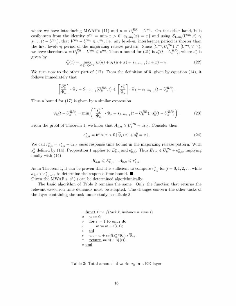
The basic algorithm of Table 2 remains the same. Only the function that returns therelevant execution time demands must be adapted. The changes concern the other tasks ofthe layer containing the task under study, see Table 3.

1 funct time f(task k, instance n, time t)2 w := 0;3 for i := 1 to ml−1 do4 w := w + s(i, t);5 od6 w := w + ceil(snk/Ψk) ∗Ψk;7 return min(w, s∗k(t));8 end

Table 3: Total amount of work: τk in a RR-layer

16

In the literature, it is sometimes claimed that SCHED RR is mainly useful for the schedul-ing of tasks in the lower priority ranges with soft timing constraints (see [14] p. 163). Onereason is perhaps the lack of schedulability analysis. Consider a subset λl of tasks thatperform some work of equal importance from the point of view of the application, such astransmitting data to other stations through the network or controlling external devices. Weclaim that if the complete set of tasks is schedulable whether SCHED RR and SCHED FIFOis used for the tasks of the subset λl, then using SCHED RR may be better.

We illustrate this with the comparison reported in Table 4. The data includes the de-scription of the tasks using symbols already introduced (except for the relative deadlines Dk),their priority level p, their response time bounds and the maximum, average and standarddeviation of the response time, obtained by simulation. Also displayed is the average CPUutilization of the task (ρk) and the cumulated utilizations of tasks with a higher or equalpriority (ρ1..k).

The response times have been computed with TkRts [15]. The column “bound” givesthe response time bounds computed by our algorithm whereas the column “max” gives themaximal response times obtained by simulation. It can be noticed that in FPP-layers themaxima are always equal to the bounds. This is due to two factors: on the one hand the FPPalgorithm actually computes maximal response times and on the other the worst-case scenariois known and was simulated (critical instant see [1]). In the case of RR-layers the boundscomputed by our algorithm are larger than the maxima obtained by simulation. There aretwo reasons: our algorithm is only able to compute upper bounds and the worst-case scenariois not known and was perhaps not simulated. In our example the difference is about 15%.

However, the use of RR has an interesting advantage: the maximum of standard deviationsof the response times in the layer λl is lower. It means that there is less “jitter” in theavailability date of the results produced by instances of task in λl. It provides, to somedegree, more predictability to the behavior of the application. In the case of distributedapplications, this may result in less bursty WAF’s and reduced response time bounds at thereceiving end.

6 Critical sections and semaphores

While a task is writing into a shared memory zone, it must not be preempted because it couldleave the zone in an incoherent state, that could then be read by another task. More generallythere are time periods, called critical sections, where a task should not be preempted by othertasks that need the same resource. To implement this, semaphores are commonly used tosignal that a resource is currently being used. But resource contentions can modify preemptivescheduling policies. Under fixed preemptive priorities it induces priority inversions: consideras an example three tasks τ1, τ2, τ3, which are given in decreasing order of priority. If afterthe beginning of a critical section of the lowest priority task τ3, the highest priority task τ1

needs the resource locked by τ3, then τ1 is blocked, which is as having a lower priority thanτ3. The medium priority task τ2 is then able to preempt τ1, by preempting the critical sectionof τ3, which is a contradiction with the intended preemptive fixed priority policy. As a result,τ1 can have longer response times than it would usually have. Normally, a transient overloadat level j, has no effect on the response times of τ1, but in the case of the priority inversionjust described, it would be blocked as long as τ2 is blocked by the execution of higher prioritytasks. A prominent example is given by the initial difficulties with the scheduler in the “Mars

17

Layer p τk Ck Tk Dk bound max mean stdev ρk ρ1..m

FPP

10 T1 3 20 20 3 3.0 3.0 0.0 15.0 15.09 T2 5 30 30 8 8.0 6.1 1.3 16.7 31.78 T3 2 40 40 10 10.0 6.1 2.7 5.0 36.77 T4 4 55 55 14 14.0 6.4 2.9 7.3 43.96 T5 7 70 70 24 24.0 12.5 4.4 10.0 53.95 T6 15 125 125 49 49.0 31.8 7.8 12.0 65.94 T7 6 150 150 55 55.0 24.4 13.2 4.0 69.93 T8 10 200 200 89 89.0 37.1 18.9 5.0 74.92 T9 11 250 250 108 108.0 70.6 17.7 4.4 79.31 T10 15 250 250 190 190.0 113.6 26.2 6.0 85.3

Layer p Ψk τk Ck Tk Dk bound max mean stdev ρk ρ1..m

FPP10 T1 3 20 20 3 3.0 3.0 0.0 15.0 15.09 T2 5 30 30 8 8.0 6.1 1.3 16.7 31.78 T3 2 40 40 10 10.0 6.1 2.7 5.0 36.7

RR

7 4 T4 4 55 50 50 46.0 10.4 6.3 7.3 43.97 7 T5 7 70 70 50 45.0 14.2 5.8 10.0 53.97 8 T6 15 125 125 89 72.0 32.3 9.1 12.0 65.97 3 T7 6 150 150 89 72.0 22.5 10.0 4.0 69.97 5 T8 10 200 200 89 72.0 27.6 11.4 5.0 74.9

FPP6 T9 11 250 250 108 108.0 70.6 17.7 4.4 79.35 T10 15 250 250 190 190.0 113.6 26.2 6.0 85.3

Table 4: Fixed priorities versus Round Robin.

18

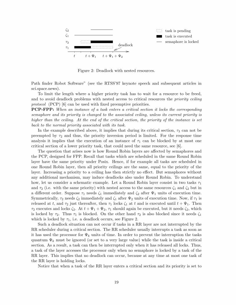
t+ Ψ1 + Ψ2t+ Ψ1t

τ1

τ2

ζ2

ζ1

deadlock

task is pendingtask is executedsemaphore is locked

Figure 2: Deadlock with nested resources.

Path finder Robot Software” (see the RTSS’97 keynote speech and subsequent articles insci.space.news).

To limit the length where a higher priority task has to wait for a resource to be freed,and to avoid deadlock problems with nested access to critical resources the priority ceilingprotocol (PCP) [6] can be used with fixed preemptive priorities.PCP-FPP: When an instance of a task enters a critical section it locks the correspondingsemaphore and its priority is changed to the associated ceiling, unless its current priority ishigher than the ceiling. At the end of the critical section, the priority of the instance is setback to the normal priority associated with its task.

In the example described above, it implies that during its critical section, τ3 can not bepreempted by τ2 and thus, the priority inversion period is limited. For the response timeanalysis it implies that the execution of an instance of τ1 can be blocked by at most onecritical section of a lower priority task, that could need the same resource, see [6].

The question that arises now is how Round Robin layers are affected by semaphores andthe PCP, designed for FPP. Recall that tasks which are scheduled in the same Round Robinlayer have the same priority under Posix. Hence, if for example all tasks are scheduled inone Round Robin layer, then all priority ceilings are the same, equal to the priority of thelayer. Increasing a priority to a ceiling has then strictly no effect. But semaphores withoutany additional mechanism, may induce deadlocks also under Round Robin. To understandhow, let us consider a schematic example. Let a Round Robin layer consist in two tasks τ1

and τ2 (i.e. with the same priority) with nested access to the same resources ζ1 and ζ2 but ina different order. Suppose τ1 needs ζ1 immediately and ζ2 after Ψ1 units of execution time.Symmetrically, τ2 needs ζ2 immediately and ζ1 after Ψ2 units of execution time. Now, if τ1 isreleased at t, and τ2 just thereafter, then τ1 locks ζ1 at t and is executed until t+ Ψ1. Thenτ2 executes and locks ζ2. At t+ Ψ1 + Ψ2, τ1 should again be executed, but it needs ζ2, whichis locked by τ2. Thus τ1 is blocked. On the other hand τ2 is also blocked since it needs ζ1

which is locked by τ1, i.e. a deadlock occurs, see Figure 2.Such a deadlock situation can not occur if tasks in a RR layer are not interrupted by the

RR scheduler during a critical section. The RR scheduler usually interrupts a task as soon asit has used the processor for Ψk units of time. In order to prevent the interruption the tasksquantum Ψk must be ignored (or set to a very large value) while the task is inside a criticalsection. As a result, a task can then be interrupted only when it has released all locks. Thus,a task of the layer accesses the processor only when no semaphore is locked by a task of theRR layer. This implies that no deadlock can occur, because at any time at most one task ofthe RR layer is holding locks.

Notice that when a task of the RR layer enters a critical section and its priority is set to

19

a ceiling that is higher than the priority of the RR layer, then it is also not interrupted bythe RR scheduler while it executes its critical section. On the other hand, if a ceiling is equalto the priority of a RR layer, the usual PCP rule is still applicable, if the RR scheduler doesnot interrupt the execution of a task whose priority would be set to the priority of the layer.

Thus, the deadlock preventing rule can more generally be stated as follows:PCP-RR.1: The time quantum of a task is ignored, while it executes a critical section.Notice that this rule may easily be implemented under Posix, by setting the time quantumto a very large value while the task executes its critical section. In Section 6.2 we deriveresponse time bounds that account for the effects of PCP-RR.1, see (28). These bounds arerather pessimistic, because with PCP-RR.1 the behavior of the policy becomes difficult toanalyse. The longer are the critical sections the less accurate is the bound (28).

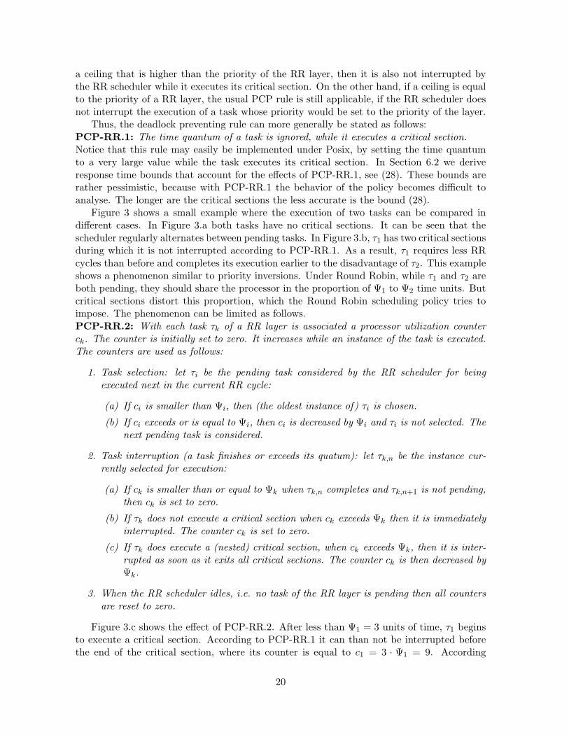
Figure 3 shows a small example where the execution of two tasks can be compared indifferent cases. In Figure 3.a both tasks have no critical sections. It can be seen that thescheduler regularly alternates between pending tasks. In Figure 3.b, τ1 has two critical sectionsduring which it is not interrupted according to PCP-RR.1. As a result, τ1 requires less RRcycles than before and completes its execution earlier to the disadvantage of τ2. This exampleshows a phenomenon similar to priority inversions. Under Round Robin, while τ1 and τ2 areboth pending, they should share the processor in the proportion of Ψ1 to Ψ2 time units. Butcritical sections distort this proportion, which the Round Robin scheduling policy tries toimpose. The phenomenon can be limited as follows.PCP-RR.2: With each task τk of a RR layer is associated a processor utilization counterck. The counter is initially set to zero. It increases while an instance of the task is executed.The counters are used as follows:

1. Task selection: let τi be the pending task considered by the RR scheduler for beingexecuted next in the current RR cycle:

(a) If ci is smaller than Ψi, then (the oldest instance of) τi is chosen.

(b) If ci exceeds or is equal to Ψi, then ci is decreased by Ψi and τi is not selected. Thenext pending task is considered.

2. Task interruption (a task finishes or exceeds its quatum): let τk,n be the instance cur-rently selected for execution:

(a) If ck is smaller than or equal to Ψk when τk,n completes and τk,n+1 is not pending,then ck is set to zero.

(b) If τk does not execute a critical section when ck exceeds Ψk then it is immediatelyinterrupted. The counter ck is set to zero.

(c) If τk does execute a (nested) critical section, when ck exceeds Ψk, then it is inter-rupted as soon as it exits all critical sections. The counter ck is then decreased byΨk.

3. When the RR scheduler idles, i.e. no task of the RR layer is pending then all countersare reset to zero.

Figure 3.c shows the effect of PCP-RR.2. After less than Ψ1 = 3 units of time, τ1 beginsto execute a critical section. According to PCP-RR.1 it can than not be interrupted beforethe end of the critical section, where its counter is equal to c1 = 3 · Ψ1 = 9. According

20

task is pending task is executed critical section

1 2 30 4 5

0

0

c1

1

21

τ2

τ1

τ2

τ1

τ2

τ1

(a) no critical sections

(b) critical sections with PCP-RR.1

(c) critical sections with PCP-RR.1 + RR.2

limit between round robin cycles

3 4

(d) counter, associated with processor usage τ1 in (c).

32

Figure 3: Critical sections under Round Robin: C1 = 15, Ψ1 = 3, C2 = 6, Ψ2 = 4.

21

to PCP-RR.2 (1.b), τ1 will not be selected by the RR scheduler in the following 2 cycles(Figure 3.d shows the evolution of the counter c1). During that time τ2 is able to ”recover”the lost quanta.

As can be seen from this example, PCP-RR.2 tends to reestablish the distorted accessrates: (c) ressembles more to (a) than (b) does.

It is possible to define the Round Robin scheduling policy in terms of time dependentpriority functions [8]. With the help of priority functions it can be seen that the PCP-RR1+2 is designed according to the same principle as the PCP [6] for FPP and the dynamicPCP [16] for Earliest deadline first.

6.1 Response time bounds of tasks in FPP-layers

We have described above how a task can preempt a higher priority task by executing itscritical section. The PCP does not prevent this from happening. Its aim is to limit theduration of such periods. It has been shown in [6] that under the FPP policy with PCP,during a level-k busy period a task τk can be preempted by only one critical section of a lowerpriority task. Since interference periods are sub-intervals of busy periods, the same holds truefor them. To account for critical sections the execution end formula (6) changes to

Ek,n = min{t > Uk,n | S1..k−1(Uk,n, t) +Bk,n + Snk = t− Uk,n} (25)

with Bk,n being the length of the unique preempting critical section if it exists and Bk,n = 0otherwise. Its value is bounded by the maximum length of critical sections of lower prioritytask that can lock the same semaphores as τk. This maximum is denoted bk. Thus, theformula of execution end bounds needs to be changed to

ek,n = min{t > 0 | s1..k−1(t) + bk + snk = t}. (26)

From the point of view of a task in a FPP-layer, tasks with critical sections in lower priorityRR-layers behave exactly like other lower priority tasks, because of PCP-RR.1. PCP-RR.2only concerns tasks in RR-layers. Since (25) is still valid for a task in a FPP-layer, (26) givesa response time bound.

6.2 Response time bounds for tasks in RR-layers

PCP-RR.1 implies that a task τi may use the processor for more than Ψi units of time withoutinterruption if it has critical sections. If τi starts to execute a critical section just before itsquantum expires, then it may use the processor for up to Ψi + zi units of time. It depends onthe number and locations of the critical sections in the code of τi, when the task is actuallyusing the processor for longer than foreseen by RR. It is therefore difficult to exactly accountfor the resulting effect on the response time of an other task of the RR layer. A response timebound may nevertheless be obtained by assuming a pessimistic case where each other taskuses the processor during Ψi + zi units of time in each RR cycle but the task τk under studyonly for during Ψk units. It is an acceptable overestimation if zi is relatively small comparedto Ψi.

The blocking factor bk is the same for all tasks in the Round Robin layer. It is the longestcritical section of a task with a lower priority than the layer and due to a resource which isalso needed by tasks of the RR layer or higher priority layers. For the critical sections of the

22

RR layer, we introduce zk =∑

τi∈λl,τi 6=τk zi. Thus, a response time bound is obtained fromthe (pessimistic) execution end:

e∗k,n = min{x > 0 | ψk(x) + bk + snk = t} (27)

with

ψk(x) = min(⌈

snkΨk

⌉·(Ψk + zk

)+ s1..ml−1(x), s∗k(x)

). (28)

The effect of PCP-RR.2 is that when a task τi uses the processor during Ψi + zi units oftime in a single RR cycle, then it is not allowed to use the following quanta until the excessis compensated. It implies that it can only enter a critical section when it has not used theprocessor more than allowed in the past.

Suppose a task τi executes a critical section in the jth RR cycle after URRk . According toPCP-RR.2, at beginning of this cycle, τi has used the processor for at most (j − 1) ·Ψi unitsof time and at the end of the RR cycle, for at most zi + j ·Ψi. If in the jth RR cycle τi is notinside a critical section then it has used the processor for at most j ·Ψi units of time at theend of the cycle. Thus,

ψk(x) = min(⌈

snkΨk

⌉·Ψk + zk + s1..ml−1(x), s∗k(x)

). (29)

Notice that the blocking factor bk appears as an isolated additional constant in equation (27).With PCP-RR.2, the same is true for zk, which accounts for the critical sections of the tasksin the RR layer.

7 Case-study

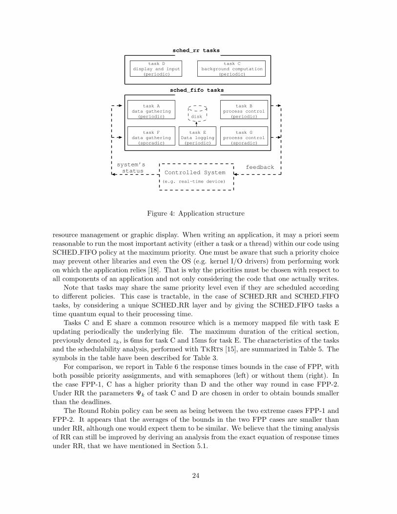
We will consider an application, running on a uniprocessor machine with a Posix 1003.1bcompliant OS, that monitors and controls a real-time device (inspired from [14] p. 152, seeFigure 4). The aim of this case study is to demonstrate that a timing analysis of a complexRR/FPP interaction is indeed possible. For a more detailed study the reader is referredto [17].

The application is structured as 7 tasks. The informations on the controlled system’sstate are gathered by task A. Task B analyses the data, takes the appropriate decisions andsends them back to the controlled system. Task C is a background computation task thatkeeps statistics up to date or implements some artificial intelligence techniques. Informationson the system’s state evolution are displayed by task D and logged onto a file by task E. TaskD also takes care of user input. In the case of an abnormal system state, an alarm conditionis triggered and task F is executed for urgent data collecting, task G will then take decisionsand send back the control data to the system. Each task is either periodic or sporadic witha worst-case time between successive invocations and each task owns a scheduling policywith a given priority fixed for the entire system’s lifetime. In this case-study, in order to stayconsistent with the notations from the previous sections, we will adopt the priority numberingscheme “the smaller the number, the higher the priority” which is the inverse of Posix.

In the development process of a real application, one is likely to be working with librariesfrom third-part suppliers or from the OS vendor for functions like network communication,

23

task Adata gathering

(periodic)

sched_fifo tasks

sched_rr tasks

task Ddisplay and input

(periodic)

Controlled System

task EData logging(periodic)

disk

task Cbackground computation

(periodic)

task Fdata gathering

(sporadic)

task Bprocess control

(periodic)

task Gprocess control

(sporadic)

feedbacksystem’s status

(e.g. real-time device)

Figure 4: Application structure

resource management or graphic display. When writing an application, it may a priori seemreasonable to run the most important activity (either a task or a thread) within our code usingSCHED FIFO policy at the maximum priority. One must be aware that such a priority choicemay prevent other libraries and even the OS (e.g. kernel I/O drivers) from performing workon which the application relies [18]. That is why the priorities must be chosen with respect toall components of an application and not only considering the code that one actually writes.

Note that tasks may share the same priority level even if they are scheduled accordingto different policies. This case is tractable, in the case of SCHED RR and SCHED FIFOtasks, by considering a unique SCHED RR layer and by giving the SCHED FIFO tasks atime quantum equal to their processing time.

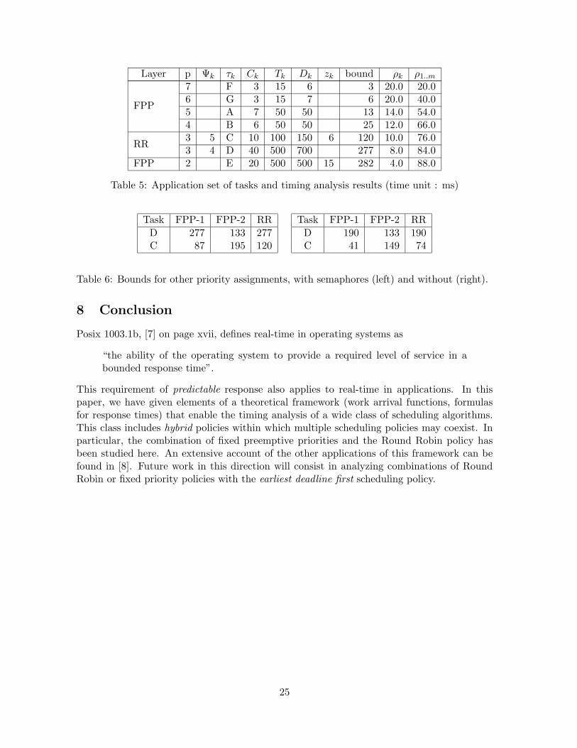
Tasks C and E share a common resource which is a memory mapped file with task Eupdating periodically the underlying file. The maximum duration of the critical section,previously denoted zk, is 6ms for task C and 15ms for task E. The characteristics of the tasksand the schedulability analysis, performed with TkRts [15], are summarized in Table 5. Thesymbols in the table have been described for Table 3.

For comparison, we report in Table 6 the response times bounds in the case of FPP, withboth possible priority assignments, and with semaphores (left) or without them (right). Inthe case FPP-1, C has a higher priority than D and the other way round in case FPP-2.Under RR the parameters Ψk of task C and D are chosen in order to obtain bounds smallerthan the deadlines.

The Round Robin policy can be seen as being between the two extreme cases FPP-1 andFPP-2. It appears that the averages of the bounds in the two FPP cases are smaller thanunder RR, although one would expect them to be similar. We believe that the timing analysisof RR can still be improved by deriving an analysis from the exact equation of response timesunder RR, that we have mentioned in Section 5.1.

24

Layer p Ψk τk Ck Tk Dk zk bound ρk ρ1..m

FPP

7 F 3 15 6 3 20.0 20.06 G 3 15 7 6 20.0 40.05 A 7 50 50 13 14.0 54.04 B 6 50 50 25 12.0 66.0

RR3 5 C 10 100 150 6 120 10.0 76.03 4 D 40 500 700 277 8.0 84.0

FPP 2 E 20 500 500 15 282 4.0 88.0

Table 5: Application set of tasks and timing analysis results (time unit : ms)

Task FPP-1 FPP-2 RRD 277 133 277C 87 195 120

Task FPP-1 FPP-2 RRD 190 133 190C 41 149 74

Table 6: Bounds for other priority assignments, with semaphores (left) and without (right).

8 Conclusion

Posix 1003.1b, [7] on page xvii, defines real-time in operating systems as

“the ability of the operating system to provide a required level of service in abounded response time”.

This requirement of predictable response also applies to real-time in applications. In thispaper, we have given elements of a theoretical framework (work arrival functions, formulasfor response times) that enable the timing analysis of a wide class of scheduling algorithms.This class includes hybrid policies within which multiple scheduling policies may coexist. Inparticular, the combination of fixed preemptive priorities and the Round Robin policy hasbeen studied here. An extensive account of the other applications of this framework can befound in [8]. Future work in this direction will consist in analyzing combinations of RoundRobin or fixed priority policies with the earliest deadline first scheduling policy.

25

References

[1] C.L. Liu and J.W. Layland. Scheduling algorithms for multiprogramming in hard real-time environment. Journal of the ACM, 20(1):40–61, February 73.

[2] J. Lehozky, L. Sha, and Y. Ding. The rate monotonic scheduling algorithm: Exactcharacterization and average case behavior. In Proceedings IEEE Real-Time SystemsSymposium, pages 166–171, December 1989.

[3] M. Joseph and P Pandya. Finding response times in a real-time system. The ComputerJournal, 29(5):390–395, 1986.

[4] J.P. Lehoczky. Fixed priority scheduling of periodic task sets with arbitrary deadlines. InProceedings of the 11th IEEE Real-Time Systems Symposium, pages 201–209, December1990.

[5] K. Tindell, A. Burns, and A.J. Wellings. An extendible approach for analysing fixedpriority hard real time sytems. Real-Time Systems, 6(2), 1994.

[6] L. Sha, R. Rajkumar, and J.P. Lehoczky. Priority inheritance protocols: An approach toreal-time synchronization. IEEE Transactions on Computers, 39(9):1175–1185, Septem-ber 1990.

[7] (ISO/IEC). 9945-1:1996 (ISO/IEC)[IEEE/ANSI Std 1003.1 1996 Edition] InformationTechnology - Portable Operating System Interface (POSIX) - Part 1 : System Applica-tion : Program Interface. IEEE Standards Press, 1996. ISBN 1-55937-573-6.

[8] J. Migge. Scheduling of recurrent tasks on one processor: A trajectory based Model. PhDthesis, Universite Nice Sophia-Antipolis, 1999. http://www.migge.net/jorn/thesis/.

[9] A. Mok and D. Chen. A multiframe model for real-time tasks. IEEE Transactions onSoftware Engineering, 23(10):635–645, oktober 1997.

[10] L. George, N. Rivierre, and M. Spuri. Preemptive and non-preemptive real-time uni-processor scheduling. Technical Report 2966, INRIA, september 1996.

[11] P. Pushner. Worst-case execution-time analysis at low cost. Control Eng. Practice,6:129–135, 1998.

[12] C.Y. Park. Predicting program execution times by analyzing static and dynamic pro-grams paths. Real-Time Systems, 5(1):31–62, 1993.

[13] K.W. Tindell. Fixed Priority Scheduling of Hard Real-Time Systems. PhD thesis, Uni-versity of York, December 1993.

[14] B.O. Gallmeister. Programming for the Real World - Posix 4. O’Reilly & Associates,1995. ISBN 1-56592-074-0.

[15] J. Migge. Tkrts: A tool for computing response time bounds with a trajectory basedmodel., 1998. http://www.migge.net/jorn/rts/.

[16] M. Chen and K. Lin. Dynamic priority ceiling: A concurrency control protocol forreal-time systems. RTS, 2, 1990.

26

[17] N. Navet and J.M. Migge. Fine tuning the scheduling of tasks onposix1003.1b compliant systems. Research Report 3730, INRIA, 1999.ftp://ftp.inria.fr/INRIA/publication/RR/RR-3730.ps.gz.

[18] D.R. Butenhof. Programming with POSIX Threads. Addison-Wesley, 1997.

27

A Fixed point equations and response time bounds

It has been shown above that response times can be expressed as particular solutions of fixedpoint equations. These equations generally have more than one fixed point such that in theirneighborhood, the involved function is not necessarily a contraction. This partially explainswhy response times appear as “first fixed point after some point”, see (30).

Let x0 ∈ R and f be a function R 7−→ R with f(x0) > 0 such that

x1 = min{x > x0 | f(x) = x− x0 } (30)

exists. If f can be bounded by another function f then the first fixed point either remainsunchanged or is shifted towards the future, seen relative to their respective reference pointsx0 and 0:

Proposition 1Let f be a function R 7−→ R with f(x0) > 0 such that

x1 = min{x > 0 | f(x) = x } (31)

exists and∀ x ∈ [x0, x1) f(x) 6 f(x− x0). (32)

Then x1 − x0 6 x1

Proof: Equation (30) and (32) imply

∀ x ∈ [x0, x1) x− x0 < f(x) 6 f(x− x0)

and thus x1 6∈ [0, x1 − x0). �This is typically used when deriving response time bounds with x0 = Uk,n being the

beginning of the interference period containing the instance under study and the beginningu = 0 of the first interference period of the majorizing release pattern: Ek,n − Uk,n 6 rk,n.

28

B Notations

Ak,n activation or release time of τk,nbk maximum length of critical sections of lower priority task

that can lock the same semaphores as τk.ak,n, ck,n activation and execution times in the worst case activation patternCk,n execution time of τk,nEk,n execution end of τk,nλl layer = subset of tasks τml−1

, τml−1+1, τml−1+2, . . . , τmlml index of the last task in λlΨk time quantum for τk under Round RobinΨl sum of the quanta of the tasks in layer λl.Ψk sum of the quanta of the task in layer λl except that of τk.Si(t1, t2) work due to instances of τi activated in [t1, t2): work arrival function (WAF)S1..i(t1, t2) work due to instances of τ1, . . . , τi activated in [t1, t2)Snk work due to instances of τk in [Uk,n, Ak,n).si(x) work due to instances of τi activated in [0, x) of the worst case pattern: (MWAF)s1..i(x) work due to instances of τ1, . . . , τi activated in [0, x) of the worst case patternsnk bound for Snk derived from sk(x).Sk(t1, t2) work due to tasks of τk’s layer other than τk, activated in [t1, t2)Tk,n inter-arrival time Tk,n+1 − Tk,nT task setτk task number kτk,n nth instance or release of τkUk,n beginning of the level-k interference period containing Ak,nUk beginning of a level-k interferenceURRk beginning of a τk-RR-interference periodVk,n end of the level-k interference period containing Ak,nV k end of a level-k interferenceV RRk end of a τk-RR-interference periodWk(t) pending work at t, due to instances of τk activated strictly before t.W1..ml(t) pending work at t, due to instances of τ1, τ2 . . . , τml activated strictly before t.W k(t) pending work at t, due to instances of the task in a RR-layer except that of τk.zk longest critical section of τk

C Acronyms

FPP Fixed Preemptive PrioritiesLPP Layered Preemptive PrioritiesRR Round RobinWAF Work Arrival FunctionMWAF Majorizing Work Arrival FunctionPOSIX Portable Operating System InterfaceWCET Worst Case Execution Time

29