Embed Size (px)
Citation preview
Digital Signal Processing 22 (2012) 1010–1023
Contents lists available at SciVerse ScienceDirect
Digital Signal Processing
www.elsevier.com/locate/dsp
Time–frequency analysis of signals using support adaptive Hermite–Gaussianexpansions
Yasar Kemal Alp a,b,∗, Orhan Arıkan a
a Department of Electrical and Electronics Engineering, Bilkent University, Ankara TR-06800, Turkeyb Radar, Electronic Warfare and Intelligence Systems Division, ASELSAN A.S, Ankara TR-06370, Turkey
a r t i c l e i n f o a b s t r a c t
Article history:Available online 18 May 2012
Keywords:Hermite–Gaussian functionOrthonormal basisTime–frequency supportSignal component
Since Hermite–Gaussian (HG) functions provide an orthonormal basis with the most compact time–frequency supports (TFSs), they are ideally suited for time–frequency component analysis of finite energysignals. For a signal component whose TFS tightly fits into a circular region around the origin, HGfunction expansion provides optimal representation by using the fewest number of basis functions.However, for signal components whose TFS has a non-circular shape away from the origin, straightforward expansions require excessively large number of HGs resulting to noise fitting. Furthermore, forclosely spaced signal components with non-circular TFSs, direct application of HG expansion cannotprovide reliable estimates to the individual signal components. To alleviate these problems, by usingexpectation maximization (EM) iterations, we propose a fully automated pre-processing technique whichidentifies and transforms TFSs of individual signal components to circular regions centered around theorigin so that reliable signal estimates for the signal components can be obtained. The HG expansionorder for each signal component is determined by using a robust estimation technique. Then, theestimated components are post-processed to transform their TFSs back to their original positions.The proposed technique can be used to analyze signals with overlapping components as long as theoverlapped supports of the components have an area smaller than the effective support of a Gaussianatom which has the smallest time-bandwidth product. It is shown that if the area of the overlapregion is larger than this threshold, the components cannot be uniquely identified. Obtained results onthe synthetic and real signals demonstrate the effectiveness for the proposed time–frequency analysistechnique under severe noise cases.
© 2012 Elsevier Inc. All rights reserved.
1. Introduction
Since Hermite–Gaussian (HG) functions constitute a natural ba-sis for signals with compact time–frequency supports (TFSs), theyhave found applications in various fields of signal processing. Inimage processing, Hermite transform has been proposed for cap-turing local information [1]. Another image processing applicationis given in [2] for rotation of images. Also, in [3], HG functions areused for reconstruction of video frames. In telecommunications,highly localized pulse shapes both in time and frequency domainscan be generated by using linear combinations of the HG func-tions [4]. As part of biomedical applications, representation of EEGand ECG signals in terms of HGs also have been proposed [5,6].In [7], HG functions are used for characterization of the origins ofvibrations in swallowing accelerometry signals. An electromagnet-
* Corresponding author at: Department of Electrical and Electronics Engineering,Bilkent University, Ankara TR-06800, Turkey.
E-mail addresses: [email protected] (Y.K. Alp), [email protected](O. Arıkan).
1051-2004/$ – see front matter © 2012 Elsevier Inc. All rights reserved.http://dx.doi.org/10.1016/j.dsp.2012.05.005
ics application is reported in [8], where the time domain responseof a three-dimensional conducting object excited by a compactTFS function is modeled by using HG expansions to obtain a fastextrapolator based on this expansion. Another electromagneticsapplication reported in [9], where a new method for evaluatingdistortion in multiple waveform sets in UWB communications hasbeen proposed. Finally, as signal processing applications, HG func-tions are used for designing high resolution, multi-window time–frequency representation, where different order HGs are employedto realize multiple windows, and non-stationary spectrum estima-tion [10–13].
Single or multi-component signals with compact TFSs are fre-quently encountered in radar, sonar, seismic, acoustic, speech andbiomedical signal processing applications [14–19]. Decompositionof such a signal into its components is an important applicationof time–frequency analysis [20]. For signals whose componentshave generalized time–bandwidth products of around 1, waveletand chirplet based signal analysis techniques have been developed[21–23].
In this work, we are proposing a new signal analysis techniquefor signals whose components may have larger time-bandwidth
Y.K. Alp, O. Arıkan / Digital Signal Processing 22 (2012) 1010–1023 1011
products. Such signals are commonly employed in electronic war-fare, including radar and sonar applications, because of their highresolution properties. Furthermore, biomedical signals includingEEG and ECG have complicated time–frequency structures thatsignificantly benefits from the proposed approach. The proposedtechnique makes use of adaptive HG basis expansion to estimateindividual signal components. It is a well-known fact that HG func-tions form an orthonormal basis for the space of finite energysignals which are piecewise smooth in every finite interval [24].What makes HGs special among other types of basis functions istheir optimal localization properties in both time and frequencydomains. For any circular TFS around the origin, HGs provide thehighest energy concentration inside that region [25–27]. There-fore, if a signal component has a circular TFS around the origin,its representation by using the HG basis provides the optimal rep-resentation for a given number of representation order. However,if the signal component has a non-circular TFS positioned awayfrom the origin, its HG representation is no longer optimal. Here,we propose an adaptive pre-processing stage where TFS of the sig-nal component is transformed to a circular one centered aroundthe origin so that it can be efficiently represented by HGs. The ex-pansion order is estimated by a noise penalized costm function.Then, the desired representation is obtained by back transformingthe identified signal component. For signals with multiple com-ponents that do not have overlapping TFSs, an EM based iterativeprocedure is proposed for joint analysis and expansion of individ-ual signal components in HG basis.
The outline of the presentation is as follows. In Section 2, wegive a brief review of HG functions and emphasize their fundamen-tal properties. In Section 3, the proposed pre-processing stage isintroduced. EM based iterative component estimation for analysisof multi-component signals and determination of optimal expan-sion orders are explained in Section 4. Results on synthetic andreal signals are provided in Section 5. Conclusions are given in Sec-tion 6.
Note that, unless otherwise is stated, the integrals are com-puted in the (−∞,∞) interval. Bold characters denote vectors,(.)H and (.)∗ are used for vector Hermitian and complex conju-gation operations.
2. Review of Hermite–Gaussian functions
HG functions form a family of solutions to the following non-linear differential equation:
f ′′(t) + 4π2(
2n + 1
2π− t2
)f (t) = 0. (1)
The nth order HG function hn(t) is related to the nth order Hermitepolynomial Hn(t) as
hn(t) = 21/4
√2nn! Hn(
√2πt)e−πt2
, (2)
where, with the initialization of H0(t) = 1 and H1(t) = 2t , Hn(t)can be recursively obtained as
Hn+1(t) = 2t Hn(t) − 2nHn−1(t). (3)
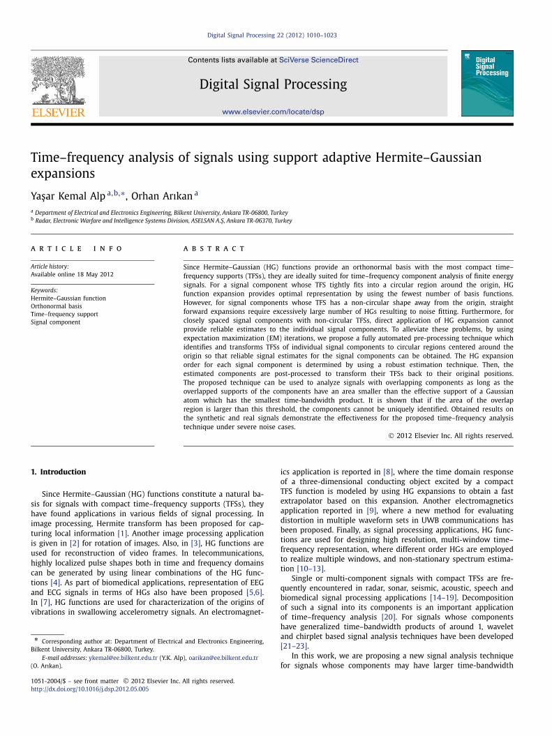
Therefore, HG functions can also be computed recursively. A de-tailed discussion on HG functions and Hermite polynomials areavailable in [28] and [29], respectively. HG functions, of which thefirst four are shown in Fig. 1, form an orthonormal basis for thespace of finite energy signals which are piecewise smooth in everyfinite [−τ , τ ] interval [24]. Hence, if s(t) is in this space, it can berepresented as
Fig. 1. The first four HG functions: (a) h0(t); (b) h1(t); (c) h2(t); (d) h3(t).
s(t) =∞∑
n=0
αnhn(t), (4)
where the expansion coefficients are
αn =∫
hn(t)s(t)dt. (5)
Furthermore, HG functions are eigenvectors of the Fourier transfor-mation [30]:
F{
hn(t)} = λnhn(t), (6)
where F is the Fourier transform operator defined as F{s(t)} =∫s(t)e− j2π f t dt and λn = e− j π
2 n is its nth eigenvalue. Similarly, thefractional Fourier transform (FrFT) of order −2 � a < 2, also admitsthe HG functions as its eigenfunctions [31]:
Fa{hn(t)} = e− j π
2 anhn(t), (7)
where Fa is the FrFT operator of order a. Hence, FrFT of s(t) can beobtained as:
Fa{s(t)} =
∞∑n=0
αne− j π2 anhn(t). (8)
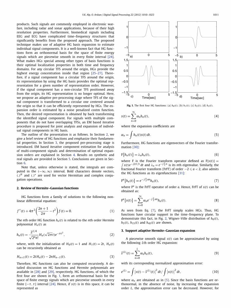
As seen from Eq. (7), the FrFT simply scales HGs. Thus, HGfunctions have circular support in the time–frequency plane. Todemonstrate this fact, in Fig. 2, Wigner–Ville distribution of h0(t),h5(t), h15(t) and h45(t) are shown.
3. Support adaptive Hermite–Gaussian expansion
A piecewise smooth signal s(t) can be approximated by usingthe following Lth order HG expansion:
s(L)(t) =L∑
n=0
αnhn(t), (9)
with its corresponding normalized approximation error:
e(L) =∫ ∣∣s(t) − s(L)(t)
∣∣2dt/
∫ ∣∣s(t)∣∣2dt, (10)
where αn are obtained as in (5). Since the basis functions are or-thonormal, in the absence of noise, by increasing the expansionorder L, the approximation error can be decreased. However, for
1012 Y.K. Alp, O. Arıkan / Digital Signal Processing 22 (2012) 1010–1023
Fig. 2. Wigner–Ville distribution of (a) h0(t); (b) h5(t); (c) h15(t); (d) h45(t).
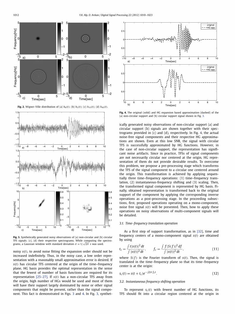
Fig. 3. Synthetically generated noisy observations of (a) non-circular and (b) circularTFS signals; (c), (d) their respective spectrograms. While computing the spectro-grams, a Gaussian window with standard deviation σ = 1/
√2π s was used.
noisy s(t), to avoid noise fitting the expansion order should not beincreased indefinitely. Thus, in the noisy case, a low order repre-sentation with a reasonably small approximation error is desired. Ifs(t) has circular TFS centered at the origin of the time–frequencyplane, HG basis provides the optimal representation in the sensethat the fewest of number of basis functions are required for itsrepresentation [25–27]. If s(t) has a non-circular TFS away fromthe origin, high number of HGs would be used and most of themwill have their support largely dominated by noise or other signalcomponents that might be present, rather than the signal compo-nent. This fact is demonstrated in Figs. 3 and 4. In Fig. 3, synthet-
Fig. 4. The original (solid) and HG expansion based approximation (dashed) of the(a) non-circular support and (b) circular support signal shown in Fig. 3.
ically generated noisy observations of non-circular support (a) andcircular support (b) signals are shown together with their spec-trograms provided in (c) and (d), respectively. In Fig. 4, the actualnoise-free signal components and their respective HG approxima-tions are shown. Even at this low SNR, the signal with circularTFS is successfully approximated by HG functions. However, inthe case of non-circular support, the representation has signifi-cant noise artifacts. Since in practice, TFSs of signal componentsare not necessarily circular nor centered at the origin, HG repre-sentation of them do not provide desirable results. To overcomethis problem, we propose a pre-processing stage which transformsthe TFS of the signal component to a circular one centered aroundthe origin. This transformation is achieved by applying sequen-tially three time–frequency operations: (1) time–frequency trans-lation, (2) instantaneous-frequency shifting and (3) scaling. Then,the transformed signal component is represented by HG basis. Fi-nally, obtained representation is transformed back to the originalsupport of the component by applying the corresponding inverseoperations as a post-processing stage. In the proceeding subsec-tions, first, proposed operations operating on a mono-component,noise free signal s(t) will be presented. Then, how to apply theseoperations on noisy observations of multi-component signals willbe detailed.
3.1. Time–frequency translation operation
As a first step of support transformation, as in [32], time andfrequency centers of a mono-component signal s(t) are obtainedby using
tc =∫
t|s(t)|2 dt∫ |s(t)|2 dt, fc =
∫f |S( f )|2 df∫ |s(t)|2 dt
, (11)
where S( f ) is the Fourier transform of s(t). Then, the signal istranslated in the time–frequency plane so that its time–frequencycenter is at the origin:
sc(t) = s(t + tc)e− j2π fct . (12)
3.2. Instantaneous frequency shifting operation
To represent sc(t) with fewest number of HG functions, itsTFS should fit into a circular region centered at the origin in
Y.K. Alp, O. Arıkan / Digital Signal Processing 22 (2012) 1010–1023 1013
the time–frequency plane. This means that, the generalized time-bandwidth product (GTBP) of the translated signal sc(t) should beminimized [21]. GTBP of sc(t) can be minimized by shifting its in-stantaneous frequency (IF) to the dc level for all time instants. IFof sc(t) can be computed as
fc(t) =∫
f W sc (t, f )df∫W sc (t, f )df
, (13)
where W sc (t, f ) is the Wigner–Ville distribution of sc(t) [32]. Notethat since sc(t) is mono-component and noise free, computed fc(t)is the true instantaneous frequency of sc(t). Then, IF shifting oper-ation is applied to sc(t) as:
sφ(t) = sc(t)e− j2πφc(t), (14)
where φc(t) is the instantaneous phase of sc(t) defined as the cu-mulative IF function [32]:
φc(t) =t∫
−∞fc(τ )dτ . (15)
3.3. Scaling operation
Once time–frequency translation and IF shifting operations areapplied to s(t), it should be scaled by a proper scaling factor sothat its effective duration and bandwidth are equalized. Effectiveduration and bandwidth of sφ(t) are defined as [32]:
Dφ =[∫
(t − tφ)2|sφ(t)|2 dt∫ |sφ(t)|2 dt
]1/2
, (16)
Bφ =[∫
( f − fφ)2|Sφ( f )|2 df∫ |sφ(t)|2 dt
]1/2
, (17)
where Sφ( f ) is the Fourier transform of sφ(t), tφ and fφ are, re-spectively, time and frequency centers of the sφ(t) given by
tφ =∫
t|sφ(t)|2 dt∫ |sφ(t)|2 dt, fφ =
∫f |Sφ( f )|2 df∫ |sφ(t)|2 dt
. (18)
Effective duration and bandwidth of sφ(tν) are equalized by choos-ing the scaling factor ν as:
ν = √Dφ/Bφ. (19)
Following this scaling, effective duration and bandwidth of sφ(tν)
are both equal to√
Dφ Bφ . After applying the scaling operation, weget:
ss(t) = s(tν + tc)e− j2πφ(tν+tc). (20)
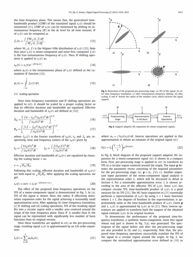
The effect of the proposed time–frequency operations on theTFS of a mono-component signal is demonstrated in Fig. 5. In (a),TFS of the signal is shown. Here, the radius R effectively deter-mines expansion order for the signal achieving a reasonably smallapproximation error. After applying (b) time–frequency translation,(c) IF shifting and (d) scaling operations, TFS of the resulting signalfits into a circular region with a smaller area centered around theorigin of the time–frequency plane. Since R ′ is smaller than R , thesignal can be represented with significantly less number of basisfunctions than its original version.
Once these transforms are applied to s(t) as the pre-processingstage, resulting signal ss(t) is approximated by an Lth order expan-sion:
ss(t) =L∑
αnhn(t), (21)
n=0Fig. 5. Illustration of the proposed pre-processing stage: (a) TFS of the signal; (b) af-ter time–frequency translation; (c) after instantaneous frequency shifting; (d) afterscaling. R and R ′ denote the radius of the smallest circle, which encloses the signalsupport.
Fig. 6. Support adaptive HG expansion for mono-component signals.
where αn = ∫hn(t)ss(t)dt . Inverse operations are applied to this
approximation to obtain an estimate of the original signal s(t):
s(t) = ss
(t − tc
ν
)e j2πφ(t). (22)
In Fig. 6, block diagram of the proposed support adaptive HG ex-pansion for a mono-component signal s(t) is shown in a compactform. First, pre-processing stage is applied to s(t) to transform itsTFS to a circular region centered around the origin. The input p de-notes the parameter vector consisting of the required parametersfor the pre-processing stage, i.e., p = {tc, f (t), v}. Another impor-tant input parameter of the mono-component signal analysis isthe representation order L, which will be discussed in detail inSection 4. For a reasonable approximation error, L is chosen ac-cording to the area of the effective TFS of ss(t). Since ss(t) hascompact circular TFS, time-bandwidth product of ss(t) is a goodmeasure for its TFS [21]. The HG basis expansion in (21) essentiallyperforms a representation of ss(t) by using L + 1 basis functionswhere L + 1, the degrees of freedom in the representation, is ap-proximately same as the time-bandwidth product of ss(t). Given pand L, ss(t) is approximated by ss(t) as in (21). Then, inverse op-erations are applied to transform back the support of the obtainedsignal estimate ss(t) to its original location.
To demonstrate the performance of the proposed time-fre-quency transforms, a synthetic mono-component, noise free signalwhose real part is shown in Fig. 7(a), was generated. The spec-trogram of the signal before and after the pre-processing stageare also provided in (b) and (c), respectively. Note that, the pro-posed time–frequency operations successfully translate the TFS ofthe signal to a circular region around the origin. In Fig. 8, wecompare the normalized approximation error defined in (10) as
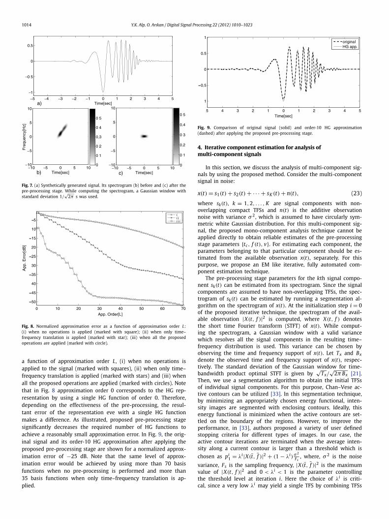
1014 Y.K. Alp, O. Arıkan / Digital Signal Processing 22 (2012) 1010–1023
Fig. 7. (a) Synthetically generated signal. Its spectrogram (b) before and (c) after thepre-processing stage. While computing the spectrogram, a Gaussian window withstandard deviation 1/
√2π s was used.
Fig. 8. Normalized approximation error as a function of approximation order L:(i) when no operations is applied (marked with square); (ii) when only time–frequency translation is applied (marked with star); (iii) when all the proposedoperations are applied (marked with circle).
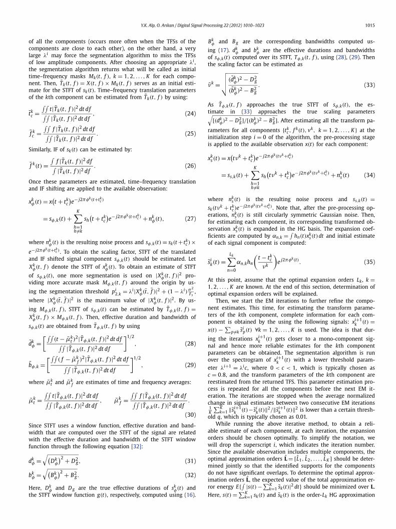
a function of approximation order L, (i) when no operations isapplied to the signal (marked with squares), (ii) when only time–frequency translation is applied (marked with stars) and (iii) whenall the proposed operations are applied (marked with circles). Notethat in Fig. 8 approximation order 0 corresponds to the HG rep-resentation by using a single HG function of order 0. Therefore,depending on the effectiveness of the pre-processing, the resul-tant error of the representation eve with a single HG functionmakes a difference. As illustrated, proposed pre-processing stagesignificantly decreases the required number of HG functions toachieve a reasonably small approximation error. In Fig. 9, the orig-inal signal and its order-10 HG approximation after applying theproposed pre-processing stage are shown for a normalized approx-imation error of −25 dB. Note that the same level of approx-imation error would be achieved by using more than 70 basisfunctions when no pre-processing is performed and more than35 basis functions when only time–frequency translation is ap-plied.
Fig. 9. Comparison of original signal (solid) and order-10 HG approximation(dashed) after applying the proposed pre-processing stage.
4. Iterative component estimation for analysis ofmulti-component signals
In this section, we discuss the analysis of multi-component sig-nals by using the proposed method. Consider the multi-componentsignal in noise:
x(t) = s1(t) + s2(t) + · · · + sK (t) + n(t), (23)
where sk(t), k = 1,2, . . . , K are signal components with non-overlapping compact TFSs and n(t) is the additive observationnoise with variance σ 2, which is assumed to have circularly sym-metric white Gaussian distribution. For this multi-component sig-nal, the proposed mono-component analysis technique cannot beapplied directly to obtain reliable estimates of the pre-processingstage parameters {tc, f (t), v}. For estimating each component, theparameters belonging to that particular component should be es-timated from the available observation x(t), separately. For thispurpose, we propose an EM like iterative, fully automated com-ponent estimation technique.
The pre-processing stage parameters for the kth signal compo-nent sk(t) can be estimated from its spectrogram. Since the signalcomponents are assumed to have non-overlapping TFSs, the spec-trogram of sk(t) can be estimated by running a segmentation al-gorithm on the spectrogram of x(t). At the initialization step i = 0of the proposed iterative technique, the spectrogram of the avail-able observation |X(t, f )|2 is computed, where X(t, f ) denotesthe short time Fourier transform (STFT) of x(t). While comput-ing the spectrogram, a Gaussian window with a valid variancewhich resolves all the signal components in the resulting time–frequency distribution is used. This variance can be chosen byobserving the time and frequency support of x(t). Let Tx and Bxdenote the observed time and frequency support of x(t), respec-tively. The standard deviation of the Gaussian window for time-bandwidth product optimal STFT is given by
√Tx/
√2π Bx [21].
Then, we use a segmentation algorithm to obtain the initial TFSsof individual signal components. For this purpose, Chan–Vese ac-tive contours can be utilized [33]. In this segmentation technique,by minimizing an appropriately chosen energy functional, inten-sity images are segmented with enclosing contours. Ideally, thisenergy functional is minimized when the active contours are set-tled on the boundary of the regions. However, to improve theperformance, in [33], authors proposed a variety of user definedstopping criteria for different types of images. In our case, theactive contour iterations are terminated when the average inten-sity along a current contour is larger than a threshold which ischosen as pi
1 = λi |X(t, f )|2 + (1 − λi) σ 2
Fs, where, σ 2 is the noise
variance, Fs is the sampling frequency, |X(t, f )|2 is the maximumvalue of |X(t, f )|2 and 0 < λi < 1 is the parameter controllingthe threshold level at iteration i. Here the choice of λi is criti-cal, since a very low λi may yield a single TFS by combining TFSs
Y.K. Alp, O. Arıkan / Digital Signal Processing 22 (2012) 1010–1023 1015
of all the components (occurs more often when the TFSs of thecomponents are close to each other), on the other hand, a verylarge λi may force the segmentation algorithm to miss the TFSsof low amplitude components. After choosing an appropriate λi ,the segmentation algorithm returns what will be called as initialtime–frequency masks Mk(t, f ), k = 1,2, . . . , K for each compo-nent. Then, Tk(t, f ) = X(t, f ) × Mk(t, f ) serves as an initial esti-mate for the STFT of sk(t). Time–frequency translation parametersof the kth component can be estimated from Tk(t, f ) by using:
tkc =
∫∫t|Tk(t, f )|2 dt df∫∫ |Tk(t, f )|2 dt df
, (24)
f kc =
∫∫f |Tk(t, f )|2 dt df∫∫ |Tk(t, f )|2 dt df
. (25)
Similarly, IF of sk(t) can be estimated by:
f k(t) =∫
f |Tk(t, f )|2 df∫ |Tk(t, f )|2 df. (26)
Once these parameters are estimated, time–frequency translationand IF shifting are applied to the available observation:
xkφ(t) = x
(t + tk
c
)e− j2πφk(t+tk
c )
= sφ,k(t) +K∑
h=1h �=k
sh(t + tk
c
)e− j2πφk(t+tk
c ) + nkφ(t), (27)
where nkφ(t) is the resulting noise process and sφ,k(t) = sk(t + tk
c )×e− j2πφk(t+tk
c ) . To obtain the scaling factor, STFT of the translatedand IF shifted signal component sφ,k(t) should be estimated. LetXk
φ(t, f ) denote the STFT of xkφ(t). To obtain an estimate of STFT
of sφ,k(t), one more segmentation is used on |Xkφ(t, f )|2 pro-
viding more accurate mask Mφ,k(t, f ) around the origin by us-
ing the segmentation threshold pi2,k = λi |Xk
φ(t, f )|2 + (1 − λi) σ 2
Fs,
where |Xkφ(t, f )|2 is the maximum value of |Xk
φ(t, f )|2. By us-
ing Mφ,k(t, f ), STFT of sφ,k(t) can be estimated by Tφ,k(t, f ) =Xk
φ(t, f ) × Mφ,k(t, f ). Then, effective duration and bandwidth of
sφ,k(t) are obtained from Tφ,k(t, f ) by using
dkφ =
[∫∫(t − μk
t )2|Tφ,k(t, f )|2 dt df∫∫ |Tφ,k(t, f )|2 dt df
]1/2
, (28)
bφ,k =[∫∫
( f − μkf )
2|Tφ,k(t, f )|2 dt df∫∫ |Tφ,k(t, f )|2 dt df
]1/2
, (29)
where μkt and μk
f are estimates of time and frequency averages:
μkt =
∫∫t|Tφ,k(t, f )|2 dt df∫∫ |Tφ,k(t, f )|2 dt df
, μkf =
∫∫f |Tφ,k(t, f )|2 dt df∫∫ |Tφ,k(t, f )|2 dt df
.
(30)
Since STFT uses a window function, effective duration and band-width that are computed over the STFT of the signal are relatedwith the effective duration and bandwidth of the STFT windowfunction through the following equation [32]:
dkφ =
√(Dk
φ
)2 + D2g, (31)
bkφ =
√(Bk
φ
)2 + B2g . (32)
Here, Dkφ and D g are the true effective durations of sk
φ(t) andthe STFT window function g(t), respectively, computed using (16).
Bkφ and B g are the corresponding bandwidths computed us-
ing (17). dkφ and bk
φ are the effective durations and bandwidthsof sφ,k(t) computed over its STFT, Tφ,k(t, f ), using (28), (29). Thenthe scaling factor can be estimated as
νk =√√√√ (dk
φ)2 − D2g
(bkφ)2 − B2
g
. (33)
As Tφ,k(t, f ) approaches the true STFT of sφ,k(t), the es-timate in (33) approaches the true scaling parameters√
[(dkφ)2 − D2
g ]/[(bkφ)2 − B2
g]. After estimating all the transform pa-
rameters for all components {tkc , f k(t), vk, k = 1,2, . . . , K } at the
initialization step i = 0 of the algorithm, the pre-processing stageis applied to the available observation x(t) for each component:
xks (t) = x
(tνk + tk
c
)e− j2πφk(tνk+tk
c )
= ss,k(t) +K∑
h=1h �=k
sh(tνk + tk
c
)e− j2πφk(tνk+tk
c ) + nks (t) (34)
where nks (t) is the resulting noise process and ss,k(t) =
sk(tνk + tkc )e− j2πφk(tνk+tk
c ) . Note that, after the pre-processing op-erations, nk
s (t) is still circularly symmetric Gaussian noise. Then,for estimating each component, its corresponding transformed ob-servation xk
s (t) is expanded in the HG basis. The expansion coef-ficients are computed by αn,k = ∫
hn(t)xks (t)dt and initial estimate
of each signal component is computed:
sik(t) =
Lk∑n=0
αn,khn
(t − tk
c
νk
)e j2πφk(t). (35)
At this point, assume that the optimal expansion orders Lk , k =1,2, . . . , K are known. At the end of this section, determination ofoptimal expansion orders will be explained.
Then, we start the EM iterations to further refine the compo-nent estimates. This time, for estimating the transform parame-ters of the kth component, complete information for each com-ponent is obtained by the using the following signals: xi+1
k (t) =x(t) − ∑
p �=k sip(t) ∀k = 1,2, . . . , K is used. The idea is that dur-
ing the iterations xi+1k (t) gets closer to a mono-component sig-
nal and hence more reliable estimates for the kth componentparameters can be obtained. The segmentation algorithm is runover the spectrogram of xi+1
k (t) with a lower threshold param-eter λi+1 = λic, where 0 < c < 1, which is typically chosen asc = 0.8, and the transform parameters of the kth component arereestimated from the returned TFS. This parameter estimation pro-cess is repeated for all the components before the next EM it-eration. The iterations are stopped when the average normalizedchange in signal estimates between two consecutive EM iterations1K
∑Kk=1 ‖si+1
k (t)− sik(t)‖2/‖si+1
k (t)‖2 is lower than a certain thresh-old q, which is typically chosen as 0.01.
While running the above iterative method, to obtain a reli-able estimate of each component, at each iteration, the expansionorders should be chosen optimally. To simplify the notation, wewill drop the superscript i, which indicates the iteration number.Since the available observation includes multiple components, theoptimal approximation orders L = [L1, L2, . . . , L K ] should be deter-mined jointly so that the identified supports for the componentsdo not have significant overlaps. To determine the optimal approx-imation orders L, the expected value of the total approximation er-ror energy E{∫ |s(t)−∑K
k=1 sk(t)|2 dt} should be minimized over L.Here, s(t) = ∑K
k=1 sk(t) and sk(t) is the order-Lk HG approximation
1016 Y.K. Alp, O. Arıkan / Digital Signal Processing 22 (2012) 1010–1023
of sk(t) given in (35). To simplify the presentation, we will con-sider discrete observation case where the bold characters denotethe vector of samples of the corresponding continuous time signal.The optimal approximation orders can be estimated by minimizingthe following cost function:
J (L) = E
{∥∥∥∥∥s −K∑
k=1
sk
∥∥∥∥∥2}
, (36)
where sk = ∑Lkn=0 αn,kgn,k and representation coefficients αn,k are
obtained as αn,k = hHn xk
s with xks being the available observation
signal obtained after the pre-processing stage applied for the kthcomponent given in (34). Here, gn,k is the post-processed HGfunction of order n for the kth component, specifically, gn,k(t) =hn(
t−tkc
νk )e j2πφk(t) , where hn ’s are orthonormalized. Then, the costfunction in (36) can be expanded as
J (L) = E
{sH s − 2Re
{K∑
k=1
sH sk
}+
K∑k=1
K∑l=1
sHk sl
}
= −2Re
{K∑
k=1
E{
sH sk}} +
K∑k=1
E{
sHk sk
}
+K∑
k=1
K∑l �=k
E{
sHk sl
}, (37)
where E{sH s} term is dropped because it is not a function of L.The first term in (37) can be simplified as:
Re
{K∑
k=1
E{
sH sk}} = Re
{K∑
k=1
E
{sH
Lk∑n=0
αn,kgn,k
}}
= Re
{K∑
k=1
Lk∑n=0
E{αn,k}sH gn,k
}
= Re
{K∑
k=1
Lk∑n=0
E{
hHn xk
s
}sH gn,k
}
= Re
{K∑
k=1
Lk∑n=0
E{
hHn
(sk
s + nks
)}sH gn,k
}. (38)
Since nks is zero mean,
Re
{K∑
k=1
E{
sH sk}} = Re
{K∑
k=1
Lk∑n=0
hHn sk
s sH gn,k
}
= Re
{K∑
k=1
Lk∑n=0
βn,kβ∗n,kν
k
}
=K∑
k=1
Lk∑n=0
νk|βn,k|2. (39)
Here, sks and nk
s are the sum of the signal components and noiseafter the pre-processing stage applied for the kth component in(34) respectively, i.e., sk
s (t) = s(tνk + tkc )e− j2πφk(tνk+tk
c ) , and nks (t) =
xks (t) − sk
s (t). The coefficient βn,k is the projection of sks (t) on
the nth HG function, i.e., βn,k = hHn sk
s , and sH gn,k = β∗n,k since∫
hn(t)∗ss(t)dt = 1νk
∫gn,k(t)∗s(t)dt . Note that pre-processing stage
doesn’t change the statistical properties of the noise process, which
is assumed to have a circularly symmetric white Gaussian distribu-tion with variance σ 2. The expectation in the second term in (37)can be computed as:
K∑k=1
E{
sHk sk
} =K∑
k=1
E
{( Lk∑n=0
αn,kgn,k
)H( Lk∑m=0
αm,kgm,k
)}. (40)
Since gHn,kgm,k = νkδ(m − n), it reduces to
K∑k=1
E{
sHk sk
} =K∑
k=1
E
{ Lk∑n=0
νk|αn,k|2}
=K∑
k=1
Lk∑n=0
νk E{
hHn xk
s xks
Hhn
}
=K∑
k=1
Lk∑n=0
νkhHn E
{(sk
s + nks
)(sk
s + nks
)H}hn. (41)
Since nks is circularly symmetric white Gaussian noise,
K∑k=1
E{
sHk sk
} =K∑
k=1
Lk∑n=0
νkhHn
[sk
s sks
H + σ 2I]hn
=K∑
k=1
Lk∑n=0
νk|βn,k|2 +K∑
k=1
νk(Lk + 1)σ 2, (42)
where I is the identity matrix. Finally, the expectation in the thirdterm in (37) can be computed as:
K∑k=1
K∑l �=k
E{
sHk sl
} =K∑
k=1
K∑l �=k
E
{( Lk∑n=0
α∗n,kgH
n,k
)( Ll∑m=0
αm,lgm,l
)}
=K∑
k=1
K∑l �=k
Lk∑n=0
Ll∑m=0
E{α∗
n,kαm,l}ξ
n,ln,k, (43)
where ξm,ln,k = gH
n,kgm,l . Then,
K∑k=1
K∑l �=k
E{
sHk sl
}
=K∑
k=1
K∑l �=k
Lk∑n=0
Ll∑m=0
E{
hHmxl
sxks
Hhn
}ξ
m,ln,k
=K∑
k=1
K∑l �=k
Lk∑n=0
Ll∑m=0
hHm E
{(sl
s + nls
)(sk
s + nks
)H}hnξ
m,ln,k
=K∑
k=1
K∑l �=k
Lk∑n=0
Ll∑m=0
hHm
(sl
ssks
H + σ 2I)hnξ
m,ln,k . (44)
Since hHmhn = δ(m − n),
K∑k=1
K∑l �=k
E{
sHk sl
} =K∑
k=1
K∑l �=k
Lk∑n=0
Ll∑m=0
βm,lβ∗n,kξ
m,ln,k
+ σ 2K∑
k=1
K∑l �=k
min{Lk,Ll}∑n=0
ξn,ln,k. (45)
Then Eq. in (36) reduces to the following form:
Y.K. Alp, O. Arıkan / Digital Signal Processing 22 (2012) 1010–1023 1017
J (L) = −K∑
k=1
Lk∑n=0
νk|βn,k|2 +K∑
k=1
νk(Lk + 1)σ 2
+K∑
k=1
K∑l �=k
Lk∑n=0
Ll∑m=0
βm,lβ∗n,kξ
m,ln,k
+ σ 2K∑
k=1
K∑l �=k
min{Lk,Ll}∑n=0
ξn,ln,k. (46)
However, since we do not have access to the noise free signals(t), βn,k cannot be computed directly. However, as detailed in thenext derivation, |βn,k|2 ≈ |αn,k|2 − σ 2. This is because E{|αn,k|2} =|βn,k|2 + σ 2.
E{|αn,k|2
} = E{
hHn xk
s xks
Hhn
}= hH
n E{
xks xk
sH}
hn
= hHn E
{(sk
s + nks
)(sk
s + nks
)H}hn
= hHn
(sk
s sks
H + σ 2I)hn
= |βn,k|2 + σ 2. (47)
By using this approximation, the following computable cost func-tion, which is to be minimized, is used in the proposed approachhere:
J (L) = −K∑
k=1
Lk∑n=0
νk|αn,k|2 + 2K∑
k=1
νk(Lk + 1)σ 2
+K∑
k=1
K∑l �=k
Lk∑n=0
Ll∑m=0
α∗n,kαm,lξ
m,ln,k . (48)
In the above cost function, while the second term controls the ef-fect of noise, third term controls the cross correlation between thesignal estimates. For mono-component case K = 1, the cost func-tion in (48) reduces to
J (L)K=1 = −L∑
n=0
ν1|αn,1|2 + 2ν1(L + 1)σ 2. (49)
To simulate the performance of the expansion order estima-tor for mono-component signals given in (49), we generated tenthousand different realizations of a noisy synthetic signal of the
form x(t) = ∑Ln=0 αnhn(t) + n(t). In each realization, the HG co-
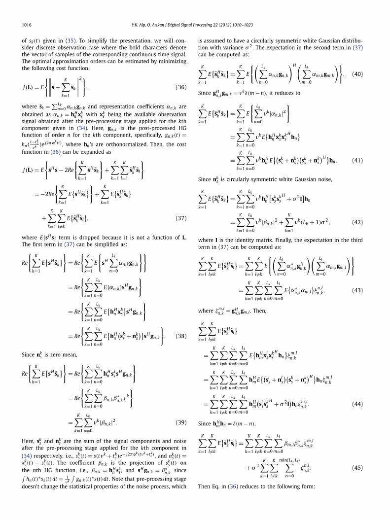
efficients αn , n = 0,1, . . . , L were chosen from a normal distri-bution and the noise samples n(t) were generated from a zeromean Gaussian distribution, whose variance was set according tothe given SNR value. For different representation orders L (rang-ing from 0 to 100), and different SNR values (ranging from −10 dBto 10 dB), we calculated the sample mean and sample standarddeviation of the absolute error between the actual representationorder L and its estimate L, i.e. |L − L|. In Figs. 10(a) and (b), thesetwo statistical measures are plotted as a function of L for differentSNR values. As observed from this plot, even for a complicated sig-nal that is composed of many HGs (e.g. L = 100) and under verylow SNR values (e.g. −10 dB), the average absolute error in expan-sion order estimation is only around 3.5 with standard deviationof 5.5.
Having discussed choosing the expansion orders optimally, thefully automated iterative method for signal component estimationis summarized in Algorithm 1.
When the signal components have overlapping TFSs, decompos-ing the observation signal into its components is a harder problem.
Fig. 10. (a) Ensemble average of the absolute error between actual representationorder L and its estimate L and (b) its standard deviation as a function of L fordifferent SNR values.
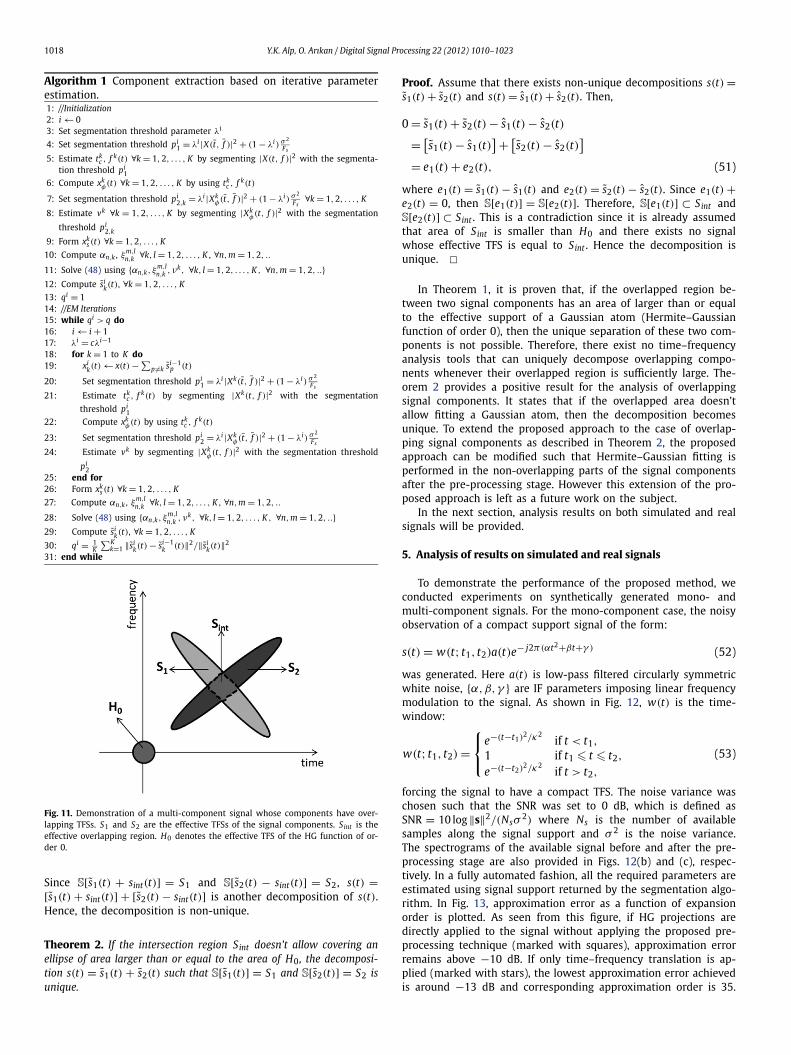
Although the proposed approach is designed for analysis of signalswhose time–frequency components do not have significant over-laps in the time–frequency domain, some insights for the overlap-ping case will be provided. Consider a signal s(t), which have twocomponents with overlapping TFSs s(t) = s1(t) + s2(t), as demon-strated in Fig. 11. In the figure, S1 and S2 denote the effectiveTFS of s1(t) and s2(t), respectively. Sint is the effective support ofthe overlap region. Let S[.] be an operator which returns the ef-fective support of the given signal, i.e., S[sk(t)] = Sk , k = 1,2, andH0 denote the effective support of HG function of order 0, i.e.,S[h0(t)] = H0. The following two theorems explain the uniquenessof the decomposition of s(t) into s1(t) and s2(t) according to thearea of the effective intersection region between the componentsupports.
Theorem 1. If the intersection region Sint allows covering an ellipseof area larger than or equal to the area of H0 , the decompositions(t) = s1(t) + s2(t) such that S[s1(t)] = S1 and S[s1(t)] = S2 is non-unique.
Proof. Since area of Sint is larger than H0, there exist a signalsint(t) with a sufficiently small energy such that S[sint(t)] ⊆ Sint .The decomposition can be rewritten as
s(t) = s1(t) + s2(t)
= s1(t) + s2(t) + sint(t) − sint(t)
= s1(t) + sint(t) + s2(t) − sint(t). (50)
1018 Y.K. Alp, O. Arıkan / Digital Signal Processing 22 (2012) 1010–1023
Algorithm 1 Component extraction based on iterative parameterestimation.1: //Initialization2: i ← 03: Set segmentation threshold parameter λi
4: Set segmentation threshold pi1 = λi |X(t, f )|2 + (1 − λi) σ 2
Fs
5: Estimate tkc , f k(t) ∀k = 1,2, . . . , K by segmenting |X(t, f )|2 with the segmenta-
tion threshold pi1
6: Compute xkφ(t) ∀k = 1,2, . . . , K by using tk
c , f k(t)
7: Set segmentation threshold pi2,k = λi |Xk
φ(t, f )|2 + (1 − λi) σ 2
Fs∀k = 1,2, . . . , K
8: Estimate vk ∀k = 1,2, . . . , K by segmenting |Xkφ(t, f )|2 with the segmentation
threshold pi2,k
9: Form xks (t) ∀k = 1,2, . . . , K
10: Compute αn,k , ξm,ln,k ∀k, l = 1,2, . . . , K , ∀n,m = 1,2, ..
11: Solve (48) using {αn,k, ξm,ln,k , νk, ∀k, l = 1,2, . . . , K , ∀n,m = 1,2, ..}
12: Compute sik(t), ∀k = 1,2, . . . , K
13: qi = 114: //EM Iterations15: while qi > q do16: i ← i + 117: λi = cλi−1
18: for k = 1 to K do19: xi
k(t) ← x(t) − ∑p �=k si−1
p (t)
20: Set segmentation threshold pi1 = λi |Xk(t, f )|2 + (1 − λi) σ 2
Fs
21: Estimate tkc , f k(t) by segmenting |Xk(t, f )|2 with the segmentation
threshold pi1
22: Compute xkφ(t) by using tk
c , f k(t)
23: Set segmentation threshold pi2 = λi |Xk
φ(t, f )|2 + (1 − λi) σ 2
Fs
24: Estimate vk by segmenting |Xkφ(t, f )|2 with the segmentation threshold
pi2
25: end for26: Form xk
s (t) ∀k = 1,2, . . . , K
27: Compute αn,k , ξm,ln,k ∀k, l = 1,2, . . . , K , ∀n,m = 1,2, ..
28: Solve (48) using {αn,k, ξm,ln,k , νk, ∀k, l = 1,2, . . . , K , ∀n,m = 1,2, ..}
29: Compute sik(t), ∀k = 1,2, . . . , K
30: qi = 1K
∑Kk=1 ‖si
k(t) − si−1k (t)‖2/‖si
k(t)‖2
31: end while
Fig. 11. Demonstration of a multi-component signal whose components have over-lapping TFSs. S1 and S2 are the effective TFSs of the signal components. Sint is theeffective overlapping region. H0 denotes the effective TFS of the HG function of or-der 0.
Since S[s1(t) + sint(t)] = S1 and S[s2(t) − sint(t)] = S2, s(t) =[s1(t) + sint(t)] + [s2(t) − sint(t)] is another decomposition of s(t).Hence, the decomposition is non-unique.
Theorem 2. If the intersection region Sint doesn’t allow covering anellipse of area larger than or equal to the area of H0 , the decomposi-tion s(t) = s1(t) + s2(t) such that S[s1(t)] = S1 and S[s2(t)] = S2 isunique.
Proof. Assume that there exists non-unique decompositions s(t) =s1(t) + s2(t) and s(t) = s1(t) + s2(t). Then,
0 = s1(t) + s2(t) − s1(t) − s2(t)
= [s1(t) − s1(t)
] + [s2(t) − s2(t)
]= e1(t) + e2(t), (51)
where e1(t) = s1(t) − s1(t) and e2(t) = s2(t) − s2(t). Since e1(t) +e2(t) = 0, then S[e1(t)] = S[e2(t)]. Therefore, S[e1(t)] ⊂ Sint andS[e2(t)] ⊂ Sint . This is a contradiction since it is already assumedthat area of Sint is smaller than H0 and there exists no signalwhose effective TFS is equal to Sint . Hence the decomposition isunique. �
In Theorem 1, it is proven that, if the overlapped region be-tween two signal components has an area of larger than or equalto the effective support of a Gaussian atom (Hermite–Gaussianfunction of order 0), then the unique separation of these two com-ponents is not possible. Therefore, there exist no time–frequencyanalysis tools that can uniquely decompose overlapping compo-nents whenever their overlapped region is sufficiently large. The-orem 2 provides a positive result for the analysis of overlappingsignal components. It states that if the overlapped area doesn’tallow fitting a Gaussian atom, then the decomposition becomesunique. To extend the proposed approach to the case of overlap-ping signal components as described in Theorem 2, the proposedapproach can be modified such that Hermite–Gaussian fitting isperformed in the non-overlapping parts of the signal componentsafter the pre-processing stage. However this extension of the pro-posed approach is left as a future work on the subject.
In the next section, analysis results on both simulated and realsignals will be provided.
5. Analysis of results on simulated and real signals
To demonstrate the performance of the proposed method, weconducted experiments on synthetically generated mono- andmulti-component signals. For the mono-component case, the noisyobservation of a compact support signal of the form:
s(t) = w(t; t1, t2)a(t)e− j2π(αt2+βt+γ ) (52)
was generated. Here a(t) is low-pass filtered circularly symmetricwhite noise, {α,β,γ } are IF parameters imposing linear frequencymodulation to the signal. As shown in Fig. 12, w(t) is the time-window:
w(t; t1, t2) =⎧⎨⎩
e−(t−t1)2/κ2if t < t1,
1 if t1 � t � t2,
e−(t−t2)2/κ2if t > t2,
(53)
forcing the signal to have a compact TFS. The noise variance waschosen such that the SNR was set to 0 dB, which is defined asSNR = 10 log ‖s‖2/(Nsσ
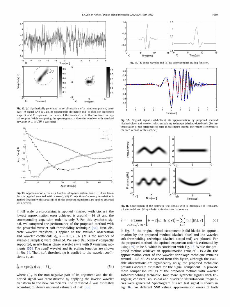
2) where Ns is the number of availablesamples along the signal support and σ 2 is the noise variance.The spectrograms of the available signal before and after the pre-processing stage are also provided in Figs. 12(b) and (c), respec-tively. In a fully automated fashion, all the required parameters areestimated using signal support returned by the segmentation algo-rithm. In Fig. 13, approximation error as a function of expansionorder is plotted. As seen from this figure, if HG projections aredirectly applied to the signal without applying the proposed pre-processing technique (marked with squares), approximation errorremains above −10 dB. If only time–frequency translation is ap-plied (marked with stars), the lowest approximation error achievedis around −13 dB and corresponding approximation order is 35.
Y.K. Alp, O. Arıkan / Digital Signal Processing 22 (2012) 1010–1023 1019
Fig. 12. (a) Synthetically generated noisy observation of a mono-component, com-pact TFS signal. SNR is 0 dB. Its spectrogram (b) before and (c) after pre-processingstage. R and R ′ represent the radius of the smallest circle that encloses the sig-nal support. While computing the spectrograms, a Gaussian window with standarddeviation σ = 1/
√2π s was used.
Fig. 13. Approximation error as a function of approximation order: (i) if no trans-form is applied (marked with squares); (ii) if only time–frequency translation isapplied (marked with stars); (iii) if all the proposed transforms are applied (markedwith circles).
If full scale pre-processing is applied (marked with circles), thelowest approximation error achieved is around −16 dB and thecorresponding expansion order is only 7. For this synthetic sig-nal, we compared the performance of the proposed method withthe powerful wavelet soft-thresholding technique [34]. First, dis-crete wavelet transform is applied to the available observationand wavelet coefficients ξk , k = 0,1,2.., N (N is the number ofavailable samples) were obtained. We used Daubechies’ compactlysupported, nearly linear phase wavelet sym8 with 9 vanishing mo-ments [35]. The sym8 wavelet and its scaling function are shownin Fig. 14. Then, soft thresholding is applied to the wavelet coeffi-cients ξk as:
ξk = sgn(ξk)(|ξk| − ε
)+, (54)
where (.)+ is the non-negative part of its argument and the de-noised signal was reconstructed by applying the inverse wavelettransform to the new coefficients. The threshold ε was estimatedaccording to Stein’s unbiased estimate of risk [36]:
Fig. 14. (a) Sym8 wavelet and (b) its corresponding scaling function.
Fig. 15. Original signal (solid-black), its approximation by proposed method(dashed-blue) and wavelet soft-thresholding technique (dashed-doted-red). (For in-terpretation of the references to color in this figure legend, the reader is referred tothe web version of this article.)
Fig. 16. Spectrogram of the synthetic test signals with (a) triangular, (b) constant,(c) sinusoidal and (d) quadratic instantaneous frequencies.
ε = arg min0�ε�
√2 log N
[N − 2
{k: |ξk � ε|} +
N∑k=1
min(|ξk|, ε
)]. (55)
In Fig. 15, the original signal component (solid-black), its approx-imation by the proposed method (dashed-blue) and the waveletsoft-thresholding technique (dashed-dotted-red) are plotted. Forthe proposed method, the optimal expansion order is estimated byusing (49) to be 5, which is consistent with Fig. 13. While the pro-posed method achieves an approximation error of −15.2 dB, theapproximation error of the wavelet shrinkage technique remainsaround −6.8 dB. As observed from this figure, although the avail-able observations are significantly noisy, the proposed techniqueprovides accurate estimates for the signal component. To providemore comparison results of the proposed method with waveletsoft-thresholding technique, four more synthetic signals with tri-angular, constant, sinusoidal and quadratic instantaneous frequen-cies were generated. Spectrogram of each test signal is shown inFig. 16. For different SNR values, approximation errors of both
1020 Y.K. Alp, O. Arıkan / Digital Signal Processing 22 (2012) 1010–1023
Table 1Approximation errors of the proposed method (Prop. Meth.) and wavelet soft-thresholding (W.S. Thres.) for the test signals with triangular (Trian.), constant(Cons.), sinusoidal (Sin.) and quadratic (Quad.) instantaneous frequencies shown inFig. 16, for different SNR values.
Trian. Cons. Sin. Quad.
SNR = 0 dB Prop. Meth. −13.6 −14.9 −14.6 −12.8SNR = 0 dB W.S. Thres. −9.1 −10.5 −7.9 −9.8SNR = 5 dB Prop. Meth. −17.6 −19.4 −15.6 −15.8SNR = 5 dB W.S. Thres. −9.8 −12.8 −9 −11.6
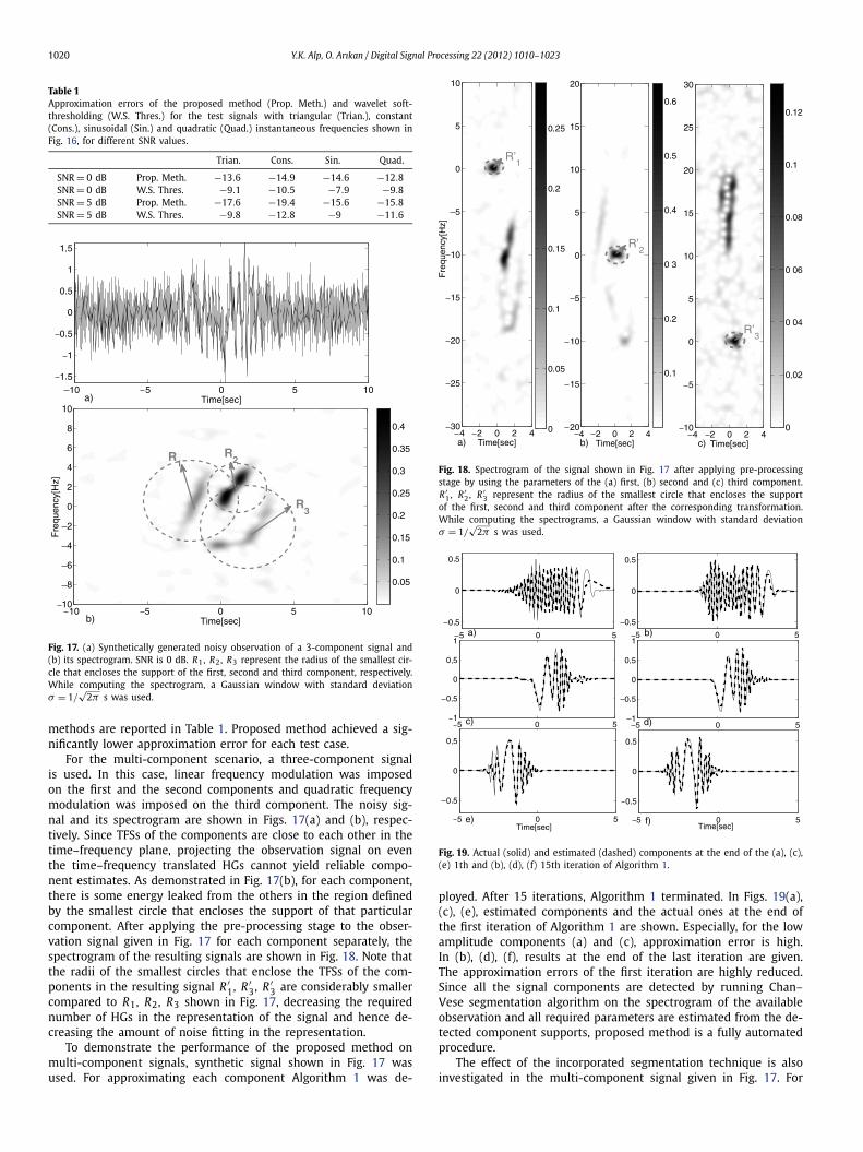
Fig. 17. (a) Synthetically generated noisy observation of a 3-component signal and(b) its spectrogram. SNR is 0 dB. R1, R2, R3 represent the radius of the smallest cir-cle that encloses the support of the first, second and third component, respectively.While computing the spectrogram, a Gaussian window with standard deviationσ = 1/
√2π s was used.
methods are reported in Table 1. Proposed method achieved a sig-nificantly lower approximation error for each test case.
For the multi-component scenario, a three-component signalis used. In this case, linear frequency modulation was imposedon the first and the second components and quadratic frequencymodulation was imposed on the third component. The noisy sig-nal and its spectrogram are shown in Figs. 17(a) and (b), respec-tively. Since TFSs of the components are close to each other in thetime–frequency plane, projecting the observation signal on eventhe time–frequency translated HGs cannot yield reliable compo-nent estimates. As demonstrated in Fig. 17(b), for each component,there is some energy leaked from the others in the region definedby the smallest circle that encloses the support of that particularcomponent. After applying the pre-processing stage to the obser-vation signal given in Fig. 17 for each component separately, thespectrogram of the resulting signals are shown in Fig. 18. Note thatthe radii of the smallest circles that enclose the TFSs of the com-ponents in the resulting signal R ′
1, R ′3, R ′
3 are considerably smallercompared to R1, R2, R3 shown in Fig. 17, decreasing the requirednumber of HGs in the representation of the signal and hence de-creasing the amount of noise fitting in the representation.
To demonstrate the performance of the proposed method onmulti-component signals, synthetic signal shown in Fig. 17 wasused. For approximating each component Algorithm 1 was de-
Fig. 18. Spectrogram of the signal shown in Fig. 17 after applying pre-processingstage by using the parameters of the (a) first, (b) second and (c) third component.R ′
1, R ′2, R ′
3 represent the radius of the smallest circle that encloses the supportof the first, second and third component after the corresponding transformation.While computing the spectrograms, a Gaussian window with standard deviationσ = 1/
√2π s was used.
Fig. 19. Actual (solid) and estimated (dashed) components at the end of the (a), (c),(e) 1th and (b), (d), (f) 15th iteration of Algorithm 1.
ployed. After 15 iterations, Algorithm 1 terminated. In Figs. 19(a),(c), (e), estimated components and the actual ones at the end ofthe first iteration of Algorithm 1 are shown. Especially, for the lowamplitude components (a) and (c), approximation error is high.In (b), (d), (f), results at the end of the last iteration are given.The approximation errors of the first iteration are highly reduced.Since all the signal components are detected by running Chan–Vese segmentation algorithm on the spectrogram of the availableobservation and all required parameters are estimated from the de-tected component supports, proposed method is a fully automatedprocedure.
The effect of the incorporated segmentation technique is alsoinvestigated in the multi-component signal given in Fig. 17. For
Y.K. Alp, O. Arıkan / Digital Signal Processing 22 (2012) 1010–1023 1021
Table 2Normalized approximation error and energy difference for each component esti-mated by utilizing Chan–Vese and Watershed segmentation techniques in the pro-posed method.
Norm. App. Err/Comp. p1(t) p2(t) p3(t)
ecv −14.7 −16.1 −14.3ew −14.3 −15.6 −14.8ed 0.17 0.25 0.21
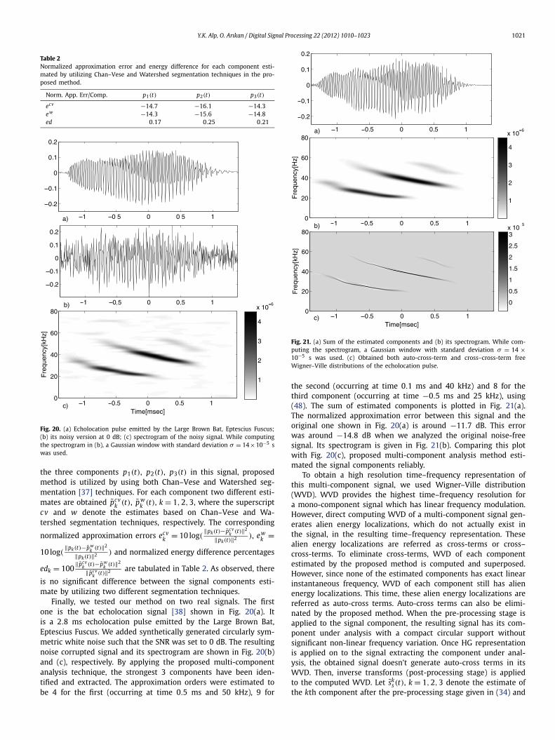
Fig. 20. (a) Echolocation pulse emitted by the Large Brown Bat, Eptescius Fuscus;(b) its noisy version at 0 dB; (c) spectrogram of the noisy signal. While computingthe spectrogram in (b), a Gaussian window with standard deviation σ = 14×10−5 swas used.
the three components p1(t), p2(t), p3(t) in this signal, proposedmethod is utilized by using both Chan–Vese and Watershed seg-mentation [37] techniques. For each component two different esti-mates are obtained pcv
k (t), pwk (t), k = 1,2,3, where the superscript
cv and w denote the estimates based on Chan–Vese and Wa-tershed segmentation techniques, respectively. The corresponding
normalized approximation errors ecvk = 10 log(
‖pk(t)−pcvk (t)‖2
‖pk(t)‖2 ), ewk =
10 log(‖pk(t)−pw
k (t)‖2
‖pk(t)‖2 ) and normalized energy difference percentages
edk = 100‖pcv
k (t)−pwk (t)‖2
‖pcvk (t)‖2 are tabulated in Table 2. As observed, there
is no significant difference between the signal components esti-mate by utilizing two different segmentation techniques.
Finally, we tested our method on two real signals. The firstone is the bat echolocation signal [38] shown in Fig. 20(a). Itis a 2.8 ms echolocation pulse emitted by the Large Brown Bat,Eptescius Fuscus. We added synthetically generated circularly sym-metric white noise such that the SNR was set to 0 dB. The resultingnoise corrupted signal and its spectrogram are shown in Fig. 20(b)and (c), respectively. By applying the proposed multi-componentanalysis technique, the strongest 3 components have been iden-tified and extracted. The approximation orders were estimated tobe 4 for the first (occurring at time 0.5 ms and 50 kHz), 9 for
Fig. 21. (a) Sum of the estimated components and (b) its spectrogram. While com-puting the spectrogram, a Gaussian window with standard deviation σ = 14 ×10−5 s was used. (c) Obtained both auto-cross-term and cross–cross-term freeWigner–Ville distributions of the echolocation pulse.
the second (occurring at time 0.1 ms and 40 kHz) and 8 for thethird component (occurring at time −0.5 ms and 25 kHz), using(48). The sum of estimated components is plotted in Fig. 21(a).The normalized approximation error between this signal and theoriginal one shown in Fig. 20(a) is around −11.7 dB. This errorwas around −14.8 dB when we analyzed the original noise-freesignal. Its spectrogram is given in Fig. 21(b). Comparing this plotwith Fig. 20(c), proposed multi-component analysis method esti-mated the signal components reliably.
To obtain a high resolution time–frequency representation ofthis multi-component signal, we used Wigner–Ville distribution(WVD). WVD provides the highest time–frequency resolution fora mono-component signal which has linear frequency modulation.However, direct computing WVD of a multi-component signal gen-erates alien energy localizations, which do not actually exist inthe signal, in the resulting time–frequency representation. Thesealien energy localizations are referred as cross-terms or cross–cross-terms. To eliminate cross-terms, WVD of each componentestimated by the proposed method is computed and superposed.However, since none of the estimated components has exact linearinstantaneous frequency, WVD of each component still has alienenergy localizations. This time, these alien energy localizations arereferred as auto-cross terms. Auto-cross terms can also be elimi-nated by the proposed method. When the pre-processing stage isapplied to the signal component, the resulting signal has its com-ponent under analysis with a compact circular support withoutsignificant non-linear frequency variation. Once HG representationis applied on to the signal extracting the component under anal-ysis, the obtained signal doesn’t generate auto-cross terms in itsWVD. Then, inverse transforms (post-processing stage) is appliedto the computed WVD. Let sk
s (t), k = 1,2,3 denote the estimate ofthe kth component after the pre-processing stage given in (34) and
1022 Y.K. Alp, O. Arıkan / Digital Signal Processing 22 (2012) 1010–1023
Fig. 22. (a) EEG recording and (b) its spectrogram. While computing the spectro-gram, a Gaussian window with standard deviation σ = 0.1/
√2π s was used.
Fig. 23. Estimated signal components (a)–(c) from the EEG recording shown inFig. 22.
WVks (t, f ) denote its WVD. The auto-cross-term-free WVD of sk(t)
is given by:
WVk(t, f ) = 1
vkWVk
s
(t − tk
c
vk, vk( f − f k(t)
)), (56)
where {tkc , f k(t), vk}, k = 1,2,3 are the transform parameters. The
sum WV(t, f ) = WV1(t, f ) + WV2(t, f ) + WV3(t, f ) is both auto-cross term and cross–cross-term free WVD of the bath echoloca-tion pulse and shown in Fig. 21(c).
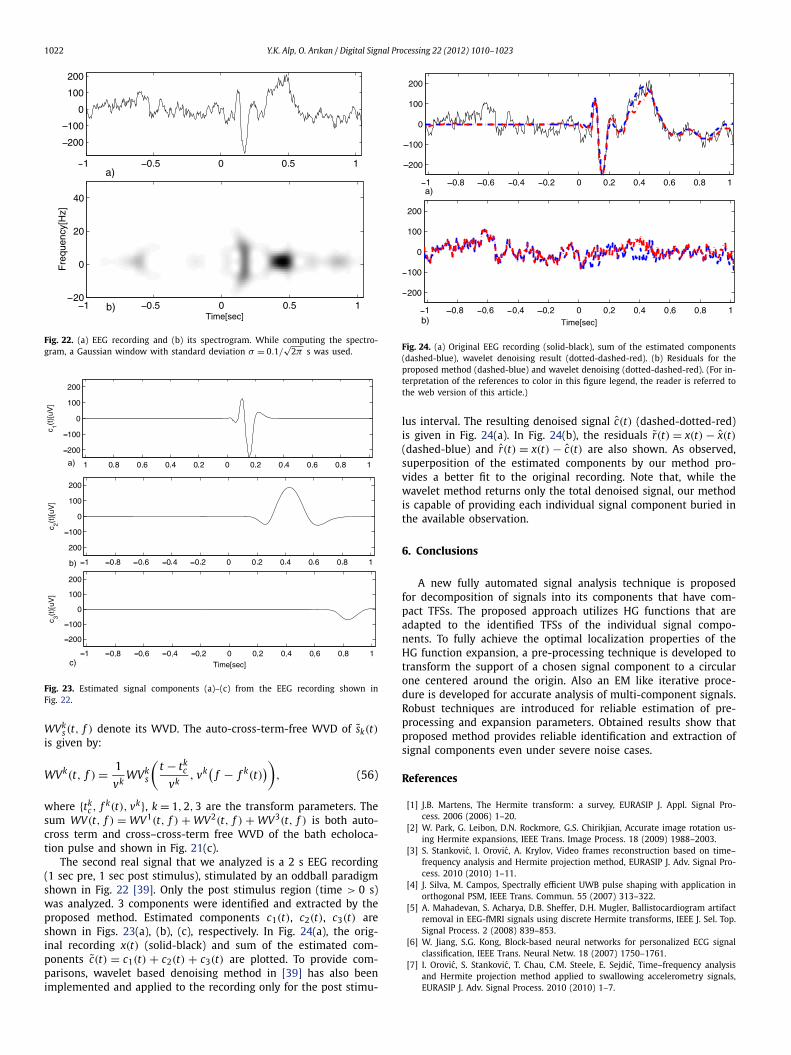
The second real signal that we analyzed is a 2 s EEG recording(1 sec pre, 1 sec post stimulus), stimulated by an oddball paradigmshown in Fig. 22 [39]. Only the post stimulus region (time > 0 s)was analyzed. 3 components were identified and extracted by theproposed method. Estimated components c1(t), c2(t), c3(t) areshown in Figs. 23(a), (b), (c), respectively. In Fig. 24(a), the orig-inal recording x(t) (solid-black) and sum of the estimated com-ponents c(t) = c1(t) + c2(t) + c3(t) are plotted. To provide com-parisons, wavelet based denoising method in [39] has also beenimplemented and applied to the recording only for the post stimu-
Fig. 24. (a) Original EEG recording (solid-black), sum of the estimated components(dashed-blue), wavelet denoising result (dotted-dashed-red). (b) Residuals for theproposed method (dashed-blue) and wavelet denoising (dotted-dashed-red). (For in-terpretation of the references to color in this figure legend, the reader is referred tothe web version of this article.)
lus interval. The resulting denoised signal c(t) (dashed-dotted-red)is given in Fig. 24(a). In Fig. 24(b), the residuals r(t) = x(t) − x(t)(dashed-blue) and r(t) = x(t) − c(t) are also shown. As observed,superposition of the estimated components by our method pro-vides a better fit to the original recording. Note that, while thewavelet method returns only the total denoised signal, our methodis capable of providing each individual signal component buried inthe available observation.
6. Conclusions
A new fully automated signal analysis technique is proposedfor decomposition of signals into its components that have com-pact TFSs. The proposed approach utilizes HG functions that areadapted to the identified TFSs of the individual signal compo-nents. To fully achieve the optimal localization properties of theHG function expansion, a pre-processing technique is developed totransform the support of a chosen signal component to a circularone centered around the origin. Also an EM like iterative proce-dure is developed for accurate analysis of multi-component signals.Robust techniques are introduced for reliable estimation of pre-processing and expansion parameters. Obtained results show thatproposed method provides reliable identification and extraction ofsignal components even under severe noise cases.
References
[1] J.B. Martens, The Hermite transform: a survey, EURASIP J. Appl. Signal Pro-cess. 2006 (2006) 1–20.
[2] W. Park, G. Leibon, D.N. Rockmore, G.S. Chirikjian, Accurate image rotation us-ing Hermite expansions, IEEE Trans. Image Process. 18 (2009) 1988–2003.
[3] S. Stankovic, I. Orovic, A. Krylov, Video frames reconstruction based on time–frequency analysis and Hermite projection method, EURASIP J. Adv. Signal Pro-cess. 2010 (2010) 1–11.
[4] J. Silva, M. Campos, Spectrally efficient UWB pulse shaping with application inorthogonal PSM, IEEE Trans. Commun. 55 (2007) 313–322.
[5] A. Mahadevan, S. Acharya, D.B. Sheffer, D.H. Mugler, Ballistocardiogram artifactremoval in EEG-fMRI signals using discrete Hermite transforms, IEEE J. Sel. Top.Signal Process. 2 (2008) 839–853.
[6] W. Jiang, S.G. Kong, Block-based neural networks for personalized ECG signalclassification, IEEE Trans. Neural Netw. 18 (2007) 1750–1761.
[7] I. Orovic, S. Stankovic, T. Chau, C.M. Steele, E. Sejdic, Time–frequency analysisand Hermite projection method applied to swallowing accelerometry signals,EURASIP J. Adv. Signal Process. 2010 (2010) 1–7.
Y.K. Alp, O. Arıkan / Digital Signal Processing 22 (2012) 1010–1023 1023
[8] M.M. Rao, T.K. Sarkar, T. Anjali, R.S. Adve, Simultaneous extrapolation intime and frequency domains using Hermite expansions, IEEE Trans. AntennasPropag. 47 (1999) 1108–1115.
[9] P.L. Carro, J.D. Mingo, Ultrawide-band antenna distortion characterization usingHermite–Gauss signal subspaces, IEEE Antennas Wirel. Propag. Lett. 7 (2008)267–270.
[10] I. Orovic, S. Stankovic, T. Thayaparan, L. Stankovic, Multiwindow s-method forinstantaneous frequency estimation and its application in radar signal analysis,IET Signal Process. 4 (2010) 363–370.
[11] J. Xiao, P. Flandrin, Multitaper time–frequency reassignment for nonstationaryspectrum estimation and chirp enhancement, IEEE Trans. Signal Process. 55(2007) 2851–2860.
[12] M. Bayram, R.G. Baraniuk, Multiple Window Time-Varying Spectrum Estima-tion in Nonlinear and Nonstationary Signal Processing, Cambrigde Univ. Press,Cambridge, 2000.
[13] F. Cakrak, P.J. Loughlin, Multiple window time-varying spectral analysis, IEEETrans. Signal Process. 49 (2001) 448–453.
[14] V.C. Chen, H. Ling, Joint time–frequency analysis for radar signal and imageprocessing, IEEE Signal Process. Mag. 16 (1999) 81–93.
[15] M. Ning, D. Vray, Bottom backscattering coefficient estimation from widebandchirp sonar echoes by chirp adapted time–frequency representation, in: Pro-ceedings of the 1998 IEEE International Conference on Acoustics, Speech andSignal Processing, Seattle, USA, pp. 2461–2464.
[16] R.G. Baraniuk, M. Coates, P. Steeghs, Hybrid linear/quadratic time–frequency at-tributes, IEEE Trans. Signal Process. 49 (2001) 760–766.
[17] B. Boashash, P. O’shea, Time–frequency analysis applied to signaturing of un-derwater acoustic signals, in: Proceedings of the 1988 IEEE International Con-ference on Acoustics, Speech and Signal Processing, New York, USA, pp. 2817–2820.
[18] O. Yilmaz, S. Rickard, Blind separation of speech mixtures via time–frequencymasking, IEEE Trans. Signal Process. 52 (2004) 1830–1847.
[19] A.K. Ozdemir, S. Karakas, E.D. Cakmak, D.I. Tufekci, O. Arikan, Time–frequencycomponent analyser and its application to brain oscillatory activity, J. Neurosci.Methods 145 (2005) 107–125.
[20] A.K. Ozdemir, Time–frequency component analyzer, Ph.D. thesis, Bilkent Uni-versity, Ankara, Turkey, 2003.
[21] L. Durak, O. Arikan, Short-time Fourier transform: two fundamental propertiesand an optimal implementation, IEEE Trans. Signal Process. 51 (2003) 1231–1242.
[22] I. Daubechies, The wavelet transform, time–frequency localization and signalanalysis, IEEE Trans. Inform. Theory 36 (1990) 961–1005.
[23] S. Mann, S. Haykin, The chirplet transform: physical considerations, IEEE Trans.Signal Process. 43 (1995) 2745–2761.
[24] N. Nebedev, Special Functions and Their Applications, Dover, New York, 1972.[25] P. Flandrin, Maximum signal energy concentration in a time–frequency domain,
in: Proceedings of the 1988 IEEE International Conference on Acoustics, Speechand Signal Processing, New York, USA, pp. 2176–2179.
[26] I. Daubechies, Time–frequency localization operators: a geometric phase spaceapproach, IEEE Trans. Inform. Theory 34 (1988) 605–612.
[27] F. Hlawatsch, Time–Frequency Analysis and Synthesis of Linear Signal Spaces,Kluwer, 1998.
[28] L.R. Conte, R. Merletti, G.V. Sandri, Hermite expansions of compact supportwaveforms: applications to myelectric signals, IEEE Trans. Biomed. Eng. 41(1994) 1147–1159.
[29] M. Abramowitz, I. Stegun, Handbook of Mathematical Functions, Dover, NewYork, 1965.
[30] G. Cincotti, F. Gori, M. Santarsiero, Generalized self Fourier functions, J. Phys.,A, Math. Gen. 25 (1992) 1191–1194.
[31] H. Ozaktas, B. Barshan, D. Mendlovic, L. Onural, Convolution, filtering and mul-tiplexing in fractional Fourier domains and relations to chirp and wavelettransforms, J. Opt. Soc. Amer. A 11 (1994) 547–559.
[32] L. Cohen, Time–Frequency Analysis, Prentice Hall PTR, Englewood Cliffs, NJ,1995.
[33] T.F. Chan, L.A. Vese, Active contours without edges, IEEE Trans. Image Pro-cess. 10 (2001) 266–277.
[34] D.L. Donoho, De-noising by soft thresholding, IEEE Trans. Inform. Theory 41(1995) 613–627.
[35] I. Daubechies, Ten Lectures on Wavelets, SIAM, 1992.[36] D.L. Donoho, M. Johnstone, Adapting to unknown smoothness via wavelet
shrinkage, J. Amer. Statist. Assoc. 90 (1995) 1200–1224.[37] J.K.L. Shafarenko, M. Petrou, Automatic watershed segmentation of randomly
textured color images, IEEE Trans. Image Process. 6 (1997) 1530–1544.[38] Bat echolocation signal, http://dsp.rice.edu/software/bat-echolocation-chirp,
2009.[39] R. Quiroga, Obtaining single stimulus evoked potentials with wavelet denoising,
Physica D 145 (2000) 278–292.
Yasar Kemal Alp was born in Konya, Turkey, in 1985. He received hisB.Sc. degree in electrical and electronics engineering from Bilkent Univer-sity, Ankara, Turkey. He worked as a Research Scientist in SchlumbergerCambridge Research between June–August 2009 and July–September 2010.He is currently pursuing his Ph.D. in Department of Electrical and Elec-tronics Engineering, Bilkent University. His research interests are time–frequency signals analysis, inverse problems and their applications toradar signal processing.
Orhan Arıkan was born in 1964 in Manisa, Turkey. He received theB.Sc. degree in electrical and electronics engineering from the MiddleEast Technical University, Ankara, Turkey in 1986 and both the M.S. andPh.D. degrees in electrical and computer engineering from the Universityof Illinois, Urbana-Champaign, in 1988 and 1990, respectively. Followinghis graduate studies, he worked for three years as a Research Scientistat Schlumberger – Doll Research, Ridgefield, CT. He joined Bilkent Uni-versity in 1993, where he is presently Professor of Electrical Engineeringsince 2006 and chair of the Electrical Engineering Department since 2011.His current research interests are in statistical signal processing, time–frequency analysis, and array signal processing.


![Face Recognition using Spherical Waveletself/.misc/phd_project_lessig.pdf · 2008. 1. 10. · for face recognition; and Wu et al. [55] employed horizontal profiles. Gaussian-Hermite](https://img.pdfslide.us/doc/110x75/6027f41b0ebb7351336aef76/face-recognition-using-spherical-elfmiscphdprojectlessigpdf-2008-1-10.jpg)


![arXiv:1407.0730v4 [physics.optics] 18 Oct 2015 · Key words and phrases. Paraxial wave equation, Green’s function, generalized Fresnel integrals, Airy-Hermite-Gaussian beams, Hermite-Gaussian](https://img.pdfslide.us/doc/110x75/607256db68e9bf2b096e18e3/arxiv14070730v4-18-oct-2015-key-words-and-phrases-paraxial-wave-equation.jpg)