Time zones matter: The impact of distance

and timezones on services trade ∗

Elisabeth ChristenUniversitat Innsbruck, and Johannes Kepler Universitat Linz

August 1, 2011

Abstract

Using distance and time zone differences as a measure for coordinationcosts between service suppliers and consumers, we employ a Hausman-Taylor model for services trade through foreign affiliates. Given the needfor proximity in the provision of services, factors like distance place ahigher cost burden on the provision of services. In addition, differencesin time zones add significantly to the cost of doing business abroad. Bydecomposing the impact of distance into a longitudinal and latitudinalcomponent and accounting for differences in time zones, we can identifyin detail the factors driving the impact of increasing coordination costs onthe delivery of services through foreign affiliates. Working with a bilateralU.S. data set on foreign affiliate sales in services we examine the impactof time zone differences and East-West and North-South distance on U.S.outward affiliate sales. We find that both distance as well as time zone dif-ferences have a consistent positive and significant effect on foreign affiliatesales. By decomposing the effect of distance our results show that increas-ing East-West or North-South distance by 100 kilometers raises affiliatessales by 2%. Finally, focusing on time zone differences our findings suggestthat affiliate sales increase the more time zones we have to overcome.

Keywords: Foreign Affiliates Trade, International Trade in Services, Co-ordination Costs, Time zonesJEL codes: F14, F21, F23, L80

∗Address for correspondence: Elisabeth Christen, Leopold Franzens University of Inns-bruck, Department of Economics & Statistics, Universitatsstr. 15, 6020 Innsbruck, Austria.email: elisabeth.christen@uibk.ac.at

1 Introduction

Given that services are a flow and not a stock, direct proximity and interaction

between supplier and consumer are more important for trade in services than for

trade in goods. From a historical viewpoint, this has hampered growth in inter-

national services trade relative to commodities trade. However, due to technical

change, the proximity burden has progressively weakened in recent decades for

some (but not all) service activities (Christen and Francois, 2010). This has

evoked a dramatic growth in services trade and foreign investment and has led

to a nascent empirical and theoretical literature on trade in services (Francois

and Hoekman, 2010). However, the non-storable nature of services may still

imply a double coincidence in both time and space of the proximity between

the provider and the consumer (Kikuchi and Marjit, 2010). This means that

factors like distance place an additional cost burden on some aspects of service

provision. Additionally, time zone differences add significantly to the cost of do-

ing business abroad. In this paper, we disentangle the impact of distance from

longitudinal and latitudinal distance as well as time zone differences on services

trade through foreign affiliates using a panel of U.S. affiliate sales. Our data

on affiliate sales allows more sector detail than found in the recent literature,

which relies instead on FDI as a proxy for affiliate sales. We show that time

zone differences as well as latitudinal and longitudinal distance in particular are

major drivers for U.S. outward affiliates sales.

Questions raised in the recent literature on services trade and investment are

closely related to the large body of empirical evidence regarding determinants

of multinational activity with respect to goods production and trade. But the

data issues are even more severe for services investment than for goods, placing

even more constraints on the scope for empirical analysis of services trade and

FDI linkages. Indeed, because of data issues the recent literature along these

lines uses FDI flows or stocks as a proxy for affiliate sales. For example, Grun-

feld and Moxnes (2003) explore the determinants of services trade and foreign

affiliate sales using FDI stocks as a proxy for foreign affiliate sales in a gravity

model. They find that trade barriers and distance have a strong negative im-

pact on exports and FDI, while GDP and similar income levels have a significant

positive impact. Kolstad and Villanger (2008) study the determinants of service

FDI with panel analysis for the whole service sector and a small number of sub-

sectors. They conclude that FDI in services tends to be more market seeking

and find strong correlation between manufacturing FDI and FDI in producer

services as well as an important impact of institutional quality and democracy

2

on services FDI. Furthermore, a recent study by Christen and Francois (2010)

suggests that the overall response of individual service firms aggregated by in-

dustries to distance leads to a striking difference in the impact of distance on

the mix of affiliate sales and direct cross-border exports when comparing goods

and services. The authors’ findings show that at the industry level, the impor-

tance of proximity between supplier and consumer appears empirically robust

in explaining increased affiliate activity relative to cross-border sales with in-

creased distance. They show that multinational activity in services increases

relative to direct exports the further away are host countries, the lower are in-

vestment barriers and the higher is manufacturing FDI, while common language

familiarities and bigger markets foster affiliate activity additionally.

To summarize, recent literature on trade in services highlighted the role of

distance as a cost burden and further transactions costs that may affect the

cost of doing business. In particular, empirical literature based on the gravity

models of bilateral trade distinguished between two sets of variables to account

for transactions costs. The first group of variables is based on geographical

characteristics across countries and country pairs, such as distance, contiguity,

or whether one or both countries in the pair are landlocked and mainly cap-

ture costs directly linked to transportation costs. The second group comprises

variables related to cultural and historical ties between countries, such as com-

mon language, past colonial links and similar cultural heritages and take into

account further transaction costs that may affect the cost of doing business

abroad. However, none of these variables precisely capture transactions costs

due to the need of real time interaction between providers and buyers like it is

the case for trade in services. Of course, recent developments in telecommunica-

tion, like e-mail and teleconference communication, contributed to reduce costs

of transaction and facilitated (real time) communication. Since those technical

improvements are in a broader sense substitutable with face-to-face interaction

North-South distances can be overcome more easily. However, differences in

time zones can matter and can not be neglected in terms of transaction costs.

Time zone differences are present in real time communication as well as in travel

and increasing East-West distance can have major negative impacts on both.

Regarding real time communication, time zone differences between two coun-

tries impedes communication and may lead in the extreme case to no overlap

in business working hours. With respect to traveling, East-West distance is

more severe since a jet lag may affect the productivity of business travelers.

Interactions between provider and user in real time are especially relevant for

information intensive services that require a high degree of interaction in real

3

time. Frequent real time communication is in particular important between

headquarters and their foreign affiliates, thus looking at foreign affiliate sales

seems to be a good approach to us to examine the effects of time zone differ-

ences, and in particular differences in longitudinal and latitudinal distance.

So far little attention has be paid to the impact of time zones on economic

outcomes. There exist few papers that address the determinants of bilateral

equity flows and returns. Kamstra et al. (2000) study the effect of changes due

to daylight saving time on equity returns and their results show that returns are

significantly lower after daylight saving time changes. Portes and Rey (2005)

examine the impact of bilateral distance on bilateral equity flows and the au-

thors find a significantly negative effect of distance which can be interpreted in

terms of informational cost between local and foreign investors. Furthermore

the results support that overlapping stock market trading hours, a variable that

accounts in some sense for time zone differences, have a significant positive ef-

fect on equity flows. Given these findings increased coordination costs due to

time zone differences should have an important impact on foreign affiliate sales.

In a similar paper Loungani et al. (2002) extend the work by Portes and Rey

(2005) to the case of bilateral FDI flows. Their results show that trade as well

as investment flows rises as ”transactional distance” is reduced. Hattari and

Rajan (2008) examine the role of distance and time zone differences on FDI

flows to developing Asia using bilateral FDI flows over the period 1990 to 2005.

Their results suggest that physical distance is partly captured by the effect of

time zone differences and that time zone differences appear to hamper FDI flows.

In a related paper, Stein and Daude (2007) estimate the effects of time zone

differences on bilateral stocks of foreign direct investment (FDI) in a cross-

section analysis. They use OECD data for 17 OECD source and 58 host coun-

tries over a period from 1997 to 1999 and show that longitudinal distance in the

form of time zone differences impose important transaction costs between par-

ties. Besides using time zone differences to account for transaction costs, they

authors also decompose the distance between a country pair into a longitudinal

and latitudinal component. Their findings show that differences in time zones

have a significantly negative impact on the location of FDI. Moreover, both

components of distance (North-South and East-West) are significant and have

a negative impact on bilateral FDI stocks. However, the impact of longitudinal

distance is significantly larger than the latitudinal measure. In an extension the

authors study the importance of time zone differences as a determinant of bilat-

4

eral trade and their findings suggest that differences in time zones also matter

for trade, but the impact is much smaller than compared to the one found for

FDI. For robustness checks the authors also apply alternative measures of time

zone differences, such as minimum time zone differences to account for countries

with multiple time zones and overlapping business hours, similar to the variable

- overlap in trading hours - used by Portes and Rey (2005).

We proceed in this paper as follows. In Section 2, we describe the data

set and the explain in detail the decomposition of distance into a longitudinal

and latitudinal component. The subsequent Section 3 discusses the empirical

strategy and presents the results. We offer a brief summary and concluding

remarks in Section 4.

2 Data and the decomposition of distance

In order to examine the effects of time zone differences on the location of foreign

direct investment, we use outward affiliates sales data from the United States.

These detailed data on U.S. direct investment abroad is drawn from the Bench-

mark Surveys conducted by the Bureau of Economic Analysis (BEA) which are

published every five years. The benchmark surveys offer the most comprehen-

sive dataset with respect to firms covered and disaggregation of the data. U.S.

direct investment abroad comprises all foreign business enterprises which are

owned at least 10 percent, directly or indirectly, by a U.S. investor. The data

for foreign affiliates are disaggregated by country and industry of the affiliate

or by industry of the U.S. parent. Besides the advantageous structure of the

information gathered on the affiliates abroad, the surveys additionally collect

data on the financial structure of the U.S. parent and their foreign affiliates

as well as on balance of payments transactions between the two parties. This

allows for a very precise analysis of sales of services by majority-owned foreign

affiliates.1 For our purposes we make use of the information gathered on sales

of services by majority-owned foreign affiliates to foreigners in the non-bank

field, disaggregated by country and industry of the affiliate. The classification

by country of the affiliate defines the country in which the affiliate’s physical

1In this surveys, data on foreign affiliates and their U.S.parents are presented for five groups- all affiliates and any combinations between bank and non-bank affiliates and parents as well asdifferences in ownership. In this paper, we entirely focus on majority-owned nonbank affiliatesof nonbank U.S. parents. A majority-owned foreign affiliate (MOFA) is a foreign affiliatein which the combined direct and indirect ownership interest of all U.S. parents exceeds 50percent. Data for MOFAs rather than for all foreign affiliates are relevant in order to examinethe foreign investments over which U.S. parents exert unambiguous control (U.S. Bureau ofEconomic Analysis, 2008).

5

assets are located or in which its primary activity is carried out. The industry

classification based on NAICS (North American Industry Classification System)

was assigned on the basis of the sector accounting for the largest percentage of

sales. Individual service sectors are typically characterized by a handful of large

firms representing a relatively large share of the market. Thus, data points are

frequently suppressed in published data because they represent the data of a

single firm, and as such the data reveal confidential business information. More-

over BEA also does not report small values of affiliate sales, in detail non-zero

values smaller than half a million U.S. Dollars.

Our dataset comprises information for 61 partner countries for five different

service sectors - wholesale trade, information services, financial and insurance

services, professional, scientific and technical services as well as the combined

sector other industries. In total we gather information from four benchmark

surveys covering the years 1989, 1994, 1999 and 2004. Over the time horizon

affiliate sales in all service sectors across partner countries increased steadily,

whereby the highest growth was in other industries followed by financial and

insurance service and professional, scientific and technical services.

To identify the determinants of affiliate sales we use several explanatory

variables suggested by the recent theoretical and empirical literature. The size

of the partner country market is captured through GDP (measured in billions of

current U.S. dollars). According to previous literature, market size is expected

to have a positive impact on services trade and especially foreign affiliate sales.

Additionally, to control for economic development and wealth we also include

GDP per capita of the partner country. Data for GDP and population come

from the World Bank’s World Development Indicators (WDI). To control for

openness in the service sector we use trade in services as percent of GDP, de-

fined as the sum of service exports and imports divided by the value of GDP,

all measured in current U.S. dollars. Furthermore, we also include the value

added in services as percent of GDP to account for the importance of service

transactions in terms of the value added content of trade. Services embodied in

trade on a value added basis amounts to roughly one third of services trade and

sheds light to the importance of non-tradables in trade (Francois and Manchin,

2011). Both variables are drawn from the World Bank’s World Development

Indicators (WDI).

To account for bilateral variables that may affect the transactions costs and

the cost of doing business abroad we use a set of standard gravity variables,

like distance, and dummy variables for contiguity, common language familiar-

6

ities, common membership in a regional trade agreement and whether one or

both countries in the pair are landlocked. Geographic characteristics, together

with data on cultural familiarity are taken from Mayer and Zignago (2006).2

However, none of these variables precisely capture transactions costs due to the

need of real time interaction between providers and buyers like it is the case

for trade in services. In order to decompose the impact of distance (calculated

following the great circle formula) we apply two different measures: time zone

differences and longitudinal and latitudinal distance. To measure the relevance

of time zones on affiliates sales we calculate time zone differences between the

capital of the Unites States, Washington D.C. and the capital of the respective

partner country. The variable varies from 0 to 12 and is based on standard

time zone differences.3 To account for the possibility of non-linear effects of

time zones we generate dummy variables for each possible value of time zone

difference. The basis is the zero hour difference in time zones and is captured

in the constant term in the econometric model. Moreover, we also build groups

of time zone differences to account for continents and geographical borders.4

Increased time zone differences between the U.S. and the partner countries in-

volves higher transactions costs for services trade and therefore increases the

incentive for trade through affiliates. For robustness analyses we also use an

alternative measure of time zone differences, overlapping office hours. This vari-

able varies between 0 and 9, assuming a standard working time from 9am to

5pm in each country. As mentioned earlier, Portes and Rey (2005) as well as

Stein and Daude (2007) use this measure and find significant positive impacts

on bilateral equity flows as well as bilateral FDI stocks.

Our second measure to account for real time interaction in services is based

on the approach introduced by Stein and Daude (2007), where the authors

decompose the distance between the source and the host country into a lon-

gitudinal and latitudinal component. We apply their method and decompose

the distance between Washington D.C. and the capital of the respective part-

ner country into these two parts.5 Each capital can be characterized by spe-

cific longitude and latitude gradients (LaCapital, LoCapital). We use this infor-

2http://www.cepii.com/anglaisgraph/bdd/distances.htm3We do not account for country specific daylight saving times.4The hourly difference in time zones is also characterized by leaps due to the Atlantic

sea. We do not have any observation with a time zone difference of three and four hours toWashington D.C..

5To decompose distance into these two components we make use of the adapted GreatCircle Calculator written by Ed Williams, published at the National Hurricane Center ofthe National Oceanic and Atmospheric Administration, U.S. Department of Commerce,http://www.nhc.noaa.gov/gccalc.shtml

7

mation to define latitudinal distance - North-South distance - as great cir-

cle distance in kilometers (km) from (LaWashingtonD.C., LoWashingtonD.C.) to

(LaCapital, LoCapital) of the respective partner country, holding the longitude

gradient constant at one of the two capitals. The longitudinal component de-

fined as the East-West distance in kilometers between Washington D.C. and

the capital of the host country is not that simple, since we need to account

for the proximity to the equator (longer distance) or to the pole (shorter dis-

tance), depending on the particular latitude gradient we hold constant. Thus,

we once held latitude constant at Washington D.C. and the other time at the

capital of the partner country. Our measure of longitudinal distance is just the

average of these two distances. We will further clarify this problem with an

example. Assume we are interested in the longitudinal distance between Wash-

ington D.C. and Helsinki, the capital of Finland. Washington D.C. is located

at (LaWashingtonD.C., LoWashingtonD.C.) = (39.92N, 77.02W ) while Helsinki is lo-

cated at (LaHelsinki, LoHelsinki) = (60.15N, 25.03E). The longitudinal distance

fixing the latitude gradient of Washington D.C. is 8136 km, while it is 5059 km

fixing the latitude of Helsinki, since Helsinki is closer to the pole. Taking the

average we yield an average longitudinal distance of 6597.5 km between the two

capitals.

As expected, we observe a high correlation between our two measures - longi-

tudinal and latitudinal distance, as well as time zone differences. Differences in

time zones is to a great extent determined by East-West distance. Technically a

time zone is defined as 15◦ of longitude in width, which constitutes one hour of

earth’s rotation relative to the sun. Solely one hourly zone in the Pacific Sea is

split into two 7.5◦ wide zones by the 180th meridian, partly coinciding with the

international date line. In general most of the time zones on land are offset in

whole numbers of hours from the Universal Coordinated Time (UTC), just few

are determined by 30 or 45 minutes from an adjacent time zone, like it is the

case in India. While our longitudinal distance variable is to a greater extent a

continuous measure of East-West distance and indirect also one of time zones,

our dummy variables on differences in time zones implicitly captures some East-

west distance and bundles longitudinal distance into groups. We will use this

relationship between longitudinal distance and differences in time zones in our

empirical model in the following Section 3.

3 Empirical strategy and results

Summary statistics for both our dependent variable as well as our explanatory

variables are reported in Table 1. Sales of services by majority-owned non-

8

bank foreign affiliates vary between zero and 31.402 millions of U.S. dollars.

The major trading partners in terms of affiliate sales are Great Britain, Japan,

Canada, Bermuda, Germany, France and Taiwan. Although we observe zeros in

our data it’s not really a problem for our empirical analysis since it just concerns

Trinidad and Tobago that does not report any affiliate sales. Their data is either

suppressed (revealing the information of a single firm) or set to zero whenever

affiliate sales are smaller than 500.000 U.S Dollars. While distance between

the capitals following the great circle formula varies between around 737 and

16.371 kilometers our decomposed longitudinal and latitudinal components are

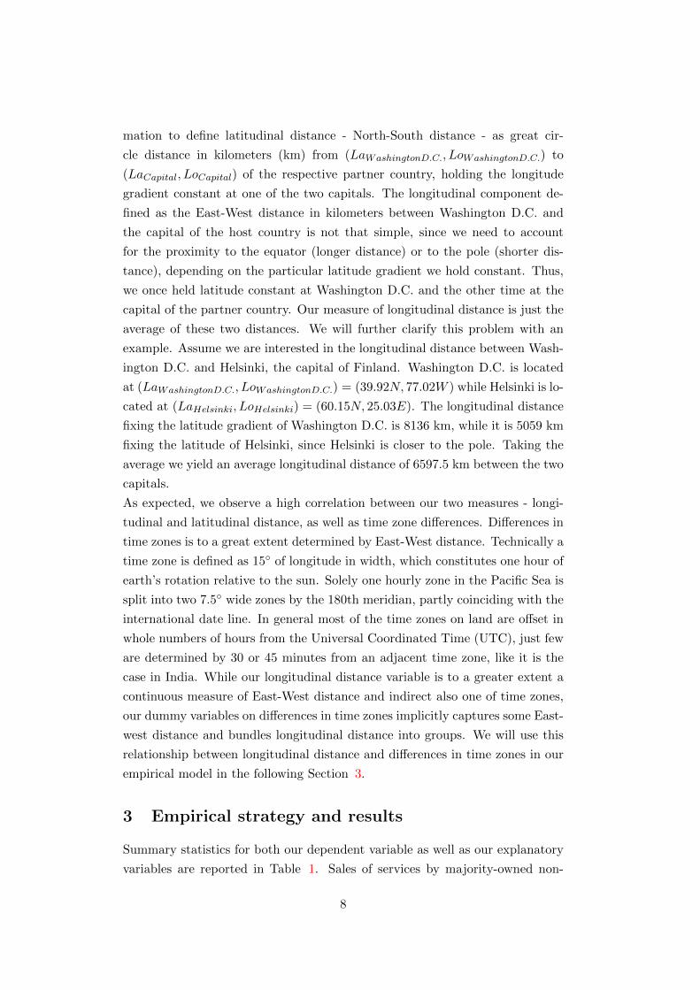
bounded between 2 to 15.428 and 38 to 9012 kilometers. Figure 1 shows the

development of affiliates sales over longitudinal distance.6 We can observe a

steadily increase of affiliate sales as we increase East-West distance, but the

increase is characterized by a stepwise function, indicating that specific values

of longitudinal distance have a greater impact on affiliate sales than others.

More interestingly, in a range of 5.000 to 6.000 kilometers we can observe 20%

to 60% of all affiliate sales, and about 80% of U.S. outward affiliate sales are

in a range of 10.000 kilometers. Regarding the variable measuring time zone

differences we see that the average partner country is located between five and

six time zones away from the east coast of the United States. Moreover only

few countries in our sample are landlocked and not surprisingly not adjacent

to the United States. However, more than a quarter of our partner countries

share the same language, English, as official language.

Figure 1: The development of affiliate sales over longitudinal distance

6We aggregated affiliates sales over all dimensions, partner countries, years and sectors

9

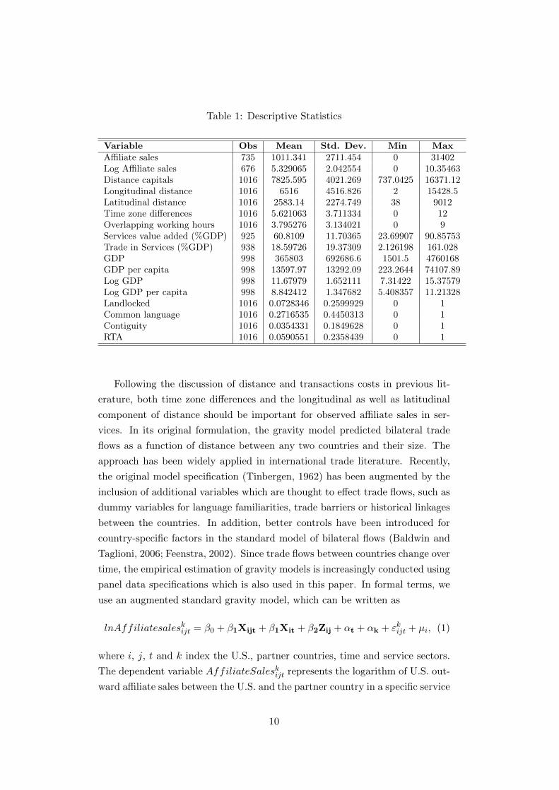
Table 1: Descriptive Statistics

Variable Obs Mean Std. Dev. Min MaxAffiliate sales 735 1011.341 2711.454 0 31402Log Affiliate sales 676 5.329065 2.042554 0 10.35463Distance capitals 1016 7825.595 4021.269 737.0425 16371.12Longitudinal distance 1016 6516 4516.826 2 15428.5Latitudinal distance 1016 2583.14 2274.749 38 9012Time zone differences 1016 5.621063 3.711334 0 12Overlapping working hours 1016 3.795276 3.134021 0 9Services value added (%GDP) 925 60.8109 11.70365 23.69907 90.85753Trade in Services (%GDP) 938 18.59726 19.37309 2.126198 161.028GDP 998 365803 692686.6 1501.5 4760168GDP per capita 998 13597.97 13292.09 223.2644 74107.89Log GDP 998 11.67979 1.652111 7.31422 15.37579Log GDP per capita 998 8.842412 1.347682 5.408357 11.21328Landlocked 1016 0.0728346 0.2599929 0 1Common language 1016 0.2716535 0.4450313 0 1Contiguity 1016 0.0354331 0.1849628 0 1RTA 1016 0.0590551 0.2358439 0 1

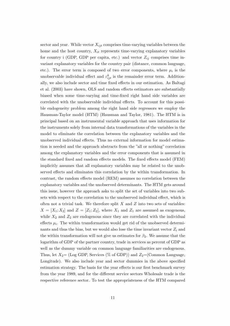
Following the discussion of distance and transactions costs in previous lit-

erature, both time zone differences and the longitudinal as well as latitudinal

component of distance should be important for observed affiliate sales in ser-

vices. In its original formulation, the gravity model predicted bilateral trade

flows as a function of distance between any two countries and their size. The

approach has been widely applied in international trade literature. Recently,

the original model specification (Tinbergen, 1962) has been augmented by the

inclusion of additional variables which are thought to effect trade flows, such as

dummy variables for language familiarities, trade barriers or historical linkages

between the countries. In addition, better controls have been introduced for

country-specific factors in the standard model of bilateral flows (Baldwin and

Taglioni, 2006; Feenstra, 2002). Since trade flows between countries change over

time, the empirical estimation of gravity models is increasingly conducted using

panel data specifications which is also used in this paper. In formal terms, we

use an augmented standard gravity model, which can be written as

lnAffiliatesaleskijt = β0 + β1Xijt + β1Xit + β2Zij + αt + αk + εkijt + µi, (1)

where i, j, t and k index the U.S., partner countries, time and service sectors.

The dependent variable AffiliateSaleskijt represents the logarithm of U.S. out-

ward affiliate sales between the U.S. and the partner country in a specific service

10

sector and year. While vector Xijt comprises time-varying variables between the

home and the host country, Xit represents time-varying explanatory variables

for country i (GDP, GDP per capita, etc.) and vector Zij comprises time in-

variant explanatory variables for the country pair (distance, common language,

etc.). The error term is composed of two error components, where µi is the

unobservable individual effect and εkijt is the remainder error term. Addition-

ally, we also include sector and time fixed effects in our estimation. As Baltagi

et al. (2003) have shown, OLS and random effects estimators are substantially

biased when some time-varying and time-fixed right hand side variables are

correlated with the unobservable individual effects. To account for this possi-

ble endogeneity problem among the right hand side regressors we employ the

Hausman-Taylor model (HTM) (Hausman and Taylor, 1981). The HTM is in

principal based on an instrumental variable approach that uses information for

the instruments solely from internal data transformations of the variables in the

model to eliminate the correlation between the explanatory variables and the

unobserved individual effects. Thus no external information for model estima-

tion is needed and the approach abstracts from the ”all or nothing” correlation

among the explanatory variables and the error components that is assumed in

the standard fixed and random effects models. The fixed effects model (FEM)

implicitly assumes that all explanatory variables may be related to the unob-

served effects and eliminates this correlation by the within transformation. In

contrast, the random effects model (REM) assumes no correlation between the

explanatory variables and the unobserved determinants. The HTM gets around

this issue, however the approach asks to split the set of variables into two sub-

sets with respect to the correlation to the unobserved individual effect, which is

often not a trivial task. We therefore split X and Z into two sets of variables:

X = [X1;X2] and Z = [Z1;Z2], where X1 and Z1 are assumed as exogenous,

while X2 and Z2 are endogenous since they are correlated with the individual

effects µi. The within transformation would get rid of the unobserved determi-

nants and thus the bias, but we would also lose the time invariant vector Zi and

the within transformation will not give us estimates for β2. We assume that the

logarithm of GDP of the partner country, trade in services as percent of GDP as

well as the dummy variable on common language familiarities are endogenous.

Thus, let X2= (Log GDP, Services (% of GDP)) and Z2=(Common Language,

Longitude). We also include year and sector dummies in the above specified

estimation strategy. The basis for the year effects is our first benchmark survey

from the year 1989, and for the different service sectors Wholesale trade is the

respective reference sector. To test the appropriateness of the HTM compared

11

to FEM, we apply a Hausman specification test. The test statistic of 6.36 is

less than the critical chi-squared value with five degrees of freedom at the 5%

significance level, so the null hypothesis is not rejected and the HTM is more

efficient. Testing of different specifications in previous literature, such as Egger

(2005), confirm our findings that the Hausman-Taylor approach seems to be the

most appropriate estimator for gravity models irrespective if we look on trade

in goods or services.

In our empirical approach we make use of both our measures for distance

- time zone differences as well as the latitudinal and longitudinal components

of distance. To capture the different impact of each variable, we employ three

different specifications that account for direct and indirect effects, as well as

non-linearities of our decomposed distance measures. In our first specification

we disentangle distance into a longitudinal and latitudinal component and look

at the direct impact of both of these distance measures on outward affiliate sales.

The results from our first specification following equation 1 using a Hausman-

Taylor approach are presented in column 1 of Table 2. We find a very consistent

positive impact of longitudinal and latitudinal distance on multinational activ-

ity. Our results suggest that both distance components are equally important

for affiliate sales and an increase in one of the two distance measures by 100

kilometers increases affiliates sales by 2%. In addition, our findings support

the importance of service transactions in terms of the value added content of

trade as previous papers have highlighted. Our dummy variables capturing the

geographical characteristics, like our contiguity and landlocked measures, have

both the expected sign. While being adjacent to the U.S. fosters affiliates sales,

being landlocked has a significant negative impact on the location of affiliates.

In contrast to previous findings, our measure for cultural ties, whether to coun-

tries share the same language, seems to have a negative effect on affiliate sales.

Surprisingly, our proxy for market size, GPD, is not significant at all. Our

control for the economic development has a positive impact on affiliates sales

and is significant at the 10% significance level. Our findings support our idea

that controlling for different service sectors is a necessary task. As our results

show, especially professional, scientific and technical services, as well as infor-

mation services rely heavily on interaction between provider and consumer and

on a local establishment. In finance and insurance services, where most of the

information exchange can be handled via online services, affiliates seem to be

of minor importance.

12

To account for differences in time zones as an alternative way to measure

East-West distance we pool hourly difference in time zones into specific groups

considering continents and geographical borders. In our baseline specification

we comprise the hourly time zone differences into five groups, whereby the ref-

erence group are all countries with zero time zone difference to Washington

D.C.. The first group summarizes all countries that are one to two time zones

away from the eats coast of the U.S.. The second group comprises all countries

with five to seven time zone differences, while the third group is determined by

eight and nine hours differences. The last group includes all countries with a

time zone difference of ten hours or more. The results from our baseline second

specification using the five groups of pooled time zone difference variables are

reported in column 1 of Table 3. In addition to these five groups of pooled

time zone differences we use alternative thresholds to group the countries with

respect to their time zone. These results are presented in in column 2 to 4 of

Table 3. As we can see from our baseline model in column 1 being further away

in terms of time zones raises affiliate sales compared to our reference group with

no time zone difference. Across all approaches a time zone difference of 1 or

2 hours has no significant impact on affiliate sales compared to the baseline.

However, crossing the Atlantic Sea and bearing a time zone difference or more

than 5 hours significantly raises the need for an affiliate, although our find-

ings suggest that there is no impact in the time zone group of 8 to 9 hours in

compared to our reference group. If we consider different specification of the

pooled time zones our results remain robust across the various specifications.

In the most detailed analysis in column 3 of Table 3 our findings suggest that

there exist special ranges in which time zone differences are more important.

It seems that that we can observe three natural thresholds, 5 to 6 hours, 9 to

10.5 hours and 11 to 12 hours, which raise the cost of doing business abroad.

The first group to a great extent summarizes all Western and Central European

countries that are across the Atlantic sea, where interaction between providers

and consumers is hampered by time zone differences and travel involves a long-

distance flight. Our second group is bearing a hourly time zone difference of 9

to 10.5 hours, which means almost no overlap in business working hours and

severe problems for real time communication. The last group with more than

11 hours constitutes the group with the highest distance to the United States

and thus higher transaction costs enhance the level of affiliate activity in this

areas. Regarding our North-South distance component the impact of latitudinal

distance remains robust compared to our first specification. An increase of 100

kilometers in North-South distance raises affiliate sales by 3%. The logarithm

13

of GDP per capita, our control for the economic development of a country, has

a significantly positive effect on affiliate sales in all estimations. Additionally,

affiliate sales are driven by a higher extent of value added content of trade. Our

variables controlling for other determinants that influence transactions costs

again remain robust to our first specification and have the expected sign, ex-

cept for the dummy on language familiarities. Our findings in Table 3 again

confirm our proposition that we need to control for the nature of services, by

using sector specific dummy variables. We find a significantly positive impact

of the different service sectors compared to our baseline and the impact across

service sectors is varying. Again the strongest impact can be found for profes-

sional, scientific an technical services.

Our second specification is in addition extended to take in account the pos-

sibility of non-linear effects of time zones by using dummy variables for every

time zone difference in our data set. Using groups of time zone differences we

implicitly assume that the impact of time zone differences varies across differ-

ent groups of hourly differences, but is the same within the specified group. In

practise this specifications assumes that for instance the impact in time zone

differences across Europe is the same, independently if we operate an affiliate

in Great Britain that is five hours away from the east coast of the U.S. or in

Poland that involves a time zone difference of six hours. Moreover, also when

we introduce dummy variables for each time zone difference we implicitly do not

take into account the possible longitudinal distance between partner countries

in the same time zone, like it is the case for Finland and South Africa. We

address this issue in two ways. First, we include both measures longitudinal

and latitudinal distance component as well as groups of time zone differences

as we have done in our second specification and account for an impact of longi-

tudinal distance within a time zone more precisely in a spline regression model

that we employ in our third specification. Based on the groups of differences in

time zones we specify threshold values, so-called knots, in terms of longitudinal

distance. As in specification two we comprise the hourly time zone differences

into five groups and define the knots as the minimal longitudinal distance in

each group.

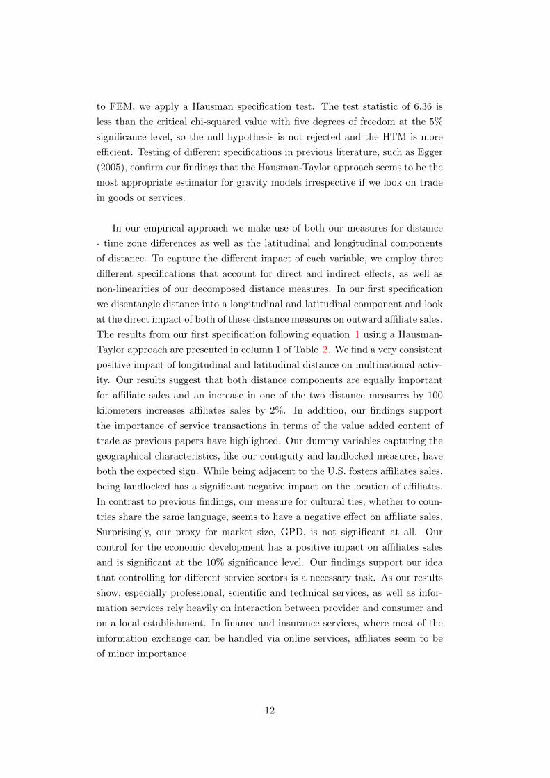
Controlling for non-linear effects of time zones by using dummy variables

for every time zone difference our results support the idea that some time zones

are more important compared to others. As column 2 of Table 2 shows being

away one hour or two in terms of time zones does not have a significant impact

14

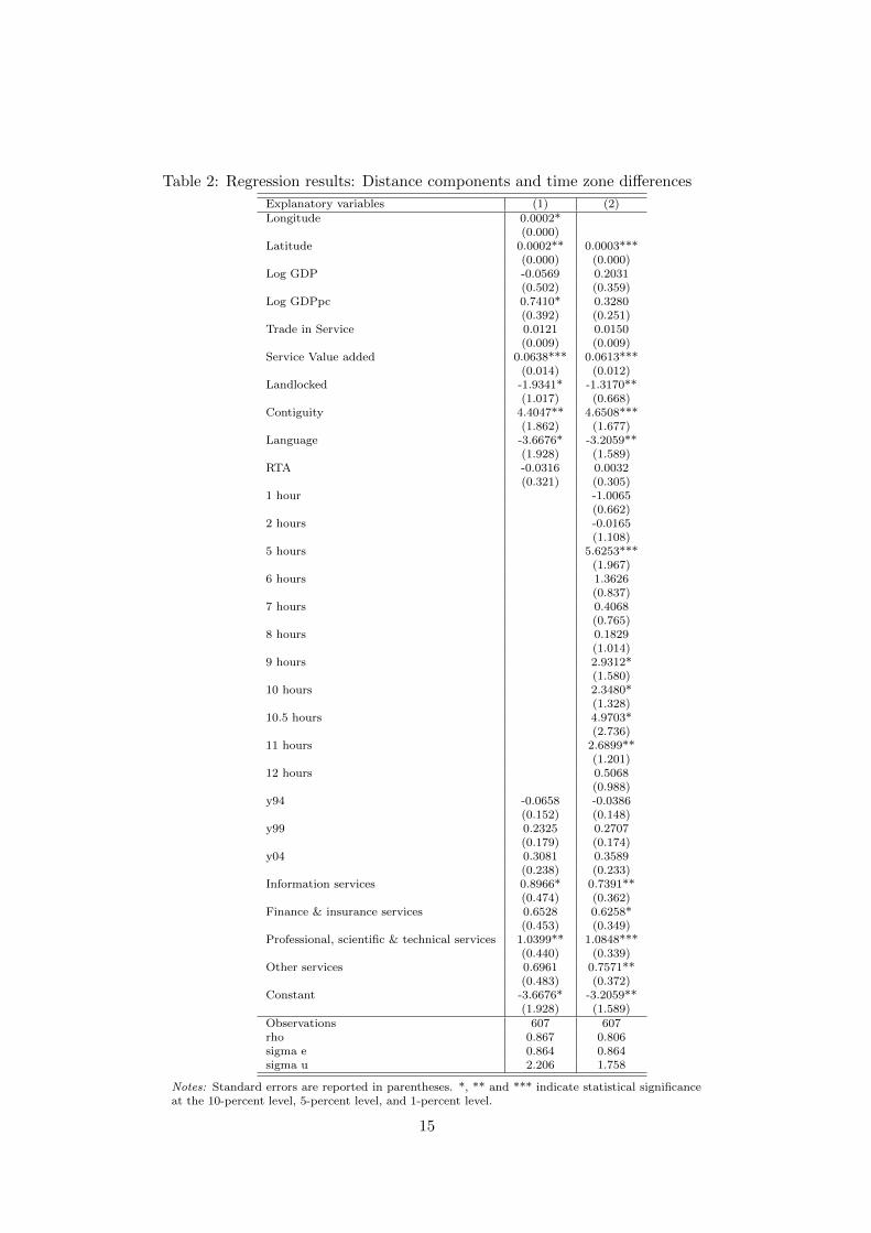
Table 2: Regression results: Distance components and time zone differences

Explanatory variables (1) (2)Longitude 0.0002*

(0.000)Latitude 0.0002** 0.0003***

(0.000) (0.000)Log GDP -0.0569 0.2031

(0.502) (0.359)Log GDPpc 0.7410* 0.3280

(0.392) (0.251)Trade in Service 0.0121 0.0150

(0.009) (0.009)Service Value added 0.0638*** 0.0613***

(0.014) (0.012)Landlocked -1.9341* -1.3170**

(1.017) (0.668)Contiguity 4.4047** 4.6508***

(1.862) (1.677)Language -3.6676* -3.2059**

(1.928) (1.589)RTA -0.0316 0.0032

(0.321) (0.305)1 hour -1.0065

(0.662)2 hours -0.0165

(1.108)5 hours 5.6253***

(1.967)6 hours 1.3626

(0.837)7 hours 0.4068

(0.765)8 hours 0.1829

(1.014)9 hours 2.9312*

(1.580)10 hours 2.3480*

(1.328)10.5 hours 4.9703*

(2.736)11 hours 2.6899**

(1.201)12 hours 0.5068

(0.988)y94 -0.0658 -0.0386

(0.152) (0.148)y99 0.2325 0.2707

(0.179) (0.174)y04 0.3081 0.3589

(0.238) (0.233)Information services 0.8966* 0.7391**

(0.474) (0.362)Finance & insurance services 0.6528 0.6258*

(0.453) (0.349)Professional, scientific & technical services 1.0399** 1.0848***

(0.440) (0.339)Other services 0.6961 0.7571**

(0.483) (0.372)Constant -3.6676* -3.2059**

(1.928) (1.589)Observations 607 607rho 0.867 0.806sigma e 0.864 0.864sigma u 2.206 1.758

Notes: Standard errors are reported in parentheses. *, ** and *** indicate statistical significanceat the 10-percent level, 5-percent level, and 1-percent level.

15

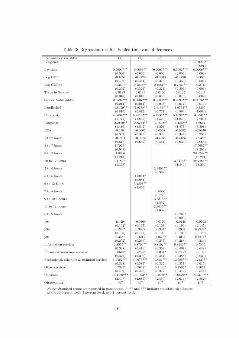
Table 3: Regression results: Pooled time zone differences

Explanatory variables (1) (2) (3) (4) (5)Longitude -0.0021*

(0.001)Latitude 0.0003*** 0.0003** 0.0003*** 0.0003*** 0.0006***

(0.000) (0.000) (0.000) (0.000) (0.000)Log GDP -0.1054 -0.2128 -0.0008 -0.1790 0.6073

(0.432) (0.461) (0.373) (0.455) (0.609)Log GDPpc 0.7360** 0.7836** 0.4661** 0.7753** -0.2911

(0.292) (0.304) (0.221) (0.303) (0.606)Trade in Service 0.0123 0.0131 0.0140 0.0125 0.0144

(0.010) (0.010) (0.010) (0.010) (0.009)Service Value added 0.0597*** 0.0607*** 0.0580*** 0.0597*** 0.0676***

(0.014) (0.014) (0.013) (0.014) (0.013)Landlocked -1.8459** -2.0278** -2.1155*** -1.9763** 0.3390

(0.816) (0.875) (0.771) (0.864) (1.604)Contiguity 4.8687*** 5.2516*** 4.7931*** 5.1697*** 4.3341**

(1.741) (1.855) (1.579) (1.843) (2.200)Language -3.2129** -3.6774** -2.7602** -3.4248** 1.6614

(1.416) (1.542) (1.224) (1.477) (3.291)RTA -0.0104 -0.0002 0.0308 -0.0092 -0.0940

(0.339) (0.346) (0.328) (0.344) (0.296)1 to 2 hours -0.3911 -0.3972 -0.4061 -0.4185 2.9495

(0.617) (0.642) (0.561) (0.633) (2.083)5 to 7 hours 1.7027* 17.0652**

(0.931) (8.203)8 to 9 hours 1.8696 20.8242**

(1.213) (10.201)10 to 12 hours 3.1180** 3.3476** 29.7285**

(1.368) (1.440) (14.290)5 to 6 hours 2.4493**

(0.992)5 to 8 hours 1.8001*

(0.981)9 to 12 hours 3.4803**

(1.460)7 to 8 hours 0.6960

(0.785)9 to 10.5 hours 3.6313**

(1.552)11 to 12 hours 2.3616**

(1.008)5 to 9 hours 1.8765*

(0.999)y94 -0.0294 -0.0100 0.0170 -0.0148 -0.0192

(0.162) (0.167) (0.161) (0.166) (0.145)y99 0.2707 0.3035 0.3387* 0.2932 0.2944*

(0.188) (0.197) (0.190) (0.195) (0.175)y04 0.3687 0.4211 0.4675* 0.4035 0.4274*

(0.252) (0.266) (0.257) (0.263) (0.234)Information services 0.8555** 0.8799** 0.8102** 0.8643** 0.7535

(0.398) (0.416) (0.362) (0.407) (0.649)Finance & insurance services 0.6640* 0.6726* 0.6031* 0.6712* 0.5195

(0.379) (0.396) (0.344) (0.388) (0.630)Professional, scientific & technical services 1.0562*** 1.0673*** 1.0681*** 1.0585*** 1.2133**

(0.368) (0.385) (0.335) (0.377) (0.615)Other services 0.7387* 0.7649* 0.7146* 0.7504* 0.9074

(0.409) (0.428) (0.372) (0.419) (0.674)Constant -6.4380*** -5.7023** -5.4638** -6.0629** -8.5376***

(2.497) (2.685) (2.550) (2.614) (2.887)Observations 607 607 607 607 607

Notes: Standard errors are reported in parentheses. *, ** and *** indicate statistical significanceat the 10-percent level, 5-percent level, and 1-percent level.

16

on affiliates sales compared to our base group with zero hourly difference. But

we find a strong positive impact of being away five hours in terms of time zones.

This means that as soon as distance or the difference in time zones increases

significantly, the cost burden of trade in services in terms of higher transaction

costs seems to foster affiliate sales. Further, our findings show that time zone

differences of nine to eleven hours significantly raise affiliate sales again com-

pared to our reference group. Especially countries in these areas suffer from

high transaction cost due to a few or no overlapping in working hours and high

distances to the United States. Our maximum time zone difference of 12 hours,

where we can observe only few countries in our sample, has no significant im-

pact. Our coefficients for the other variables remain robust compared to our

first specification. In addition to our first model, all service sector dummies

suggest a significantly positive impact on affiliate sales in comparison to our

baseline group.

To account for the varying longitudinal distance within one group of pooled

time zone differences we extend our second specification by including longitudi-

nal as well as latitudinal distance in addition to the groups of time zones from

our basic specification (see column 1 of Table 3). The results are presented in

column 5 of Table 3. By including latitudinal distance in addition to the pooled

time zone difference the coefficient of longitudinal distance turns negative and

is significantly different from zero at the 10% significance level. Increasing lon-

gitudinal distance by 100 kilometers reduces affiliate sales by 20%. However,

this negative impact of East-West distance is offset by the significantly positive

effect of the pooled time zones. Being away more than five hours in terms of

time zone differences to the U.S. increases affiliates sales significantly compared

to our reference group. Interestingly, the impact within a time zone increases

steadily the more time zones we have to take into account. Reversing the in-

terpretation of these two measures we can say that being further away in time

zones significantly raises affiliate sales, although accounting for the actual East-

West distance our findings suggest that adding one kilometer to the East-West

distance harms affiliate sales by 0.2%. Our measure for North-South distance

remains robust, although the impact of latitudinal distance increased compared

to our first specification to 6% for an additional distance of 100 kilometers.

With respect to our other explanatory variables the results are robust across

the various specifications.

To account for an impact of longitudinal distance within a time zone more

precisely we employ a spline regression model as our third specification. Based

17

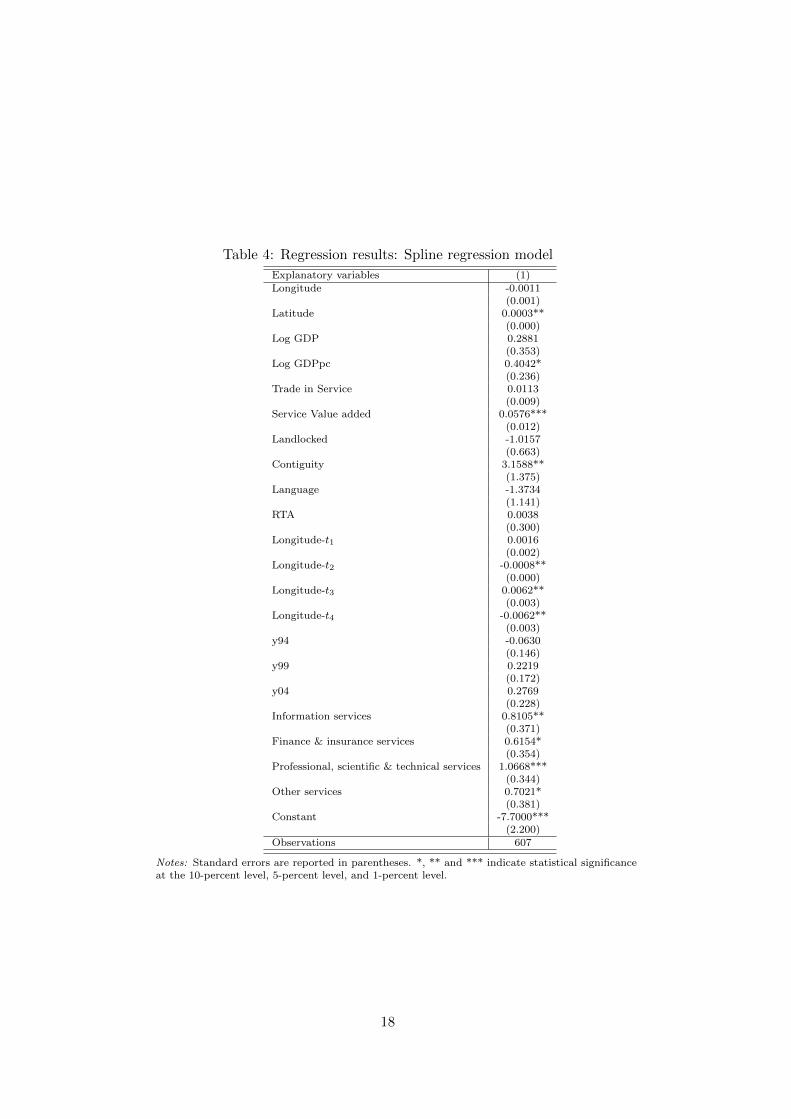
Table 4: Regression results: Spline regression model

Explanatory variables (1)Longitude -0.0011

(0.001)Latitude 0.0003**

(0.000)Log GDP 0.2881

(0.353)Log GDPpc 0.4042*

(0.236)Trade in Service 0.0113

(0.009)Service Value added 0.0576***

(0.012)Landlocked -1.0157

(0.663)Contiguity 3.1588**

(1.375)Language -1.3734

(1.141)RTA 0.0038

(0.300)Longitude-t1 0.0016

(0.002)Longitude-t2 -0.0008**

(0.000)Longitude-t3 0.0062**

(0.003)Longitude-t4 -0.0062**

(0.003)y94 -0.0630

(0.146)y99 0.2219

(0.172)y04 0.2769

(0.228)Information services 0.8105**

(0.371)Finance & insurance services 0.6154*

(0.354)Professional, scientific & technical services 1.0668***

(0.344)Other services 0.7021*

(0.381)Constant -7.7000***

(2.200)Observations 607

Notes: Standard errors are reported in parentheses. *, ** and *** indicate statistical significanceat the 10-percent level, 5-percent level, and 1-percent level.

18

on the longitudinal distance determining the groups of time zone differences (as

we have specified them in our second specification) - 1to 2 hours, 5 to 7 hours,

8 to 9 hours and 10 to 12 hours - we define threshold values. To make the

function piecewise continuous we require that the segments join at the knots.

Table 4 reports our results from the spline regression model where we can show

that the impact of longitudinal distance within a time zone is varying. Our

results suggest that our measure for longitude distance in the base scenario

with zero hourly differences in time zones is negative, however not significant.

Increasing longitudinal distance and moving to the group of countries with 1

or 2 hours of time zone difference the impact on affiliates sales is positive, but

again insignificant. Interestingly, if we move further to our group with 5 to

7 hours of time zone differences our findings show a significant negative effect.

The effect is positive and significant if we increase longitudinal distance and the

number of time zone differences to 8 and 9 hours and turns negative again if we

exceed a time zone difference of 10 hours. Our results suggest that the impact

is quite ambiguous within a group of time zones. While increasing longitudinal

distance once we passed the 5 hours threshold has negative effects, the impact

of increasing distance is positive for the group with an hourly difference of 8

and 9 hours. The reason for this may build upon our argument that particu-

lar distances and time zones are disadvantageous with respect to traveling and

real time communication and therefore require a heavier dose of multinational

activity. Regarding the results on the other explanatory variables our findings

to do not change much with respect to our first specification.

Overall, our specifications allow the conclusion that the results are quite

robust and the methodology used is appropriate for our research question. This

leads to a discussion of possible limitations of our study. Due to data limita-

tions for affiliate sales statistics our study is based on U.S. outward affiliate

sales, where the U.S. represents the only source country. Clearly, our research

design would be enriched if we could build upon bilateral foreign affiliate sales

data. Nevertheless, our empirical approach tries to overcome these caveats and

to incorporate a model that does account for our data issues. Future research

questions in this kind of area could include the impact of distance components

and time zone differences in goods trade in comparison to trade in services. Ad-

ditionally, one could raise the question of how services off-shoring is determined

by time zones and to what extent the advantages of time zone differences that

allows for working around the clock are implemented.7

7See Kikuchi and Marjit (2010) for a theoretical discussion of this question.

19

4 Conclusions

In this paper we focus on the impact of distance and time zone differences on

trade in services through foreign affiliates. We offer a alternative way to mea-

sure distance in terms of transactions cost. Hence, we decompose distance into a

longitudinal and latitudinal component to capture East-West and North-South

distance separately. Additionally, as an alternative measure we use differences

in time zones to account for difficulties in real time interaction necessary for the

provision of certain services. Due to the need for proximity factors like distance

place an additional cost burden on some forms of service delivery. Additionally,

time zone differences add significantly to the cost of doing business abroad.

Both measures of transaction costs appear empirically robust in explaining in-

creased affiliate sales. By increasing longitudinal or latitudinal distance by 100

kilometers affiliate sales increase by 2%. Our findings on increased time zone

differences confirm this proximity burden. By moving further away from the

Unites States in terms of time zones we find a significantly positive impact

on affiliate sales for time zone differences of 5 hours and 9 or more hours. The

value added content of services trade as well as the economic development of the

partner countries enhance affiliates sales additionally. Due to the heterogenous

nature of services our results support our proposition that we have to account

for various service sectors. We find that foreign affiliates especially play a im-

portant role for information intensive services, such as professional, scientific

and technical as well as information services.

20

References

Baldwin, R. E., Taglioni, D., 2006. Gravity for dummies and dummies for grav-ity equations. CEPR Discussion Paper No. 5850.

Baltagi, B., Bresson, G., Pirotte, A., 2003. Fixed effects, random effects orhausman taylor?: A pretest estimator. Economic Letters 79, 361–369.

Christen, E., Francois, J., 2010. Modes of delivery in services. CEPR DiscussionPaper No. 7912.

Egger, P., 2005. Alternative techniques for estimation of cross-section gravitymodels. Review of International Economics 13 (5), 881–891.

Feenstra, R., 2002. Border effects and the gravity equation: Consistent methodsfor estimation. Scottish Journal of Political Economy 49(5), 491 – 506.

Francois, J., Manchin, M., 2011. Services linkages and the value added contentof trade. Washington DC: World Bank working paper.

Francois, J. F., Hoekman, B., 2010. Services trade and policy. Journal of Eco-nomic Literature forthcoming.

Grunfeld, L. A., Moxnes, A., 2003. The intangible globalization: Explaining thepatterns of international trade in services. Norwegian Institute for Interna-tional Affairs. Working Paper No. 657 - 2003.

Hattari, R., Rajan, R., 2008. Sources of fdi flows to developing asia: The rolesof distance and time zones. ADB Institute Working Paper No. 117.

Hausman, J., Taylor, W., 1981. Panel data and unobservable individual effects.Econometrica 49, 1377–1398.

Kamstra, M., Kramer, l., Levi, M., 2000. Losing sleep at the marklet: Thedaylight-savings anomaly. American Economic Review 90 (4), 1005–1011.

Kikuchi, T., Marjit, S., 2010. Time zones and periodic intra-industry trade.EERI Research Paper Series No. 08/2010.

Kolstad, I., Villanger, E., 2008. Determinats of foreign direct investment inservices. European Journal of Political Economy 24, 518 – 533.

Loungani, P., Mody, A., Razin, A., 2002. The global disconnect: the role oftransactional distance and scale economies in gravity equations. ScottishJournal of Political Economy 49(5), 526–543.

Mayer, T., Zignago, S., 2006. Notes on cepii’s distances measures. CEPII, Paris.

Portes, R., Rey, H., 2005. The determinats of cross-border equity flows. Journalof International Economics 65, 269–296.

Stein, E., Daude, C., 2007. Longitude matters: Time zones and the location offoreign direct investment. Journal of International Economics 71, 96–112.

21

Tinbergen, J., 1962. Shaping the World Economy: Suggestions for an Interna-tional Economic Policy. New York: Twentieth Century Fund.

U.S. Bureau of Economic Analysis, 2008. U.S. Direct Investment Abroad: 2004Final Benchmark Data. Washington, DC: U.S. Government Printing Office,November 2008.

22