Embed Size (px)
Citation preview

Time Variation of the Equity Term Structure
Niels Joachim Gormsen⇤
First draft September 2016. This version December 2017
Please Click Here for Latest Version
Abstract
I document that the term structure of holding-period equity returns is counter-
cyclical: it is downward sloping in good times, but upward sloping in bad times.
This new stylized fact implies that long-maturity risk plays a central role in asset
price fluctuations, consistent with theories of long-run risk and habit, but these
theories cannot explain the average downward slope. At the same time, the cycli-
cal variation is inconsistent with recent models constructed to match the average
downward slope. I present the theoretical source of the puzzle and suggest a new
model as a resolution. My model also shows that the counter-cyclical term struc-
ture has implications for real activity, which I verify empirically: in bad times,
long-duration firms decrease their investment and capital-to-labor ratio relative to
short-duration firms.
Keywords: asset pricing, equity term structure, time-varying discount rates.
JEL classification: G10, G12.
⇤I am grateful for helpful comments from John Y. Campbell, Robin Greenwood, Sam Hanson, RalphKoijen (discussant), Eben Lazerus, Matteo Maggiori, Lasse Heje Pedersen, Andrei Shleifer, JeremyStein, Adi Sunderam, and Paul Whelan, as well as participants at the NFN conference. I gratefullyacknowledge support from the European Research Council (ERC grant no. 312417) and the FRICCenter for Financial Frictions (grant no. DNRF102). I am a PhD Student at Copenhagen BusinessSchool, Department of Finance. Email: [email protected].

I study the term structure of equity returns and document a large cyclical variation.
This cyclical variation is important for understanding which risks drive fluctuations
in asset prices. Indeed, the cyclical variation documented in this paper suggests that
price fluctuations are driven mainly by long-maturity risks such as persistent changes in
dividend growth, and only less by short-maturity risks such as disaster risks. As such, the
results are consistent with classical asset pricing models such as Campbell and Cochrane
(1999) or Bansal and Yaron (2004), but they are inconsistent with the newer models
that are designed to have downward sloping equity term structures. In addition, the
cyclical variation of the equity term structure has important real consequences because
it directly influences when capital flows to long-maturity firms such as biotech firms or
short-maturity firms such as automobile firms and the extent to which these firms invest
in production plants, R&D, or labor.
By way of background, the previous research on the equity term structure has focused
on its average slope, finding that it is downward sloping on average (Binsbergen, Brandt,
and Koijen, 2012), as indicated by the solid line in my Figure 1. This result is inconsistent
with traditional models of long-run risk and habit which have upward sloping term
structures. Addressing this challenge to traditional asset pricing models has become
one of the most active areas in macro-finance (Cochrane, 2017) and has led to the
development of new models with average downward sloping term structures.1
I contribute to the literature on the equity term structure by studying its time
variation. My main result is that the equity term structure of holding-period returns
is counter-cyclical: it is downward sloping in good times but upward sloping in bad
times. As shown in Figure 1, this counter-cyclical variation is economically large. In
good times, long-maturity equity has 4 percent lower expected annual return than short-
maturity equity, but in bad times it has 5 percent higher expected return, meaning that
1The reference model for a downward sloping term structure is Lettau and Wachter (2007), whichprecedes the empirical literature on the downward sloping equity term structure. More recent modelsinclude Eisenbach and Schmalz (2013); Andries, Eisenbach, and Schmalz (2015); Nakamura, Steinsson,Barro, and Ursua (2013); Belo, Collin-Dufresne, and Goldstein (2015); Croce, Lettau, and Ludvigson(2014); Hasler and Marfe (2016). Binsbergen and Koijen (2017) review the new theoretical models thathave been motivated by the downward sloping terms structure.
1

Figure 1: The Term Structure of One-Year Equity Returns
This figure shows the term structure of holding-period equity returns for the S&P 500. The figureshows the unconditional average return (solid line), the average return in bad times (dashed line), andthe average return in good times (dash-dotted line). Good and bad times are defined by the ex antedividend-price ratio. Short-maturity equity claims is the average return to dividend futures of 1 to 7years maturity. The long-maturity claim is the average return to the market portfolio. Returns areannual spot returns, 2005 – 2016.
the equity term premium varies by 9 percentage points between good and bad times.
As shown in Figure 2, I document this new stylized fact using several di↵erent mea-
sures of term premia, sample periods, data sources, and by also using futures returns
as opposed to spot returns. Using dividend futures with maturities up to seven years,
I find a positive relation between the ex ante dividend price ratio and the ex post one-
year return di↵erence between long- and short-maturity dividend futures (Panel A). The
result also holds when using the market portfolio as the long-maturity claim, when con-
sidering Sharpe ratios instead of returns, when excluding the financial crisis, and when
using other measures of bad times such as the CAPE ratio and the cay variable. The
result holds in the U.S. for the S&P 500 and it holds internationally for Nikkei 225, Euro
Stoxx 50, and the FTSE 100. Going beyond dividend futures, the result also holds when
2

measuring the equity term structure using option implied dividend prices (Panel B) or
the cross-section of stocks (Panel C).2
As shown in the first two columns of Table 1, the counter-cyclical equity term pre-
mia represent a puzzle for asset pricing theory: none of our canonical asset pricing
models are able to produce both the counter-cyclical variation documented in this pa-
per and the negative slope documented by Binsbergen, Brandt, and Koijen (2012). The
counter-cyclical variation is consistent with the traditional macro-finance models such as
Campbell and Cochrane (1999) and Bansal and Yaron (2004), but inconsistent with the
new models with average downward sloping term structures. Hence, traditional models
explain the time-variation in the term premium, but not its average value, and vice versa
for the newer models.
The puzzle applies more generally than just the models in Table 1. To underline
the generality of the puzzle and to identify its source, I study the cyclicality of term
premia through a simple, essentially a�ne model that is su�ciently general to capture
most of the dynamics of log-normal models. In the model, the term structure of returns
may be either upward or downward sloping; but I show that if it is upward sloping it
is counter-cyclical and if it is downward sloping it is pro-cyclical. To see the intuition
behind this result, consider for instance a downward sloping model. The downwards
sloping term structure suggests that short-maturity equity is riskier than long-maturity
equity and commands a premium, meaning that the equity term premium is negative.
In bad times, this premium on short-maturity equity increases because the price of risk
increases and the term premium thus becomes even more negative, not positive as is
observed empirically.
To understand what is needed to resolve the puzzle and explain the stylized facts, I
introduce a new model with a term premium that is both counter-cyclical and negative
on average. In the model, investors trade o↵ a demand for hedging investment oppor-
tunities with an aversion towards long-run risk: the required return on long-maturity
2I estimate a term-premium mimicking portfolio in the cross-section of stocks by projecting theexcess returns of characteristics-sorted portfolios onto the realized return di↵erence between long- andshort-maturity claims.
3

equity is pushed down by investors’ demand for hedging investment opportunities, but it
is pushed up by their aversion for long-run risk. The relative strength of the two e↵ects
varies over time, and the model is specified such that demand for hedging dominates on
average, meaning that the equity term premium is negative on average; but in bad times
the aversion against long-run risk dominates so that the equity term premium becomes
positive. The model is thus able to capture the two stylized facts of the equity term
structure. The model is based on an exogenous stochastic discount factor and rooting
it in a micro-foundation remains an interesting topic for future research.
The counter-cyclical term premia documented in this paper may be surprising given
the pro-cyclical ”equity yield curve” documented by Binsbergen, Hueskes, Koijen, and
Vrugt (2013). An equity yield is the current dividends divided by the price of future
dividends of a given maturity, meaning that it is closely related to hold-to-maturity
returns.3 The authors document that the yield curve is steeply downward sloping in bad
times, which might lead one to believe that during bad times, long-maturity claims are
expected to have low returns relative to short maturity claims, i.e. that the one-period
equity term premium is lower than usually. However, I directly study the one-period
term premium and find that it is higher in bad times, even though the yield curve is
downward sloping.
To better understand this negative relation between equity term premia and the slope
of the yield curve, I test an expectations hypothesis. The hypothesis is that equity term
premia are constant, meaning that the expected development in yields can be inferred
from the yield curve. I find that equity yields move in the direction suggested by the
yield curve, but they move by more than suggested by the expectations hypothesis. I
show that this excess movement in yields implies that the slope of the equity yield curve
must be negatively correlated with equity term premia, thus reconciling my results with
Binsbergen, Hueskes, Koijen, and Vrugt (2013). The result that yields move too much
in the direction of what the yield curve suggests is surprising because it contrasts the
results from the bond literature: for bonds, the expectations hypothesis is rejected
3Equity yields are equivalent to hold-to-maturity returns minus the hold-to-maturity growth rates.
4

because yields move in the opposite direction of what the yield curve suggests4.
In addition, the test of the expectations hypothesis represents another tension be-
tween theory and the data. As shown in the third column of Table 1, none of the asset
pricing models I consider are able to generate as strong a relation between the yield
spread and future changes in yields as that observed in the data. The models fail in
this regard because their term premium is pro-cyclical or because the models create too
little predictability in equity yields relative to term premia.
Finally, the counter-cyclical equity term structure is also important for understanding
the cost of capital and how real resources are allocated in the economy. To better
understand these real dynamics, I study firms‘ investment decisions in my model of the
equity term structure. In the model, some firms have long-maturity cash flows and some
have short-maturity. These firms are di↵erently a↵ected by the equity term structure:
in bad times, the counter-cyclical equity term structure incentivizes long-maturity firms
to invest less and to apply less capital relative to labor compared to short-maturity firms
because the long-maturity firms find capital relatively more expensive.
I verify the real implications of the model empirically, as summarized in Figure 3.
I find that, in bad times, the long-maturity firms invest less in capital equipment and
R&D than short-maturity firms do. On the other hand, they increase spending on wages
relative to short-maturity firms. Taken together, the long-maturity firms thus decrease
their capital to labor ratio relative to short-maturity firms. This pattern is consistent
with long-maturity firms finding capital relatively more expensive than short-maturity
firms do in bad times because the equity term structure is more upward sloping.
In conclusion, this paper documents a new stylized fact that gives new insight into
the drivers of the equity risk premium. The counter-cyclical term structure implies that
the variation in the equity risk premium mainly comes from variation in long-term risk.
Together with the observation that the equity term structure is downward sloping, the
counter-cyclical term structure represents a puzzle for existing macro-finance models.
I show theoretically that the canonical models are not able to reproduce both facts,
4See e.g. Shiller (1979); Shiller, Campbell, and Schoenholtz (1983) and Campbell and Shiller (1991).
5

and as a response I introduce a new model that can. Finally, I show empirically and
theoretically that the cyclicality of the equity term structure is linked to the cylicality
in real investments: in bad times where the equity term structure is upward sloping,
long-maturity firms invest less than short-maturity firms.
The paper proceeds as follows. Section I introduces a model of the equity term struc-
ture with implications for firm investment. Section II describes data sources. Section III
documents the counter-cyclical equity term structure. Section IV tests the expectation
hypothesis. Section V studies real consequences of the equity term structure. Section
VI studies calibrations of several canonical asset pricing models individually as well as
my model introduced in section II. Section VII concludes.
1 Motivating Theory
In this section, I introduce a simple extension of the model of the equity term structure
by Lettau and Wachter (2007). In the special case of the original Lettau and Wachter
model, I show that there is a link between the sign and cyclicality of the term premium
in the sense that term premia are either positive on average and counter-cyclical or
negative on average and pro-cyclical (Proposition 1.a). In the more general version of
the model, one can capture the empirical regularities that I uncover, that is, one can
have term premia that are negative on average and counter-cyclical (Proposition 1.b).
Finally, I study the link between the equity term structure and the investment decisions
of individual firms, finding that long-maturity firms use less capital to labor when the
equity term structure is more upward sloping (Proposition 2).
1.1 Model
The economy has an aggregate equity claim with dividends at time t denoted by Dt,
where dt = ln(Dt) evolves as
�dt+1 = µg + zt + �d✏d,t+1 (1)
6

Here µg 2 R is the unconditional mean dividend growth and zt drives the conditional
mean:
zt+1 = 'zzt + �z✏z,t+1 (2)
where 0 < 'z < 1. Further, ✏d,t+1 and ✏z,t+1 are normally distributed mean-zero shocks
with unit variance and �d, �z are their volatilities.
The risk-free rate rf is constant and the stochastic discount factor is given by
Mt+1 = exp
✓�rf � 1
2x2t � xt✏d,t+1 � a
✓1
2a+ xt⇢dx + ✏x,t+1
◆◆(3)
where a 2 R and the state variable xt drives the price of risk:
xt+1 = (1� 'x)x+ 'xxt + �x✏x,t+1 (4)
The parameter x 2 R+ is the long-run average, 0 < 'x < 1, and ✏x,t+1 is a normally
distributed mean-zero shock with unit variance and �x is the volatility. The three shocks
have correlations denoted ⇢dx, ⇢dz, and ⇢zx, where ⇢zx = 0, ⇢dx�x 'x, and ⇢dz�z <
�d(1 � 'z). The first assumption is also made by Lettau and Wachter (2007) and the
latter two hold in their empirical calibration.
To understand the intution behind the stochastic discount factor, consider first the
case where a = 0 as in Lettau and Wachter (2007). In this case, investors are averse
towards shocks to dividends, ✏d,t+1. A negative shock to dividends increases the marginal
utility and thus increases the value of the stochastic discount factor. The e↵ect of a given
shock on the stochastic discount factor depends on the price-of-risk variable xt, which
in this sense can be interpreted as a risk aversion variable. In addition, shocks to the
price of risk and the conditional growth rate zt are only priced to the extent that they
are correlated with the dividend shock, which is consistent with, for instance, the habit
model.
In the more general case where a 6= 0, the price-of-risk shock is priced even if it
7

is uncorrelated with the dividend shock. If, for instance, a < 0, investors are averse
towards increases in the price of risk. The intuition behind such a specification is that
an increase in the price of risk causes a capital loss today, which increases marginal
utility. The shock to the price of risk is scaled by a and not by the price of risk, meaning
that the aversion towards the price-of-risk shocks are constant over time.5
1.2 Equity Term Premia and Their Cyclicality
The analysis is centered around the prices and returns on n-maturity dividend claims.
The price of an n-maturity claim at time t is denoted P nt and the log-price is denoted
pnt = ln(P nt ). Since an n-maturity claim becomes and n� 1 maturity claim next period,
we have the following relation for prices:
P nt = Et
⇥Mt+1P
n�1t+1
⇤(5)
with boundary condition P 0t = Dt because the dividend is paid out at maturity. To
solve the model, I conjecture and verify that the price dividend ratio is log-linear in the
state variables zt and xt:
P nt
Dt= exp (An +Bn
z zt +Bnxxt) (6)
The price dividend ratio can then be written as
P nt
Dt= Et
Mt+1
Dt+1
Dt
P n�1t+1
Dt+1
�= Et
Mt+1
Dt+1
Dtexp
�An�1 +Bn�1
z zt+1 +Bn�1x xt+1
��(7)
5These dynamics are reminiscent of the long-run risk model. In the long-run risk model, the coun-terpart to xt is the conditional variance of cash flow shocks; and in the long-run risk model’s stochasticdiscount factor, shocks to cash flows are scaled by this conditional variance but shocks to the condi-tional variance are scaled by a constant. In the long-run risk model, the shocks to the conditional meangrowth rate of dividends also enter the stochastic discount factor, scaled by the conditional variance.For simplicity, I do not include the shock to the conditional growth rate in the stochastic discountfactor, but as long as the shock is positively correlated with the dividend shock, the terms in the ex-pected returns on equity, which is presented later, remain largely the same. Despite the discrepancybetween the stochastic discount factor in the long-run risk model and this paper, the cyclicality of theterm-structure is similar to the models that have a = 0 because investors are averse to all shocks in themodel (i.e. a < 0).
8

Matching coe�cients of (6) and (7), using (1) and (4), gives
An = An�1 � rf + g � a⇢dx�d +Bn�1x ((1� 'x)x� a�x) +
1
2V n�1
Bnx = Bn�1
x ('x � ⇢dx�x)� �d +Bn�1z ⇢dz�z
Bnz =
1� 'nz
1� 'z
where B0x = 0, A0 = 0, and
V n�1 = var��d✏d,t+1 +Bn�1
z �z✏z,t+1 +Bn�1x �x✏x,t+1
�,
which provides the solution to the model and verifies the conjecture.
The term Bnz is positive for all values of n > 0, meaning that the price increases
relative to dividends when the expected growth rate of dividends increases. Similarly,
Bnx is negative for all values of n > 0, meaning that the price relative to dividends
decrease when the price of risk is higher.
The simple return on the n maturity claim is denoted Rnt+1 = P n�1
t+1 /Pnt � 1 and the
log-return is rnt+1 = ln�1 +Rn
t+1
�. The expected excess return is
Et
⇥rnt+1 � rf
⇤+1
2vart(r
nt+1) (8)
=� covt(rnt+1;mt+1) (9)
=(�d +Bn�1x ⇢dx�x +Bn�1
z ⇢dz�z)xt + a�⇢dx�d +Bn�1
x �x
�(10)
The n-vs-1 term premium, ✓n,1t , is defined as the di↵erence in expected return between
the n- and the 1-period claim:
✓n,1t = Et[rnt+1] +
1
2vart(r
nt+1)� Et[r
1t+1]�
1
2vart(r
1t+1), (11)
9

Using (10), we see that
✓n,1t = aBn�1x �x + (Bn�1
x ⇢dx�x +Bn�1z ⇢dz�z)xt (12)
which shows how the equity term premium arises. The term premium arises because the
short- and the long-maturity claims are di↵erently exposed to shocks to the price of risk
and to the conditional growth rate. These two channels are summarized by Bn�1x and
Bn�1z in expression (12), as these govern how much more the long-maturity claim loads
on these shocks relative to the short-maturity claim. The impact of these two channels
on the term premium depends on assumptions about how the shocks covary with the
dividend shock.
Having defined equity term premia and discussed how they arise, I next address how
they vary over time. The following Proposition summarizes their cyclicality:
Proposition 1 (cyclicality of equity term premia).
(a) For a = 0, positive term premia are counter-cyclical and negative term premia are
pro-cyclical. More precisely, the average sign of the term premium is the same as the
sign of minus the covariance between the term premium and the price dividend ratio of
the market portfolio:
sign�E[✓n,1t ]
�= sign
�cov(dt � pt; ✓
n,1t )
�
(b) There exist values of a 6= 0 such that
sign�E[✓n,1t ]
�6= sign
�cov(dt � pt; ✓
n,1t )
�
meaning that the cyclicality of the term premium is not determined by its average sign.
Proof is in the appendix.
When a = 0, the cyclicality of the term premium is given by the sign of the average
10

premium (Proposition 1.a). To understand why, note that the term premium arises
as a result of the di↵erent exposures of short- and long-maturity firms to the price-
of-risk shock and the conditional-growth-rate shock. Because the size of these shocks
are constant over time, the time variation in the premium is determined by the time
variation in the aversion towards these shocks, which is summarized by the price-of-risk
variable xt. When this aversion increases, as it does in bad times, the size of the term
premium is amplified. A negative term premium thus becomes more negative; a positive
term premium becomes more positive. The assumption a = 0 captures much of the
dynamics of standard asset pricing models and Proposition 1.a can therefore help us
understand why none of the canonical asset pricing models can generate term premia
that are both negative and counter-cyclical.
In the more general version of the model where a 6= 0, the average sign of the
term premium no longer determines the premium’s cyclicality (Proposition 1.b). The
important di↵erence relative to the scenario where a = 0 is that the price-of-risk shock
now also influences the term premium by the constant a. If a is su�ciently large, the
price-of-risk shocks dominates the average term premium. However, the cyclicality of
the term premium is still driven by the aversion towards the shocks to both the price of
risk and the conditional growth rate. If the conditional-growth-rate shocks dominate the
price-of-risk shocks, the cyclicality is thus driven by the aversion towards the conditional-
growth-rate shocks.6 Accordingly, the average term premium might reflect the aversion
towards the price-of-risk shock, while the cyclicality reflects the aversion towards the
conditional-growth-rate shock, and the average and the cyclicality are therefore no longer
mechanically linked.
To see this result on a more mechanical level, note that the premium in (12) is
influenced by a, but that variation in prices of the dividends are not. Accordingly, a
does not influence the covariance between the term premium and the dividend price
6Or, if the price-of-risk shock is uncorrelated with the dividend shock, the cyclicality is driven onlyby the conditional-growth-rate shock.
11
ratio of the dividends:
cov(dt � pnt ; ✓n,1t ) = �Bn
x(Bn�1x ⇢dx�x +Bn�1
z ⇢dz�z)var(xt) (13)
Accordingly, by changing a one influences the average sign of the term premium but not
its cyclicality. In the last section of the paper, I calibrate a model with a > 0 that has
negative and counter-cyclical term premia and as such addresses the puzzle documented
in this paper. In addition, the model is also able to match the equity premium and other
asset pricing moments such as the time variation in the dividend price ratio.
1.3 Equity Term Premia and Real Investments
I next analyze how the variation in equity term premia influences the investment of
firms with di↵erent cash-flow maturities. A firm of type n produces claims to dividends
with maturity n by using labor Lnt and capital Kn
t according to the following production
function
F (Knt , L
nt ) = b⇥ (Ln
t )↵(Kn
t )� (14)
where (↵, �) 2 {x 2 R2+|x1 + x2 < 1} are the output elasticities of labor and capital and
b is the total factor productivity. The firm uses one period to produce the claim which
can be thought of as a patent that allows one to get the n-maturity dividends at time
t + n. Specifically, at time t + 1 the firm is done producing F (Knt , L
nt ) patents, which
yield a dividend at time t + n equal to F (Knt , L
nt )Dt+n/Dt+1 (i.e. the dividend growth
is the same as the rest of the economy). The firm maximizes the present value of profits
given labor cost w and cost of renting capital Et[Rnt+1]:
maxKn
t ,Lnt
Et
Mt+1
P n�1t+1
Dt+1Ft(K
nt , L
nt )
�� wLn
t � Et[Rnt+1]K
nt (15)
12

The first order conditions for capital and labor are
Et
Mt+1
P n�1t+1
Dt+1
�b�(Ln
t )↵(Kn
t )��1 = Et[R
nt+1] (16)
Et
Mt+1
P n�1t+1
Dt+1
�b↵(Ln
t )↵�1(Kn
t )� = w (17)
The following Proposition shows the variation in capital choice for short- and long-
maturity firms, where the capital to labor ratio is defined as knt = Kn
t /Lnt .
Proposition 2 (capital choice and the equity term structure).
(a) The term premium determines the di↵erence between the capital-to-labor ratios of
long- vs short-maturity firms
ln(knt )� ln(km
t ) = ��lnEt[R
nt+1]� lnEt[R
mt+1]
�
(b) The di↵erence in capital between an n and a one-period firm is given by (suppressing
constants)
ln(Knt )� ln(K1
t ) =1
1� ↵� �
✓(Bn
z�B1z )zt + (Bn
x � B1x)xt
+ (↵� 1)�lnEt[R
nt+1]� lnEt[R
mt+1]
�◆
Proof is in the appendix.
As seen in Proposition 2.a, long-maturity firms increase their capital to labor ratio
relative to short-maturity firms when the term premium decreases because capital be-
comes relatively cheaper. Accordingly, time variation in this di↵erence in the capital to
labor ratio is given by the time variation in the equity term premium: if the equity term
premium is counter-cyclical, the capital to labor ratio for long-maturity firms relative to
the ratio for short-maturity firms is pro-cyclical.
The term premium also influences the time variation in the total amount of capital
13

applied by long-maturity firms relative to short-maturity firms. As seen in Proposition
2.b, long-maturity firms use more capital when the term premium is lower because capital
is relatively cheaper. In addition, long-maturity firms also use more capital when the
conditional dividend growth rate, zt, is high or the price of risk, xt, is low. The long-
maturity firms increase capital based on these state variables because the high growth
rate and low price of risk increases the present value of producing the dividend claim,
thereby incentivizing the long-maturity firms to produce more by allocating more capital
and labor to the production. If the term premium is counter-cyclical, long-maturity firms
thus use less capital relative to short-maturity firms in bad times because the relative
cost of capital increases and the relative present value of dividends drops.
2 Data and Methodology
I use a range of di↵erent data sources for the empirical analysis:
Dividend futures: The main data source for the equity term structure is dividend
futures. I use proprietary data from a major investment bank for S&P 500, Nikkei 225,
FTSE 100, and Euro Stoxx 50. The prices are daily prices on dividend claims that are
tied to the calendar year. The payo↵ on the contract is the declared dividends that
go ex-dividend during the given calendar year. The contracts are forward contracts,
meaning everything is settled at the expiration date. For example, on February 11th
2011, the 2013 forward contract for S&P 500 trades at $31. In this contract, the buyer
agrees to pay the seller $31 by the end of December 2013, and the seller agrees to pay
the buyer the sum of the dividends that have gone ex-dividend between January 1st
2013 and the end of December 2013.
Because the expiration dates of the contracts are fixed in calendar time, the maturity
of the available contracts varies over the calendar year. To get constant maturity prices
I thus interpolate across the prices of di↵erent contracts each month, following the norm
in the literature on dividend futures prices (see e.g. Binsbergen, Hueskes, Koijen, and
Vrugt (2013); Binsbergen and Koijen (2017); Cejnek and Randl (2016b,a)).
Option implied equity term premium: Binsbergen, Brandt, and Koijen (2012)
14

make their estimated time series of dividend prices and returns available online. The
dividend prices are for the S&P 500 and the sample runs from 1996-2009. Binsbergen,
Brandt, and Koijen (2012) estimate both the return to buying next year’s dividends
and the return to buying the dividend two years ahead, which they call the dividend
steepener. The first strategy’s returns are based on the collected dividends whereas the
second strategy’s returns are pure capital gains. Because dividend returns and capital
gains are taxed di↵erently, I use the dividend steepener because these returns are more
easily compared to the returns to the market portfolio and to the returns in the remainder
of the paper (see Schulz (2016) for an analysis of the impact of taxes on the returns to
dividends).
Cross-section of equity: Stock returns are from the union of CRSP and the
XpressFeed Global Database. For companies traded in multiple markets, I use the
primary trading vehicle identified by XpressFeed. Fundamentals are from the XpressFeed
Global Database. I consider standard characteristics that may be related to the duration
of cash-flow. I measure book-to-market, profitability, and investment following Fama
and French (2015). Portfolio breakpoints are calculated each June using the most recent
characteristics starting from the end of the previous year. Portfolios are rebalanced at
the end of each calendar month. Portfolio breakpoints are based on NYSE firms and
returns are equal-weighted.
Dividends: The dividends for the S&P 500 index are from Shiller’s webpage. For
the international indexes, I get dividends from Bloomberg. I measure dividends as the
running annual dividends instead of end of year dividends. I do so to avoid omitting
easily available information about the final annual dividends.
Returns: I measure equity term premia in log-returns to mitigate measurement
error issues, as advocated by Boguth, Carlson, Fisher, and Simutin (2012). In addition,
the expectations hypothesis makes assumptions about log-returns, and using log-returns
in the entire analysis thereby ensures consistency. The results are not sensitive to this
choice.
15

3 Counter-Cyclical Term Premia: A New Stylized Fact
In this section, I document that equity term premia are counter-cyclical. I first show
this using the full sample of dividend futures. I afterwards document the robustness
using other sample periods, other measures of cyclicality, and other measures of equity
term premia.
I study the cyclicality of equity term premia by regressing the realized return di↵er-
ence between long- and short-maturity equity on the ex ante dividend price ratio. That
is, for each index, I run the following regression for di↵erent maturity pairs n and m,
where n > m:
rnt,t+12 � rmt,t+12 = �n,m0 + �n,m
1 (dt � pt) + ✏t,t+12 (18)
where rnt,t+12 is the log-return on the n maturity claim between period t and t+ 12, and
dt � pt is the log of the dividend price ratio of the index at time t. The regression is
implemented on the monthly level using rolling one-year log returns.7 Accordingly, I use
Newey-West standard errors corrected for 18 lags.
Panel A in Table 2 shows the estimates of �n,m1 for the S&P 500. The parameter
estimates are positive for all maturity pairs. The positive parameter estimates suggest
that term premia are larger when the dividend price ratio is high, which is to say that
the term premia are counter-cyclical. The estimates are highly significant for low n and
m but the significance becomes weaker as n and m increases.
The estimates of �n,m1 are large in magnitude. Consider for instance the premium of
the five-year claim in excess of the two-year claim. The loading on the dividend price
ratio is around 0.2, suggesting that the term premium increases by 20 percentage points
annually when the log dividend price ratio increases with 1. In the sample, the log
dividend price ratio varies by 0.6, implying that this one-year term premium varies by
7Throughout the analysis I work with rolling annual returns. Working with an annual horizon allowsme to calculate realized Sharpe ratios and easily compare with the results on the expectations hypothesis.The results are similar when using quarterly horizon (Table A2), but the statistical significance is lowerpartly because of noise in the dividend futures data.
16

more than 12 percentage points over the sample.
The results in the international sample are similar to those in the U.S.. Across almost
all indexes and maturity pairs, the parameter estimates are positive. The exception is
the long premium in excess of the three-year claim for FTSE 100 and Euro Stoxx 50;
the estimate for these term premia are negative.
In the rightmost column, I include the market portfolio as the long-maturity claim.
Because the return to the market portfolio is not a futures contract, I must correct for
the e↵ect of interest rates. Following Binsbergen and Koijen (2017), I subtract from the
market portfolio the 30 year bond return over the same period. Across the four indexes,
the term premia that have the market as the long-maturity claim are all counter-cyclical,
except for the term premium in excess of the three year claim for Euro Stoxx 50. The
statistical significance is highest in the U.S. and highest at low m.
Together, the results provide both statistically and economically significant evidence
that equity term premia are counter-cyclical. Given that equity term premia are negative
on average (Binsbergen, Brandt, and Koijen, 2012; Binsbergen and Koijen, 2017), the
results thus reject a large class of model (see Proposition 1.a and Section VI).
I consider several robustness checks. First, one possible concern is that the results are
driven by the financial crisis during which prices on dividends may have deviated from
fundamentals. To address this concern, I run the regression again, excluding observations
starting in 2008 and 2009. Table 3 reports these results. The parameter estimates are
still positive, and they are generally larger and more statistically significant, underlining
that the results are not driven by the financial crisis.
Another way to see that the results are not driven by the financial crisis is by con-
sidering the time series of the term premium and the dividend price ratio in Figure 4.
The figure shows on each date the dividend price ratio and the future realized return
di↵erence between long- and short-maturity claims. Consider for instance Euro Stoxx 50
in Panel C. As can be seen on its dividend price ratio, the Euro Stoxx 50 goes through
two crises: the financial crisis in 2008 and the sovereign debt crisis in 2011. In both
instances, the term premium increases substantially. The results are similar for Nikkei
17
225 and FTSE 100, both of which also see an increase in the dividend price ratio around
2011. Finally, Panel A shows the S&P 500, for which the time series goes all the way
back to 1996. The figure shows that the term premium also tracked the dividend price
ratio through the tech bubble and the subsequent recession, again underlining the gen-
erality of the counter-cyclical term premium. The pre-2005 S&P 500 results are based
on implied dividend prices from options, which I analyze in depth in Section 3.1.
I next test the cyclicality of the equity term premia using the cay measure (Lettau
and Ludvigson, 2001) instead to ensure that the cyclicality is not driven by the choice
of conditioning variable. The results, reported in Table 4, are similar: the term premia
are highly counter cyclical. The cylicality is slightly weaker in the sample excluding the
financial crisis, but term premia remain counter-cyclical.
Binsbergen and Koijen (2017) document that both expected returns and Sharpe
ratios on equity claims are downward sloping in maturity. In a similar spirit, I study
how the Sharpe ratios of the term premia vary over time. To this end, I calculate the
time-varying realized variance using 12 months of monthly returns and use it to estimate
realized Sharpe ratios as:8
SRn,mt,t+12 =
rnt,t+12 � rmt,t+12
vart(rn�mt,t+12)
=rnt,t+12 � rmt,t+12q
112�1
P12i=1
�(rnt+i � rmt+i)� (rnt,t+12 � rmt,t+12)
�2 (19)
I next regress the Sharpe ratio on the ex ante dividend price ratio to estimate the
cyclicality. The results of this regression are reported in Table 5. For the S&P 500
in Panel A, the term premia are all counter-cyclical. The cyclicality is statistically
significant for almost all maturity pairs, but the statistical significance decreases as m
increases. Panels B through D of Table 5 report similar results for the international
indexes: the Sharpe ratios are generally counter-cyclical, and the e↵ect is strongest
for the term premia with low m. The exception is the Sharpe ratios of term premia
measured in excess of the three-year claim for Euro Stoxx 50 and FTSE 100; these
parameter coe�cients are negative but statistically insignificant.
8These are not technically Sharpe ratios because they are based on log-returns to ensure consistencywith the rest of the paper. The results are, however, similar when using simple returns.
18

The counter-cyclical Sharpe ratios are consistent with the model covered earlier. In
the model, changes in the term premium come from changes in the price of risk and
not from changes in volatility. Accordingly, we would expect higher term premia to be
associated with higher Sharpe ratios, which is indeed what Table 5 suggests.
For additional robustness, I next confirm that my results are similar when using other
measures of equity term premia over other sample periods. In particular, I estimate the
equity term premium by using implied dividend prices from Binsbergen, Brandt, and
Koijen (2012) and by using the cross-section of stock returns. Neither of these measures
are as direct as the dividend futures, but using them allows me to consider a sample
that goes as far back as 1964.
3.1 The Equity Term Premium Implied from Options Prices
Binsbergen, Brandt, and Koijen (2012) use options prices to estimate the present value
of future dividends. The intuition behind their method is simple. When you buy the
index you get next year’s dividends plus next year’s resale price. By going short a call
option and buying a put option you can hedge the resale price such that you are certain
only to get next year’s dividends. The price of buying the stock and hedging the resale
price thus reflects the price of the dividends.
To measure the equity term premium, I compare the return to these implied dividends
with the return to the market portfolio. To measure the cyclicality, I again regress the
rolling one-year realized return di↵erence between long- and short-maturity claims onto
the ex ante dividend price ratio.
The results are shown in the first two columns of Table 6. The term premium
estimated from options prices is highly counter-cyclical. The realize return di↵erence
has a loading of 1 on the dividend price ratio, which is approximately twice as large as
the loadings in Table 2 that are based on the dividend futures. The results thus support
the notion that term premia are highly counter-cyclical.
The second column shows that the results are robust to controlling for the five Fama
and French (2015) factors as well as the yield spread and the short yield. Because the
19

returns used in this regression are spot returns and not future returns, I include the
treasury yield spread and the treasury short yield to control for potential interest rate
e↵ects.
3.2 The Equity Term Premium Implied from the Cross-Section of Equities
I next use the cross-section of equities to study the cyclicality of the term premium. I first
identify a portfolio that mimicks the equity term premium that I observe in the 1996-
2015 sample. I then study the cyclicality of this portfolio in the full sample running from
1964 to 2015. Consistent with the previous results, I find that the mimicking portfolio
has counter-cyclical abnormal returns.
I use 30 characteristics-sorted portfolios as the foundation of the mimicking portfolio.
I use characteristics-sorted portfolios rather than individual equities because the duration
of characteristics-sorted portfolios is more stable than the duration of individual stocks.9
I use ten portfolios sorted on book-to-market, ten portfolios sorted on profitability, and
ten portfolios sorted on investment. The portfolios are based on NYSE breakpoints and
returns are equal-weighted.
To construct the mimicking portfolio, I first project the equity term premium onto
the 30 characteristics-sorted portfolios. I do so by regressing the monthly excess return
to these portfolios onto the equity term premium between 1996 and 2015. Before 2005
I use option implied dividend returns, from 2005 to 2009 I use the average of the option
implied dividend returns and the dividend futures returns, and after 2009 I use the
dividend futures returns.10
I then use these betas to construct the mimicking portfolio. For each style (e.g.
book-to-market), I rank the ten portfolios based on the term premium betas. I assign
the two portfolios with highest betas to the long-duration portfolio and I assign the two
portfolios with the lowest betas to the short-duration portfolio. I then equal weight the
9Indeed, over the life-cycle, stocks may start as growth stocks with long cash flow duration andevolve into value stocks with short cash flows duration.
10I use the (mkt, 2) premia as the monthly term premium because this term premium is availableboth for dividend futures and option implied dividend prices.
20

six low-beta portfolios into a short-duration portfolio and I equal weight the six high-
beta portfolios into a long-duration portfolio. The mimicking portfolio is then long the
long-duration portfolio and short the short-duration portfolio.
The term premium betas generally line up with expectations. For instance, the
literature argues that value stocks have short cash-flow maturity, and, consistent with
this, I find that value stocks have low term premium betas and growth stocks have
high term premium betas.11 I also find that term premium betas are decreasing in
profitability and increasing in investment. The term premium betas are, however, not
linearly correlated with characteristics. For instance, the portfolio with highest book-
to-market does not have a particularly low term premium beta, which suggests that the
characteristics pick up other signals than only duration.
Table 6 reports results on cyclicality of the mimicking portfolio. The third column
reports results from a regression of the mimicking portfolio on the ex ante dividend price
ratio. The parameter estimate is positive, suggesting that the returns to the mimicking
portfolio are counter-cyclical. The e↵ect is, however, statistically insignificant.
In the fourth column, I augment the regression with a series of controls. I control for
the five Fama and French (2015) factors, the one-year treasury yield, and the treasury
yield spread. I control for the five Fama and French factors to ensure that I do not pick
up well-documented cyclicality to one of the other factors. For instance, the mimicking
portfolio has a positive beta, and since the market returns are counter-cyclical, one might
worry that the counter-cyclical returns simply come from this positive beta. Controlling
for the market, and the other factors, mitigates such concerns.12 Because the returns
are spot and not forward returns, I also include the treasury yield spread and the short
treasury yield to control for potential interest rate e↵ects.
11It is worth noting, however, that a long cash-flow maturity does not mean that the term premiumbeta must be high (for instance, Hansen, Heaton, and Li (2008) find that short-maturity value stocksbehave like long-maturity claims in the sense that they load highly on long-run consumption shocks).
12Yogo (2006) for instance argues that the value premium can be explained by cyclical propertiesthat are unrelated to duration and the equity term premium. In addition, Asness, Liew, Pedersen,and Thapar (2017) argue that the time-variation in the value premium mostly comes from potentiallybehavioral drivers, which are also unrelated to duration. More generally, Gormsen and Greenwood(2017) document that most risk factors related to fundamentals have counter-cyclical returns.
21

As can be seen in the fourth column, the returns to the mimicking portfolio remain
counter-cyclical even after including the controls. Including the controls mainly decrease
the standard error of the parameter estimate on the dividend price ratio. Accordingly,
the parameter estimate is now statistically significant with a t-statistic of 3.67. The
parameter estimate is, however, an order of magnitude smaller than when using the
equity term premium from options (also Table 6) or when using the dividend futures
(Table 2). One reason for this could be that the actual maturity of the short-maturity
firms are not as short as the short-maturity claims in Table 2. Indeed, the average firm
has a maturity above 20 years, which is substantially higher than the maturities of the
dividends futures.
In the fifth and sixth columns, I separate the sample into two parts: before and
after 1996. Recall that the mimicking portfolio is identified in the 1996-2015 sample,
so the returns should be counter-cyclical in this sample almost by construction because
the term premium it mimicks is counter-cyclical. As can be seen in the fifth column,
the term premium is indeed counter-cyclical in this sample. More interestingly, the
mimicking portfolio is also counter-cyclical in the pre 1996 sample. As can be seen in
the sixth column, the parameter estimate on the dividend price ratio is the same in
the early sample as it is in the full sample, although the statistical significance is only
around half.
3.3 Measurement Error Concerns
The research on the equity term structure is based on prices of either option implied
dividends or dividend futures, which one might worry are measured with error. One
concern in this regard is that potential measurement error will bias returns upwards,
as argued by Blume and Stambaugh (1983): when computing returns, one divides end-
of-period price with beginning-of-period price, and if there is white noise measurement
error in the beginning-of-period price, then the average returns will be biased upwards
because the inverse of the price is convex over positive prices. This potential upward bias
is a serious concern when working with option implied dividend prices (se e.g. Boguth,
22

Carlson, Fisher, and Simutin (2012)).13 One-month returns on option implied dividends
are indeed highly volatile and have negative autocorrelation, which suggest that there
might be measurement error in prices.
Such measurement error does, however, not influence the main results in this paper.
Indeed, while measurement error influence average returns, they do not influence the
covariance with the dividend price ratio. The parameter estimate on the dividend price
ratio is thus unbiased, even when working with noisy data.14 A second advantage of
the method in this paper is related to inference in the relatively short time-series of
available data. As pointed out by Merton (1980), estimating average returns requires
longer horizons than estimating covariances. The reason is that dividing the sample into
shorter parts increases the precision of the estimate of covariances while it generally does
not improve the estimate of the average returns. However, this advantage of estimating
covariances only partly applies, because one of the variables, the dividend price ratio, is
quite persistent, thereby making estimating the covariance more like estimating a mean.
Finally, the methodology in this paper potentially produces a Stambaugh bias. Stam-
baugh (1999) shows that regression coe�cients are upwards biased when one predicts
returns with a persistent predictor that has innovations that are negatively correlated
with realized returns. The Stambaugh bias is, however, not as serious in the regressions
in this paper as in usual predictive regressions for two reasons. First, realized return
di↵erences between long- and short-maturity claims are not as strongly linked to in-
novations in the dividend yield as the realizations of the market portfolio are, because
the equity term premia are both long and short an equity claim. Second, the dividend
13Schulz (2016) and Song (2016) also underline potential tax and microstructure issues related to theoption implied dividend prices.
14To see this, consider a normally distributed measurement error " ⇠ N(µ,�") in returns such thatthe observed returns rt is equal to the true return rt plus the measurement error. Assuming the dividendprice ratio for the market portfolio is observed correctly, the observed parameter estimate is thus
� =cov(rt+1 + ✏t+1; dt � pt)
var(dt � pt)(20)
= � +cov(✏t+1; dt � pt)
var(dt � pt)= � (21)
where � is the true parameter coe�cient in regression (18).
23

price ratio is much less persistent in this sample compared to the full 1930-2017 U.S.
sample.15 Accordingly, I find that the biases are insu�ciently small to significantly alter
the inference. For the results reported in Table 2, the bias is around 20 percent for
m = 1 and it quickly decays to a few percent for m = 3 (see Table A4).
4 The Expectations Hypothesis
I next address how the counter-cyclical term premia influence the relation between the
equity yield curve and the future development of equity yields. The benchmark for this
relation is the expectations hypothesis. The expectations hypothesis is that equity term
premia are constant, and that the future development of yields therefore can be inferred
from the equity yield curve. The expectations hypothesis is rejected given that term
premia exhibit cyclical variation. However, by studying the expectations hypothesis we
can learn how the counter-cyclical equity term premium influences the relation between
the equity yield curve and the expected development in yields, and we can learn how
term premia are related to the equity yield curve.
4.1 Defining Equity Yields and the Expectations Hypothesis
I define the time t equity yield ent for maturity n as the di↵erence between log-dividends
dt at time t and the log-forward price, fnt , of the time t+n dividends:
ent =1
n(dt � fn
t ) (22)
where n is the maturity of the dividend claim.
To understand the information content in equity yields, note that equity yields can
15Of course, a persistent process always looks less persistent in a subsample than in the full sample(Kendall, 1954). However, the dividend price ratio is less persistent in this subsample even whencompared to the full sample mean.
24

be written as the average of future returns and future growth rates:
ent =1
n(dt � fn
t ) =1
n
nX
i=1
rn+1�it+i � 1
n
nX
i=1
gt+i (23)
where gt+1 is the log growth rate on dividends between period t and t + 1. I do not
empirically decompose the equity yields into expected growth rates and returns. It is
possible to test the expectations hypothesis and study its implications for equity term
premia without decomposing yields into growth rates and returns, and I prefer to do so
to avoid the uncertainty arising from such an empirical decomposition.
To motivate the expectations hypothesis, note that the yield of an n maturity claim
can be decomposed into future short yields and future term premia by rewriting (23):
ent =1
n
n�1X
i=0
Et
⇥e1t+i
⇤+
1
n
n�1X
i=0
Et
⇥rn�it+1+i � r1t+1+i
⇤(24)
The expression in (24) underlines the intuition in the expectations hypothesis: if
term premia are constant, the variation in the long yield only comes from variation in
the expected future short yields, and the long yield therefore summarizes these expecta-
tions. Before presenting the next Proposition that summarizes the testable implications
of the expectations hypothesis, I define the equity yield spread sn,mt = ent � emt .
Proposition 3 (The expectations hypothesis).
If equity term premia are constant, i.e. there exist constants cn,m such that Et[rnt+1] �
Et[rmt+1] = cn,m for all m,n, then the following holds:
(a) The regression coe�cient is �n,m1 = 1 in
en�mt+m � ent = �n,m
0 + �n,m1 sn,mt
m
n�m+ ✏t+m (25)
25

(b) The regression coe�cient is �n,m1 = 1 in
k�1X
i=1
✓1� i
n
◆(emt+im � emt+(i�1)m) = �n,m
0 + �n,m1 sn,mt + ⌘t+n (26)
The expression in (25) specifies the relation between the yield spread and the develop-
ment in the yield of the long-maturity claim. The expression suggests that when the
yield spread is higher than usual, the yield on the long-maturity claim must increase over
the lifetime of the short-maturity claim. The intuition behind this relation is simple:
under the expectations hypothesis, the long and the short yields are the same period by
period (up to a constant), so the relatively high long yield must come from the fact the
long yield is expected to be high in the future, after the short yield has matured.
The expression in (26) specifies the relation between the yield spread and future
changes in the short yield. The expression suggests that when the yield spread is higher
than usual, the weighted average of future changes in the short yield must be positive
as well. The intuition behind this relation follows from the relation above: when the
yield spread is positive, the yield on the long-maturity claim is expected to go up, but
the long-maturity claim eventually becomes a short-maturity claim, and the short yield
must therefore also increase.
4.2 Testing the Expectations Hypothesis
Before formally testing the expectations hypothesis, it is constructive to visualize the
time variation in equity yields. Figure 6 plots the time-series of equity yields with
di↵erent maturities for the S&P 500, Nikkei 225, Euro Stoxx 50, and the FTSE 100. I
consider the two-, five-, and seven-year maturity claim.
The top left graph shows the results for S&P 500. From 2005 to the beginning of
2008, the yield curve is upward sloping as the yield of the two-year claim is constantly
below the yield of the five-year claim which is constantly below the yield of the seven-
year claim. During 2008 and 2009 the yield curve flips and is downward sloping. Finally,
26

from 2010 and forward the yield curve is upwards sloping again.
The steeply downward sloping yield curve observed during the financial crisis can
can be interpreted in two ways: either yields were expected to come down or the term
premium was lower than usual. Under the expectations hypothesis, it must be the case
that yields were expected to go down because term premia are constant.
The graph does show a drop in yields following the crisis, consistent with the ex-
pectations hypothesis. After the financial crisis, the yields on all maturities come down
substantially from their high crisis levels. The yield curve thus suggests that investors to
a large extent expected the quick rebound in price levels that occurred after the financial
crisis. More generally, Figure 6 suggests that when the yield curve is upward sloping,
yields subsequently increase, and when the yield curve is downward sloping, yields subse-
quently decrease. This relationship suggests that the expectations hypothesis has some
validity: the yield curve predicts changes in yields.
I next address the relation between the yield spread and the development in yields
more formally by testing the expressions in Proposition 3.a and 3.b. In 3.b, each obser-
vation lasts for n years, whereas each observation only lasts for m years in 3.a. When
studying the spread between, for instance, an n = 7 and a m = 2 year claim, the regres-
sion in 3.b thus requires that one disposes of seven years of observations whereas the
regression in 3.a only requires that one disposes of two years of observations. This fact
makes the regression in 3.a better suited for the short sample of dividend futures.
Panel A of Table 7 presents the results from regression 3.a for the S&P 500. The
first row shows estimates of �n,m1 for m = 1. The parameter estimate is 1.00 at the short
horizon (n = 2) and it increases steadily to 1.5 at the long horizon. The parameter
estimates are all statistically indi↵erent from 1. The next rows show the parameter
estimates for the spread in excess of the two- and three-year yields. These are all above
one and they are all statistically significant at the five percent level, which is evidence
against the expectations hypothesis.
Panels B through D in Table 7 show the estimates of �n,m1 in the international samples.
For all three indexes, the estimates of �n,m1 tend to be bigger than one. The estimates
27

are generally statistically indi↵erent from one, but for all indexes, at least one estimate
is statistically di↵erent from one.
The positive gammas reported in Table 7 suggest that yields on long-maturity claims
move in the direction suggested by the yield curve, but the fact that the gammas are
higher than one suggests that the yields go up by more than the expectations hypothesis
can justify. In addition, the large gammas have direct implications for the relation
between the yield spread and term premia. To see this, note that the expression for
yields in (23) can be written as
rnt,t+m � rmt,t+m = m(ent � emt )� (n�m)(en�mt+m � ent ) (27)
which inserted in (25) gives (suppressing constants):
Et[rnt,t+m � rmt.t+m]
1
m= (1� �n,m
1 )sn,mt (28)
From (28) it is evident that when �n,m1 is larger than one, the term premium is
negatively related to the yield spread. Accordingly, the high estimates of �n,m1 in Table
7 suggest that a higher yield spread predicts lower equity term premia.
The negative relation between the yield spread and the term premium is a result of
the counter-cyclical term structure. Indeed, the yield curve is naturally pro-cyclical: in
bad times, yields are high and expected to mean-revert back down, and the yield curve
is therefore downward sloping (Binsbergen, Hueskes, Koijen, and Vrugt, 2013). The fact
that equity term premia are counter-cyclical and the yield curve is pro-cyclical implies
that the yield spread is negatively related to term premia.
While, as explained earlier, the regression in Proposition 3.a allows for the longest
sample, it is also subject to bias in the presence of measurement error. For any given
maturity, the yield ent is on both the right and the left hand side but with di↵erent
signs. When there is measurement error in the yields, the parameter estimate �n,m1
is thus biased downwards as shown by Stambaugh (1988). Because I calculate yields
based on prices that are interpolated across maturities, the yields are likely subject to
28

at least some measurement error. It is thus likely that the true �n,m1 are larger than the
ones reported in the Table 7. I therefore next consider the results of the regression in
Proposition 3.b, which do not su↵er from this bias.
Table 8 reports the parameter estimates �n,m1 from the regression in Proposition 3.b.
For the S&P 500 in Panel A, the parameter estimates are higher than 1 for all m and
n except one, and around half the estimates are statistically di↵erent from 1. The high
estimates of �n,m1 imply that future short yields increase when the yield spread is high,
as dictated by the expectations hypothesis. But the fact that the parameter estimates
are higher than one implies that the short yields increase by more than dictated by
the expectations hypothesis. Panels B to D of Table 8 report similar results in the
international sample: �n,m1 is higher than one and generally statistically significant. The
exception is for Nikkei 225 in Panel B, as the estimates do not provide evidence against
the expectations hypothesis – the parameter estimates are all close to one.
The results of the test of the expectations hypothesis are in direct contrast to the
results from the bond literature. For U.S. treasuries, Shiller (1979), Shiller, Campbell,
and Schoenholtz (1983), and Campbell and Shiller (1991) find �n,m1 to be negative in
general. Accordingly, for U.S. treasuries, a higher yield spread predicts a higher return
on long-term bonds in excess of the return on short-term bonds (see also Fama and
Bliss (1987)). This positive relationship between yields and excess returns is also seen
elsewhere in the literature. Indeed, in most cases in asset pricing, low prices (that is, high
yields) predict high excess returns and not changes in fundamentals. Cochrane (2011)
refers to this tendency as a pervasive phenomenon: for the cross-section of stocks, the
time-series of the stock indexes, fixed income, currencies, and commodities, a low price
predicts high relative returns.16
In conclusion, the counter-cyclical term structure causes the expectations hypothesis
to be rejected. More precisely, the counter-cyclical term structure causes the equity yield
16For the time-series of the market portfolio see Fama and French (1988), for the cross-section ofequities see the literature on the value premium (Bondt and Thaler, 1985; Fama and French, 1992),for currencies see Hansen and Hodrick (1980). Asness, Moskowitz, and Pedersen (2013) summarizeevidence from commodities, fixed income, currencies, and international stock indexes.
29

curve to underestimate the future development in equity yields. For S&P 500, this e↵ect
is statistically significant for almost all maturity pairs n, m. In the international sample,
the statistical significance is weaker, but for all exchanges, the expectations hypothesis
is rejected for at least one maturity pair.
5 Real E↵ects: Cyclicality in the Relative Investments by Long-
and Short-Maturity Firms
In this section, I test if firm investments are related to the term structure of equity
returns. As shown in Proposition 2, the counter-cyclical term structure causes short-
maturity firms to employ more capital and higher capital-to-labor ratios in bad times.
Consistent with this, I find that, in bad times, short-duration firms have a higher capital-
to-labor ratio, invest more, and do more R&D than long-duration firms.
I analyze investment in the cross-section of stocks by using the short- and long-
duration portfolios constructed earlier in Section 3.2. I calculate di↵erent investment
characteristics for the short- and long-duration portfolio and analyze how they covary
with the dividend price ratio in the following regression:
X it = b0 + b1(dt � pt) + controls + et (29)
where X it is the investment characteristic at time t, measured in cross-sectional per-
centiles.
I consider five di↵erent investment characteristics: (1) the capital to labor ratio; (2)
capital expenditures relative to the value of plant, property, and equipment; (3) change
in capital expenditure; (4) change in research and development costs; (5) change in
total salary expenses. I particularly focus on the capital to labor because the di↵erence
between in capital to labor between a short- and a long-duration firm is determined by
the equity term premium alone (Proposition 2.a).
Panel A in Table 9 presents the results on the capital to labor ratio. The first two
columns show the cyclicality of the capital-to-labor ratio of short- and long-duration
30

firms. Consistent with the short-duration firms having a relatively cheaper cost of capi-
tal, the short-duration firms apply more capital to labor in bad times. Similarly, long-
duration firms apply less capital to labor in bad times. The third column considers the
net capital to labor ratio of the long-short portfolio. Consistent with Proposition 2.a,
the long-short portfolio applies less capital to labor in bad times, which is to say that the
ratio is pro-cyclical. In the fourth column, I control for the treasury yield, the treasury
yield spread, and a regression dummy. None of these are statistically significant on their
own.
In the fifth and the sixth column I split the sample into pre and post 1996. The
capital to labor of the long-short portfolio is pro-cyclical in both samples. Recall that the
mimicking portfolio is estimated only based on the late sample. The use of the mimicking
portfolio in the early sample is thus based on the assumption that the term premium
betas are constant for the characteristics-based portfolios. The fact that the investment
cyclicality of the portfolio remains pro-cyclical in both samples brings confidence that his
assumption indeed holds and that the portfolio is indeed mimicking the term premium
in both the late and the early sample.
In addition, the sample split suggests that some of the cyclicality comes from a time-
series trend. Indeed, the parameter estimate on the dividend price ratio is larger in the
full sample than in either of the subsamples, suggesting that part of the large e↵ect
in the full sample comes from the fact that, over the sample, the dividend price ratio
has trended down and the capital to labor ratio has trended up. The trend is not too
problematic if it is a prolonged change in the equity term premium that has caused
the capital to labor ratio to increase. But to the extent that the trend reflects secular
changes in production technology, the results might overstate the e↵ect of the equity
term premium on the capital to labor ratio.
One way to address this problem is by detrending the dividend price ratio and the
capital to labor ratio. I do so using either the HP filter (Hodrick and Prescott, 1997)
or first di↵erences. The results of these regressions are reported in Panel B of Table 9.
The sign of all the parameter estimates remains the same, which means that the capital
31

to labor ratio for the long-short portfolio remains pro-cyclical. For the HP filter, the
results remain statistically significant on the five-percent level in the full sample and
on the ten percent level in the two subsamples. For the regression in first di↵erences,
however, the parameter estimate only appears to be statistically significant in the late
sample from 1996-2015.
Panel C of Table 9 considers the cyclicality of two investment characteristics. The
first three columns show the cyclicality of the investment rate measured as capital ex-
penditure to property, plant, and equipment. Consistent with Proposition 2.b, the short
duration firms invest more in bad times and the long-duration firms invest less. The
e↵ect is statistically significant even after controlling for the treasury yields and a regres-
sion dummy. The fourth to sixth column reports similar results when using the change
in capital expenditure as measure of investments: relative to the cross-sectional average,
short-duration firms increase their capital expenditure and long-duration firms decrease
their capital expenditure.
Panel D of Table 9 considers two labor-related measures of real activity, namely the
change in R&D related salary and the change in total salary expenses. The cyclicality
of the R&D salary is di↵erent for long- and short-duration firms. Relative to the cross-
sectional average, short-duration firms increase their R&D related salaries and long-
duration firms decrease it. The fourth through sixth columns show that the change in
total salary is not strongly related to the duration of the firms, suggesting that much of
the dynamics in the capital to labor ratio comes from the capital side.
Taken together, the results show that the real activities of short- and long-duration
firms have di↵erent cyclical properties and that these properties are potentially driven
by the equity term structure. Indeed, the cyclical properties of the real activities are
consistent with Proposition 2 and with the idea that the equity term premium increases
in bad times and causes long-duration firms to apply less capital.
32

6 Testing Asset Pricing Models: Theory vs. Stylized Facts
In this section, I relate my empirical findings to canonical asset pricing models individ-
ually. I calculate, either analytically or through simulations, the parameters from the
regressions in the empirical analysis and compare these theoretical parameters to those
observed empirically.
The results are summarized in Table 10. The main challenge for the models is, as
mentioned, that they cannot produce an equity term premium that is both negative on
average and counter-cyclical. Rather, if the equity term premium is positive on average,
it is counter-cyclical; if the term premium is negative on average, it is pro-cyclical. In
addition, none of the models are able to get the test of the expectations hypothesis
right: none of them have parameter estimates that are higher than one. The parameter
estimates are too low because the equity term premia are positively related to the yield
spread, not negatively as in the data.
While much of the paper has focused on the qualitative results – that is, whether the
sign on the cyclicality is correct – the results in Table 10 highlight another problem for
the models: none of the models are quantitatively close to matching the observed time
variation. Indeed, the Campbell and Cochrane (1999) model and the Bansal and Yaron
(2004) model both have counter-cyclical slopes, but the cyclicality is not su�ciently
strong. Empirically, the parameter estimates for the regression of the (Mkt, 2) premium
on the dividend price ratio, �Mkt,21 , is around 0.35. However, in the habit and the
long-run risks model, the estimate of �Mkt,21 is only around 0.1 and 0.03.
In the end of this section, I propose a model that addresses the main challenge to
existing models, but before doing so I address the canonical models individually.
6.1 The Habit Model by Campbell and Cochrane (1999)
In the habit model by Campbell and Cochrane (1999), the term structure arises because
the short- and long-maturity claims are di↵erently exposed to discount rate risk. In
the habit model, discount rate risk requires a premium because discount rate shocks are
33

conditionally perfectly negatively correlated with consumption. The negative correlation
arises because a negative shock to consumption increases risk aversion and therefore the
required rate of return.
The dynamics of the habit model are largely captured by setting a = 0 in the model
from the theoretical section, meaning that Proposition 1.a applies to the model. Given
the fact that the term structure is upward sloping on average, it is therefore also counter-
cyclical. The economic intuition is that, in bad times, the higher price of risk causes
investors to increase the required compensation for the discount rate risk inherent in
long-maturity dividends, thereby making the term structure more upward sloping.
This economic intuition is confirmed in simulation studies. As can be seen in Table
10, the paramamter estimate for �Mkt,2 in simulation studies is 0.12. This estimate is
positive, as is the empirically observed value. While the parameter estimate is well below
the empirical estimate, it is still large in absolute terms. Indeed, the model is calibrated
to have a standard deviation of the dividend price ratio of 0.26, which means that a
one standard deviation change in the dividend price ratio changes the term premium by
around 3 percentage points. Finally, the model has the wrong sign on the parameter
estimates in the expectations hypothesis. Both � and � are negative, which is evidence
that equity yields spread positively predicts equity term premia.
6.2 The Long-Run Risk Model by Bansal and Yaron (2004)
I analyze the long-run risk model by Bansal and Yaron (2004). Alternatively, using
Bansal, Kiku, and Yaron (2012) does not fundamentally change the results. The long-
run risk model has a non-degenerate treasury term structure, and I therefore subtract
the corresponding bond return to get forward returns (see Binsbergen and Koijen (2017)
for a decomposition of spot returns into forward and bond returns).
The Bansal and Yaron model has an upward sloping equity term structure. The
term structure arises because long-maturity dividends are more exposed to the long-run
dividend growth risk and discount rate risk. Investors are averse towards both shocks,
and long-maturity claims therefore require a premium to compensate for the additional
34

discount rate and dividend growth rate risk.
The long-run risk model is captured by setting a < 0 in the model from the theory
section, meaning that Proposition 1.b applies to the long-run risk model. As such, the
model could in principle have a positive and pro-cyclical equity term premium, but the
model’s parameters imply that it has a counter-cyclical equity term premium. In the
model, periods with a high dividend price ratio are generally periods with a high price
of risk, and this high price of risk causes investors to require a higher premium on the
long-run risk inherent in long-maturity dividends.
Again, the counter-cyclical term structure is confirmed in simulations. Table 10
shows that the parameter estimate for �Mkt,2 is 0.03. The parameter estimate is again
well below the empirical estimate, but it is economically large. The reason � is lower
for long-run risk than for the habit model is not that the term structure dynamics are
less volatile for the long-run risk model, but rather that the dividend price ratio of the
market portfolio is not determined solely by the price of risk; rather, in the long-run risk
model, the dividend price ratio may be low because long-run growth rates are high, and
these growth rates do not influence the term structure of expected returns.17 Finally,
the long-run risk model also has the wrong signs for � and �. The negative signs suggest
that the equity yield spread positively predicts equity premia, not negatively as in the
data.
6.3 The Model by Lettau and Wachter (2007)
The model by Lettau and Wachter (2007) has a downward sloping term structure of
expected returns and as such it has so far been the most successful model in explaining
the equity term structure. The model has a downward sloping term structure because a
negative shock to dividends causes a positive shock to dividend growth rates. This long-
run insurance makes long-maturity dividends less risky than short-maturity dividends,
because a negative shock to dividends over time is canceled out by a higher growth rate.
17See Beeler and Capmbell (2012) for a discussion of the relationship between the dividend price ratioand future dividend growth in the long-run risk model.
35

The Lettau and Wachter model is captured by setting a = 0 in the theory section,
meaning that Proposition 1.a applies to the model. Given that the equity term structure
is downward sloping on average, it is therefore also pro-cyclical. When the dividend
price ratio is low, the price of risk is on average high and investors therefore require a
higher premium for holding the risky short-maturity dividends. The term premium thus
increases in absolute size which is to say that it becomes more negative and the slope
becomes more downward sloping. Consistent with this intuition, the value of �Mkt,2 is
�0.08 in the model.
With regards to � and � from the test of the expectations hypothesis, the model
by Lettau and Wachter (2007) does better than the habit model and the long-run risk
model. The reason is that, unlike for the two latter, the term premium and the expected
changes in the yields have the same impact on the yield curve in the Lettau and Wachter
(2007) model. Accordingly, both � and � are positive.
6.4 The Disaster Model by Gabaix (2012)
The spot term structure of equity returns is flat and constant in the disaster model
by Gabaix (2012). The equity term structure is flat because a disaster hits all equity
claims similarly. The treasury term structure is, however, upward sloping because long-
maturity bonds are exposed to inflation risk. Accordingly, the forward term premium
on equity is downward sloping and the slope varies over time as the slope of the bond
term structure varies.
For the Gabaix model, I report in Table 10 the results for the spot equity term
structure instead of the results for the forward equity term structure. I do so because
the spot dynamics are more representative of the risk-dynamics in the Gabaix model and
because the empirical results for �, �, and � qualitatively are the same irrespectively of
whether I consider spot or forward prices on dividend strips. Under the spot dynamics,
the term structure of equities is constant and flat, which implies that the expectations
hypothesis holds and � and � are equal to 1.
36

6.5 Reconciling the Facts: A Model with Negative and Counter-Cyclical
Term Premia
In this section, I calibrate the earlier model such that it can explain the two most
important stylized facts, i.e. that equity term premia are negative on average and
counter-cyclical. The model does so by having two competing drivers of term premia:
long-run risk in dividend growth and a demand for hedging investment opportunities.
Investors dislike long-maturity stocks because they are exposed to long-run risk in div-
idend growth, but they also like them because they hedge deteriorations in investment
opportunities. The strength of these two competing forces varies over time in such a
way that term premia are negative on average but counter-cyclical.
More concretely, I assume that a > 0, ⇢dx = 0, and ⇢dz > 0. The assumptions
imply that price-of-risk shocks are uncorrelated with dividend shocks and enter the
stochastic discount factor negatively. In addition, the positive correlation between shock
to dividend and growth rates imply that there is long-run risk in dividends.
The positive value of a implies a high demand for hedging deteriorations in invest-
ment opportunities. Indeed, the high a means that states where the price of risk drops
are bad states where the stochastic discount factor is high. Intuitively, investors con-
sider the drop in the price of risk a bad thing because their investment opportunities
deteriorate. Investors are therefore willing to accept lower return on assets that hedge
such deteriorations in investment opportunities. Long-maturity assets are such assets,
because these realize a large capital gain when the price of risk drops.
A demand for hedging deteriorations in investment opportunities features in many
models in financial economics.18 The idea in these models is exactly that investors find
losses that occur due to discount rate shocks less unpleasant than losses that occur due
to cash flow shocks. They do so because losses that occur due to discount rate shocks
are partly o↵set by higher future expected returns. However, these models rarely have
a positive value of a. Indeed, while losses that occur due to discount rate shocks are
18See Merton (1973); Campbell and Vuolteenaho (2004) for the original ICAPM and Bansal, Kiku,Shaliastovich, and Yaron (2014); Campbell, Giglio, Polk, and Turley (2017) for an ICAPM with stochas-tic volatility.
37

less unpleasant than losses that occur due to cash flow shocks, they are nonetheless
still unpleasant. Accordingly, a is negative, but less so than the coe�cient in front of
cash flow shocks. Indeed, Campbell (1993) shows that Epstein-Zin investors generally
dislike discount rate shocks, although they dislikes them less than cash flow shocks if
they have a risk aversion paramter � > 1. Consistent with this insight, shocks to the
price of risk (or, equivalently, the conditional variance of dividends), enter the stochastic
discount factor of Bansal and Yaron (2004) scaled by a constant, but the constant is
positive which is to say that a < 0 in the long-run risk model. The positive a is also
di�cult to align with the habit model because its price of risk is conditionally perfectly
negatively correlated with consumption. Indeed, Santos and Veronesi (2010) show that
habit models imply a high premium on discount rate risk.
A positive a could, however, arise from underfunded pension funds. Indeed, if an
underfunded pension fund plans to hold its assets to maturity, the fund is not worried
about losses that occur due to discount rate shocks. However, when the discount rate
goes up, the underfunded pension fund needs less additional funding to become fully
funded because the additional funding o↵ers a higher return. Accordingly, states where
the price of risk goes up are considered good states for underfunded pension funds, which
means that a could be positive.
Given the positive value of a, and the additional assumptions above, the term premia
are given by:
✓n,1t = aBn�1x �x| {z }
negative (demand for hedging)
+ Bn�1z ⇢dz�z| {z }xt
positive (long-run risk in dividends)
(30)
The first term in the term premium reflects that investors are willing to accept
a lower return on long-maturity equity because it hedges deteriorations in investment
opportunities. The second term reflects that investors want a higher return on long-
maturity equity because it is more exposed to long-run risk. The net e↵ect can be either
positive or negative depending on the specification of the model.
In the term premium, the e↵ect of the demand for hedging is constant but the
38

e↵ect of long-run risk depends on the price of risk: when the price of risk increases,
the compensation demanded for long-run risk increases as well. Accordingly, the equity
term premium is counter-cyclical.
I calibrate the model to fit the 1996-2016 sample where I have data on dividend
prices. In this sample, the annual dividend growth rate is 3.57 percent per year with
an annualized quarterly standard deviation of 0.05. I use those inputs and specify
the following quarterly variables to fit the data: �x = 0.022, �z = 0.001, ⇢dz = 0.16,
'x = 'z = 0.65, x = 0.85, and a = 0.2.
The moments of the model are summarized in Table 11. Qualitatively, the model has
the right regression coe�cients in the three tests covered in this paper: it has a counter-
cyclical term structure and it has regression coe�cients in the tests of the expectations
hypothesis above 1. In addition, the equity term premium is negative on average. The
results of the model is summarized in Figure 7.
7 Conclusion
I document a new stylized fact about the equity term structure, namely that the equity
term premium is counter-cyclical. The result is robust: (1) it holds in the post-2005
sample across four di↵erent indexes when measuring the equity term premia using div-
idend futures; (2) it holds when excluding the financial crisis from the sample; (3) it
holds in the U.S. sample from 1996 when using equity term premia implied from options
prices; and (4) it holds in the U.S. from 1963 when using the cross-section of equities
to measure equity term premia. In addition, the variation in the equity term premia is
large: in the post 2005 sample, the equity term premium varies with nine percentage
points between good and bad times.
A series of recent studies documents the importance of short-maturity risks in un-
derstanding average risk premia in equities, bonds, variance-swaps, housing markets,
and currencies (Binsbergen and Koijen, 2017; Du↵ee, 2011; Dew-Becker, Giglio, Le, and
Rodriguez, 2017; Giglio, Maggiori, and Stroebel, 2015; Giglio, Maggiori, Stroebel, and
Weber, 2015; Lustig, Stathopoulos, and Verdelhan, 2013). Given these previous studies,
39

the counter-cyclical equity term structure is surprising because it suggests that long-
maturity risks are the main drivers of variation in risk premia. Accordingly, the short-
maturity risk appears important for explaining average risk premia, but long-maturity
risk appears the most important for explaining the variation in these risk premia, at
least for equities. This pattern is puzzling. Indeed, none of the standard asset pricing
models that I study can generate this pattern, i.e. a term premium that is negative
on average and counter-cyclical: the recent downward sloping models have pro-cyclical
term premia; the traditional upward sloping models have counter-cyclical term premia.
I present a new model as a potential solution to the puzzle. In my model, investors
trade o↵ a demand for hedging investment opportunities with an aversion towards long-
run risk in dividend growth. In good times, investors require a lower return on long-
maturity dividends than on short-maturity dividends because they want to hedge dete-
riorations in investment opportunities. In bad times, investors require a higher return
on long-maturity dividends than on short-maturity dividends because they are averse to
the increased long-run risk in dividend growth. The model is, however, not grounded in
a utility function, and doing so remains an interesting avenue for future research.
In addition to having strong implications for macro-finance models, the counter-
cyclical term structure also has real e↵ects. The equity term structure influences the
di↵erence in cost of capital between firms with di↵erent cash-flow maturity. In bad
times, when the equity term premia are higher, long-maturity firms find capital relatively
more expensive than short-maturity firms and therefore use relatively more labor and
less capital. In this sense, the equity term structure has important consequences for
individual firms and for workers in di↵erent industries.
40

Bibliography
Andries, Marianne, Thomas M Eisenbach, and Martin C Schmalz, 2015, Asset pricing
with horizon-dependent risk aversion, FRB of New York Sta↵ Report.
Asness, Cli↵, John Liew, Lasse Heje Pedersen, and Ashwin Thapar, 2017, Deep value,
Working paper.
Asness, Cli↵ S., Tobias Moskowitz, and Lasse Heje Pedersen, 2013, Value and momentum
everywhere, The Journal of Finance 68, 929–985.
Bansal, Ravi, Dana Kiku, Ivan Shaliastovich, and Amir Yaron, 2014, Volatility, the
macroeconomy, and asset prices, The Journal of Finance 69, 2471–2511.
Bansal, Ravi, Dana Kiku, and Amir Yaron, 2012, An empirical evaluation of the long-run
risks model for asset prices, Critical Finance Review 1, 183–221.
Bansal, Ravi, and Amir Yaron, 2004, Risks for the long run: A potential resolution of
asset pricing puzzles, The Journal of Finance 59, 1481–1509.
Beeler, Jason, and John Y. Capmbell, 2012, The long-run risks model and aggregate
asset prices: An empirical assessment, Critical Finance Review 1, 141–182.
Belo, Frederico, Pierre Collin-Dufresne, and Robert S Goldstein, 2015, Dividend dynam-
ics and the term structure of dividend strips, The Journal of Finance 70, 1115–1160.
Binsbergen, Jules H van, Michael Brandt, and Ralph Koijen, 2012, On the timing and
pricing of dividends, American Economic Review 102, 1596–1618.
Binsbergen, Jules H van, Wouter Hueskes, Ralph Koijen, and Evert Vrugt, 2013, Equity
yields, Journal of Financial Economics 110, 503–519.
Binsbergen, Jules H van, and Ralph SJ Koijen, 2017, The term structure of returns:
Facts and theory, Journal of Financial Economics 124, 1–21.
41

Blume, Marshall E, and Robert F Stambaugh, 1983, Biases in computed returns: An
application to the size e↵ect, Journal of Financial Economics 12, 387–404.
Boguth, Oliver, Murray Carlson, Adlai J Fisher, and Mikhail Simutin, 2012, Leverage
and the limits of arbitrage pricing: Implications for dividend strips and the term
structure of equity risk premia, Available at SSRN 1931105.
Bondt, Werner FM, and Richard Thaler, 1985, Does the stock market overreact?, The
Journal of Finance 40, 793–805.
Campbell, John Y, 1993, Intertemporal asset pricing without consumption data, The
American Economic Review pp. 487–512.
Campbell, John Y, and John H Cochrane, 1999, By force of habit: A consumption based
explanation of aggregate stock market behavior, Journal of Political Economy 107,
205–251.
Campbell, John Y, Stefano Giglio, Christopher Polk, and Robert Turley, 2017, An
intertemporal CAPM with stochastic volatility, Journal of Financial Economic forth-
coming.
Campbell, John Y, and Robert J Shiller, 1991, Yield spreads and interest rate move-
ments: A bird’s eye view, The Review of Economic Studies 58, 495–514.
Campbell, John Y, and Tuomo Vuolteenaho, 2004, Bad beta, good beta, American
Economic Review 94, 1249–1275.
Cejnek, Georg, and Otto Randl, 2016a, Dividend risk premia, Available at SSRN
2725073.
Cejnek, Georg, and Otto Randl, 2016b, Risk and return of short-duration equity invest-
ments, Journal of Empirical Finance 36, 181 – 198.
Cochrane, John H, 2011, Presidential address: Discount rates, The Journal of Finance
66, 1047–1108.
42

Cochrane, John H., 2017, Macro-finance, Review of Finance 21, 945–985.
Croce, Mariano M, Martin Lettau, and Sydney C Ludvigson, 2014, Investor information,
long-run risk, and the term structure of equity, Review of Financial Studies pp. 706–
742.
Dew-Becker, Ian, Stefano Giglio, Anh Le, and Marius Rodriguez, 2017, The price of
variance risk, Journal of Financial Economics 123, 225 – 250.
Du↵ee, Gregory R, 2011, Sharpe ratios in term structure models, Working paper, The
Johns Hopkins University, Department of Economics.
Eisenbach, Thomas M, and Martin C Schmalz, 2013, Up close it feels dangerous: ’anxi-
ety’ in the face of risk, Federal Reserve Bank of New York Sta↵ Reports 610.
Fama, Eugene F, and Robert R Bliss, 1987, The information in long-maturity forward
rates, The American Economic Review 77, 680–692.
Fama, Eugene F, and Kenneth R French, 1988, Dividend yields and expected stock
returns, Journal of Financial Economics 22, 3–25.
Fama, Eugene F, and Kenneth R French, 1992, The cross-section of expected stock
returns, The Journal of Finance 47, 427–465.
Fama, Eugene F., and Kenneth R. French, 2015, A five-factor asset pricing model,
Journal of Financial Economics 116, 1 – 22.
Gabaix, Xavier, 2012, Variable rare disasters: An exactly solved framework for ten
puzzles in macro-finance, The Quarterly Journal of Economics 172, 645–700.
Giglio, Stefano, Matteo Maggiori, and Johannes Stroebel, 2015, Very long-run discount
rates, The Quarterly Journal of Economics 130, 1–53.
Giglio, Stefano, Matteo Maggiori, Johannes Stroebel, and Andreas Weber, 2015, Cli-
mate change and long-run discount rates: Evidence from real estate, Working paper,
National Bureau of Economic Research.
43

Gormsen, Niels, and Robin Marc Greenwood, 2017, Rainy day stocks, HBS working
paper.
Hansen, Lars Peter, John C. Heaton, and Nan Li, 2008, Consumption strikes back?
measuring long-run risk, Journal of Political Economy 116, 260–302.
Hansen, Lars Peter, and Robert J Hodrick, 1980, Forward exchange rates as optimal
predictors of future spot rates: An econometric analysis, The Journal of Political
Economy 88, 829–853.
Hasler, Michael, and Roberto Marfe, 2016, Disaster recovery and the term structure of
dividend strips, Journal of Financial Economics 122, 116–134.
Hodrick, Robert J, and Edward C Prescott, 1997, Postwar us business cycles: an em-
pirical investigation, Journal of Money, Credit, and Banking 29, 1–16.
Kendall, Maurice G, 1954, Note on bias in the estimation of autocorrelation, Biometrika
41, 403–404.
Lehmann, Erich Leo, 1966, Some concepts of dependence, The Annals of Mathematical
Statistics 37, 1137–1153.
Lettau, Martin, and Sydney Ludvigson, 2001, Consumption, aggregate wealth, and ex-
pected stock returns, The Journal of Finance 56, 815–849.
Lettau, Martin, and Jessica A Wachter, 2007, Why is long-horizon equity less risky? a
duration-based explanation of the value premium, The Journal of Finance 62, 55–92.
Lustig, Hanno, Andreas Stathopoulos, and Adrien Verdelhan, 2013, The term structure
of currency carry trade risk premia, Working paper National Bureau of Economic
Research.
Merton, Robert C, 1973, An intertemporal capital asset pricing model, Econometrica:
Journal of the Econometric Society 41, 867–887.
44

Merton, Robert C., 1980, On estimating the expected return on the market, Journal of
Financial Economics 8, 323 – 361.
Nakamura, Emi, Jon Steinsson, Robert Barro, and Jose Ursua, 2013, Crises and recov-
eries in an empirical model of consumption disasters, American Economic Journal:
Macroeconomics 5, 35–74.
Oliveira, Paulo Eduardo, 2012, Asymptotics for associated random variables. (Springer-
Verlag Berlin Heidelberg, ) 1 edn.
Santos, Tano, and Pietro Veronesi, 2010, Habit formation, the cross section of stock
returns and the cash-flow risk puzzle, Journal of Financial Economics 98, 385–413.
Schulz, Florian, 2016, On the timing and pricing of dividends: Comment, American
Economic Review 106, 3185–3223.
Shiller, Robert J, 1979, The volatility of long-term interest rates and expectations models
of the term structure, The Journal of Political Economy 87, 1190–1219.
Shiller, Robert J, John Y Campbell, and Kermit L Schoenholtz, 1983, Forward rates
and future policy: Interpreting the term structure of interest rates, Brookings Papers
on Economic Activity 1983, 173–223.
Song, Yang, 2016, Dealer funding costs: Implications for the term structure of dividend
risk premia, Available at SSRN 2732133.
Stambaugh, Robert F, 1988, The information in forward rates: Implications for models
of the term structure, Journal of Financial Economics 21, 41–70.
Stambaugh, Robert F, 1999, Predictive regressions, Journal of Financial Economics 54,
375–421.
Yogo, Motohiro, 2006, A consumption-based explanation of expected stock returns, The
Journal of Finance 61, 539–580.
45

8 Proofs
Proof of proposition 1.a
Note first that the price-dividend ratio of the market portfolio is given by the follow-
ing sum:
Pt
Dt=
1X
i=1
P it
Dt=
1X
i=1
exp�Ai +Bi
zzt +Bixxt
�(31)
where Pt is the price of the market portfolio at time t.
We first establish that the price dividend ratio and the negative of the price of risk,
�xt, are positively quadrant dependent (Lehmann, 1966) and have positive covariance.
To see this, define first the random variable yt = �xt and note that the dividend price
ratio Pt/Dt is an increasing, monotone function of zt and yt, i.e.
Pt
Dt= f(zt, yt)
where f : R2 ! R is nondecreasing in both zt and yt. Similarly, define the function
g(yt) = �xt where g : R ! R is nondecreasing in yt. Because zt and yt are independent,
f(zt, yt) and g(yt) have positive covariance and the two are positively quadrant depen-
dent. The positive quadrant dependence means that the positive covariance between the
two functions caries over through monotonic transformations of the two variables (see
e.g. Oliveira, 2012). Accordingly, we can write
cov(P/Dt;�xt) = cov
✓f(zt, yt)/g(yt)
◆(32)
= cov
✓ln�f(zt, yt)
�/g(yt)
◆(33)
= cov(pt � dt;�xt) > 0 (34)
46

The sign of the covariance between the dividend price ratio and the term premium is
therefore determined as
sign�cov(dt � pt; ✓
n,1t )
�= sign
�(Bn�1
x ⇢dx�x +Bn�1z ⇢dz�z)
�(35)
Next, the average term premium is given by:
E[✓n,1t ] = (Bn�1x ⇢dx�x +Bn�1
z ⇢dz�z)x (36)
Because x is positive, the sign is given by
sign�E[✓n,1t ]
�= sign
�(Bn�1
x ⇢dx�x +Bn�1z ⇢dz�z)
�(37)
which proves the proposition.
Proof of proposition 1.b
The asset pricing model in this paper is an example where a 6= 0 and sign�E[✓n,1t ]
�6=
sign��cov(Pt/Dt; ✓
n,1t )
�which proves the proposition.
Proof of proposition 2.a
Note first that taking the natural logarithm of (16) and (17) and subtracting (17)
from (16) gives the following expression for the capital to labor ratio:
ln(knt ) = � ln(Et[R
nt+1]) + lnw + ln � � ln � (38)
47

Subtracting (38) for an m-maturity claim from (38) for an n-maturity claim gives
ln(knt )� ln(km
t ) = ��ln(Et[R
nt+1]� Et[R
mt+1])
�
Proof of proposition 2.b
Note first that
Et
Mt+1
P n�1t+1
Dt+1Ft(K
nt , L
nt )
�= exp(An + (Bn
x + �d)xt +Bnz zt)Ft(K
nt , L
nt ) (39)
where An is a constant. Inserting this expression in (16) and (17), taking the natural
logarithm, and solving for Knt gives (supressing constants):
ln(Knt ) =
1
1� ↵� �
✓Bn
z zt + (Bnx + �d)xt + (↵� 1)
�lnEt[R
nt+1]
�◆(40)
Subtracting a one-period claim from the expression in (40) gives the expression in propo-
sition 2.b.
48
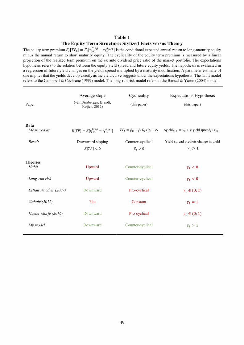
49
Table 1 The Equity Term Structure: Stylized Facts versus Theory
The equity term premium 𝐸𝑡[𝑇𝑃𝑡] = 𝐸𝑡[𝑟𝑡+1𝑙𝑜𝑛𝑔 − 𝑟𝑡+1
𝑠ℎ𝑜𝑟𝑡] is the conditional expected annual return to long-maturity equity minus the annual return to short maturity equity. The cyclicality of the equity term premium is measured by a linear projection of the realized term premium on the ex ante dividend price ratio of the market portfolio. The expectations hypothesis refers to the relation between the equity yield spread and future equity yields. The hypothesis is evaluated in a regression of future yield changes on the yields spread multiplied by a maturity modification. A parameter estimate of one implies that the yields develop exactly as the yield curve suggests under the expectations hypothesis. The habit model refers to the Campbell & Cochrane (1999) model. The long-run risk model refers to the Bansal & Yaron (2004) model.
Average slope Cyclicality Expectations Hypothesis
Paper (van Binsbergen, Brandt, Koijen, 2012) (this paper) (this paper)
Data
Measured as 𝐸[𝑇𝑃] = 𝐸[𝑟𝑡+1𝑙𝑜𝑛𝑔 − 𝑟𝑡+1
𝑠ℎ𝑜𝑟𝑡]
𝑇𝑃𝑡 = 𝛽0 + 𝛽1𝐷𝑡/𝑃𝑡 + 𝑒𝑡 Δyield𝑡+1 = 𝛾0 + 𝛾1yield spread𝑡+ϵ𝑡+1
Result Downward sloping
𝐸[𝑇𝑃] < 0
Counter-cyclical
𝛽1 > 0
Yield spread predicts change in yield
𝛾1 > 1
Theories
Habit Upward Counter-cyclical 𝛾1 < 0
Long-run risk Upward Counter-cyclical 𝛾1 < 0
Lettau Wacther (2007) Downward Pro-cyclical 𝛾1 ∈ (0; 1)
Gabaix (2012) Flat Constant 𝛾1 = 1
Hasler Marfe (2016) Downward Pro-cyclical 𝛾1 ∈ (0; 1)
My model Downward Counter-cyclical 𝛾1 > 1

50
Table 2 Counter-Cyclical Equity Term Premia
This table shows the relation between term premia and the dividend price ratio of the market portfolio. The table reports the parameter estimate from the following regression:
𝑟𝑡;𝑡+12𝑛 − 𝑟𝑡;𝑡+12
𝑚 = 𝛽0𝑛,𝑚 + 𝛽1
𝑛,𝑚(𝑑𝑡 − 𝑝𝑡) + 𝜖𝑡,𝑡+12
where 𝑑𝑡 − 𝑝𝑡 is the dividend price ratio of the market portfolio and 𝑟𝑡,𝑡+12𝑛 is the twelve-month forward return to the
dividend claim with n year maturity. The regression is based on monthly rolling regressions. The t-statistics are based on Newey and West (1987) standard errors corrected for 18 lags. The maturities n and m are both measured in years. The row m=mean(1-7) refers to the average return to the one- through seven-year maturity dividend claim. The sample is from 2005 to 2016.
Maturity of long-maturity claim (n)
2 3 4 5 6 7 Mkt
Panel A: S&P 500
m=1 0.12 0.18 0.25 0.34 0.41 0.45 0.59 (1.95) (2.61) (3.35) (3.97) (4.24) (4.50) (4.39)
m=2 0.05 0.12 0.21 0.26 0.29 0.35 (2.41) (3.64) (4.26) (4.19) (3.98) (2.40)
m=3 0.05 0.09 0.11 0.13 0.27 (1.96) (1.33) (1.21) (1.28) (1.99)
m=mean(1-7) 0.25 (1.89)
Panel B: Nikkei 225
m=1 0.40 0.69 0.77 0.81 0.84 0.87 0.75 (5.15) (3.54) (3.19) (2.92) (2.69) (2.57) (2.58)
m=2 0.21 0.30 0.36 0.40 0.43 0.39 (2.95) (2.61) (2.44) (2.27) (2.13) (1.83)
m=3 0.06 0.09 0.09 0.07 0.04 (1.46) (1.24) (0.94) (0.57) (0.28)
m=mean(1-7) 0.40 (0.52)
Panel C: EuroStoxx 50
m=1 0.23 0.39 0.41 0.40 0.39 0.36 0.37 (1.98) (2.63) (2.69) (2.76) (2.68) (2.39) (2.33)
m=2 0.07 0.07 0.05 0.02 0.01 0.03 (0.95) (0.67) (0.43) (0.23) (0.05) (0.22)
m=3 -0.03 -0.06 -0.09 -0.12 -0.05 (-1.13) (-1.51) (-1.89) (-2.32) (-0.49)
m=mean(1-7) 0.04 (0.41)
continued…

51
Panel D: FTSE 100
m=1 0.30 0.44 0.47 0.46 0.43 0.40 0.52 (2.61) (3.32) (3.69) (3.38) (2.92) (2.48) (2.34)
m=2 0.07 0.09 0.07 0.04 0.00 0.12 (1.12) (0.96) (0.61) (0.28) (0.01) (0.48)
m=3 0.01 -0.02 -0.06 -0.09 0.01 (0.15) (-0.32) (-0.64) (-0.87) (0.03)
m=mean(1-7) 0.09 (0.53)

52
Table 3 Counter-Cyclical Equity Term Premia: Excluding the Financial Crisis
This table shows the relation between term premia and the dividend price ratio of the market portfolio. The table reports the parameter estimate from the following regression:
𝑟𝑡;𝑡+12𝑛 − 𝑟𝑡;𝑡+12
𝑚 = 𝛽0𝑛,𝑚 + 𝛽1
𝑛,𝑚(𝑑𝑡 − 𝑝𝑡) + 𝜖𝑡,𝑡+12
where 𝑑𝑡 − 𝑝𝑡 is the dividend price ratio of the market portfolio and 𝑟𝑡,𝑡+12𝑛 is the twelve-month forward return to the
dividend claim with n year maturity. The regression is based on monthly rolling regressions. The t-statistics are based on Newey and West (1987) standard errors corrected for 18 lags. The maturities n and m are both measured in years. The row m=mean(1-7) refers to the average return to the one- through seven-year maturity dividend claim. The sample is from 2005 to 2016 excluding the years 2008 and 2009.
Maturity of long-maturity claim (n)
2 3 4 5 6 7 Mkt
Panel A: S&P 500
m=1 0.33 0.67 0.84 1.05 1.23 1.34 2.24 (4.24) (9.21) (9.42) (8.69) (8.25) (7.59) (3.60)
m=2 0.25 0.43 0.60 0.70 0.77 1.29 (3.70) (5.22) (5.46) (4.23) (3.66) (2.12)
m=3 0.06 0.03 0.03 0.07 0.82 (0.59) (0.13) (0.08) (0.19) (1.63)
m=mean(1-7) 0.97 (2.05)
Panel B: Nikkei 225
m=1 0.34 0.66 0.82 0.92 0.98 1.05 0.92 (10.24) (6.00) (5.05) (4.55) (4.16) (4.02) (2.17)
m=2 0.25 0.41 0.50 0.57 0.61 0.53 (5.00) (4.44) (4.23) (4.00) (3.74) (1.86)
m=3 0.10 0.15 0.16 0.15 0.06 (2.25) (1.90) (1.53) (1.08) (0.27)
m=mean(1-7) 0.05 (0.34)
Panel C: EuroStoxx 50
m=1 0.08 0.31 0.37 0.37 0.35 0.32 0.46 (1.20) (1.94) (2.20) (2.41) (2.30) (1.92) (1.99)
m=2 0.11 0.13 0.11 0.09 0.06 0.19 (1.30) (1.17) (0.89) (0.67) (0.45) (0.91)
m=3 -0.02 -0.05 -0.08 -0.12 0.05 (-0.39) (-0.75) (-1.03) (-1.41) (0.32)
m=mean(1-7) 0.15 (1.06)
Continued…

53
Panel D: FTSE 100
m=1 0.38 1.09 1.45 1.60 1.68 1.73 2.13 (4.02) (4.50) (5.94) (7.12) (8.26) (9.16) (5.99)
m=2 0.45 0.70 0.81 0.86 0.89 1.19 (2.34) (2.64) (2.76) (2.76) (2.80) (2.18)
m=3 0.20 0.28 0.31 0.34 0.57 (2.30) (2.10) (1.94) (1.95) (1.38)
m=mean(1-7) 0.56 (1.62)

54
Table 4 Counter-Cyclical Equity Term Premia: Using cay as Measure of Cyclicality
This table shows the relation between term premia and the ex ante value of cay (Lettau and Ludvigson, 2001). The table reports the parameter estimate from the following regression:
𝑟𝑡,𝑡+4𝑛 − 𝑟𝑡,𝑡+4
𝑚 = 𝛽0𝑛,𝑚 + 𝛽1
𝑛,𝑚cay𝑡 + 𝜖𝑡,𝑡+4
where 𝑟𝑡,𝑡+4𝑛 is the four-quarter forward return to the dividend claim with n year maturity. The regression is based on
quarterly rolling regressions. The t-statistics are based on Newey and West (1987) standard errors corrected for 6 lags. The maturities n and m are both measured in years. The row m=mean(1-7) refers to the average return to the one- through seven-year maturity dividend claim. The sample is from 2005 to 2016.
Maturity of long-maturity claim (n)
2 3 4 5 6 7 Mkt
Panel A: S&P 500
m=1 1.47 2.69 3.98 5.26 6.26 6.32 8.22 (1.25) (1.91) (2.76) (3.60) (4.20) (4.57) (4.36)
m=2 1.01 2.34 3.65 4.42 4.45 5.12 (2.27) (4.55) (5.29) (5.31) (3.89) (2.73)
m=3 1.28 2.47 3.19 3.20 4.08 (4.92) (3.82) (3.63) (2.74) (2.30)
m=mean(1-7) 2.96 (1.54)
Panel B: S&P 500 (excluding 2008-2009)
m=1 2.94 5.00 6.27 7.55 8.53 8.15 9.47 (3.06) (5.53) (6.36) (6.09) (5.52) (4.32) (4.31)
m=2 1.78 3.07 4.41 5.12 4.75 4.78 (3.35) (4.33) (4.01) (3.56) (2.38) (1.92)
m=3 1.32 2.72 3.46 3.10 3.10 (3.99) (2.72) (2.48) (1.66) (1.34)
m=mean(1-7) 2.28 (0.89)

55
Table 5 Counter-Cyclical Sharpe Ratios
This table shows the relation between the sharpe ratios for term premia and the dividend price ratio of the market portfolio. The table reports the parameter estimate from the following regression:
𝑆𝑅𝑡;𝑡+12𝑛,𝑚 = 𝛽0
𝑛,𝑚 + 𝛽1𝑛,𝑚(𝑑𝑡 − 𝑝𝑡) + 𝜖𝑡,𝑡+12
where 𝑑𝑡 − 𝑝𝑡 is the dividend price ratio of the market portfolio and 𝑆𝑅𝑡,𝑡+12𝑛,𝑚 is the one-year log-Sharpe ratio of the log-
return to the n maturity claim minus the return to the m maturity claim. The regression is based on monthly rolling regressions. The t-statistics are based on Newey and West (1987) standard errors corrected for 18 lags. The maturities n and m are both measured in years. The sample is from 2005 to 2016.
Maturity of long-maturity claim (n)
2 3 4 5 6 7 Mkt
Panel A: S&P 500
m=1 3.18 3.27 3.70 4.19 4.15 3.74 3.43 (2.84) (3.44) (4.47) (5.43) (5.58) (5.79) (6.69)
m=2 1.54 2.87 3.67 3.67 3.10 1.78 (2.65) (5.27) (6.60) (5.51) (6.19) (2.61)
m=3 2.17 2.13 1.83 1.46 1.40 (3.10) (2.20) (1.54) (1.52) (2.11)
m=mean(1-7) 1.57 (2.16)
Panel B: Nikkei 225
m=1 5.28 5.43 5.91 6.04 5.79 5.41 4.65 (6.91) (5.88) (5.35) (4.84) (4.34) (3.91) (2.81)
m=2 3.66 4.31 4.34 4.02 3.59 2.48 (3.55) (3.03) (2.74) (2.43) (2.12) (1.77)
m=3 2.89 2.48 2.00 1.46 0.50 (1.63) (1.41) (1.19) (0.88) (0.60)
m=mean(1-7) 0.71 (1.09)
Panel C: EuroStoxx 50
m=1 1.92 2.38 2.61 2.54 2.64 2.46 2.00 (2.42) (2.45) (2.64) (2.59) (2.78) (2.70) (2.89)
m=2 1.52 0.92 0.48 0.63 0.55 0.50 (1.18) (0.93) (0.53) (0.62) (0.57) (0.63)
m=3 -0.68 -0.93 -0.76 -0.74 0.35 (-0.79) (-1.09) (-0.85) (-0.87) (0.58)
m=mean(1-7) 1.06 (1.72)
Continued…

56
Panel D: FTSE 100
m=1 4.02 4.32 4.64 4.60 4.43 4.12 3.20 (3.81) (3.80) (3.81) (3.88) (4.03) (3.83) (3.85)
m=2 2.17 2.11 1.75 1.57 1.25 0.88 (1.47) (1.27) (1.01) (0.99) (0.78) (0.74) m=3 0.57 0.17 -0.05 -0.30 0.22 (0.38) (0.11) (-0.04) (-0.22) (0.24) m=mean(1-7) 0.77 (0.99)

57
Table 6 Counter-Cyclical Equity Term Premia: Alternative Measures
This table shows the relation between term premia and the dividend price ratio of the market portfolio. The term premia are measured in two different ways: (1) as the implied term premium from equity options (van Binsbergen, Brandt, and Koijen, 2012) and (2) as the return to a term premium mimicking portfolio from the cross-section of equities. The term premium mimicking portfolio is long a portfolio with long duration firms and short a portfolio with short duration firms. To construct the long and short duration portfolios, I run a regression of the excess return to 30 portfolios sorted on book-to-market, profitability, and investment onto the realized return difference between long- and short-maturity equity claims between 1996 and 2015. For each style, I rank portfolios in ascending order based on their beta with respect to long- minus short-maturity return difference. I assign the two portfolios with highest (lowest) beta to the long (short) duration portfolio. Within the long (short) duration portfolio I equal weight the excess return. I include as independent variables the ex ante dividend price ratio of the market portfolio, the five Fama and French (20015) factors, the ex ante one-year treasury yield, and the ex ante treasury yield spread (five-year yield in excess of one-year yield). The yields are from Fama and Bliss (1987). All returns are measured in rolling one-year log returns. I report t-statistics below the parameter estimates. The t-statistics are based on Newey and West (1987) standard errors corrected for 18 lags. The results are from the U.S.
Panel A: Alternative measures of the equity term premium
Option implied term premium Cross-sectional term premium
Period 1996-2009 1996-2009 1963-2015 1963-2015 1996-2015 1963-1996 dt - pt 1.04 0.90 0.04 0.07 0.13 0.07 (2.55) (5.93) (0.92) (3.68) (1.54) (1.68)
Mkt 0.30 0.10 -0.03 0.11 (0.91) (3.23) (-0.51) (3.09)
SMB -0.65 0.25 0.23 0.25 (-2.41) (7.09) (2.85) (4.83) HML -0.45 -0.34 -0.20 -0.38 (-1.32) (-7.41) (-3.14) (-7.03) RMW -0.79 -0.59 -0.89 -0.43 (-1.44) (-9.24) (-9.46) (-5.01) CMA 0.26 -0.09 -0.03 -0.05 (0.55) (-1.13) (-0.20) (-0.51) Bond yield 0.05 -0.01 0.00 -0.01 (1.31) (-2.92) (-0.19) (-3.76) Bond yield spread 0.10 -0.02 -0.01 -0.02 (1.28) (-3.40) (-0.86) (-3.00)

58
Panel B: Alternative measures of cyclicality
Option implied term premium Cross-sectional term premium Period 1996-2009 1996-2009 1996-2009 1996-2009 1963-2015 1963-2015 CAPEt 0.59 0.96 0.05 (1.46) (5.17) (2.42) cayt 3.07 -2.78 0.81 (0.61) (-0.61) (1.99) Mkt 0.30 0.98 0.10 0.10 (0.88) (1.78) (3.02) (3.28) SMB -0.73 -1.14 0.26 0.18 (-2.51) (-1.64) (7.09) (2.37) HML -0.64 -0.81 -0.32 -0.13 (-2.35) (-1.50) (-6.48) (-1.12)
RMW -0.77 0.22 -0.62 -0.08 (-1.43) (0.48) (-9.66) (-0.55) CMA 0.15 0.69 -0.15 0.13 (0.37) (0.55) (-1.74) (0.72) Bond yield 0.11 -0.03 -0.01 0.00 (2.11) (-0.52) (-2.01) (-0.96) Bond yield spread 0.13 0.04 -0.02 -0.02 (1.39) (0.33) (-3.09) (-1.74)

59
Table 7 The Expectations Hypothesis: The Yield Spread and Long-Yield Changes
This table shows the relation between long-yield changes and the equity yield spread. The table reports the parameter estimate from the following regression:
𝑒𝑡+𝑚𝑛−𝑚 − 𝑒𝑡
𝑛 = 𝛾0𝑛,𝑚 + 𝛾1
𝑛,𝑚𝑠𝑡𝑛,𝑚 𝑚
𝑛 − 𝑚+ 𝜖𝑡+𝑚
The expectations hypothesis is that 𝛾1𝑛,𝑚 = 1 for all maturity pairs n,m. The t-statistics for this hypothesis are reported
below the parameter estimates. The t-statistics are based on Newey and West (1987) standard errors corrected for 1.5m lags. The maturities n and m are both measured in years. The sample is from 2005 to 2016.
Maturity of long-maturity claim (n)
2 3 4 5 6 7
Panel A: S&P 500
m=1 1.00 1.08 1.18 1.27 1.36 1.38 (-0.00) (0.17) (0.46) (0.70) (0.93) (1.07)
m=2 1.61 1.77 1.87 1.95 2.04 (2.08) (2.16) (2.51) (2.91) (3.32)
m=3 1.73 1.94 2.09 2.15 (3.04) (3.25) (3.09) (3.29)
Panel B: Nikkei 225
m=1 1.62 1.59 1.30 1.17 1.07 0.99 (1.02) (0.92) (0.53) (0.32) (0.14) (-0.02)
m=2 1.05 0.97 0.85 0.79 0.74 (0.11) (-0.07) (-0.33) (-0.46) (-0.59)
m=3 1.23 1.29 1.19 1.14 (0.34) (0.37) (0.26) (0.19)
Panel C: EuroStoxx 50
m=1 2.72 3.86 3.10 2.79 2.62 2.53 (2.03) (5.37) (5.91) (5.92) (5.76) (5.58)
m=2 1.61 1.58 1.46 1.36 1.33 (2.80) (2.05) (1.78) (1.59) (1.52)
m=3 1.04 1.13 1.01 0.93 (0.09) (0.25) (0.03) (-0.19)
Panel D: FTSE 100
m=1 -1.20 1.71 2.04 2.03 1.96 1.88 (-3.50) (0.85) (1.55) (2.05) (2.41) (2.56)
m=2 1.56 1.71 1.59 1.52 1.47 (1.90) (1.74) (1.70) (1.68) (1.66)
m=3 1.26 1.19 1.03 0.95 (1.06) (0.58) (0.10) (-0.17)

60
Table 8 The Expectations Hypothesis: The Yield Spread and Short-Yield Changes
This table shows the relation between short-yield changes and the equity yield spread. The table reports the parameter estimate from the following regression:
∑ (1 −𝑖𝑛
) (𝑒𝑡+𝑚𝑚 − 𝑒𝑡+(𝑖−1)𝑚
𝑚 )𝑘−1
𝑖=1
= 𝜙𝑜𝑛,𝑚 + 𝜙1
𝑛,𝑚𝑠𝑡𝑛,𝑚 + 𝜂𝑡+𝑛
The expectations hypothesis is that 𝜙1𝑛,𝑚 = 1 for all maturity pairs n,m. The t-statistics for this hypothesis are reported
below the parameter estimates. The t-statistics are based on Newey and West (1987) standard errors corrected for 1.5m lags. The maturities n and m are both measured in years. The sample is from 2005 to 2016.
Maturity of long-maturity claim (n)
2 3 4 5 6
Panel A: S&P 500
m=1 1.00 1.23 1.23 1.25 1.26 (-0.00) (1.41) (1.98) (2.58) (2.02)
m=2 1.38 1.37 (2.24) (3.60)
Panel B: Nikkei 225
m=1 1.31 1.15 0.98 1.06 1.07 (0.92) (0.70) (-0.10) (0.35) (0.37)
m=2 0.98 1.13 (-0.07) (0.63)
Panel C: EuroStoxx 50
m=1 1.86 2.07 1.49 1.30 0.72 (3.07) (6.18) (3.81) (3.55) (-3.82)
m=2 1.29 1.12 (2.66) (2.09)
Panel D: FTSE 100
m=1 -0.10 1.43 1.37 1.34 1.17 (-4.58) (1.45) (1.84) (2.68) (1.69)
m=2 1.36 1.20 (1.79) (2.07)

61
Table 9 Cyclicality of the Investment Duration
This table reports the results from a regression of investment characteristics on the dividend price ratio of the market portfolio plus controls. I consider the investment rates for three portfolios: a portfolio with short-duration firms, a portfolio with long-duration firms, and a long/short portfolio. To construct the long- and short-duration portfolio, I run a regression of the excess return to 30 portfolios sorted on book-to-market, profitability, and investment onto the realized return difference between long- and short-maturity equity claims between 1996 and 2015. For each style, I rank portfolios in ascending order based on their beta with respect to long- minus short-maturity return difference. I assign the two portfolios with highest (lowest) beta to the long (short) duration portfolio. Within the long (short) duration portfolio I equal-weight the characteristics. Capital to labor is measured as capital expenditures to total salary. Investment is measured as capital expenditure to plant, property, and equipment. Change in Capex is the change in capital expenditure. R&D is the annual change in salary spend on R&D activities. Total salary expenses is the annual change in total salaries. All characteristics are measured in cross-sectional percentiles. In the regressions, I use as the independent variables the ex ante dividend price ratio of the market portfolio, the one-year treasury yield, the treasury yield spread (five-year in excess of one-year), and a dummy variable for NBER recessions. I report t-statistics below the parameter estimates. The t-statistics are based on Newey and West (1987) standard errors corrected for 18 lags. The sample is U.S. equities from 1963-2015.
Panel A: Capital to labor
Portfolio Short duration
Long duration Long- minus short duration
Period 1963-2015 1963-2015 1963-2015 1963-2015 1996-2015 1963-1996 dt - pt 2.85 -4.03 -6.88 -6.86 -0.54 -4.08 (10.93) (-9.09) (-10.56) (-5.50) (-2.64) (-1.76) Bond yieldt 0.01 -0.31 0.38 (0.04) (-8.99) (1.96) Bond yield spreadt 0.91 -0.57 1.38 (1.52) (-4.27) (2.92) Recession dummyt 1.35 0.22 0.20 (1.70) (1.74) (0.23)
Panel B: Detrended capital to labor
Capital to labor (HP filter) Capital to labor (first difference)
Portfolio Long-short Long-short Long-short Long-short Long-short Long-short Period 1963-2015 1996-2015 1963-2015 1963-2015 1996-2015 1963-1996
dt - pt (HP filter) -2.00 -0.45 -3.78 (-2.02) (-1.70) (-1.92) dt - pt (first differenced) -1.14 -0.97 -1.33 (-0.95) (-2.18) (-0.60) Bond yieldt 0.02 -0.08 0.03 0.05 -0.04 0.14 (0.67) (-1.58) (0.39) (1.36) (-0.62) (1.47) Bond yield spreadt -0.16 -0.26 -0.26 0.10 -0.24 0.21 (-0.93) (-1.63) (-1.12) (0.49) (-1.60) (0.73) Recession dummyt 0.35 -0.01 0.51 0.21 0.21 0.11 (1.13) (-0.03) (1.16) (0.44) (0.83) (0.16)

62
Panel C: Investment
Investment measure Investment (Capex to PPE) Change in CapEx
Portfolio Short duration
Long duration Long-short Short
duration Long
duration Long-short
Period 1963-2015 1963-2015 1963-2015 1963-2015 1963-2015 1963-2015 dt - pt 1.84 -3.48 -9.13 2.54 -4.17 -10.14 (3.27) (-4.13) (-4.16) (4.86) (-4.85) (-4.51)
Bond yieldt 0.74 0.66 (2.12) (1.91)
Bond yield spreadt 1.68 1.10 (1.87) (1.11)
Recession dummyt 2.58 1.90 (2.64) (1.57)
Panel D: R&D and Salary
Characteristic: R&D Total Salary Expenses
Portfolio Short duration
Long duration Long-short Short
duration Long
duration Long-short
Period 1963-2015 1963-2015 1963-2015 1963-2015 1963-2015 1963-2015 dt - pt 2.74 -5.85 -9.26 0.07 0.83 0.82 (6.37) (-9.96) (-6.12) (0.22) (2.15) (1.21) Bond yieldt 0.10 0.06 (0.40) (0.53) Bond yield spreadt 0.67 0.77 (1.01) (2.60) Recession dummyt 1.88 -0.38 (1.77) (-0.75)

63
Table 10 Asset Pricing Theories versus Stylized Facts
This table shows the result of simulations of different asset pricing models. I simulate the models and estimate the following regressions:
𝑟𝑡;𝑡+12𝑛 − 𝑟𝑡;𝑡+12
𝑚 = 𝛽0𝑛,𝑚 + 𝛽1
𝑛,𝑚(𝑑𝑡 − 𝑝𝑡) + 𝜖𝑡,𝑡+12
𝑒𝑡+𝑚𝑛−𝑚 − 𝑒𝑡
𝑛 = 𝛾0𝑛,𝑚 + 𝛾1
𝑛,𝑚𝑠𝑡𝑛,𝑚 𝑚
𝑛 − 𝑚+ 𝜖𝑡+𝑚
∑ (1 −𝑖𝑛
) (𝑒𝑡+𝑚𝑚 − 𝑒𝑡+(𝑖−1)𝑚
𝑚 )𝑘−1
𝑖=1
= 𝜙𝑜𝑛,𝑚 + 𝜙1
𝑛,𝑚𝑠𝑡𝑛,𝑚 + 𝜂𝑡+𝑛
where 𝑟𝑡+12𝑛 is the forward log-return on the n maturity claim between month t and t+12, 𝑑𝑡 − 𝑝𝑡 is the log dividend price
ratio of the market portfolio, 𝑒𝑡𝑛 is the yield on the n maturity dividend at time t, and 𝑦𝑡
𝑛,𝑚 is the yield spread between the n and the m maturity dividend at time t. Maturities n and m are measured in years. The habit model is the Campbell and Cochrane (1999) model. The model is simulated using the series method of Wachter (2005). The long-run risk model is the model by Bansal and Yaron (2004) that features stochastic volatility.
𝐸[𝑟𝑡+12𝑚𝑘𝑡 − 𝑟𝑡+12
2 ] 𝛽1𝑚𝑘𝑡,2 𝛾1
5,1 𝜙15,1
Data
Empirical observation -0.035 0.35 1.27 1.25
Theories
Habit 0.038 0.12 -1.32 -0.80
Long-run risk 0.029 0.03 -0.95 -0.03
Lettau & Wacther (2007) -0.067 -0.08 0.32 0.72
Disaster (Gabaix, 2012) 0 0 1 1
My model
-0.01 0.10 2.4 1.6

64
Table 11 Reconciling Theory with the Empirical Facts: Simulated Results in an Asset Pricing Model
This table shows results of simulations in my model. The results are based on 100,000 years of artificial data. The model is simulated to fit the U.S. data in the 1996-2016 period. The model is simulated on the quarterly horizon. Expected returns and standard deviations are annualized (multiplied by 4 and 2).
Data Model
Stock market moments
𝐸[𝑅𝑡+1𝑚 − 𝑅𝑓] 0.07 0.07
𝜎[𝑅𝑡+1𝑚 − 𝑅𝑓] 0.18 0.23
𝐸[𝑃𝑡/𝐷𝑡] 57.3 49.7
𝜎(𝑝𝑡 − 𝑑𝑡) 0.22 0.28
AR1(𝑝𝑡 − 𝑑𝑡) 0.92 0.90
Term structure of equity results
𝐸[𝑟𝑡+12𝑚𝑘𝑡 − 𝑟𝑡+12
2 ] -0.035 -0.01
𝛽1𝑚𝑘𝑡,2 0.35 0.10
𝛾15,1 1.27 2.4
𝜙15,1 1.25 1.6

65
Figure 1 The Term Structure of One-Year Equity Returns
This figure shows the term structure of holding-period equity returns for the S&P 500. The figure shows the unconditional average return (solid line), the average return in bad times (dashed line), and the average return in good times (dash-dotted line). Good and bad times are defined by the ex ante dividend price ratio. Short-maturity equity claims is the average return to dividend futures of 1 to 7 years maturity. The long-maturity claim is the average return to the market portfolio. Returns are annual spot returns, 2005 – 2016.
-0.02
0.00
0.02
0.04
0.06
0.08
0.10
0.12
0.14
0.16
Short-maturity claims Long-maturity claims
Annual return
Average Bad times Good times

66
Figure 2 The Equity Term Structure in Good and Bad Times
This figure shows the term structure of one-year equity returns in good and bad times. Panel A shows the equity term structure estimated using dividend futures. The short-maturity return is the return to the one- and two-year dividend claims and the long-maturity return is the return to the six- and seven-year claims – all measured in excess of the cross-sectional and time-series averages. Panel B shows the equity term structure estimated using option implied dividends. The short-maturity claim is the return to the two-year dividend and the long-maturity claim is the return to the market portfolio, measured in excess of the cross-sectional and time-series averages. Panel C shows the term structure estimated using the cross-section of stocks. The duration of stocks is measured by a regression of excess returns on the realized long- minus short-maturity return in the 1996-2016 sample. Returns are measured as annual alpha in the five-factor model. Good (bad) times are months where the dividend price ratio is below (above) the median.
Panel A: Estimated using dividend futures (2005-2016)
Panel B: Estimated using option implied dividend prices (1996-2009)
Panel C: Estimated using the cross-section of stocks (1963-2015)
-4
-2
0
2
4
6
Short duration Long Duration
Bad times
-6
-4
-2
0
2
4
6
Short duration Long DurationFutu
res r
etur
n in
exc
ess o
f th
e av
erag
e (a
nnua
l per
cent
)
Good times
-8-6-4-202468
Short maturity Long maturity
Ret
urn
in e
xces
s of t
he
aver
age
(ann
ual p
erce
nt)
Good times
-8-6-4-202468
Short maturity Long maturity
Bad times
-0.7-0.6-0.5-0.4-0.3-0.2-0.1
00.10.2
Short duration firms Long duration firms
Bad times
-1
-0.5
0
0.5
1
1.5
Short duration firms Long duration firms
Ann
ual a
lpha
Good times

67
Figure 3 Real Effects of the Equity Term Structure
This figure shows average firm characteristics in good and bad times for firms with different duration of cash flows. Panel A shows the investment rate measured as CAPEX over the value of property, plant, and equipment. Panel B shows the annual change in capital expenditure. Panel C shows the capital to labor ratio measured as CAPEX to salaries. All characteristics are measured as cross-sectional percentiles in excess of the given portfolios time-series average. Duration is measured by sensitivity to the equity term premium. Good (bad) times are months where the dividend price ratio is below (above) the median. The sample is from 1964-2015.
Panel A: Investment (CAPEX/PPE)
Panel B: Investment (increase in capital expenditure)
Panel C: Capital to Labor Ratio
-0.3
-0.2
-0.1
0
0.1
0.2
0.3
Short duration firms Long duration firms
Inve
stm
ent r
ate
Good times
-0.3
-0.2
-0.1
0
0.1
0.2
0.3
Short duration firms Long duration firms
Bad times
-0.2
-0.1
0
0.1
0.2
0.3
0.4
0.5
Short duration firms Long duration firms
Incr
ease
in C
apEx
Good times
-0.5
-0.4
-0.3
-0.2
-0.1
0
0.1
0.2
Short duration firms Long duration firms
Bad times
-1.5
-1
-0.5
0
0.5
1
1.5
2
Short duration firms Long duration firms
Cap
ital t
o La
bor r
atio
Good times
-2
-1.5
-1
-0.5
0
0.5
1
1.5
Short duration firms Long duration firms
Bad times

68
Figure 4 Realized Long-minus-Short Return and Dividend Price Ratios
This figure shows, for four different indexes, the ex ante log dividend price ratio and the realized return difference between long- and short-maturity claims. The future long-minus-short return is the average two-year log-return to the six- and seven-year dividend claim minus the average two-year log-return to the one- and two-year dividend claim. The graph indicates the starting date of the two-year period. After 2005 returns are based on dividend futures. Before 2005, the U.S. term premium is the two-year return difference between the two- and the one-year option implied dividend returns.
-4.8-4.6-4.4-4.2-4-3.8-3.6-3.4-3.2
-0.8-0.6-0.4-0.2
00.20.40.60.8
01-1
996
06-1
997
11-1
998
04-2
000
09-2
001
02-2
003
07-2
004
12-2
005
05-2
007
10-2
008
03-2
010
08-2
011
01-2
013
06-2
014
Div
iden
pric
e ra
tio
Ret
urn
S&P 500
Future long-minus-short return
Dividend price ratio
-5-4.8-4.6-4.4-4.2-4-3.8-3.6
-1.2-1
-0.8-0.6-0.4-0.2
00.20.40.60.8
02-2
005
11-2
005
08-2
006
05-2
007
02-2
008
11-2
008
08-2
009
05-2
010
02-2
011
11-2
011
08-2
012
05-2
013
02-2
014
11-2
014
Div
iden
pric
e ra
tio
Ret
urn
Nikkei 225
Future long-minus-short return
Dividend price ratio
-3.9-3.7-3.5-3.3-3.1-2.9-2.7-2.5
-1-0.8-0.6-0.4-0.2
00.20.4
01-2
006
09-2
006
05-2
007
01-2
008
09-2
008
05-2
009
01-2
010
09-2
010
05-2
011
01-2
012
09-2
012
05-2
013
01-2
014
09-2
014
Div
iden
pric
e ra
tio
Ret
urn
Euro Stoxx 50
Future long-minus-short return
Dividend price ratio
-3.8
-3.6
-3.4
-3.2
-3
-2.8
-1.3
-0.8
-0.3
0.2
0.7
1.2
01-2
006
09-2
006
05-2
007
01-2
008
09-2
008
05-2
009
01-2
010
09-2
010
05-2
011
01-2
012
09-2
012
05-2
013
01-2
014
09-2
014
Div
iden
pric
e ra
tio
Ret
urn
FTSE 100
Future long-minus-short return
Dividend price ratio

69
Figure 5 Realized Long-minus-Short Return
This figure shows for four different indexes the ex ante value of the cay variable and the realized return difference between long- and short-maturity claims. The future long-minus-short return is the average two-year log-return to the six- and seven-year dividend claim minus the average two-year log-return to the one- and two-year dividend claim. The graph indicates the starting date of the two-year period. After 2005 returns are based on dividend futures. Before 2005, the U.S. term premium is the two-year return difference between the two- and the one-year option implied dividend returns. The figure shows the U.S. cay variable for all indexes.
-0.04-0.03-0.02-0.010.000.010.020.030.04
-0.6
-0.4
-0.2
0
0.2
0.4
0.6
01-1
996
06-1
997
11-1
998
04-2
000
09-2
001
02-2
003
07-2
004
12-2
005
05-2
007
10-2
008
03-2
010
08-2
011
01-2
013
06-2
014
CA
Y
Ret
urn
S&P 500
Future long-minus-short return CAY
-0.04
-0.03
-0.02
-0.01
0.00
0.01
0.02
-1.20-1.00-0.80-0.60-0.40-0.200.000.200.400.600.80
01-2
006
09-2
006
05-2
007
01-2
008
09-2
008
05-2
009
01-2
010
09-2
010
05-2
011
01-2
012
09-2
012
05-2
013
01-2
014
09-2
014
CA
Y
Ret
urn
Nikkei 225
Future long-minus-short return CAY
-0.04
-0.03
-0.02
-0.01
0.00
0.01
0.02
-1.00
-0.80
-0.60
-0.40
-0.20
0.00
0.20
0.40
01-2
006
09-2
006
05-2
007
01-2
008
09-2
008
05-2
009
01-2
010
09-2
010
05-2
011
01-2
012
09-2
012
05-2
013
01-2
014
09-2
014
CA
Y
Ret
urn
Euro Stoxx 50
Future long-minus-short return CAY
-0.04
-0.03
-0.02
-0.01
0.00
0.01
0.02
-1.00-0.80-0.60-0.40-0.200.000.200.400.60
01-2
006
09-2
006
05-2
007
01-2
008
09-2
008
05-2
009
01-2
010
09-2
010
05-2
011
01-2
012
09-2
012
05-2
013
01-2
014
09-2
014
CA
Y
Ret
urn
FTSE 100
Future long-minus-short return CAY

70
Figure 6 Time Variation in The Term Structure of Equity Yields
This figure shows the time variation in the term structure of equity yields. The figure shows the yield for the two-, five-, and seven-year dividend claim. The equity yield for dividends that are paid out at time t+n are defined as:
where 𝑑𝑡 is the rolling annual dividends at time t and 𝑓𝑡𝑛 is the forward price of the n maturity claim at time t.
-0.2
-0.1
0
0.1
0.2
0.3
0.4
0.5
0.6
01-2
005
10-2
005
07-2
006
04-2
007
01-2
008
10-2
008
07-2
009
04-2
010
01-2
011
10-2
011
07-2
012
04-2
013
01-2
014
10-2
014
07-2
015
Nikkei 225
2 year yield
5 year yield
7 year yield
-0.2-0.15-0.1
-0.050
0.050.1
0.150.2
0.250.3
01-2
005
01-2
006
01-2
007
01-2
008
01-2
009
01-2
010
01-2
011
01-2
012
01-2
013
01-2
014
01-2
015
01-2
016
Equity yield
S&P 500
2 year yield
5 year yield
7 year yield
-0.2
-0.1
0
0.1
0.2
0.3
0.4
0.5
01-2
005
10-2
005
07-2
006
04-2
007
01-2
008
10-2
008
07-2
009
04-2
010
01-2
011
10-2
011
07-2
012
04-2
013
01-2
014
10-2
014
07-2
015
FTSE 100
2 year yield
5 year yield
7 year yield
-0.3-0.2-0.1
00.10.20.30.40.50.6
01-2
005
10-2
005
07-2
006
04-2
007
01-2
008
10-2
008
07-2
009
04-2
010
01-2
011
10-2
011
07-2
012
04-2
013
01-2
014
10-2
014
07-2
015
Equity yield
EuroStoxx 50
2 year yield
5 year yield
7 year yield

71
Figure 7 Reconciling the Facts in an Asset Pricing Model: Equity Term Premia in Good and Bad
Times This figure shows equity term premia 𝜃𝑡
𝑛,1 in the asset pricing model on average, in good times, and in bad times. The term premia are plotted as a function of the long-maturity claims (the x-axis). Good (bad) times are periods where the ex ante dividend price ratio of the market portfolio is below (above) the time series median. The results are based on 100,000 years of artificial quarterly data.
-0.05
-0.04
-0.03
-0.02
-0.01
0.00
0.01
0.02
0.03
1 5 9 13 17 21 25 29 33 37 41 45 49
Ann
ualiz
ed T
erm
Pre
miu
m
Horizon (quarters)
Average Average good times Average bad times

72
Table A1 Summary Statistics on Dividend Futures
This table provides summary statistics for dividend futures. Returns and standard deviations are for annualized claims. The loading on the dividend price ratio refers to the regression coefficient in a regression of realized excess returns on the ex ante log dividend price ratio of the market portfolio. Good and bad times are based on the median dividend price ratio.
Maturity of dividend claim (years)
1 2 3 4 5 6 7 Mkt
Panel A: S&P 500
Average futures returns 0.015 0.012 0.021 0.021 0.024 0.028 0.037 -0.024 Variance annual returns 0.002 0.017 0.027 0.031 0.038 0.044 0.048 0.077 Variance quarterly returns 0.006 0.023 0.025 0.030 0.037 0.041 0.046 0.080 Loading on dt − pt 0.059 0.275 0.328 0.404 0.489 0.548 0.575 0.677 Average good times 0.017 -0.006 0.010 0.002 0.000 0.000 0.012 -0.080 Average bad times 0.013 0.029 0.034 0.045 0.053 0.062 0.067 0.041 Average yields -0.038 -0.044 -0.044 -0.042 -0.041 -0.038 -0.035 Standard dev. of yield 0.115 0.077 0.052 0.042 0.036 0.033 0.029
Panel B: Nikkei 225
Average futures returns 0.109 0.071 0.048 0.077 0.081 0.084 0.089 -0.040 Variance annual returns 0.006 0.071 0.117 0.135 0.150 0.161 0.170 0.121 Variance quarterly returns 0.018 0.084 0.107 0.113 0.119 0.121 0.123 0.117 Loading on dt − pt 0.088 0.611 0.855 0.953 1.015 1.055 1.086 1.002 Average good times 0.055 -0.051 -0.083 -0.011 -0.004 0.004 0.017 -0.097 Average bad times 0.13 0.15 0.16 0.16 0.17 0.16 0.16 0.02 Average yields 0.020 0.004 -0.013 -0.017 -0.016 -0.014 -0.012 Standard dev. of yield 0.160 0.131 0.097 0.077 0.065 0.056 0.048
Panel C: Euro Stoxx 50
Average futures returns 0.033 0.044 0.019 0.004 -0.003 -0.007 -0.007 -0.062 Variance annual returns 0.005 0.044 0.091 0.100 0.100 0.099 0.099 0.099 Variance quarterly returns 0.010 0.063 0.080 0.083 0.084 0.082 0.084 0.090 Loading on dt − pt 0.096 0.500 0.605 0.604 0.587 0.570 0.549 0.560 Average good times -0.004 -0.015 -0.035 -0.047 -0.050 -0.050 -0.045 -0.120 Average bad times 0.033 0.126 0.110 0.089 0.075 0.064 0.056 0.035 Average yields 0.056 0.046 0.031 0.025 0.020 0.015 0.012
Standard dev. of yield 0.128 0.124 0.086 0.066 0.053 0.045 0.038
Panel D: FTSE 100
Average futures returns 0.018 0.038 0.027 0.020 0.017 0.017 0.020 -0.035 Variance annual returns 0.005 0.030 0.064 0.072 0.073 0.071 0.070 0.063 Variance quarterly returns 0.009 0.043 0.054 0.058 0.059 0.060 0.061 0.062 Loading on dt − pt 0.151 0.763 0.853 0.876 0.854 0.823 0.787 0.917 Average good times -0.012 -0.018 -0.013 -0.023 -0.026 -0.023 -0.018 -0.089 Average bad times 0.069 0.089 0.071 0.069 0.065 0.063 0.064 0.025 Average yields 0.000 0.005 0.001 0.000 -0.002 -0.002 -0.002
Standard dev. of yield 0.098 0.099 0.069 0.053 0.042 0.035 0.030

73
Table A2 Counter-Cyclical Equity Term Premia: Quarterly Returns
This table shows the relation between term premia and the dividend price ratio of the market portfolio. The table reports the parameter estimate from the following regression:
𝑟𝑡;𝑡+3𝑛 − 𝑟𝑡;𝑡+3
𝑚 = 𝛽0𝑛,𝑚 + 𝛽1
𝑛,𝑚(𝑑𝑡 − 𝑝𝑡) + 𝜖𝑡,𝑡+3
where 𝑑𝑡 − 𝑝𝑡 is the dividend price ratio of the market portfolio and 𝑟𝑡,𝑡+3𝑛 is the three-month forward return to the dividend
claim with n year maturity. The regression is based on monthly rolling regressions. The t-statistics are based on Newey and West (1987) standard errors corrected for 8 lags. The maturities n and m are both measured in years. The row m=mean(1-7) refers to the average return to the one- through seven-year maturity dividend claim. The sample is from 2005 to 2016.
Maturity of long-maturity claim (n)
2 3 4 5 6 7 Mkt
Panel A: S&P 500
m=1 0.03 0.06 0.09 0.12 0.13 0.15 0.23 (0.50) (1.07) (1.63) (1.91) (2.00) (2.09) (3.23)
m=2 0.01 0.04 0.06 0.07 0.07 0.08 (1.33) (2.66) (2.57) (2.29) (2.06) (1.03)
m=3 0.02 0.02 0.03 0.04 0.08 (1.13) (0.84) (1.15) (1.03) (1.22)
m=mean(1-7) 0.08 (1.18)
Panel B: Nikkei 225
m=1 0.13 0.17 0.16 0.18 0.19 0.20 0.23 (2.33) (2.27) (2.07) (2.17) (2.15) (2.30) (1.31)
m=2 0.01 0.02 0.04 0.04 0.05 0.16 (0.49) (0.72) (0.96) (0.95) (0.97) (1.39)
m=3 0.00 0.01 0.01 0.00 0.06 (0.53) (0.56) (0.30) (-0.05) (0.68)
m=mean(1-7) 1.20 (0.19)
Panel C: EuroStoxx 50
m=1 0.09 0.07 0.06 0.04 0.03 0.03 0.04 (1.08) (0.75) (0.65) (0.49) (0.41) (0.31) (0.37)
m=2 -0.03 -0.04 -0.05 -0.06 -0.06 -0.02 (-1.33) (-1.50) (-1.65) (-2.18) (-2.36) (-0.59)
m=3 -0.01 -0.02 -0.03 -0.03 0.02 (-1.69) (-1.38) (-1.55) (-1.63) (0.38)
m=mean(1-7) 0.03 (0.90)
continued…

74
Panel D: FTSE 100
m=1 0.18 0.16 0.17 0.17 0.17 0.16 0.19 (1.62) (1.29) (1.48) (1.51) (1.65) (1.59) (2.02)
m=2 -0.06 -0.07 -0.08 -0.08 -0.08 0.00 (-1.48) (-1.42) (-1.50) (-1.31) (-1.33) (-0.04)
m=3 -0.01 -0.02 -0.02 -0.03 0.06 (-0.84) (-0.99) (-0.63) (-0.66) (0.66)
m=mean(1-7) 0.08 (1.17)

75
Table A3 Counter-Cyclical Difference in Sharpe Ratios
This table shows the relation between the difference in Sharpe ratios for equity claims with different maturity and the dividend price ratio of the market portfolio. The table reports the parameter estimate from the following regression:
𝑆𝑅𝑡,𝑡+12𝑛 − 𝑆𝑅𝑡,𝑡+12
𝑚 = 𝛽0𝑛,𝑚 + 𝛽1
𝑛,𝑚(𝑑𝑡 − 𝑝𝑡) + 𝜖𝑡,𝑡+12
where 𝑑𝑡 − 𝑝𝑡 is the dividend price ratio of the market portfolio and 𝑆𝑅𝑡,𝑡+12𝑛 is the one-year log-Sharpe ratio of the log-
return to the n maturity claim. The regression is based on monthly rolling regressions. The t-statistics are based on Newey and West (1987) standard errors corrected for 18 lags. The maturities n and m are both measured in years. The sample is from 2005 to 2016.
Maturity of long-maturity claim (n)
2 3 4 5 6 7 Mkt
Panel A: S&P 500
m=1 1.47 2.07 2.64 3.31 3.64 3.04 3.51 (2.63) (4.11) (5.56) (5.85) (5.65) (6.15) (12.89)
m=2 0.42 0.98 1.55 1.69 1.18 1.18 (2.24) (2.83) (2.97) (2.45) (2.70) (1.29)
m=3 0.63 0.95 0.87 0.51 1.08 (3.68) (2.85) (1.54) (1.26) (1.43)
m=mean(1-7) 0.93 (1.47)
Panel B: Nikkei 225
m=1 0.63 1.24 1.59 1.74 1.47 1.23 2.27 (0.64) (1.11) (1.22) (1.20) (0.90) (0.69) (1.48)
m=2 0.49 0.94 1.19 1.15 1.02 0.99 (3.64) (2.57) (2.24) (1.80) (1.43) (1.09)
m=3 0.35 0.47 0.35 0.03 0.12 (1.79) (1.39) (0.83) (0.07) (0.19)
m=mean(1-7) 0.25 (0.51)
Panel C: EuroStoxx 50
m=1 1.45 1.83 2.01 2.12 2.29 2.22 2.00 (5.73) (3.85) (3.71) (4.04) (4.75) (4.42) (2.43)
m=2 0.19 0.44 0.49 0.65 0.59 0.72 (0.77) (1.53) (1.75) (2.66) (2.52) (1.17)
m=3 0.17 0.31 0.44 0.44 0.69 (2.04) (4.56) (5.40) (3.77) (1.42)
m=mean(1-7) 0.61 (1.23)
Continued…

76
Panel D: FTSE 100
m=1 2.76 3.52 4.00 4.17 4.10 3.87 3.62 (4.32) (3.94) (3.64) (3.60) (3.58) (3.25) (3.31)
m=2 0.23 0.65 0.71 0.77 0.63 0.70 (0.56) (1.17) (1.12) (1.39) (1.14) (1.09) m=3 0.49 0.42 0.45 0.24 0.29 (2.52) (1.79) (2.13) (0.90) (0.62) m=mean(1-7) 0.47 (1.19)

77
Table A4 Counter-Cyclical Equity Term Premia: Stambaugh Correction
This table shows the relation between term premia and the dividend price ratio of the market portfolio. The table reports the parameter estimate from the following regression:
𝑟𝑡;𝑡+12𝑛 − 𝑟𝑡;𝑡+12
𝑚 = 𝛽0𝑛,𝑚 + 𝛽1
𝑛,𝑚(𝑑𝑡 − 𝑝𝑡) + 𝜖𝑡,𝑡+12
where 𝑑𝑡 − 𝑝𝑡 is the dividend price ratio of the market portfolio and 𝑟𝑡,𝑡+12𝑛 is the twelve-month forward return to the
dividend claim with n year maturity. The regression is based on monthly rolling regressions. The parameter estimate is corrected for the Stambaugh (1999) bias. The t-statistics are based on Newey and West (1987) standard errors corrected for 18 lags. The maturities n and m are both measured in years. The row m=mean(1-7) refers to the average return to the one- through seven-year maturity dividend claim. The sample is from 2005 to 2016.
Maturity of long-maturity claim (n)
2 3 4 5 6 7 Mkt
Panel A: S&P 500
m=1 0.10 0.13 0.20 0.28 0.35 0.38 0.49 (1.59) (1.97) (2.75) (3.41) (3.71) (3.94) (3.63)
m=2 0.02 0.10 0.18 0.23 0.24 0.27 (1.26) (2.94) (3.67) (3.66) (3.44) (1.83)
m=3 0.05 0.07 0.09 0.10 0.21 (1.84) (1.15) (1.00) (1.02) (1.54)
m=mean(1-7) 0.20 (1.46)
Panel B: S&P 500 (using cay)
m=1 1.30 2.26 3.51 4.72 5.66 5.63 6.54 (1.10) (1.61) (2.44) (3.23) (3.80) (4.07) (3.47)
m=2 0.77 2.09 3.32 4.01 3.95 3.64 (1.74) (4.05) (4.82) (4.81) (3.45) (1.94)
m=3 1.22 2.31 2.90 2.82 2.93 (4.72) (3.56) (3.31) (2.41) (1.65)
m=mean(1-7) 1.93 (1.01)
Panel C: Nikkei 225
m=1 0.39 0.63 0.69 0.73 0.74 0.77 0.65 (4.91) (3.23) (2.89) (2.64) (2.42) (2.31) (2.29)
m=2 0.17 0.25 0.30 0.33 0.35 0.32 (2.42) (2.17) (2.05) (1.91) (1.80) (1.52)
m=3 0.05 0.06 0.06 0.03 0.00 (1.08) (0.86) (0.57) (0.21) (-0.02)
m=mean(1-7) 0.05 (0.38)
continued…

78
Panel D: EuroStoxx 50
m=1 0.20 0.31 0.31 0.31 0.29 0.27 0.26 (1.70) (2.02) (2.05) (2.09) (2.02) (1.75) (1.65)
m=2 0.01 0.00 -0.02 -0.04 -0.06 -0.05 (0.19) (-0.03) (-0.23) (-0.41) (-0.60) (-0.31)
m=3 -0.05 -0.08 -0.10 -0.13 -0.07 (-1.52) (-1.83) (-2.17) (-2.61) (-0.67)
m=mean(1-7) 0.02 (0.23)
Panel E: FTSE 100
m=1 0.26 0.32 0.34 0.33 0.30 0.27 0.43 (2.29) (2.52) (2.81) (2.53) (2.14) (1.75) (1.89)
m=2 -0.01 0.00 -0.02 -0.05 -0.08 0.06 (-0.14) (-0.02) (-0.20) (-0.40) (-0.59) (0.23)
m=3 -0.01 -0.04 -0.07 -0.11 0.01 (-0.16) (-0.55) (-0.80) (-0.99) (0.07)
m=mean(1-7) 0.09 (0.56)

79
Table A5 Predictability of Term Premia: R2
This table shows the adjusted R2 from the following regression of realized term premia on the dividend price ratio:
𝑟𝑡;𝑡+12𝑛 − 𝑟𝑡;𝑡+12
𝑚 = 𝛽0𝑛,𝑚 + 𝛽1
𝑛,𝑚(𝑑𝑡 − 𝑝𝑡) + 𝜖𝑡,𝑡+12
where 𝑑𝑡 − 𝑝𝑡 is the dividend price ratio of the market portfolio and 𝑟𝑡,𝑡+12𝑛 is the twelve-month forward return to the
dividend claim with n year maturity. The regression is based on monthly rolling regressions. The maturities n and m are both measured in years. The row m=mean(1-7) refers to the average return to the one- through seven-year maturity dividend claim. The sample is from 2005 to 2016.
Maturity of long-maturity claim (n)
2 3 4 5 6 7 Mkt
Panel A: S&P 500
m=1 0.12 0.10 0.14 0.17 0.20 0.20 0.17 m=2 0.02 0.11 0.19 0.21 0.20 0.07 m=3 0.10 0.06 0.05 0.06 0.06 m=mean(1-7) 0.05
Panel B: Nikkei 225
m=1 0.25 0.23 0.23 0.23 0.22 0.23 0.21 m=2 0.14 0.18 0.19 0.19 0.19 0.09 m=3 0.12 0.09 0.06 0.02 -0.01 m=mean(1-7) 0.01
Panel C: Euro Stoxx 50
m=1 0.40 0.21 0.20 0.19 0.18 0.17 0.25 m=2 0.00 0.00 0.00 -0.01 -0.01 0.00 m=3 -0.01 0.00 0.01 0.03 -0.01 m=mean(1-7) 0.02
Panel D: FTSE 100
m=1 0.41 0.27 0.26 0.26 0.26 0.25 0.21 m=2 0.01 0.00 0.00 -0.01 -0.01 -0.01 m=3 0.04 0.06 0.09 0.12 0.00 m=mean(1-7) 0.01