Embed Size (px)
Citation preview

1
Time Variation of Expected Returns on REITs: Implications for Market
Integration and the Financial Crisis
Author Yuming Li
Abstract
This article uses a conditional covariance-based three-factor pricing model and a REIT index-enhanced
four-factor model to examine the time variation of expected returns on REITs over the period 1972-2013.
Although expected returns on equity REITs are highly correlated with their own volatility, the
covariances of returns on REITs with the stock market premium, small stock premium and value premium
subsume the role of the volatility of REITs in explaining expected returns on REITs. The conditional
betas of REITs associated with the stock market premium and the value premium, along with the
conditional correlation between the two premiums, are more important than the volatility of the stock
market or other factors in explaining the time variation of expected returns on REITs, especially during
the recent financial crisis. Tests of asset pricing restrictions add further evidence on the integration of the
real estate market with the general stock market.

2
Since its inception in 1960, the market for real estate investment trusts (REITs) has grown tremendously.
According to the National Association of Real Estate Investment Trusts (NAREIT), REITs represent
more than $1.7 trillion of real estate debt and equity in 2014; and nearly 40 million Americans invest in
REITs through their pension and retirement plans in that year. The vast size of the market for REITs
suggests that the time series properties of expected returns on REITs have important ramifications for
portfolio choices faced by investors and the performance evaluation of fund managers.
The goal of the article is to study the time variation of expected returns on REITs. It is well documented
that expected returns on REITs experienced large fluctuations in the last several decades. Most strikingly,
during the period of the 2007-2009 financial crisis, expected returns on equity REITs surged to more than
eight times of their pre-crisis levels. The unprecedented fluctuations are puzzling. Are the time-varying
expected returns on REITs compensation for their own volatility or the systematic risks associated with
the stock market or other risk factors? What risk factors are most important for explaining the time
variation of expected returns on REITs?
This article studies the importance of systematic risks in explaining the time variation of expected returns
on REITs, using a conditional covariance-based three-factor asset-pricing model with the Fama-French
(1993) factors. The model is important for studying the behavior of returns on REITs around the financial
crisis for four reasons. First, the real estate literature has documented that the Fama-French three-factor
model is more useful than the single-factor, market-based model in capturing returns on REITs and
generating stable estimates of market betas (Peterson and Hsieh, 1997; Chiang, Lee and Wisen, 2005).
Second, in the finance literature, researchers have shown that the value premium, as one of the Fama-
French factors, proxies for innovations of investment opportunities.1 Third, recent research shows that the
systematic volatility associated with the aggregate stock market is not priced in REIT returns (DeLisle,
Price and Sirmans, 2013). As a result, it is imperative to consider other factors and alternative measures of
systematic risks such as the conditional covariances in studying expected returns on REITs. Fourth, the
existing literature has focused on the roles of firm-level characteristics in explaining the behavior of

3
returns on REITs during the financial crisis (e.g., Sun, Titman and Twite. 2015), leaving the fundamental
determinants of REIT returns unexplored.
This paper also studies a REIT index-enhanced four-factor model in which expected returns on REITs can
be related to their own volatility and their covariances with the Fama-French factors. Under the market
segmentation hypothesis, expected returns on REITs are related to their own volatility. Alternatively,
under the full integration hypothesis, expected returns on REITs are unrelated to their own volatility but
related to their covariances with the Fama-French factors. To test the various hypotheses, I use the
asymmetric extension of the multivariate GARCH-means process (Engle and Kroner, 1995) to model the
volatility of returns on REITs, the volatility of the factors, and the covariances of returns with the factors.2
Using this specification, I estimate the covariance-based models, test market segmentation or integration
hypotheses, and examine the time series properties of risks and returns on REITs.
The real estate literature has produced mixed evidence on the issue of market integration. Liu et al. (1990)
adopt a two-factor model with a stock market portfolio and a real estate portfolio as factors. They find
evidence in support of market segmentation hypothesis for privately held real estate. However, they
cannot reject the hypothesis that the market for equity REITs is integrated with the general stock market
using the two-factor model. Mei and Liu (1994) study the predictability of returns on five different asset
portfolios including equity REITs using a multifactor latent-variable model. Li and Wang (1995) use a
two-factor model with the stock market premium and the bond market’s default premium and find no
evidence of market segmentation. Ling and Naranjo (1999) use the stock market group and data on
various macroeconomic risk factors to test restrictions on risk prices across asset portfolios. They find that
the market for the real estate securities is integrated with the market for non-real-estate stocks. Since tests
of any market integration are joint tests of the integration hypothesis and asset pricing or other economic
models, test results depend critically on the assumed factors in the models.3

4
I study the conditional expected returns on REITs from January 1972 to July 2013. I first obtain strong
evidence against the CAPM and a REIT-index enhanced two-factor model. I also find evidence against
the CAPM in favor of the Fama-French three-factor model but find no evidence against the three-factor
model in favor of the REIT index-enhanced four-factor model. The results suggest that testing capital
market integration based on the three- or four-factor model is more appropriate than that based on the
CAPM or the REIT index-enhanced two-factor model, as used by Liu et al. (1990). Using the three-factor
model, I find the prices of the covariance risks associated with the three factors (stock market premium,
small stock premium, and the value premium) to be priced. Using the four-factor model, I find that the
conditional covariances of returns on REITs with the three factors subsume the role of the volatility of
REITs in explaining the time-varying expected returns on REITs. The results of estimating the risk prices
and testing restrictions on the risk prices reject the segmentation or mild segmentation hypothesis in favor
of the hypothesis that the real estate market is fully integrated with the general stock market.
The results of estimating the Fama-French three-factor model indicate that the betas of REITs associated
with the stock market risk premium and the value premium, along with the correlation between the two
factor premiums, increase sharply to unusually high levels during the recent financial crisis. These
increases cause expected returns on REITs to surge to a few times of their pre-crisis levels. Although the
volatility of REITs also rises sharply during the financial crisis, it loses its explanatory power for
expected returns on REITs because systematic risks associated with the Fama-French factors explain not
only expected returns on REITs but also most of the volatility of REITs, especially around the peak of the
recent financial crisis.
The reminder of the article is organized as follows. The next section describes the conditional multifactor
asset pricing models and the multivariate GARCH model. The monthly data of the REIT indices and risk
factors are then described. Empirical results of estimating the models and analyzing the implied expected
REIT returns and risk components are presented before conclusions.

5
Models
In this section, I describe the conditional multifactor asset pricing model and the multivariate GARCH
model. Merton (1973) shows that, in an intertemporal setting, investors need to hedge against changing
investment opportunities. As a result, the expected excess return on any asset is a function of its
covariances with returns on the market portfolio and a number of hedging portfolios. Ross (1976)
develops an arbitrage pricing model in which asset returns are generated by a few common risk factors,
and expected asset returns are functions of betas and risk premiums associated with the factors. The
covariance and beta-based models offer similar implications for expected returns. In this section, I first
present the covariance-based pricing model for the purpose of empirical estimations and then discuss the
factor model and equivalent beta-based representation of the asset pricing model for the purpose of
analyzing the empirical implications of the model for the time variations of the expected returns and
volatility of REITs.
The Covariance-Based Model
Consider the following covariance-based pricing model:
1 1
1
( ) cov ( , ),K
e e
t it j t it jt
j
E R R F
(1)
where e
itR is the excess return for period t on the ith asset for 1,2 , ,i N jtF is the jth risk factor for
1, ,j K , and j represents the price of the covariance risk of each asset with the jth risk factor. For
simplicity the risk prices are assumed to be constant. The expected returns and covariances in equation (1)
are both conditional on information at time t-1. Equation (1) is specialized to the conditional CAPM if the
return on the market portfolio is the single factor (K=1). If 2,K equation (1) is the conditional
multifactor pricing model of Merton (1972). The excess return refers to the return on an asset minus the

6
riskfree rate, or the difference between returns on two portfolios, such as the small and big stock
portfolios.
In the remainder of the paper I assume that the first K excess returns are returns on K factor-mimicking
portfolios (K < N). Let tε be the 1N vector of unexpected returns with the ith element
it and the
N N conditional variance-covariance matrix tH , whose ( , )i j th element is , .ij th The excess return in
equation (1) is then given by
, ,
1
,K
e
it i i T t T j ij t it
j
R I h
(2)
where i is the ith intercept for the period before date T and iT is the incremental intercept for
the period afterwards. I include the indicator (dummy) variable t TI
, which takes the value of
unity for t>T and zero otherwise, to detect changes in returns resulting from a possible structural
break or change in regimes unexplained by the pricing model.
The conditional variance-covariance matrix tH follows the asymmetric BEKK GARCH
specification:
1 1 1 1 1' ,t t t t t tH C C A'H A B'ε ε 'B D'η η 'D (3)
where A, B and D are N N coefficient matrices, C is a lower triangular matrix with
( 1) / 2N N parameters, and 1tη is a 1N vector with ith element given by
, 1 , 1i t i t if , 1 0i t
and zero otherwise. With the last term capturing the asymmetric effects of negative shocks on volatility,
equation (3) is the asymmetric extension of the BEKK specification proposed by Engle and Kroner
(1995). Equation (3) is also a special version of the asymmetric dynamic covariance (ADC) model
proposed by Kroner and Ng (1998). Equations (2)-(3) are multivariate extensions of the bivariate model
used by Guo, et al. (2009), who find significant asymmetric effects but insignificant differences

7
between the asymmetric BEEK specification and the asymmetric ADC model when the models
are applied to the stock market premium and the value premium.
The specification here is appealing because it directly imposes positive definiteness on the
variance-covariance matrix. However, the estimation becomes difficult if the multivariate
GARCH model is applied to multiple assets. Since this paper uses four assets (N = 4), it is
necessary to make simplifying assumptions to limit the dimension of parameter space. For this
reason, I assume that A, B and D are diagonal matrices, following De Santis and Gerard (1997)
and Hardouvelis, Malliaropulos and Priestley (2006). Although most coefficient matrices are
assumed to be diagonal, the conditional covariances and correlations in the model here are
functions of a long history of past innovations. This feature allows us to examine time variations
of the volatility as well as the systematic risks of the REIT index. Since the expected return and
volatility of the REIT portfolio are modeled along with those of the factor-mimicking portfolios
in the above system, the dynamics of risks and the expected return on the REIT portfolio can be
compared with those of the factors.
The variance of the expected return on REIT (asset N) can be decomposed into components
associated with each of the factors:
1 , ,
1 1
var[ ( )] var( ) var( ) interaction terms.K K
e
t Nt j Nj t j Nj t
j j
E R h h
(4)
The interaction terms include covariances between ,j Nj th and ,k Nk th ( ).j k The contribution of each
risk factor to the variance of the expected excess returns is then measured by the following variance
ratios:

8
2
,
,
1
var( ).
var( )
j Nj t
j K
j Nj t
j
hVR
h
(5)
The variance ratios do not necessarily sum to one across factors because of the interactions terms.
Equivalent Beta-Based Representation
The covariance-based pricing model in equation (2) can be easily transformed into the familiar
conditional beta-based pricing model. To see this, consider the following conditional factor model for
disturbance terms:
1' [ ( )] ,it it t t t itE e β F F (6)
Under the assumption that the idiosyncratic component ite is conditionally uncorrelated with each of the
factors, the 1K vector of itβ for the ith asset is given by
1 1
1 1' cov ( , ' )cov ( , ' ) ' ,it t it t t t t it Kt
β F F F h H (7)
where 1, ,( , , ) 'it i t iK th hh and KtH represents a submatrix of
tH containing the first K rows and
columns. Substituting the vector of the factor-mimicking portfolios tF as excess returns into equation (1)
implies factor risk premiums given by
1( ) ,t t t KtE γ F H λ (8)
where 1( , , ) '.K λ Equation (8) says that factor risk premiums are functions of the conditional
variance-covariance matrix of the factors. In other words, the risk premium on each factor is not only
related to its own volatility, but also related its covariance with other factors. Given the beta matrix in
equation (7) and the risk premium vector in equation (8), the covariance-based pricing model in equation
(2) is transformed into the beta-based pricing model:

9
1 ,( ) ' .e
t it i i T t T it KtE R I β H λ (9)
The conditional beta-based pricing model in equation (9) suggests that the time variation of the expected
REIT return is related to those of betas, variances and correlations between pairs of factors. Similarly, the
conditional factor model in equation (6) implies the following variance decomposition:
, 1' var ( ).ii t it Kt it t ith e β Η β (10)
In equation (10), the first component in the right side represents the systematic variance for period t and
the second component represents the idiosyncratic variance. Like the expected returns, the systematic
variance varies with the conditional betas, variances and correlations between pairs of factors.
Data and Method
Given the limited availability of historical REITs data dating back to the 1970s, this study uses monthly
returns on REITs along with the monthly data of the Fama-French factors provided by Kenneth French.4
Monthly returns on the Equity and Mortgage REIT indices are obtained from the National Association of
Real Estate Investment Trusts (NAREIT) for the sample period from January 1972 to July 2013.
Approximately as of the end of 2013, stock exchange-listed Equity REITs account for 70 percent of all
U.S. listed REIT assets, and Equity REITs represent 90 percent of the approximately $700 billion equity
market capitalization of the listed REIT marketplace. There are approximately 150 listed Equity REITs,
almost all of which are traded on the New York Stock Exchange. There are 26 listed residential Mortgage
REITs with a market capitalization of $42.3 billion. As a sensitivity check, the study also uses monthly
returns on the Wilshire (equity) REIT index available from the Wilshire Associates. The sample period
for the Wilshire REIT index is from January 1978 to July 2013. As noted in prior studies, compared with
the Wilshire index, the NAREIT Equity REIT index allows for greater comparability with previous REIT

10
studies, while at the cost of a higher level of survivorship bias because the NAREIT index contains more
REITs with smaller market capitalizations.
In what follows, I assume that the factors in our benchmark model are the factor-mimicking portfolios of
Fama and French (1993) with 3:K
(MKT,SMB ,HML)',tF (11)
where MKT is the monthly return on the stock market portfolio in excess of the one-month U.S. Treasury
bill, SMB is the monthly return on a portfolio of small stocks minus and the return on a portfolio of big
stocks, and HML is monthly return on a portfolio of stocks with high book-to-market ratios (value stocks)
minus and the return on a portfolio of stocks with low book-to-market ratios (growth stocks). While SMB
is the size premium measuring the performance of small stocks relative to big stocks, HML is the value
premium capturing the performance of value stocks relative to growth stocks.
For the ease of representation, define
(MKT,SMB,HML,REIT)'e R (12)
as a 1N vector of excess returns (N = 4). To test the (mild) segmentation hypothesis against the full
integration hypothesis, I consider a four-factor model with the REIT as the fourth factor-mimicking
portfolio. Under this setting, the vector of the factors is the same as the vector of excess returns:
(MKT,SMB,HML,REIT)'.e F R (13)
The expected excess returns on the REIT portfolio, in the alternative model are given by equation (2) with
4.K If the hypothesis,4 0 , is rejected, the expected excess return on the REIT index is related to its
own conditional variance and the evidence is against full integration hypothesis in favor of the market
segmentation or mild segmentation hypothesis. Otherwise, if the hypothesis, 4 0 , is not rejected but
the risk prices on the Fama-French portfolios are significantly different from zero, then the evidence is in

11
favor of full integration. Lastly, if the hypothesis, 4 0 , is rejected and the risk prices on the Fama-
French portfolios are also significant, then the evidence is in support of mild segmentation.
The multivariate GARCH-in-means equations (2)-(3) for each model specification are estimated by using
the method of quasi-maximum likelihood. The standard errors are robust to non-normality of disturbance
terms. The 2R for each excess return series is computed as the variance of the implied expected excess
returns given by the right side of equation (2) divided by the variance of the realized excess return.
I test the hypotheses of market integration and model specifications using the likelihood ratio (LR)
statistic which compares the fit (the maximized value of the log likelihood function) of a special (null)
model with the fit of an alternative model. I first test the single-factor CAPM against a two-factor model
with MKT and REIT as the risk factors. Under the joint hypothesis that the CAPM is correctly specified
and the REITs market is integrated with the general stock market, REIT is not a priced factor (2 0 ). I
also test the CAPM against the Fama-French three-factor model or the Fama-French three-factor model
against the four-factor model.
Following Ling and Naranjo (1999) and Guo, et al. (2009), I test three types of restrictions on risk prices
across portfolios using the four-factor model. The first is to replace the risk price vector λ of one of the
four portfolios with λ δ and estimate the less restricted four-factor model. The second is to assume
unrestricted risk prices ij (for all , 1, ,4i j ) and estimate the unrestricted four-factor model:
4
, ,
1
.e
it i i T t T ij ij t it
j
R I h
(14)
I test the four-factor model with equal risk prices across portfolios against the four-factor model with less
restricted or unrestricted risk prices. If the REIT index and the Fama-French portfolios are priced in
integrated markets, the two types of restrictions should not be rejected.
12
I also test the hypothesis that each of the four portfolios in equation (12) is priced separately in segmented
markets. To this end, I suppress the covariance terms in the equation (2) for the first moment and estimate
the following independent (diagonal) one-factor model for each of the four portfolios:
, , .e
it i i T t T i ii t itR I h (15)
I then test the independent one-factor model against the unrestricted four-factor model.
Empirical Results
Estimates of the Independent One-Factor Model
I first investigate the univariate relation between the expected return and volatility to check the existence
of the relation for each portfolio. To this end, I first estimate the independent one-factor model in
equation (15). I use the multivariate GARCH model in equation (3) for the second moments instead of
four univariate GARCH models to gain estimation efficiency from the correlated residuals and ease
comparisons with alternative specifications of the mean equations in the rest of paper. The results are
reported in Exhibit 1. To conserve space, the estimates of the constant matrix C are not reported
throughout the paper. Coefficients that are significant at the 5 percent level are highlighted in bold and the
robust standard errors are reported in the parentheses.
The results of estimating the independent one-factor model for the NAREIT Equity index are shown in
panel A. The results for the Wilshire and the Mortgage indices are reported in panels B and C,
respectively. Throughout the rest of the paper I choose January 1993 as a cutoff date T for the indicator
variable as the previous researchers note some structural change in the REITs market after 1990s (e.g.,
Ling and Ryngaert. 1997; Ling and Naranjo, 1999; Glascock, Lu, and So, 2000). In panels A and B,
and 93 for each portfolio are insignificant at the 5 percent level. The estimates of 93 are 0.432 percent

13
with a standard error of 0.230 for the market index MKT and 0.395 with a standard error of 0.212 for the
NAREIT Equity REIT index in panel A. These estimates are very close to two standard errors from zero
and significant at the 10 percent level. In panel C, the alpha before 1993 are relatively small and
insignificant for each portfolio but the estimated 93 for the MKT and Mortgage REIT portfolios are
relatively large and significant at the 1 percent level.
In panel A the estimated risk prices ( j ) for MKT, HML and the NAREIT Equity REIT portfolio are
2.947, 5.906 and 1.975, respectively and they are two standard errors away from zero. Similar results are
obtained for HML and the Wilshire index in panel B. However, only HML risk price is significant at the 5
percent level in panel C. The risk price associated with the Mortgage REIT index is merely 0.074 with a
standard error of 1.365. The significance of MKT and especially HML in the models here are in contrast
to the results of estimating pooling univariate GARCH models reported by Guo et al. (2009), partly
because of the efficiency gains from using the multivariate rather than univariate GARCH models for the
second moments. The positive and significant relation between the expected return on the stock market
and its volatility is in contrast to a weak or negative risk-return relation reported by Campbell (1987),
Glosten, Jagannathan and Runkle (1993), and Whitelaw (1994). Most importantly, the results here
suggest a significant positive relation between the expected return and the volatility for the Equity REIT
indices but not for the Mortgage REIT index. The result here contradicts that of Devaney (2001), who
finds the expected equity REIT returns to be unrelated to their own volatility. Given the weak results for
the Mortgage REIT index, in the rest of the paper I will only study the expected returns on the equity
REIT indices.
Next, with the exception of the asymmetric GARCH coefficient for SMB, the GARCH parameters are
two standard errors away from zero. Since the results tend to be similar across the three panels in Exhibit
1, I only discuss the estimates in panel A. The estimated diagonal elements of matrix A (which link
second moments to their lagged values) are 0.931 (MKT), 0.812 (SBL), 0.915 (HML), and 0.898 (REIT),

14
implying high persistence of the volatility of each factor and the REIT return. The estimated diagonal
parameters of matrix B (which link second moments to past innovations) are 0.244, 0.422, 0.304 and
0.212, indicating sizable effects of past innovations on the second moments. More interestingly, the
diagonal parameters of matrix D (which measure the asymmetric effects of negative shocks) are 0.218
(MKT), 0.163 (HML) and 0.323 (REIT), which are significant at the 1 percent or lower level. By
comparing the sizes of the estimated parameters of B and D, I note that ignoring the asymmetric effects of
negative shocks would greatly underestimate the impacts of negative news on the volatility of MKT,
HML and especially REIT.
Finally the estimated 2R s are all 1.6 percent or less, indicating low predictive power of the volatility of
each portfolio for its own expected return. The variance ratios (VR) in brackets are 0.811 for the NAREIT
Equity REIT index and 0.749 for the Wilshire index but only 0.001 for the Mortgage REIT index. Here
the VR measures the percentage of the expected return on each portfolio explained by its own volatility,
excluding the indicator variable for the changing alpha.5
Estimates of One- to Four-Factor Models - NAREIT Index
The results of estimating the models in equations (2)-(3) are reported in Exhibit 2 (NAREIT equity index)
and Exhibit 3 (Wilshire index). Panels A-D present results for the one- to four-factor models where risk
prices are restricted to be equal across portfolios. Panel E reports the results of estimating a four-factor
model with unrestricted risk prices given by equation (14). The estimated GARCH coefficients in all
panels here are similar to those reported in Exhibit 1. Panel A of Exhibit 2 presents the results for the
CAPM. The estimated for HML is 0.448 with a standard error of 0.094, suggesting that the value
premium is not explained by the CAPM. More interestingly, the estimated 93 for MKT is 0.402 percent
with a standard error of 0.185 and the estimate for REIT is 0.462 with a standard error of 0.229. Thus
both MKT and REIT exhibit significant alphas in the second half of the sample period since 1993. The

15
price of the market risk ( ) is also significant with an estimate of 2.976 and a standard error of 0.925.
The 2R s for the portfolios are 0.010 or lower.
Panel B of Exhibit 2 reports the results of estimating the two-factor model in which the expected excess
return on each portfolio is related to its covariance with MKT and REIT. While and here are
qualitatively similar to those in panel A, the price of market risk becomes insignificant, with a
coefficient of 1.411 and a standard error 0.882. However, the risk price associated with REIT is
significant with a coefficient of 1.749 and a standard error of 0.779. This suggests that the expected
excess return on REIT is related to its own volatility, but is not related to its covariance with MKT. The
risk premiums on MKT and other factors are related to their covariances with the returns on REIT in this
setting. The 2R s associated with the mean equations for the MKT, SMB, HML and REIT are 0.009,
0.001, 0.003 and 0.025, respectively, suggesting that the two-factor model explains more time variations
of MKT and REIT than the CAPM. The variance ratios associated with MKT and REIT are 0.067 and
0.475, implying that the time variation of the expected excess return on REIT is attributed more to its own
volatility than its covariance with MKT. The results of estimating the CAPM and two-factor models
therefore suggest that the market for REITs is segmented from the general stock market. The evidence
here contradicts the findings of Liu, et al. (1990) who cannot reject the market integration hypothesis for
equity REITs using a similar two-factor model.
Panel C of Exhibit 2 reports estimates in the three-factor model. Only associated with SMB is
significant at the 5 percent level, suggesting that the model is capable of explaining returns from other
portfolios, including REIT, unlike the one- and two-factor models. The estimates of the risk price
parameters ( ) are 3.597 for MKT (std. err. = 0.841), -3.504 for SMB (std. err. = 1.490) and 6.516 (std.
err. = 2.124) for HML, implying that the risk prices associated with MKT and HML are positive and
significant while the risk price associated with SMB is negative and significant. The 2R s associated with
the mean equations for the three risk factors and REIT are respectively 0.012, 0.032, 0.018 and 0.027,
93

16
which are higher than the 2R in the one- and two-factor models. Thus time-varying conditional
covariances explain relatively more time variations of SMB and REIT than time variations of MKT and
HML. Consistent with the estimates of the risk prices, the estimated variance ratios suggest that SMB
explains only 2.3 percent of the time variation of the expected REIT return, but MKT and HML explain
39.2 and 22.1 percent, respectively. The fact that the three-factor model does a better job than the CAPM
in explaining the REIT returns is consistent with the findings of Peterson and Hsieh (1997) and Chiang,
Lee and Wisen (2005).
Next, panel D of Exhibit 2 displays the results of estimating the four-factor model, which includes REIT
as the fourth factor. None of or is significant at the 5 percent level. In the presence of the REIT
factor, the risk prices associated with MKT, SMB and HML are similar to the risk prices estimated in the
three-factor model and still significant, but the risk price for REIT is not statistically significant,
indicating that the three factor-mimicking portfolios subsume the role of the REIT volatility in explaining
the expected REIT return. The estimated risk prices are against the segmentation or mild segmentation
hypothesis but consistent with the full integration hypothesis. The 2R s here for the first three factors are
similar to those in the three-factor model. The 2R (0.027) for the REIT return is slightly lower here. The
variance ratios associated with the four factors are 0.439, 0.023, 0.239 and 0.003, suggesting that very
little time variation in expected excess return on REIT is associated with its volatility. Finally, I examine
the results in Panel E where risk prices on all four factors are not restricted to be equal across portfolios.
Just like the results in panel D, and 93 are insignificant. However, only the risk price associated with
HML portfolio on its own volatility is more than two standard errors away from zero. The risk prices
associated with MKT, SMB and REIT are not significant on each factor, including REIT. The lack of
significance of risk prices suggests that the unrestricted four-factor model is likely over-parameterized.
Estimates of One- to Four-Factor Models - Wilshire Index
93

17
Exhibit 3 presents the results of estimating the one- to four-factor models in which the NAREIT equity
REIT index is replaced by the Wilshire REIT index. The results are mostly similar to those reported in
Exhibit 2. In the one-factor model (CAPM), the alpha on REIT in the post-1993 period is positive and
significant and the price of the stock market risk is significant. The risk price associated with REIT in the
two-factor model here is significant like that in Exhibit 2. In the three-factor model, none of the alphas is
significant and the risk price associated with HML is positive and significant at the 5 percent level. Risk
prices associated with other factors are not as significant as in Exhibit 2. In the four-factor model, the risk
price associated with REIT is not significant, unlike that in the two-factor model. The results are evidence
against the hypothesis that MKT fully explains time variation of the expected return on REIT. The
covariance of REIT with HML here is more important for subsuming the role of the REIT volatility. Like
the results in Exhibit 2, the estimated risk prices in Exhibit 3 are in support of the full integration
hypothesis.
Tests of Model Specifications and Market Integration
To obtain more insights into the relative performance of the models in Exhibits 1-3, I present results on
the tests of model specifications and market integration in Exhibit 4. Panel A reports the maximized value
of the log likelihood function for each model and the p-values associated with testing the joint
significance of or 93 on four portfolios. I also include a model with zero risk prices (no factor) to
check the significance of the risk premiums or excess returns on REITs.
First, the maximized value of the log likelihood function increases as more factors are included or the
models become less restricted. In the “zero-factor” model, the alphas measure average portfolio returns.
The p-value associated with in the model is less than 5 percent when either REIT index is used. The p-
value associated with in the model is also less than 5 percent when the NAREIT Equity REIT index
is used. Thus the hypothesis that excess returns are zero for the full sample period or incremental returns
for the post-1993 period are zero is rejected. Next, and in either the one- or two-factor model are
93
93

18
jointly significant at the 5 percent level, rejecting both models when either REIT index is used. Since
there is strong evidence against the one- and two-factor models, inferences on capital market integration
based on these models are not appropriate.
However, for either REIT index, the estimates of in the three-factor and (restricted and unrestricted)
four-factor models are not jointly significant at the 10 percent level. For the NAREIT index, the estimates
of are also not significant in three- and four-factor models at the 10 percent level. For the Wilshire
index, a similar result is found in the three-factor model but the estimate of is significant at the 10
percent level for the restricted four-factor model or at the 5 percent level for the unrestricted four-factor
model.
Panel B reports results of the likelihood ratio (LR) tests. Using the NAREIT Equity REIT index, tests
reject the zero-factor model and the one-factor model in favor of the three-factor model, as the p-values
are less than 1 percent. However, the three-factor model is not rejected in favor of the four-factor model
with either REIT index as the fourth factor. Given the above results, the tests of market integration
hypotheses are based on the four-factor model. The first is testing the hypothesis that risk prices
associated with each portfolio are equal to those associated with the rest of portfolios. The test reveals that
the risk prices associated with REIT are not significantly different from the other common factors at the 5
percent level. This provides further evidence that the market for REITs is integrated with the general
stock market. The bottom two rows of panel B report the test of the restricted four-factor model against
the unrestricted four-factor model and the test of the independent four one-factor model (Exhibit 1)
against the unrestricted four-factor model. The tests reject the restricted model in favor of the unrestricted
model at the 5 percent level, mostly because of the different risk prices associated with HML. The tests
also reject the independent one-factor model in favor of the unrestricted four-factor model, which
suggests that the covariance terms are important for explaining expected returns and the markets for the
four portfolios are integrated. Similar to what Ling and Naranjo (1999) find, the tests of the restrictions on
93
93

19
risk prices across portfolios, generally support the hypothesis that the securitized real estate market is
integrated with the general capital market.
Comparison with Volatility-Based Models
Instead of the covariance-based models, an alternative specification assumes that expected asset returns
are functions of the volatility of the factors (Flannery, Hameed, and Harjes, 1997). In this section, I
consider the alternative specification for the expected REIT return. I assume that the first moments of
MKT, SMB and HML are described by the independent one-factor model given by equation (15). When
factor betas are assumed to be constant, the excess return in equation (9) on each REIT index is given by
the following:
4 4 4 , 4
1
,K
e
t T t T j jj t t
j
R I h
(16)
where K =1,2 or 3. To compare the performance of the volatility-based model with the covariance-based
model studied earlier, I include REIT in the right hand side of equation (16) with K = 4. To ease
comparison of estimates and specification tests, the specification of second moments remains unchanged.
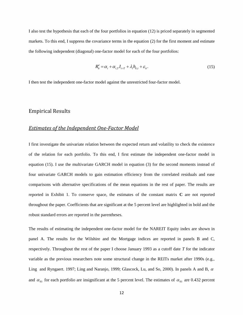
Exhibit 5 (panels A-D) reports the results of estimating equations (15)-(16). Panel A presents the results
for the one-factor model in which only the MKT volatility is the explanatory variable for the REIT return.
In panel B the REIT volatility is the second factor. Panel C includes the volatility of MKT, SMB and
HML and panel D includes the volatility of REIT as the fourth factor. Finally, panel E reports the results
of estimating a four-factor model with unrestricted risk prices (see notes to Exhibit 5).
Although alphas are not significant for each portfolio including REIT in panel A, the coefficient is -
0.067 with a standard error of 1.471, implying an insignificant relation between the expected REIT return
and the volatility of MKT. In panel B, the coefficient on the MKT volatility is -1.039 with a standard
error of 1.186 but the coefficient on the REIT volatility is 2.089 with a standard error of 0.979. Similar to

20
the covariance between MKT and REIT returns, the stock market volatility does not explain the positive
relation between the expected return and volatility of REIT.
In panels C and D, none of the estimated associated with the first three factors are two standard errors
away from zero. However, the coefficient associated with the REIT volatility is 2.139 with a standard
error of 0.481. Unlike the covariance-based model, the alphas in the three- and four-factor models in the
post-1993 period are significant. Strikingly, even for the unrestricted model in panel E, the coefficient
associated with the REIT volatility is significant but the coefficient associated with the volatility of each
other factor is not significant. The variance ratios associated with the REIT volatility in the four-factor
models exceed unity. Thus unlike the covariance-based model, the volatility of the Fama-French factors
do not explain the positive relation between the expected return and volatility of the REIT index.
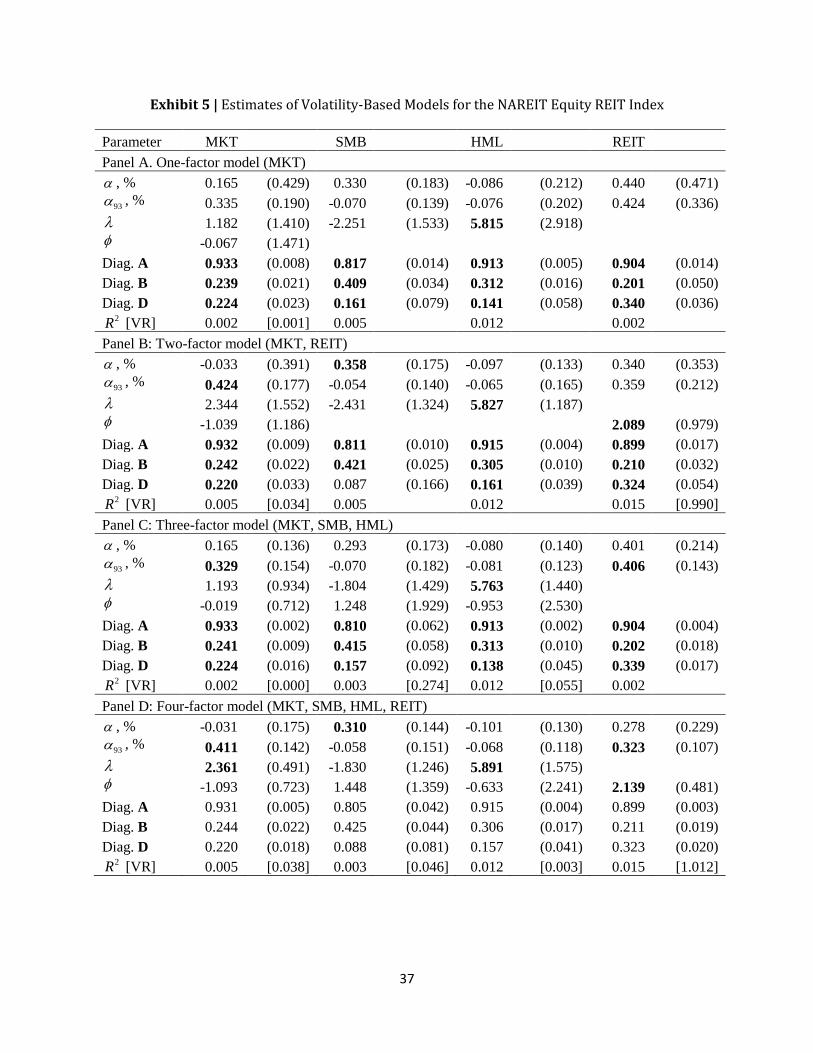
Exhibit 6 presents the results of estimating the volatility-based model using the Wilshire index. The
results are largely similar to those presented in Exhibit 5 for the NAREIT Equity REIT index. The
coefficient on MKT or other factor volatility in the one- to four-factor models is not significant but the
coefficient on the REIT volatility is more than two standard errors away from zero in either the two- or
four-factor model. Exhibit 7 reports the results of specification tests of the volatility-based models. The
maximized value of the log likelihood function for each volatility-based model here is sometimes higher
than that in the covariance-based model with the same number of factors in Exhibit 4 because the
volatility-based models involve more parameters. The maximized value of the log likelihood function for
the three-factor model without the REIT factor is lower than the value of the function for the two-factor
model including the REIT factor, suggesting poor performance of the three-factor volatility-based model.
The estimated alphas in the two or four models are jointly significant, with either the NAREIT index or
the Wilshire index. The results differ from those in the covariance-based models where alphas in only
one- and two-factor models are significant (see Exhibit 4). Likelihood ratio tests here in panel B do not
reject the one-factor model in favor of the three-factor model but reject the three-factor model in favor of

21
the four-factor model with either REIT index. Lastly, there is some significant evidence against the
hypothesis that risk prices are zero but the evidence is limited only to the NAREIT index. Overall, the
results here offer evidence that the covariances of REIT with risk factors are more useful than the
volatility of the factors in explaining the time variation of the expected REIT return.
Time-Series Properties of Expected Returns and Volatility of REITs
Given the similarity of the results obtained from the two REIT indices, in this section I examine the time-
series properties of the expected return and volatility of REITs implied by the covariance-based three-
factor model for the NAREIT Equity REIT index. Coefficients estimates in Exhibit 2, panel C are
assumed to be given.
Graphical Illustrations
To compare the expected excess return on the REIT index with its volatility, the expected REIT return is
plotted along with its volatility (standard deviation) in Exhibit 8. Large variations of the expected excess
return and volatility are observed in the four decades of our sample period, especially during the 2007-
2009 financial crisis. The sharp increase of the conditional REIT volatility during the crisis is consistent
with the recent evidence provided by Sun, Titman and Twite (2015). During the peak of the latest
financial crisis, the expected return increases to approximately eight times and the volatility increases to
approximately four times of their pre-crisis levels.
Exhibit 9 illustrates the decomposition of the REIT variance into the systematic and idiosyncratic
components given by equation (10). Similar to the expected REIT return, the total variance declines
slightly from the first decade to the second and third decades (from early 1980s’to late 1990s) then
increases sharply during the financial crisis. In periods of high volatility (the first and last decades), the
contribution of the systematic variance tends to much higher than that of the idiosyncratic variance. For

22
the full sample period, the systematic variance contributes an average of 53.3 percent of total variance.
Around the peak of the recent financial crisis (from Nov. 2008 to July 2009), the systematic variance
accounts for more than 80 percent of the total variance.
Exhibit 10 plots betas and factor risk premiums. The decreasing pattern of the stock market beta in the
first three decades, as reported by Khoo, Hartzell and Hoesli (1993), and Chiang, Lee and Wisen (2005),
is completely reversed in the last decade. Similar to the stock market beta and other betas, the stock
market premium and the value premium tend to be higher in the most recent decade. Thus the betas and
risk premiums contribute to the increases in the expected REIT return beginning in the early 2000s,
especially during the recent financial crisis. Exhibit 11 plots the volatility of each factor and the
correlation between each pair of the factors. The level of the stock market volatility during the financial
crisis is similar to that during the mid-1970s and late-1980s. Consistent with the results in Peterson and
Hsieh (1996), the correlation 13 between MKT and HML tends to be negative (close to -0.50) and lower
than other correlations most of times. However, the correlation13 surges quickly to positive levels during
the mid- to late-1970s and surges to unusually high and positive levels (0.50) during the 2007-2009
financial crisis. A comparison of Exhibits 10-11 reveals that the stock market premium and the correlation
13 increase more sharply during the recent financial crisis than the volatility of the stock market or other
factors.
Cross-Correlations
Exhibit 12 presents cross-correlations between pairs of the moments implied by the three-factor model
with the NAREIT equity REIT index. In fact, the expected REIT return, 4( )eE R , is highly correlated with
its own volatility, 44h , with a correlation of 0.873. However, as the results in Exhibit 2 show, the three
risk factors subsume the role of the REIT volatility in explaining the expected REIT return. Consistent
with the result, the expected REIT return, 4( )eE R , is very highly correlated with the stock market

23
premium 1 (correlation = 0.933), the HML beta
3 (correlation = 0.650), and the market beta 1
(correlation = 0.584).
As discussed earlier, the risk premium on each factor is proportional to the conditional factor volatility if
the factors are conditionally uncorrelated. Since the average correlations of returns on the stock market
portfolio and two factor-mimicking portfolios are relatively small (absolute values of average correlations
are less than 0.31), the risk premium on each factor should be more related to its own volatility than the
volatility of other factors. The correlation of the stock market premium 1 with its volatility
11h is 0.593
and the correlation of the HML premium 3 with its volatility
33h is 0.848. The SMB premium 2 is
negatively correlated to its volatility 22h , as a result of the negative risk price associated with this factor.
In addition to the factor volatility, equation (8) implies that the risk premium on each factor can be related
to its correlations with other factors. Exhibit 12 reports that the stock market premium is more highly
correlated with the MKT-HML correlation13 (correlation = 0.766) than the stock market volatility
(correlation = 0.610). Similarly, the correlation of the expected REIT return with the correlation 13 is
0.721 while the correlation with the stock market volatility 11h is only 0.528. To a lesser extent, the HML
premium is positively correlated with 13 , given the correlation of 0.270.
Next, I examine the implied volatility of the REIT return, 44h . Consistent with the high correlation
between the expected return and volatility of REIT, the correlations between the REIT volatility and other
moments in Exhibit 12 tend to be quite similar to the correlations between the expected REIT returns and
the moments. For example, the REIT volatility is more highly correlated with the stock market premium
than the HML premium, more highly correlated with the MKT-HML correlation 13 than the stock
market volatility, and correlated to a large extent with the MKT and HML betas.

24
Regression Results
As discussed in the introduction section, previous studies attribute the time variation in expected returns
on REITs to time-varying risk premiums and volatility (Li and Wang 1995; Devaney, 2001), or time-
varying betas associated with the stock market portfolio or other common factors (Khoo, Hartzell and
Hoesli, 1993; Liang, McIntosh and Webb, 1995; Chiang, Lee and Wisen, 2005). To discern the relative
importance of sources of the time-varying expected REIT return, I use linear approximations of equation
(9) to perform linear regressions, in which the independent variables include REIT betas, factor variances
and correlations between pairs of the factors. To understand why the REIT volatility loses its explanatory
power for the expected REIT return in the three-factor model studied earlier, I also perform similar
regressions of the variance of REIT return, using linear approximation of equation (10). The coefficient
estimates in the regressions are presented in Exhibit 13 with standard errors in parentheses. In panel A,
the dependent variable is the expected REIT return while in panel B the dependent variable is the variance
of the REIT index. All standard errors are adjusted for heteroskedasticity and residual autocorrelations up
to 24 (two years) lags. Any further increases in the lag length do not affect the results in any significant
way. As the independent variables are estimated from our sample and subject to the errors-in-variables
problem, the standard errors here are likely to be underestimated. As a result, coefficients that that
significant at the 1 percent rather than the usual 5 percent level are highlighted in bold. All coefficients
and standard errors are multiplied by 100 except for those associated with variances .iih
Panel A or B reports results of four regressions. The first regression reported in column (1) includes the
1993 indicator plus all of nine independent variables (betas, variances and correlations between pairs of
factors). The second to fourth regressions reported in columns (2) to (4) include three independent
variables (betas, variances or correlations). This time indicator is significant for the expected return but
not for the volatility (not reported). I first discuss the results in column (1). The results in panel A indicate
that the MKT and HML betas, the variances of MKT and SMB and the correlation between MKT and

25
HML are significant at the 1 percent level for explaining the expected REIT return. All coefficients on
these variables are positive except that on the SMB variance 22.h The coefficient associated with the
stock market beta is 1.377, which far exceeds the coefficient of 0.468 associated with the HML beta,
suggesting that the expected REIT return is more sensitive to the market beta than other betas. The results
in panel B show that the stock market and SMB betas, the variance of MKT and the correlation between
MKT and HML are significant at the 1 percent level for explaining the REIT volatility. Comparing with
the results in panel A, I find that the stock market beta and variance, along with the correlation between
MKT and HML, are significant in explaining both the expected REIT return and volatility. The adjusted
2R s of the regressions are 0.824 in panel A for the expected return and 0.797 for the volatility in panel B.
The similar and high 2R s offer further evidence that the systematic risks associated with the factor-
mimicking portfolios explain most of the time series movements of the expected REIT return and
volatility.
Next, I examine results in columns (2)-(4). The coefficients on the betas in column (2) of panels A and B
tend to be greater than those in column (1) but the statistical significance of the betas are largely
unchanged when the betas are the only independent variables. The results in column (3) indicate that the
variances of the factors are not significant at the 1 percent level for explaining either the mean or the
variance of the REIT returns when other independent variables are excluded from the regression. The loss
of the statistical significance is an example of the missing-variables problem. The results in column (4)
show that the correlation 13 between MKT and HML remains significant in explaining the expected
REIT return and volatility when the correlations between factors are the only independent variables.
Finally, the adjusted 2R s in columns (2)-(4) are respectively 0.613, 0.467 and 0.564 in panel A and.635,
0.379 and 0.397 in panel B. The sizes of the adjusted 2R s along with the significance of the coefficients
suggest that the betas and factor correlations are more important than the market and factor volatility for
explaining the expected REIT return and volatility.

26
Conclusions
This article uses conditional covariance-based three and four models to study the time variation of
expected returns on REITs. In the four-factor model, expected returns on REITs are related to their own
volatility and their covariances with the Fama-French factors. I apply the model to the NAREIT equity
REIT index from January 1972 to July 2013 and the Wilshire REIT index from January 1978 to July
2013. Estimation results obtained from both data sets suggest that the covariances of REIT returns with
the Fama-French factors subsume the role of the REIT volatility in explaining the expected REIT returns,
especially around the peak of the recent financial crisis (late-2008 to mid-2009). The finding differs from
other explanations of the REIT returns around the financial crisis based on firm-specific characteristics
(e.g., Sun, Titman and Twite. 2015). The evidence suggests that expected REIT returns are not
compensation for their own volatility but compensation for the risks associated with the stock market
premium and the value premium. The result here is consistent with the notion that the market for REITs is
integrated with the general stock market.
Capital market integration not only requires assets in different markets to be priced by common factors
but also requires the prices of risks associated with the factors to be the same across the markets. I find
that the risk prices associated with the REIT portfolio are not significantly different from those associated
with the three factor portfolios at the 5 percent level. I also find that an independent one-factor model for
each factor or the REIT portfolio, in which the expected return on each portfolio is related only to its own
volatility, is rejected in favor of a full four-factor model with covariance terms and unrestricted risk
prices. The result further supports the hypothesis that the market for REITs is integrated with that for the
factor portfolios.
Extending the evidence reported in the real estate literature (DeLisle, Price and Sirmans, 2013), this paper
documents that expected returns on REITs are insignificantly related to not only the volatility of the stock
market but also the volatility of the Fama-French factors. Expected returns on REITs in the covariances-
based three-factor model, therefore, are more useful than those in the volatility-based models in practical

27
applications, including constructions of efficient portfolios for investors and the performance evaluation
of fund managers. Since expected REIT returns tend to vary with systematic risks associated with the
common factors, especially during the financial crisis, it is essential to obtain precise and latest estimates
of time-varying covariance risks of REITs associated with the factors. As shown in the paper, the
estimated time-varying covariance risks can be transformed into estimates of time-varying betas
associated with the factors and time-varying factor risk premiums. The asymmetric multivariate GARCH-
in-means model serves as a useful tool for obtaining dynamic estimates of expected returns and risks of
REITs.
1 Fama and French (1996) conjecture that the value premium is linked to human capital. Jagannathan and Wang
(1996) find that the variability of labor income explains part of the value premium. See also Zhang (2005), Petkova
(2006), and Lettau and Wachter (2007) for more explanations of the value premium.
2Cotter and Stevenson (2006) use the multivariate VAR-GARCH model to document the return and volatility
linkages between REIT sub-sectors and inferences of other U.S. equity series. Yang, Zhou and Leung (2012) apply a
multivariate asymmetric generalized dynamic conditional correlation GARCH model to REITs and other assets and
find asymmetric volatility of REITs and asymmetric correlation of REITs with stock returns.
3 Other researchers (Myer, Chaudhry and Webb, 1996; Glascock, Lu, and So, 2000; Yunus, 2012) apply time series
techniques to examine the dynamic interaction of the real estate market with other markets. These techniques are
used to obtain insights into the long-run (co)integration of different markets unlike asset pricing models which are
often used in tests of various restrictions implied by the models.
4Since temporal aggregation would dilute certain characteristics of time series such as volatility clustering, the
multivariate GARCH model employed in the paper is best suited for data of higher frequency (daily or weekly)
rather than monthly. In a later section I will some perform sensitivity analysis with daily data.
5 The independent one-factor model is applied to daily data of MKT, SMB, HML or the NAREIT Equity REIT
index (or the NAREIT Mortgage REIT index) for the period from Feb. 24, 2006 to Aug. 29, 2014. For the short
sample period, the relation between the expected return on either REIT index and its volatility is not significant at
the 5 percent level when either the diagonal or full asymmetric GARCH model in equation (3) is used.

28
References
Campbell, J. Y. Stock Returns and the Term Structure. Journal of Financial Economics, 1987, 18, 373–
399.
Chiang, K., M. Lee and C. Wisen. Another Look at the Asymmetric REIT-Beta Puzzle. Journal of Real
Estate Research, 2004, 26, 25–42.
Chiang, K., M. Lee and C. Wisen. On the Time-Series Properties of Real Estate Investment Trust Betas.
Real Estate Economics, 2005, 33, 381-396.
Chou, Y. H., Y. C. Chen. Is the Response of REIT Returns to Monetary Policy Asymmetric? Journal of
Real Estate Research, 2014, 36, 109-135.
Cotter, J. and S. Stevenson. Multivariate Modeling of Daily REIT Volatility. Journal of Real Estate
Finance and Economics, 2006, 32, 305–25.
DeLisle, R. J., S. M. Price and C. F. Sirmans. Pricing of Volatility Risk in REITs. Journal of Real Estate
Research, 2013, 35, 223-248.
De Santis, G. and B. Gerard. International Asset Pricing and Portfolio Diversification with Time-Varying
Risk. Journal of Finance, 1997, 52, 1881–1912.
Devaney, M. Time-Varying Risk Premia for Real Estate Investment Trusts: A GARCH-M Model.
Quarterly Review of Economics and Finance, 2001, 41, 335–346.
Engle, R. F., and K. F. Kroner. Multivariate Simultaneous Generalized ARCH. Econometric Theory,
1995, 11, 122–150.
Flannery, M. J., A. S. Hameed, and R. H. Harjes. Asset Pricing, Time-varying Risk Premia and Interest
Rate Risk, Journal of Banking & Finance, 1997, 21, 315-335.
Fama, E. F. and K. R. French. Common Risk Factors in the Returns on Stocks and Bonds, Journal of
Financial Economics, 1993, 33, 3–56.
Fama, E. F. and K. R. French. Multifactor Explanations of Asset Pricing Anomalies, Journal of Finance,
1996, 51, 55-84.
Glascock, J., C. Lu, and R. So. Further Evidence on the Integration of REIT, Bond and Stock Returns.
Journal of Real Estate Finance and Economics, 2000. 20, 177-194.
Glosten, L. R., R. Jagannathan and D. E. Runkle. On the Relation between the Expected Value and the
Volatility of the Nominal Excess Return on Stocks. Journal of Finance, 1993, 48, 1779–1801.
Guo, H., R. Savickas, Z. Wang and J. Yang. Is the Value Premium a Proxy for Time-Varying Investment
Opportunities? Some Time-Series Evidence, Journal of Financial and Quantitative Analysis, 2009, 44,
133-154

29
Hardouvelis, G., A. D. Malliaropulos and R. Priestley. EMU and European Stock Market Integration.
Journal of Business, 2006, 79, 365-392.
Jaganathan, R. and Z. Wang. The Conditional CAPM and the Cross-Section of Expected Returns. The
Journal of Finance, 1996, 51, 3-53.
Khoo, T., D. Hartzell and M. Hoesli. An Investigation of the Change in Real Estate Investment Trust
Betas. Journal of American Real Estate and Urban Economics Association, 1993, 21, 107–130.
Kroner, K. E. and V. K. Ng. Model Asymmetric Comovements of Asset Returns. Review of Financial
Studies, 1998, 11, 817–844.
Lettau, M. and J. A. Wachter. Why Is Long-Horizon Equity Less Risky? A Duration-Based Explanation
of the Value Premium. Journal of Finance, 2007, 62, 55–92.
Li, Y. and K. Wang. The Predictability of REIT Return and Market Segmentation. Journal of Real Estate
Research, 1995. 10, 471-482.
Liang, Y., W. McIntosh and J. R. Webb. Intertemporal Changes in the Riskiness of EREITs. Journal of
Real Estate Research, 1995, 10, 427–443.
Ling, D. and A. Naranjo. The Integration of Commercial Real Estate Markets and Stock Markets. Real
Estate Economics, 1999, 27, 483–515.
Ling, D., and M. Ryngaert. Valuation Uncertainty, Institutional Involvement, and the Underpricing of
IPOs: The Case of REITs. Journal of Financial Economics, 1997, 43:3, 433-456.
Liu, C., D. Hartzell, W. Greig and T. Grissom. The Integration of Real Estate Market and the Stock
Market: Some Preliminary Evidence. Journal of Real Estate Finance and Economics, 1990, 3, 261-282.
Myer, F.C.N., M.K. Chaudhry, and J.R. Webb. Stationarity and Co-Integration in Systems with Three
National Real Estate Indices. Journal of Real Estate Research, 1996, 13, 369-81.
Mei, J. and A. Lee. Is There a Real Estate Factor Premium? Journal of Real Estate Finance and
Economics, 1994. 9:2, 113-126.
Merton, R. C., An Intertemporal Capital Asset Pricing Model. Econometrica, 1973. 41, 867-888.
Petkova, R. Do the Fama-French Factors Proxy for Innovations in Predictive Variables? Journal of
Finance, 2006, 61, 581–612.
Peterson, J. and C. Hsieh. Do Common Risk Factors in the Returns on Stocks and Bonds Explain Returns
on REITs? Real Estate Economics, 1997. 25, 321–345.
Ross, S. A. Return, Risk and Arbitrage, in I. Friend and J. Bicksler, eds., Risk and Return in Finance,
Cambridge, Mass., Ballinger, 1976.
Sun, L, S., Titman and G. Twite. REIT and Commercial Real Estate Returns: A Post Mortem of the
Financial Crisis. Real Estate Economics. 2015, 43, 8-36.

30
Yang J., Y. Zhou and W. Leung. Asymmetric Correlation and Volatility Dynamics among Stock, Bond,
and Securitized Real Estate Markets. Journal of Real Estate Finance and Economics, 2012, 45, 491–521.
Yunus, N. Modeling Relationships among Securitized Property Markets, Stock Markets, and
Macroeconomic Variables, Journal of Real Estate Research, 2012, 34, 127-156.
Whitelaw, R. F. Time Variations and Covariations in the Expectation and Volatility of Stock Market
Returns. Journal of Finance, 1994, 49, 515–541.
Zhang, L. The Value Premium. Journal of Finance, 2005, 60, 67-102.
The author is grateful to four referees and especially the Editor, Ko Wang for constructive comments and
valuable suggestions on earlier drafts of the paper.
Yuming Li, California State University, Fullerton, CA 92834 or [email protected]

31
Exhibit 1 | Estimates of an Independent One-Factor Model for the REIT Indices
Parameter MKT
SMB
HML
REIT
Panel A. NAREIT equity REIT
, % -0.157 (0.399) 0.347 (0.233) -0.104 (0.185) 0.131 (0.245)
93 , % 0.432 (0.230) -0.055 (0.168) -0.061 (0.170) 0.395 (0.212)
2.947 (1.203) -2.293 (1.779) 5.906 (1.932) 1.975 (0.863)
Diag. A 0.931 (0.009) 0.812 (0.009) 0.915 (0.006) 0.898 (0.019)
Diag. B 0.244 (0.017) 0.422 (0.030) 0.304 (0.017) 0.212 (0.022)
Diag. D 0.218 (0.023) 0.082 (0.147) 0.163 (0.044) 0.323 (0.040) 2R [VR] 0.007
0.005
0.012
0.016 [0.811]
Panel B. Wilshire equity REIT
, % 0.197 (0.127) 0.486 (0.274) -0.230 (0.157) -0.046 (0.119)
93 , % 0.316 (0.200) -0.008 (0.211) 0.079 (0.199) 0.519 (0.322)
1.557 (1.055) -4.867 (3.104) 5.607 (1.725) 1.712 (0.526)
Diag. A 0.944 (0.001) 0.806 (0.062) 0.898 (0.010) 0.923 (0.004)
Diag. B 0.237 (0.010) 0.400 (0.048) 0.337 (0.020) 0.223 (0.014)
Diag. D 0.170 (0.019) 0.102 (0.101) 0.113 (0.050) 0.274 (0.023) 2R [VR] 0.002
0.017
0.013
0.015 [0.749]
Panel C. NAREIT mortgage REIT
, % 0.190 (0.358) 0.355 (0.231) 0.023 (0.198) -0.382 (0.390)
93 , % 0.801 (0.267) -0.033 (0.176) -0.196 (0.143) 1.159 (0.296)
0.272 (1.481) -2.701 (1.838) 4.700 (2.060) 0.074 (1.365)
Diag. A 0.940 (0.011) 0.806 (0.035) 0.911 (0.005) 0.891 (0.015)
Diag. B 0.282 (0.076) 0.396 (0.032) 0.321 (0.024) 0.234 (0.046)
Diag. D 0.123 (0.112) 0.078 (0.086) 0.182 (0.043) 0.375 (0.044) 2R [VR] 0.007
0.005
0.010
0.010 [0.001]
Notes: The excess return for each of the four portfolios is given by equation (15):
, , ,e
it i i T t T i ii t itR I h where i is the ith intercept for the period before date T (1993:01) and
iT is the incremental intercept for the period afterwards. The conditional variance-covariance matrix tH
follows the asymmetric BEKK GARCH specification: 1 1 1 1 1' ,t t t t t tH C C A'H A B'ε ε 'B D'η η 'D
where A, B and D are diagonal matrices and C is a lower triangular matrix, and 1tη is a vector with ith
element given by , 1 , 1i t i t if
, 1 0i t and zero otherwise. The excess returns for each model include
excess market returns (MKT), returns on small stocks minus returns on big stocks (SMB), returns on high
book-market stocks minus returns on low book-market stocks (HML), and excess returns on the REIT
index. The2R is the percentage of the variance of realized excess returns explained by the variance of
expected excess returns. VR is the variance of a component of the expected excess return on the REIT
index associated with a factor divided by the variance of the expected excess return on the REIT index.
Coefficients that are significant at the 5 percent level are highlighted in bold and the robust standard
errors are reported in the parentheses.

32
Exhibit 2 | Estimates of Covariance-Based Models for the NAREIT Equity REIT Index
Parameter MKT
SMB
HML
REIT
Panel A. One-factor model (MKT)
, % -0.153 (0.128) 0.030 (0.103) 0.448 (0.094) 0.058 (0.137)
93 , % 0.402 (0.185) -0.021 (0.149) -0.126 (0.132) 0.462 (0.229)
2.976 (0.925)
Diag. A 0.926 (0.013) 0.832 (0.041) 0.907 (0.007) 0.896 (0.015)
Diag. B 0.251 (0.030) 0.400 (0.043) 0.314 (0.022) 0.208 (0.034)
Diag. D 0.232 (0.046) 0.159 (0.101) 0.178 (0.071) 0.345 (0.053) 2R [VR] 0.007 [0.735] 0.001 0.003 0.010
Panel B: Two-factor model (MKT, REIT)
, % -0.031 (0.116) -0.003 (0.094) 0.388 (0.087) -0.039 (0.118)
93 , % 0.345 (0.177) -0.032 (0.137) -0.130 (0.140) 0.378 (0.153)
1.411 (0.882)
1.749 (0.779)
Diag. A 0.928 (0.002) 0.831 (0.009) 0.908 (0.004) 0.895 (0.003)
Diag. B 0.251 (0.011) 0.401 (0.018) 0.316 (0.014) 0.211 (0.015)
Diag. D 0.226 (0.018) 0.157 (0.059) 0.170 (0.034) 0.335 (0.014) 2R [VR] 0.009 [0.067] 0.001
0.003
0.025 [0.475]
Panel C: Three-factor model (MKT, SMB, HML)
, % 0.120 (0.129) 0.312 (0.141) 0.034 (0.141) 0.175 (0.139)
93 , % 0.311 (0.162) -0.008 (0.138) -0.141 (0.176) 0.355 (0.230)
3.597 (0.841) -3.504 (1.490) 6.516 (2.124)
Diag. A 0.926 (0.006) 0.831 (0.036) 0.910 (0.008) 0.898 (0.010)
Diag. B 0.246 (0.022) 0.389 (0.042) 0.314 (0.026) 0.204 (0.028)
Diag. D 0.235 (0.024) 0.192 (0.053) 0.159 (0.045) 0.337 (0.016) 2R [VR] 0.012 [0.392] 0.032 [0.023] 0.018 [0.221] 0.027
Panel D: Four-factor model (MKT, SMB, HML, REIT)
, % 0.113 (0.181) 0.310 (0.169) 0.031 (0.155) 0.181 (0.229)
93 , % 0.314 (0.200) -0.007 (0.154) -0.141 (0.128) 0.360 (0.250)
3.733 (1.633) -3.440 (1.583) 6.649 (2.362) -0.149 (1.724)
Diag. A 0.925 (0.013) 0.831 (0.044) 0.910 (0.013) 0.898 (0.019)
Diag. B 0.246 (0.028) 0.389 (0.056) 0.313 (0.031) 0.203 (0.031)
Diag. D 0.235 (0.037) 0.192 (0.137) 0.160 (0.063) 0.338 (0.046) 2R [VR] 0.012 [0.439] 0.032 [0.023] 0.018 [0.239] 0.025 [0.003]

33
Exhibit 2 (Continued) Estimates of Covariance-Based Models for the NAREIT Equity REIT Index
Parameter MKT SMB HML REIT
Panel E: Four-factor model with unrestricted risk prices (MKT, SMB, HML, REIT)
, % -0.285 (0.455) -0.286 (0.312) 0.232 (-0.210) -0.580 (0.494)
93 , % 0.373 (0.280) -0.009 (0.195) 0.061 (0.202) 0.442 (0.306)
MKT 2.469 (2.562) 1.256 (4.719) -1.317 (5.993) 0.980 (2.830)
SMB 8.278 (4.659) -2.737 (3.369) 5.286 (6.265) 6.157 (6.236)
HML -0.791 (2.520) -6.048 (3.851) 6.366 (2.390) -2.583 (3.886)
REIT -1.976 (3.441) 15.358 (8.405) -4.916 (6.964) 2.647 (2.840)
Diag. A 0.929 (0.007) 0.830 (0.022) 0.915 (0.005) 0.900 (0.014)
Diag. B 0.247 (0.028) 0.410 (0.033) 0.302 (0.023) 0.198 (0.036)
Diag. D 0.230 (0.037) 0.095 (0.087) 0.173 (0.055) 0.332 (0.039) 2R [VR] 0.009 [0.143] 0.039 [0.393] 0.030 [0.155] 0.022 [1.149]
Notes: For panels A-D, the excess return for each of the four portfolios is given by equation (2):
, ,1
Ke
it i i T t T j ij t itjR I h
with restricted risk prices j . For panel E, the excess return is given
by equation (14): 4
, ,1
e
it i i T t T ij ij t itjR I h
with unrestricted risk prices ij . The conditional
variance-covariance matrix tH in each panel follows the asymmetric BEKK GARCH specification:
1 1 1 1 1' .t t t t t tH C C A'H A B'ε ε 'B D'η η 'D Coefficients that are significant at the 5 percent level
are highlighted in bold and the robust standard errors are reported in the parentheses.

34
Exhibit 3 | Estimates of Covariance-Based Models for the Wilshire REIT Index
Parameter MKT
SMB
HML
REIT
Panel A. One-factor model (MKT)
, % 0.395 (0.137) -0.031 (0.138) -0.003 (0.089) 0.113 (0.156)
93 , % 0.187 (0.211) -0.017 (0.178) 0.144 (0.117) 0.552 (0.171)
0.633 (0.276)
Diag. A 0.944 (0.006) 0.862 (0.027) 0.885 (0.022) 0.925 (0.009)
Diag. B 0.237 (0.031) 0.355 (0.058) 0.361 (0.046) 0.215 (0.048)
Diag. D 0.166 (0.071) 0.145 (0.084) 0.115 (0.119) 0.291 (0.069) 2R [VR] 0.001 [0.046] 0.000
0.001
0.003
Panel B: Two-factor model (MKT, REIT)
, % 0.242 (0.132) -0.013 (0.099) 0.168 (0.099) -0.153 (0.132)
93 , % 0.213 (0.179) -0.031 (0.130) 0.060 (0.137) 0.437 (0.159)
0.096 (1.024) 2.207 (0.798)
Diag. A 0.944 (0.002) 0.866 (0.007) 0.883 (0.007) 0.924 (0.003)
Diag. B 0.239 (0.010) 0.354 (0.016) 0.364 (0.017) 0.226 (0.013)
Diag. D 0.154 (0.021) 0.148 (0.070) 0.090 (0.072) 0.272 (0.016) 2R [VR] 0.005 [0.000] 0.001
0.003 0.024 [0.834]
Panel C: Three-factor model (MKT, SMB, HML)
, % 0.337 (0.331) -0.025 (0.223) 0.034 (0.249) 0.100 (0.321)
93 , % 0.225 (0.354) -0.031 (0.190) 0.072 (0.209) 0.555 (0.370)
0.198 (0.796) -1.498 (0.853) 2.872 (1.285)
Diag. A 0.942 (0.008) 0.804 (0.042) 0.895 (0.005) 0.921 (0.017)
Diag. B 0.239 (0.023) 0.404 (0.043) 0.347 (0.016) 0.225 (0.024)
Diag. D 0.178 (0.024) 0.078 (0.091) 0.093 (0.065) 0.288 (0.028) 2R [VR] 0.002 [0.003] 0.003 [0.174] 0.003 [0.352] 0.004
Panel D: Four-factor model (MKT, SMB, HML, REIT)
, % 0.331 (0.160) -0.044 (0.145) 0.002 (0.159) 0.089 (0.150)
93 , % 0.240 (0.235) -0.001 (0.153) 0.101 (0.154) 0.582 (0.242)
0.526 (0.410) -1.553 (0.868) 2.869 (1.259) -0.199 (0.235)
Diag. A 0.942 (0.008) 0.804 (0.062) 0.896 (0.017) 0.921 (0.019)
Diag. B 0.239 (0.022) 0.404 (0.056) 0.345 (0.035) 0.225 (0.036)
Diag. D 0.179 (0.043) 0.074 (0.081) 0.101 (0.079) 0.288 (0.046) 2R [VR] 0.002 [0.023] 0.003 [0.183] 0.004 [0.340] 0.004 [0.037]

35
Exhibit 3 (Continued) Estimates of Covariance-Based Models for the Wilshire REIT Index
Parameter MKT SMB HML REIT
Panel E: Four-factor model with unrestricted risk prices (MKT,SMB,HML,REIT)
, % 0.088 (0.999) -0.060 (0.303) -0.089 (0.188) -0.283 (3.351)
93 , % 0.385 (1.842) 0.041 (0.796) -0.007 (0.994) 0.439 (0.533)
MKT 5.470 (4.297)) -3.461 (9.335) -4.237 (20.336) -0.580 (1.900)
SMB 4.196 (0.959) -10.174 (20.932) 0.380 (13.008) -0.056 (0.321)
HML -3.689 (6.617) 7.644 (15.320) 7.766 (12.203) -0.256 (0.400)
REIT 1.287 (8.953) 3.138 (1.633) -1.780 (12.706) 1.153 (2.006)
Diag. A 0.941 (0.040) 0.801 (0.133) 0.903 (0.012) 0.922 (0.080)
Diag. B 0.232 (0.101) 0.389 (0.064) 0.326 (0.103) 0.214 (0.051)
Diag. D 0.188 (0.089) 0.102 (0.223) 0.132 (0.056) 0.286 (0.245) 2R [VR] 0.011 [0.048] 0.062 [0.160] 0.073 [0.026] 0.011 [0.466]
Notes: For panels A-D, the excess return for each of the four portfolios is given by equation (2):
, ,1
Ke
it i i T t T j ij t itjR I h
with restricted risk prices j For panel E, the excess return is given
by equation (14): 4
, ,1
e
it i i T t T ij ij t itjR I h
with unrestricted risk prices ij . The conditional
variance-covariance matrix tH in each panel follows the asymmetric BEKK GARCH specification:
1 1 1 1 1' .t t t t t tH C C A'H A B'ε ε 'B D'η η 'D Coefficients that are significant at the 5 percent level
are highlighted in bold and the robust standard errors are reported in the parentheses

36
Exhibit 4 | Specification Tests of Covariance-Based Models
Panel A. Log likelihood and joint significance of alphas
NAREIT Equity REIT Wilshire REIT
Log p-value
Log p-value
Number of factors Likelihood 93
Likelihood 93
Zero factor 4090.1 0.002 0.048
3500.5 0.031 0.574
One: MKT 4091.7 0.000 0.031
3500.8 0.031 0.004
Two: MKT,REIT 4092.2 0.000 0.000
3502.1 0.687 0.456
Three: MKT,SMB,HML 4096.8 0.260 0.125
3502.1 0.687 0.456
Four: MKT,SMB,HML,REIT
Restricted risk prices 4096.8 0.452 0.256
3502.3 0.228 0.073
Unrestricted risk prices 4108.1 0.427 0.391
3515.5 0.170 0.027
Panel B. Likelihood ratio (LR) tests
Hypothesis DF LR p-value
DF LR p-value
Zero vs. three-factor 3 13.3 0.004
3 3.1 0.370
One- vs. three-factor 2 10.3 0.006
2 2.5 0.283
Three- vs. four-factor 1 0.01 0.942
1 0.4 0.526
Four-factor: equal vs. diff. prices
MKT 4 3.7 0.446
4 2.9 0.579
SMB 4 7.2 0.125
4 7.8 0.098
HML 4 10.4 0.034
4 13.0 0.011
REIT 4 3.7 0.447
4 9.4 0.051
Four-factor
Restricted vs. unrestricted 12 22.5 0.032
12 26.4 0.010
Independent vs unrestricted 12 23.7 0.023 12 24.3 0.019
Notes: The independent model refers to the model in Exhibit 1. Other models are described in Exhibits 2-
3. Coefficients that are significant at the 5 percent level are highlighted in bold and the robust standard
errors are reported in the parentheses.
37
Exhibit 5 | Estimates of Volatility-Based Models for the NAREIT Equity REIT Index
Parameter MKT
SMB
HML
REIT
Panel A. One-factor model (MKT)
, % 0.165 (0.429) 0.330 (0.183) -0.086 (0.212) 0.440 (0.471)
93 , % 0.335 (0.190) -0.070 (0.139) -0.076 (0.202) 0.424 (0.336)
1.182 (1.410) -2.251 (1.533) 5.815 (2.918)
-0.067 (1.471)
Diag. A 0.933 (0.008) 0.817 (0.014) 0.913 (0.005) 0.904 (0.014)
Diag. B 0.239 (0.021) 0.409 (0.034) 0.312 (0.016) 0.201 (0.050)
Diag. D 0.224 (0.023) 0.161 (0.079) 0.141 (0.058) 0.340 (0.036) 2R [VR] 0.002 [0.001] 0.005
0.012
0.002
Panel B: Two-factor model (MKT, REIT)
, % -0.033 (0.391) 0.358 (0.175) -0.097 (0.133) 0.340 (0.353)
93 , % 0.424 (0.177) -0.054 (0.140) -0.065 (0.165) 0.359 (0.212)
2.344 (1.552) -2.431 (1.324) 5.827 (1.187)
-1.039 (1.186) 2.089 (0.979)
Diag. A 0.932 (0.009) 0.811 (0.010) 0.915 (0.004) 0.899 (0.017)
Diag. B 0.242 (0.022) 0.421 (0.025) 0.305 (0.010) 0.210 (0.032)
Diag. D 0.220 (0.033) 0.087 (0.166) 0.161 (0.039) 0.324 (0.054) 2R [VR] 0.005 [0.034] 0.005
0.012
0.015 [0.990]
Panel C: Three-factor model (MKT, SMB, HML)
, % 0.165 (0.136) 0.293 (0.173) -0.080 (0.140) 0.401 (0.214)
93 , % 0.329 (0.154) -0.070 (0.182) -0.081 (0.123) 0.406 (0.143)
1.193 (0.934) -1.804 (1.429) 5.763 (1.440)
-0.019 (0.712) 1.248 (1.929) -0.953 (2.530)
Diag. A 0.933 (0.002) 0.810 (0.062) 0.913 (0.002) 0.904 (0.004)
Diag. B 0.241 (0.009) 0.415 (0.058) 0.313 (0.010) 0.202 (0.018)
Diag. D 0.224 (0.016) 0.157 (0.092) 0.138 (0.045) 0.339 (0.017) 2R [VR] 0.002 [0.000] 0.003 [0.274] 0.012 [0.055] 0.002
Panel D: Four-factor model (MKT, SMB, HML, REIT)
, % -0.031 (0.175) 0.310 (0.144) -0.101 (0.130) 0.278 (0.229)
93 , % 0.411 (0.142) -0.058 (0.151) -0.068 (0.118) 0.323 (0.107)
2.361 (0.491) -1.830 (1.246) 5.891 (1.575)
-1.093 (0.723) 1.448 (1.359) -0.633 (2.241) 2.139 (0.481)
Diag. A 0.931 (0.005) 0.805 (0.042) 0.915 (0.004) 0.899 (0.003)
Diag. B 0.244 (0.022) 0.425 (0.044) 0.306 (0.017) 0.211 (0.019)
Diag. D 0.220 (0.018) 0.088 (0.081) 0.157 (0.041) 0.323 (0.020) 2R [VR] 0.005 [0.038] 0.003 [0.046] 0.012 [0.003] 0.015 [1.012]

38
Exhibit 5 (Continued) Estimates of Volatility-Based Models for the NAREIT Equity REIT Index
Parameter MKT SMB HML REIT
Panel E: Four-factor model with unrestricted risk prices (MKT, SMB, HML, REIT)
, % -0.284 (0.388) -0.286 (0.353) -0.210 (0.192) -0.580 (0.560)
93 , % 0.372 (0.266) -0.009 (0.247) 0.061 (0.170) 0.442 (0.317)
MKT 2.472 (1.871) 1.256 (5.206) -1.309 (4.786) 0.974 (1.940)
SMB 8.281 (3.550) -2.729 (2.712) 5.304 (6.311) 6.153 (6.408)
HML -0.779 (3.519) -6.029 (4.522) 6.382 (2.723) -2.601 (3.804)
-1.975 (2.921) 15.368 (11.987) -4.904 (5.155) 2.641 (1.118)
Diag. A 0.929 (0.010) 0.830 (0.018) 0.915 (0.014) 0.900 (0.020)
Diag. B 0.247 (0.031) 0.410 (0.036) 0.302 (0.030) 0.198 (0.035)
Diag. D 0.230 (0.038) 0.095 (0.126) 0.173 (0.051) 0.332 (0.044) 2R [VR] 0.009 [0.143] 0.039 (0.394) 0.030 [0.154] 0.021 [1.146]
Notes: For panels A-D, the factor risk premiums on MKT, SMB and HML are given by independent one-
factor models in equation (15): , ,
e
it i i T t T i ii t itR I h (i =1,2,3) and the excess REIT return is
given by equation (16): 4 4 4 , 41.
Ke
t T t T j jj t tjR I h
For panel E, the excess return is given by
equation (14): 4
, ,1
e
it i i T t T ij jj t itjR I h
with unrestricted risk prices ij . The conditional
variance-covariance matrix tH in each panel follows the asymmetric BEKK GARCH specification:
1 1 1 1 1' .t t t t t tH C C A'H A B'ε ε 'B D'η η 'D Coefficients that are significant at the 5 percent level
are highlighted in bold and the robust standard errors are reported in the parentheses.

39
Exhibit 6 | Estimates of Volatility-Based Models for the Wilshire Equity REIT Index
Parameter MKT
SMB
HML
REIT
Panel A. One-factor model (MKT)
, % 0.529 (0.337) 0.446 (0.294) -0.204 (0.195) 0.265 (0.215)
93 , % 0.248 (0.283) 0.007 (0.208) 0.051 (0.170) 0.573 (0.215)
-0.385 (0.974) -4.720 (2.678) 5.548 (2.002)
-0.224 (1.058)
Diag. A 0.944 (0.009) 0.810 (0.055) 0.896 (0.006) 0.925 (0.018)
Diag. B 0.233 (0.020) 0.394 (0.063) 0.342 (0.018) 0.214 (0.028)
Diag. D 0.179 (0.033) 0.126 (0.099) 0.095 (0.073) 0.290 (0.034) 2R [VR] 0.001 [0.006] 0.016
0.013
0.003
Panel B: Two-factor model (MKT, REIT)
, % 0.331 (0.430) 0.499 (0.190) -0.223 (0.182) 0.206 (0.429)
93 , % 0.310 (0.275) -0.005 (0.117) 0.072 (0.150) 0.482 (0.249)
0.883 (1.562) -5.027 (2.151) 5.570 (2.198)
-1.276 (1.746) 1.832 (0.521)
Diag. A 0.945 (0.009) 0.805 (0.011) 0.898 (0.008) 0.924 (0.018)
Diag. B 0.234 (0.022) 0.400 (0.030) 0.338 (0.025) 0.221 (0.033)
Diag. D 0.171 (0.035) 0.102 (0.091) 0.110 (0.069) 0.274 (0.034) 2R [VR] 0.001 [0.036] 0.018
0.013
0.014 [0.919]
Panel C: Three-factor model (MKT, SMB, HML)
, % 0.532 (0.293) 0.395 (0.274) -0.200 (0.203) 0.218 (0.337)
93 , % 0.239 (0.163) 0.000 (0.180) 0.044 (0.148) 0.529 (0.236)
-0.391 (1.481) -4.011 (2.628) 5.549 (2.060)
-0.314 (1.227) 1.935 (2.712) -0.953 (2.487)
Diag. A 0.945 (0.009) 0.805 (0.060) 0.896 (0.005) 0.926 (0.019)
Diag. B 0.234 (0.015) 0.397 (0.052) 0.342 (0.018) 0.213 (0.024)
Diag. D 0.178 (0.029) 0.126 (0.094) 0.091 (0.063) 0.287 (0.031) 2R [VR] 0.001 [0.010] 0.012 [0.280] 0.013 [0.034] 0.003
Panel D: Four-factor model (MKT, SMB, HML, REIT)
, % 0.328 (0.132) 0.433 (0.259) -0.225 (0.223) 0.127 (0.203)
93 , % 0.300 (0.166) -0.016 (0.176) 0.065 (0.153) 0.417 (0.240)
0.909 (1.077) -4.130 (2.495) 5.665 (2.217)
-1.473 (1.110) 2.276 (2.835) -0.815 (2.470) 1.920 (0.581)
Diag. A 0.945 (0.009) 0.800 (0.058) 0.898 (0.005) 0.925 (0.019)
Diag. B 0.235 (0.016) 0.402 (0.051) 0.338 (0.016) 0.220 (0.023)
Diag. D 0.170 (0.026) 0.103 (0.097) 0.104 (0.065) 0.270 (0.031) 2R [VR] 0.001 [0.046] 0.012 [0.083] 0.013 [0.006] 0.015 [0.953]
40
Exhibit 6 (Continued) Estimates of Volatility-Based Models for the Wilshire Equity REIT Index
Parameter MKT SMB HML REIT
Panel E: Four-Factor model with unrestricted risk prices (MKT, SMB, HML, REIT)
, % 0.303 (0.279) -0.170 (0.183) -0.349 (0.208) -1.182 (0.286)
93 , % 0.026 (0.222) -0.032 (0.133) 0.278 (0.196) 0.627 (0.238)
MKT 3.386 (0.603) 8.980 (5.340) 7.042 (3.835) -2.122 (0.991)
HML -0.962 (4.338) -7.966 (3.614) 4.695 (2.938) -3.486 (4.322)
-1.508 (1.103) 21.808 (3.757) -10.939 (2.999) 2.708 (0.318)
Diag. A 0.944 (0.004) 0.839 (0.043) 0.895 (0.010) 0.935 (0.004)
Diag. B 0.232 (0.021) 0.378 (0.045) 0.336 (0.024) 0.185 (0.022)
Diag. D 0.176 (0.026) 0.127 (0.079) 0.153 (0.046) 0.271 (0.017) 2R [VR] 0.007 [0.051] 0.048 [0.658] 0.038 [0.603] 0.026 [0.984]
Notes: For panels A-D, the factor risk premiums on MKT, SMB and HML are given by the independent
one-factor model in equation (15): , ,
e
it i i T t T i ii t itR I h (i =1,2,3) and the excess REIT return is
given by equation (16): 4 4 4 , 41.
Ke
t T t T j jj t tjR I h
For panel E, the excess return is given by
equation (14): 4
, ,1
e
it i i T t T ij jj t itjR I h
with unrestricted risk prices ij . The conditional
variance-covariance matrix tH in each panel follows the asymmetric BEKK GARCH specification:
1 1 1 1 1' .t t t t t tH C C A'H A B'ε ε 'B D'η η 'D Coefficients that are significant at the 5 percent level
are highlighted in bold and the robust standard errors are reported in the parentheses.

41
Exhibit 7 | Specification Tests of Volatility-Based Models
Panel A. Log likelihood and joint significance of alphas
NAREIT EREIT Wilshire EREIT
Log p-value
Log p-value
Number of factors Likelihood 93
Likelihood 93
One: MKT 4093.9 0.417 0.031
3503.3 0.017 0.075
Two: MKT REIT 4096.4 0.004 0.055
3505.4 0.016 0.259
Three: MKT, SMB, HML 4094.2 0.000 0.009
3503.6 0.255 0.145
Four: MKT,SMB,HML, REIT 4096.7 0.000 0.000
3505.9 0.010 0.256
Four: unrestricted risk prices 4108.1 0.552 0.583 3517.3 0.000 0.090
Panel B. Likelihood ratio (LR) tests
Hypothesis DF LR p-value
DF LR p-value
Zero vs. three-factor 3 8.1 0.044
3 6.2 0.102
One vs. three factors 2 0.5 0.782
2 0.7 0.711
Three vs. four factors 1 5.1 0.023
1 4.5 0.034
Independent vs. unrestricted 12 23.3 0.025
12 20.6 0.057
Notes: The independent model refers to the model in Exhibit 1. Other models are described in Exhibits 5-
6.

42
Exhibit 12 | Correlations of Expected REIT Return, Volatility and Other Moments
Variance Risk Premium Beta Variance Correlation
REIT MKT SMB HML MKT SMB HML MKT SMB HML (M,S) (M,H) (S,H)
44h 1 2
3 1 2
3 11h 22h
33h 12 13
23
4( )eE R 0.873 0.933 0.129 0.395 0.584 0.326 0.650 0.528 0.007 0.294 0.088 0.721 0.209
44h 0.776 0.160 0.294 0.622 0.409 0.586 0.610 -0.001 0.225 0.210 0.622 0.210
1
0.074 0.347 0.475 0.286 0.589 0.593 0.057 0.253 0.009 0.766 0.246
2
-0.656 0.233 -0.001 -0.104 0.061 -0.787 -0.486 0.337 0.122 0.735
3
-0.018 0.189 0.344 0.346 0.600 0.848 -0.201 0.270 -0.412
1
-0.065 0.489 0.235 -0.086 -0.067 0.240 0.480 0.244
3
0.186 0.279 -0.017 0.167 0.020 0.104 0.007
3
0.324 0.139 0.292 -0.101 0.448 0.004
11h
0.166 0.468 0.180 0.275 0.198
22h
0.528 -0.148 0.033 -0.641
33h
-0.220 0.070 -0.297
12
0.156 0.063
13
0.296
Notes: 4( )eE R is the expected excess return on the REIT index. The results are implied by the covariance-based three-factor model (see Exhibit 2,
panel C.)

43
Exhibit 13 | Regression on Factor Betas, Volatility and Correlations
(1) (2) (3) (4) Panel A. Dependent variable: expected REIT return
Constant -0.608 (0.240)
-1.906 (0.743)
-0.394 (0.376)
1.392 (0.374)
I(t>93) 0.281 (0.060)
0.295 (0.094)
0.690 (0.184)
0.377 (0.110)
1 1.377 (0.244)
2.210 (0.638)
2 0.781 (0.404)
1.318 (0.707)
3 0.468 (0.164)
1.210 (0.362)
11h 1.999 (0.321)
3.916 (1.712)
22h -1.986 (0.598)
-1.485 (1.432)
33h 1.829 (1.086)
0.956 (2.917)
12 -0.353 (0.154)
-0.027 (0.193)
13 1.708 (0.344)
2.472 (0.928)
23 -0.478 (0.225)
0.212 (0.183)
Adj. 2R 0.824
0.613
0.467
0.564
Panel B. Dependent variable: variance of REIT return
Constant -0.555 (0.196)
-0.872 (0.308)
-0.153 (0.167)
0.447 (0.142)
1 0.760 (0.177)
1.067 (0.280)
2 0.459 (0.132)
0.662 (0.236)
3 0.162 (0.078)
0.366 (0.143)
11h 0.981 (0.327)
1.690 (0.870)
22h -0.509 (0.228)
-0.332 (0.468)
33h 0.074 (0.285)
-0.129 (0.921)
12 0.004 (0.085)
0.215 (0.078)
13 0.440 (0.123)
0.826 (0.374)
23 -0.225 (0.125)
0.054 (0.060)
Adj. 2R 0.797
0.635
0.379
0.397
Notes: Coefficients estimates in Exhibit 2, panel C are given. All coefficients and standard errors are
multiplied by 100 except for those associated with .iih Coefficients that are significant at the 1 percent
level are highlighted in bold and robust standard errors are reported in parentheses.

44
Exhibit 8 | Expected Returns and Volatility of the NAREIT Equity REIT Index
.
0
2
4
6
8
10
12
14
16
18
20
-1
0
1
2
3
4
5
6
7
8
19
72
03
19
73
11
19
75
07
19
77
03
19
78
11
19
80
07
19
82
03
19
83
11
19
85
07
19
87
03
19
88
11
19
90
07
19
92
03
19
93
11
19
95
07
19
97
03
19
98
11
20
00
07
20
02
03
20
03
11
20
05
07
20
07
03
20
08
11
20
10
07
20
12
03
Std
. De
v.,
%
Exp
ect
ed
exc
ess
re
turn
, %
Expected Return Volatility

45
Exhibit 9 | Systematic and Idiosyncratic Variances of the NAREIT Equity REIT Index
0
50
100
150
200
250
300
19
72
03
19
73
09
19
75
03
19
76
09
19
78
03
19
79
09
19
81
03
19
82
09
19
84
03
19
85
09
19
87
03
19
88
09
19
90
03
19
91
09
19
93
03
19
94
09
19
96
03
19
97
09
19
99
03
20
00
09
20
02
03
20
03
09
20
05
03
20
06
09
20
08
03
20
09
09
20
11
03
20
12
09
Var
ian
cex1
0,0
00
Systematic Idiosyncratic

46
Exhibit 10 | Conditional Betas and Factor Risk Premiums
Panel A: Betas
Panel B: Factor risk premiums.
-0.5
0
0.5
1
1.5
19
72
03
19
74
03
19
76
03
19
78
03
19
80
03
19
82
03
19
84
03
19
86
03
19
88
03
19
90
03
19
92
03
19
94
03
19
96
03
19
98
03
20
00
03
20
02
03
20
04
03
20
06
03
20
08
03
20
10
03
20
12
03
Cco
rre
lati
on
an
d b
eta
Market SMB HML
-1
0
1
2
3
4
5
19
72
03
19
73
09
19
75
03
19
76
09
19
78
03
19
79
09
19
81
03
19
82
09
19
84
03
19
85
09
19
87
03
19
88
09
19
90
03
19
91
09
19
93
03
19
94
09
19
96
03
19
97
09
19
99
03
20
00
09
20
02
03
20
03
09
20
05
03
20
06
09
20
08
03
20
09
09
20
11
03
20
12
09
Exp
ect
ed
exc
ess
re
turn
, %
Market SMB HML

47
Exhibit 11 | Conditional Factor Volatility and Correlations
Panel A: Factor volatility
Panel B: Factor correlations
0
1
2
3
4
5
6
7
8
9
10
19
72
03
19
73
09
19
75
03
19
76
09
19
78
03
19
79
09
19
81
03
19
82
09
19
84
03
19
85
09
19
87
03
19
88
09
19
90
03
19
91
09
19
93
03
19
94
09
19
96
03
19
97
09
19
99
03
20
00
09
20
02
03
20
03
09
20
05
03
20
06
09
20
08
03
20
09
09
20
11
03
20
12
09
Std
. de
v., %
Market SMB HML
-1-0.8-0.6-0.4-0.2
00.20.40.60.8
1
19
72
03
19
74
03
19
76
03
19
78
03
19
80
03
19
82
03
19
84
03
19
86
03
19
88
03
19
90
03
19
92
03
19
94
03
19
96
03
19
98
03
20
00
03
20
02
03
20
04
03
20
06
03
20
08
03
20
10
03
20
12
03
Cco
rre
lati
on
(MKT,SMB) (MKT,HML) (SMB,HML)


![[Najib Razali] Islamic REITS - prres.net REITs.pdfDo Islamic REITs Behave Differently from Conventional REITs? – Empirical Evidence from Malaysian REITs Sing Tien Foo National University](https://img.pdfslide.us/doc/110x75/5abe8db57f8b9a7e418d14eb/najib-razali-islamic-reits-prres-reitspdfdo-islamic-reits-behave-differently.jpg)


![Time Variation in the Covariance between Stock Returns and …1673-1712]jofi_777.pdf · 2008-07-22 · Time Variation in the Covariance between Stock Returns and Consumption Growth](https://img.pdfslide.us/doc/110x75/5b9ef5c209d3f2083f8c696a/time-variation-in-the-covariance-between-stock-returns-and-1673-1712jofi777pdf.jpg)