Time-VariantGas DistributionMapping withObstacleInformationingmec.ual.es/~jlblanco/papers/2015_GDM_TimeVariant_Obstacles... · Time-VariantGas DistributionMapping withObstacleInformation

Autonomous Robots manuscript No.(will be inserted by the editor)

Time-Variant Gas Distribution Mappingwith Obstacle Information

Javier G. Monroy · Jose-Luis Blanco · Javier Gonzalez-Jimenez

Received: date / Accepted: date

Abstract This paper addresses the problem ofestimating the spatial distribution of volatile sub-

stances using a mobile robot equipped with an

electronic nose (e-nose). Our work contributes

an effective solution to two important problems

that have been disregarded so far: First, obsta-cles in the environment (walls, furniture, ...) do

affect the gas spatial distribution. Second, when

combining odor measurements taken at different

instants of time, their ’ages’ must be taken intoaccount to model the ephemeral nature of gas

distributions. In order to incorporate these two

characteristics into the mapping process we pro-

pose modeling the spatial distribution of gases

as a Gaussian Markov random field (GMRF).This mathematical framework allows us to con-

sider both: (i) the vanishing information of gas

readings by means of a time-increasing uncer-

tainty in sensor measurements, and (ii) the in-fluence of objects in the environment by means

of correlations among the different areas. Exper-

imental validation is provided with both, sim-

ulated and real-world datasets, demonstrating

the out-performance of our method when com-pared to previous standard techniques in gas

mapping.

J. G. MonroyDepartment of System Engineering and Automation, Uni-versity of Malaga, Tel.: +34-952-13-2747, E-mail: [email protected]

J.L. BlancoDepartment of Engineering, University of Almerıa

J. Gonzalez-JimenezDepartment of System Engineering and Automation, Univer-sity of Malaga

Keywords Mobile Robotics · Gas DistributionMapping · Robotics Olfaction · Gaussian Markov

Random Field

1 Introduction

Gas distribution mapping (GDM) is the process of cre-ating a representation of how gases spread in an en-

vironment from a set of spatially and temporally dis-

tributed measurements of relevant variables [Blanco et al,

2013; Lilienthal et al, 2009]. Foremost, these measure-

ments include the gas concentration itself, but may alsocomprise wind, pressure or temperature.

In the last decade, GDM is gaining attention in themobile robotics community because of the advantages

a mobile robot offers when compared with the tradi-

tional approach based on networks of static gas sen-

sors [Tsujita et al, 2005; Fenger, 1999]. To start with, a

mobile robot usually carries only one but more expen-sive and powerful gas sensing device (e-nose), which can

analyze more complex compounds [Airsense Analytics,

2014; Sanchez-Garrido et al, 2014; Sensigent Intelligent

Sensing Solutions, 2014], and detect faster changes inthe gas concentration [Gonzalez-Jimenez et al, 2011;

G. Monroy et al, 2012]. Also, the robot can sample at

a higher (and adaptive) resolution, while still providing

the required accurate localization of each measurement.

Moreover, the gas distribution map is created by a robotin an online fashion, allowing decision making to occur

depending on such a map, e.g. for exploration tasks.

Finally, a mobile robot can leverage environmental in-

formation provided by other sensors on board (cameras,laser scanners, etc.) to both enhance the GDM process

itself, for example by detecting obstacles, as proposed in

this paper, and to help in any other odor-related task, as

Authors' accepted manuscript. Autonomous Robots, 2015

The final publication is available at: http://dx.doi.org/10.1007/s10514-015-9437-0

2 Javier G. Monroy, Jose-Luis Blanco, Javier Gonzalez-Jimenez

BEDROOM-1

KITCHEN

LIVING ROOM

START

END

BEDROOM-3

Obs. t2

Obs. t1

BEDROOM-2

closed-door

Fig. 1 An illustrative example where a robot is commandedto inspect an indoor environment by following the predefinedpath (the blue-dashed line). The robot gathers odor observa-tions as it moves and builds a gas distribution map. Crucialaspects to be considered for such map building include howgas concentrations observed at different instants of time arecombined (as for example, t1 and t2), and the influence ofobstacles such as walls or furniture.

can be the identification of potential gas sources [Ishida

et al, 2005].

Building a gas distribution model with a mobilerobot turns out to be a tough problem for a number

of reasons. First of all, and in contrast to most extero-

ceptive sensors employed in mobile robotics, an e-nose

is a point sampling device1, that is, it only samples

the very near air around it. Furthermore, the disper-sion of gases is strongly conditioned by the presence of

large obstacles (i.e. objects) in the environment, such

as walls and furniture. Consequently, when building a

GDM, they should indeed be taken into consideration toyield accurate estimations. Finally, but not less impor-

tant, odors are ephemeral due to the mechanisms that

rule gas dispersion [Shraiman and Siggia, 2000] (with a

strong predominance of advection and turbulence over

molecular diffusion). Thus, we can say that the informa-tion conveyed by a given measurement quickly vanishes

as time goes by.

The two latest points are pivotal characteristics that

have been overlooked by previous works on GDM [Louftiet al, 2009; Blanco et al, 2013; Lilienthal et al, 2009;

Stachniss et al, 2009; Turduev et al, 2014]. Tradition-

ally, the influence of obstacles in the gas distribution has

been only considered explicitly for the simulation of thegas dispersal [Pashami et al, 2010; Tauseef et al, 2011],

and in some works on plume tracking [Marjovi and Mar-

1 An exception to this is the tunable laser absorption spec-troscopy (TDLAS) technology [Trincavelli et al, 2012; Frishet al, 2005], which provides integral gas concentration mea-surements over the path of a laser beam. However, this is stillan emerging technology with important drawbacks for roboticapplications, including cost, weight and power consumption.

ques, 2013]. However, when facing the GDM problem

the information related to obstacles is neglected, lead-

ing to maps where nearby areas are always correlated,

even when physical obstacles separate them. Moreover,

existing approaches to GDM provide the same confi-dence to all gas measurements regardless of when they

were taken. As a result, the estimated gas distribution

averages out measurements taken at very different mo-

ments in time, something that strongly contradicts thevanishing nature of gases (odors).

The example in Figure 1, which illustrates the dis-

cussion above, shows a robot which is commanded to

inspect the different rooms of a house to determine,

for example, the possible existence of bad odors. As itmoves, the robot collects new gas observations that are

incorporated to the GDM. Occasionally the same place

is revisited, thus samples from the same location must

be somehow combined. Since time-separated observa-tions are gathered at close locations (e.g. samples at t1and t2), the GDM method has to deal with these ques-

tions: (i) are observations taken at t1 and t2 equally rel-

evant?, and (ii) if not, how do their significances evolve

over time? Furthermore, the GDM method has to settlehow to account for the obstacles whose presence signif-

icantly alter the gas distribution. That is, to provide

an estimation of the gas distribution based only on the

observations collected along the covered path, or to ad-ditionally account for objects such as walls and furni-

ture to model the correlation between the areas they

separate (e.g. the presence of bad odors in the kitchen

do not imply the same at bedroom-3, since its gas con-

centration can be considered ’independent’ given thepresence of walls and the closed door).

We can summarize the two contributions of the pre-

sent work as follows. First, we propose accounting for

the obstacles in the environment, obtaining maps whichare more compliant with the mechanisms of gas disper-

sion. Secondly, we claim that the “age” of a measure-

ment is of relevance in the GDM process. In particu-

lar, we propose to associate a time-decreasing weight

to each gas measurement, modeling the fact that re-cent measurements represent the current gas distribu-

tion more faithfully than older ones. Thus, observations

taken at the same locations and separated in time will

be combined according to their respective weights.

As estimation tool for the gas mapping process, wepropose to employ a Gaussian Markov random field

(GMRF), which perfectly suits the characteristics of

GDM by accounting not only for the information car-

ried by the gas observations, but also for any prior

knowledge which, in our case, includes both the obsta-

cles in the environment (detected by the robot sensors),

and the physics of how gases spatially distribute.



Time-Variant Gas Distribution Mapping with Obstacle Information 3

The rest of this paper is organized as follows. We

first discuss the related literature on GDM with mobile

robots in Section 2, to continue with the introduction of

the proposed probabilistic model for GDM in Section 3.

Then, we show how the maximum a posteriori (MAP)estimation becomes a sparse least squared problem in

Section 4, and finally, in Section 5, we report simulated

and real experimental results.

2 Related Work

We are interested in statistical modeling of gas distri-

butions without making strong assumptions about the

environmental conditions (temperature, pressure or air-flows). Given that analytical solutions are intractable,

it is common practice to divide the space into a regular

lattice of cells (gridmap), and then estimate a proba-

bility density function (pdf) of the gas concentration at

each cell of the grid. Under these circumstances, only afew gas distribution modeling methods have been pro-

posed in the literature.

The most remarkable works in this field have been

reported by Lilienthal and colleagues. In the pioneerwork [Lilienthal and Duckett, 2004] they proposed the

kernel-based method, which consists of convolving sen-

sor readings with a Gaussian kernel [Bishop, 2007], thus

providing a representation of the gas map without as-

suming any predefined parametric form for the distri-bution. This method was later extended for the case

of multiple odor sources [Loufti et al, 2009] and to the

three-dimensional case [Reggente and Lilienthal, 2009].

It was further shown how gas distribution mappingmethods can be embedded into a Blackwellized particle

filter approach to account for the uncertainty about the

position of the robot [Lilienthal et al, 2007].

More recently we find approaches that, in addition

to providing the most-likely value for the gas distribu-tion, also estimate the associate uncertainty (via a vari-

ance value). In [Stachniss et al, 2009], Stachniss et al.

proposed an approach using Gaussian process mixture

models (GPM), treating gas distribution modelling asa regression problem. The components of the mixture

model and the gating function, that decides to which

component a data point belongs, were learned using

Expectation Maximization (EM). Later, in [Lilienthal

et al, 2009], Lilienthal et al. carried out two parallelestimation processes, one for the mean and another for

the variance, understanding the latter as the variability

of the gas readings, not the uncertainty in the estima-

tion which is the standard in probabilistic estimators.Results demonstrated that although providing similar

maps to the obtained in [Stachniss et al, 2009], this

method had the advantage of scaling better to larger

training datasets and to possess a simpler learning pro-

cedure. In [Blanco et al, 2013], Blanco et al. proposed

another approach, in this case based on a Bayesian in-

terpretation of the problem, which also obtains the vari-

ance of each map cell employing a sparsified Kalmanfilter.

None of these works take into account the constraints

imposed by the obstacles of the environment when es-

timating the gas distribution, neither the physical factthat the information provided by a gas sensor vanishes

with time. The latter, however, was pointed out by

Asadi et.al [Asadi et al, 2011], proposing an extension

to the kernel method which incorporates an exponen-

tial time decay to the formulation. Nonetheless, to thebest knowledge of the authors, no map estimator tak-

ing this into account was ever reported. Therefore, the

GMRF-based approach proposed in this work exploits,

for the first time, both concepts.

3 Modeling GDM as a Markov Random Field

In this section we introduce the basis for the estimationof the gas distribution over a 2D lattice of cells using

GMRFs. We also describe the highly-sparse structure

of the problem which leads to efficient estimates of the

problem and, finally, we present our model for observa-tion time-varying uncertainty.

3.1 Probabilistic Model for GDM

The proposed approach aims at estimating the proba-

bility density function of the gas concentration in an en-

vironment. As in most previous works on GDM we sim-

plify the problem by estimating a discrete two-dimensionalmap, dividing the space into a rectangular lattice of

cells. A map m = {mi}Ni=1 is then modeled as a ran-

dom field where mi are scalar variables standing for the

gas concentration inside the i′th cell with coordinates

(xi, yi). Let N be the overall number of variables in themap, such that if the map is Nx×Ny cells, N = NxNy.

Notice that this model resembles occupancy grids in

robotics, with the difference of not holding a discrete

distribution (occupied vs. free) but a continuous mag-nitude (see Figure 2) .

Our goal is to obtain the maximum a posteriori

(MAP) estimation of m, along with its uncertainty,

given the gas concentrations measured by the robot e-

nose (random variables z) and some prior knowledgethat includes (i) how the gas spreads over the environ-

ment, and (ii) how the perceived obstacles affect the

propagation of gases between nearby cells. Given the




x

y

No

rmali

zed

co

ncen

trati

on

xi

yi

mi

Fig. 2 The 2D map is represented by a lattice where eachcell keeps the estimate of gas concentration, represented herealong the vertical axis.

small space sampled by an e-nose (even when employ-

ing pumps or fans to aspire the air), this prior is ex-

tremely important for inferring the gas concentrationat distant locations not subject to direct sensing.

Our proposal is to use a Markov random field (MRF),

a tool widely employed in other estimation problems on

grids. For example, in image processing, where statis-

tical models are defined for the intensity of image pix-els [Winkler, 2003]. Notice the strong analogy between

problems such as image de-noising or image restoration

and the GDM stated here, where gridmap cells play the

role of pixels.

According to the Hammersley-Clifford theorem [Clif-ford, 1990], the joint probability distribution p(m, z)

that we want to maximize can be expressed as a Gibbs

distribution, that is, it can be factored as the product of

the potential functions ϕ(·) for the set of all its maximal

cliques (Cm) [Bishop, 2007]:

p(m, z) =1

Z

∏

C∈Cm

ϕC(nC) (1)

where the proportionality constant Z (called the parti-

tion function) is not relevant in our problem, C denotes

the different cliques and nC the set of variables (m, z)

in that clique.

Since we are restricted to potential functions which

are strictly positive ( ϕ(·) > 0 ), it is convenient toexpress them as exponentials:

p(m, z) ∝∏

C∈Cm

exp{−E(nC)} (2)

= exp

{

−∑

C∈Cm

E(nC)

}

where E is an energy function, obtained by adding up

the energies of each of the maximal cliques.

An intuitive and convenient way of dealing with the

dependencies encoded in a MRF is to consider its factor

graph [Dellaert and Kaess, 2006; Loeliger, 2004] as the

graphical model from which to derive the optimization

equations. In this graphical model, each potential func-tions ϕ(·) over a maximal clique becomes a factor F . As

shown in Figure 3, this model comprises two kinds of

nodes: (i) gas concentrations at cells (unknowns to be

estimated), and (ii) gas observations (known data). Wealso define two distinct sets of factors between nodes:

observation factors which represent sensor observations

and constrain the concentration value of a cell i accord-

ing to all sensor measurements taken by the robot at

that cell, and prior factors which, being independentof observations, capture any a priori knowledge on how

the gas distribution behaves over space.

Attending to the two different set of factors, thejoint probability distribution can then be expressed as:

p(m, z) ∝ exp

−∑

Co

Eo(nCo)−

∑

Cp

Ep(nCp)

(3)

3.2 Factor Parameters

We assume that all the conditional distributions in-volved in the problem can be reasonably modeled as

Gaussians, thus the underlying graphical model becomes

a Gaussian MRF (GMRF). This assumption works well

in practice, as demonstrated experimentally. Therefore,we need to provide the parameters of each Gaussian dis-

tribution that appears in our graphical model in order

to have it completely defined.

mx,y

zk

zi

mx-1,y

mx+1,y

mx,y+1

mx,y-1

Fig. 3 Factor graph derived from the MRF employed in ourapproach. There are two types of nodes: gas concentrationsat cells (white circles), and gas observations (grey shadedcircles), and two kind of factors: prior factors (Fp), and ob-servation factors (Fo).




3.2.1 Observation Factors

They encode the observation model, that is, the rela-

tionship between an e-nose reading and the true gas

concentration of the cell at which it was taken.

Let M be the number of e-nose observations col-

lected by the robot. Each observation consists of a gas

concentration value zk taken at a particular cell ik at

a given instant of time tk, with k = 1 . . .M . Each such

observation is assumed to be corrupted with two addi-tive Gaussian errors: one from the inherent sensor noise

(ωk ∼ N (0, σ2s )) and another time-dependent term that

models the potential changes that may have occurred

since the sensing time (ζk ∼ N (0, σ2ζ (t − tk))). With

this last noise, we model the loss of information of a

measurement as an increase of uncertainty (variance).

Denoting the ideal (noiseless) sensor model as h(m), we

have:

zk = h(m) + ωk + ζk (4)

Given the moderately large size of grid cells in GDM(typically in the range of decimeters) it becomes reason-

able to assume that every measurement is associated to

one single cell, the one which the robot e-nose is sniff-

ing at, which takes us to the minimalistic sensor modelh(m) = h(mik) = mik .

Under a probabilistic point of view, each observa-

tion factor in the graphical model then stands for the

conditional pdf:

p(zk|m) = p(zk|mik) = N (mik , σ2s + σ2

ζ (t− tk)) (5)

where we have applied the conditional independence

between zk and the rest of the cells given mik .

Then, the energy function associated to the obser-vation factors can be expressed as:

Eo =∑

Co

Eo(nCo) =

M∑

k=1

(mik − zk)2

σ2s + σ2

ζ (t− tk)(6)

The time-increasing variance σ2ζ (t−tk) above means

that if two observations from the same cell are combined

to estimate its gas concentration, more weight is given

to the most recent one. Eventually, during a GDM pro-cess the variance of older measurements will become

large enough as to be neglected. Thus, in practice, only

a finite set of M observations will account for the esti-

mation, bounding the overall computational complexity

of our method for a fixed-size map.

3.2.2 Prior Factors

These factors capture the knowledge about how gases

distribute spatially. Particularly, we want to model thecorrelation between gas concentrations of neighboring

cells. We insist in the necessity and relevance of this

term in GDM, since gas observations from e-noses pro-

vide us very localized information, i.e. only for the cell

at which the sample was taken.

Correlation between cells: Previous approachesbased on kernel methods [Lilienthal et al, 2009] or Kalman

filtering [Blanco et al, 2013] have modeled the correla-

tions between observations and cells as Gaussian func-

tions. Similarly, we model the correlation between cells

by penalizing the difference in the gas concentration(lij) between pairs of (vertically and horizontally) ad-

jacent cells:

li,j = mi −mj (7)

where mi, mj are the gas concentrations at adjacent

cells with lattice indices i and j, respectively. Each prior

factor then stands for the following pdf:

p(li,j |¬oi,j) = N (0, σ2p) (8)

meaning that adjacent cells are forced to have the samegas concentration with a tolerance stated by σ2

p. The

meaning of the conditioning on ¬oi,j is explained next.

Obstacles: The influence in the gas distribution of

the objects in the environment must be accounted for

while modeling the expected difference between adja-

cent cells in Eq. (7). We assume that the probability of

their intermediary space to be occupied, P (oi,j) ∈ [0, 1],is readily available in the form of an occupancy grid rep-

resentation of the environment. Note that the cell size

of this grid is not required to match that of the gas map

and, in practice, will often be finer.

Denoting as oi,j the fact that an obstacle exists be-

tween cells i and j, we can then apply the law of totalprobability over the two only possibilities (either oi,j or

¬oi,j) to obtain:

p(li,j) = p(li,j |oi,j)P (oi,j) + p(li,j |¬oi,j)P (¬oi,j) (9)

where P (¬oi,j) = 1 − P (oi,j) and p(li,j |¬oi,j) was al-

ready given in Eq. (8). Regarding our a priori distribu-

tion for li,j in the case of an obstacle blocking the way

between two cells, it seems reasonable to assume no cor-relation at all. Then, a good candidate for p(li,j |oi,j)is a uniform distribution over a sufficiently large in-

terval. Since mixing Gaussians and uniform densities




Isolated room

Open doorClosed door

Fig. 4 Example MRF which considers the physical obsta-cles (objects) in the environment. Nodes represent the gasconcentration at cells and edges encode the a priori assump-tion of correlation between some adjacent nodes. Factors andobservations have been omitted here for clarity.

would prevent the formulation of the estimator as a

least-squares problem, the following approximation isconveniently proposed:

p(li,j) ≈ N

(

0,σ2p

(1− P (oi,j))2

)

(10)

which exactly matches the ideal model in Eq. (9) for

P (oi,j) equals to 0 or 1, while providing a smoothlychanging Gaussian model for intermediary values. Since

the relevant parts of the map will have occupancy prob-

abilities close to these extremes it becomes a minor issue

that Eq. (10) only poorly models Eq. (9) in unexploredareas where P (oi,j) is close to 0.5. As depicted in Fig-

ure 4, when two adjacent cells are physically separated

by an obstacle (P (oi,j) → 1), no correlation is assumed

between these cells. Note that this leads to infinite vari-

ance in Eq. (10), which is not problematic since theestimator ultimately handles inverse variances instead.

Finally, the energy function capturing the prior con-

straints reads:

Ep =∑

Cp

Ep(nCp) =

L∑

k=1

(mik −mjk)2

σ2p/(1− P (oi,j))2

(11)

with L the number of pairwise cliques of cell nodes in

the GMRF, and ik, jk the adjacent cells for each such

pairwise clique k.

4 Maximum a Posteriori Estimation of the

GDM

We show next how the MAP estimation of the GDM be-comes a least-squares problem for the proposed GMRF

model. We also describe that the uncertainty of the es-

timated map can be retrieved from its graphical model.

4.1 Derivation

We start by conditioning the gas concentration map

m to all available data, that is, to all gas observations

z = {z1, . . . , zM}. Then, we seek to maximize the pos-

terior p(m|z1:M ) ∝ p(m, z1:M) which gives us the MAP

estimate m.By taking the negative logarithm over such poste-

rior, the complete energy function becomes the well-

known least-squares form of a GMRF inference prob-

lem [Madsen et al, 2004], which in our case reads:

E(n) =

L∑

k=1

(mik −mjk)2

σ2p/(1− P (oi,j))2

(12)

+

M∑

k=1

(mik − zk)2

σ2s + σ2

ζ (t− tk)

We can rearrange the terms of the energy functionE(·) as a sum of quadratic errors r weighted by an in-

formation matrix Λ, i.e. E(n) = r⊤Λr. Errors can be

conveniently defined in terms of a prediction function

f(m) such that r = f(m)− y for some vector of known

data y. From the assumed statistical independence be-tween variables and model noises, it follows that Λ is

diagonal, leading to:

E(n) = r⊤Λr =

L+M∑

k=1

Λk(fk(m)− yk)2 (13)

where the k subscript denotes the corresponding scalar

entry in each matrix or vector. The minimum of the

quadratic expression in Eq. (13) can be found by solv-

ing the Gauss-Newton method equations [Fernandez-Madrigal and Blanco, 2013; Dennis and Schnabel, 1983]:

(J⊤ΛJ)

︸︷︷︸

Hessian H

∆m = −J⊤Λ(f(m)− y)

︸︷︷︸

Gradient g

(14)

where J = drdm

is the Jacobian of the error function r.

It should be emphasized that unlike other mappingproblems in mobile robotics, both factor types (Fp,Fo)

are linear with the map m, which implies that m can

be solved in closed form, without iterating.

Matching the generic Eq. (13) to our particular casein Eq. (12) we have:

f(m) = [l1(·) · · · lL(·) | mi1 · · · miM ]⊤

y = [0 · · · 0 | z1 · · · zM ]⊤(15)

from which in section 4.2 we will derive the sparse Ja-

cobian expressions.




Regarding the (L+M)× (L+M) information ma-

trix Λ, its first L diagonal entries correspond to the

prior factors, that is, to the correlation between adja-

cent cells, and is Λpk= (1 − P (oi,j))

2/σ2p. The rest M

diagonal entries are the weights of e-nose observations,which decrease over time according to their ”age”, that

is, Λok = 1/(σ2s + σ2

ζ (t− tk)).

As a important remark for an efficient implementa-

tion, the Ax = b-like system of equations to be solved

in Eq. (14) is highly sparse due to the strongly lo-

cal structure of the constraints, leading to a symmet-ric banded Hessian matrix with a bandwidth of W =

max(Nx, Ny). Then, a sparse LL⊤ (Cholesky) decom-

position can be used for efficiently factoring and solving

the system in O(NxNyW2) and O(NxNyW ) time, re-

spectively [Bjorck, 1996, p.220]. This means that, for

example, estimating a square map with N = NxNy

cells has an overall cost that grows with O(N1.5).

Furthermore, symbolic factorization of the linear sys-

tem does not need to be updated between successive

time steps, as long as the size of the gridmap does not

vary. Notice that general methods for sparse matrixfactoring, such as AMD [Davis, 2004], will automat-

ically group connected cells into clusters according to

the structure of the mapped environment, e.g. following

its division into individual rooms.

4.2 Jacobian, Hessian and Gradient

Based on Eq. (14) and the particular structure denoted

in Eq. (15), next we devise the structure of the system

matrices:

– Jacobian J: The J matrix contains the drdm

for everyfactor in the graph. Rows of the Jacobian derived

from prior factors contain zeros but for the i’th and

j’th columns, corresponding to adjacent cells in the

map (see Eq. (11)), which have values 1 and −1, re-

spectively. Rows for observation factors are all zerosexcept at the column of the observed cell.

J =

m1 m2 ··· mi ··· mj ··· mN

1 1 −1 · · · 0 · · · 0 · · · 02 1 0 · · · −1 · · · 0 · · · 0...

...L 0 0 · · · 1 · · · −1 · · · 0

L+1 0 1 · · · 0 · · · 0 · · · 0L+2 1 0 · · · 0 · · · 0 · · · 0...

...L+M 0 0 · · · 1 · · · 0 · · · 0

– Hessian H: Since all functions in our problem are

linear, the Hessian is exactly J⊤ΛJ. The existence

of two blocks in the Jacobian matrix, with its up-

per block corresponding to the prior factors which

typically will not change over time, advices us todecompose the Hessian into the sum of two compo-

nents:

H = Hp +Ho (16)

The first part,Hp, only contains the following nonzero

entries:

– Each off-diagonal entryHp(i, j) is the sum∑

k J(k, j)Λpk

for each prior factor k relating cells (i, j). Fol-

lowing the graphical model in Figure 3, and at-

tending to the sparse structure of the Jacobian,

in our case Hp(i, j) = −Λpkif cell i is adjacent

to cell j, zero otherwise.

– Each diagonal element Hp(i, i) becomes the sum∑

k J(k, i)ΛpkJ(k, i) =

∑

k Λpk, for each prior

factor k defined over cell i, that is, for eachneighbor of cell i.

The second part, Ho, is exactly diagonal and de-

pends only on the observations. The i′th element of

its diagonalHo(i, i) amounts to∑

k Λok , being k the

index of each observation taken at cell i.

– Gradient vector g: The gradient vector g = J⊤Λr,

with length the number of grid cells N , simply be-

comes:

gi =∑

k

Λok(mi − zk) +∑

j

Λpk(mi −mj) (17)

for all the observations k taken at cell i, and all theneighbor cells j of cell i.

4.3 Recovering the Uncertainty

To obtain the uncertainty of the estimation at each cell,

we have to compute the diagonal ofH−1. Each diagonalelement H−1(i, i) corresponds to the variance of cell i

(σ2ii).

Given that matrix inversion is a computationally

expensive operation, and since we are only interested

in recovering the diagonal of the inverse Hessian, ef-ficient approximations as the one presented by Golub

and Plemmons [Golub and Plemmons, 1980] can be em-

ployed. They proposed a method for recovering only

the entries σij of the covariance matrix Σ that coin-cide with nonzero entries in the factor matrix R, being

R the upper triangular matrix that results from the

Cholesky decomposition of H.




4.4 Parameter Selection

The proposed GDM method depends on four parame-

ters: the cell size c, the Gaussian errors σ2s and σ2

ζ (t−tk),

and the tolerance parameter σ2p.

The cell size c, which determines the resolution at

which different predictions can be made, must be se-

lected attending to the compromise between map res-

olution and computational cost. In general, for mobilerobotics olfaction, given the actual limitations of the

gas sensor technology (usually point sampling devices)

it makes no sense to have cell sizes below 0.2m, since

to gather samples under such resolution will require a

tedious and costly inspection of the scenario.

Two are the parameters that control the additive

Gaussian errors in the proposed method: the sensor

noise parameter σ2s , related to the physical characteris-

tics of the sensor employed, and the parameter σ2ζ (t −

tk), which models the aging of observations. The latter

is conditioned by the dynamics of the gas concentration

(presence of sources, airflows, etc.) and the structure of

the environment, and it is typically initialized to zero(σ2

ζ (0) = 0).

These two parameters determine the time-variant

information associated to each observation (Λok), asdescribed in Section 4.1. The initial, and maximum,

information provided by an observation is given by the

sensor noise (Λok(∆t = 0) = 1

σ2s), while the loss of in-

formation is controlled by the time-increasing rate of

σ2ζ (t − tk). Thus, in environments where the gas con-

centration changes rapidly (e.g. due to the presence of

strong turbulent airflows), the value of Λok should de-

crease quickly to manifest that gas samples can only be

trusted for a short period of time.

Selecting the appropriate value and decreasing rate

of Λok is, however, not a simple task. They can be

modeled considering not only previously gathered gas

observations, but also taking into account informationfrom other sensing modalities (e.g. slower rates for cells

where potential gas sources are detected by vision, or

even variable rates according to wind measurements).

In this article we do not claim any aging model, butthe introduction of the concept within GDM methods,

thus, a simple linear model for decreasing Λok will be

considered in the experimental section.

Finally, the selection of the tolerance parameter σ2p

is related to how gas observations extrapolate to neigh-

bor cells. A high tolerance means that neighbor cells

are not forced to have similar values, and so extrapola-

tion is reduced. The influence of this parameter can beclearly seen in Figure 5, where the uncertainty maps of

a simple experiment employing different values of the

parameter σ2p are shown. To better illustrate the effect

Cells

Cel

ls

5 10 15 20

5

10

15

20

25

2

4

6

8

10

(a) σ2p = 5

Cells

Cel

ls

5 10 15 20

5

10

15

20

25

2

4

6

8

10

(b) σ2p = 2

Cells

Cel

ls

5 10 15 20

5

10

15

20

25

2

4

6

8

10

(c) σ2p = 1.25

Cells

Cel

ls

5 10 15 20

5

10

15

20

25

2

4

6

8

10

(d) σ2p = 0.5

0 2 4 6 8 100

2

4

6

8

10

m

m

0

0.1

0.2

0.3

0.4

0.5

0.6

0.7

0.8

0.9

(e) Occupancy map

Fig. 5 (a-d) GMRF uncertainty maps of an illustrativeexperiment consisting of a single gas observation taken atcell(6,14)), for different values of the tolerance parameter σ2

p.Lower values of the tolerance parameter correspond to higherextrapolations. (e) Occupancy map of the experimental areadepicting the probability P (oi,j) ∈ [0, 1] of a cell to be occu-pied.

of σ2p, only one gas observation is collected in this ex-

periment (at cell (6,14)). As can be noticed, high values

of σ2p lead to reduced extrapolations, since, for exam-

ple, an observation taken inside a room has low influ-

ence (reduction of uncertainty) in cells outside it (see

Figure 5(a)). However, for small tolerance values, high

extrapolation is achieved, and so even only one sam-ple can reduce considerably the uncertainty of far away

cells.

5 Experiments

This section presents experiments aimed at validating

the performance of the proposed method when estimat-

ing the GDM of a time-variant gas distribution in anindoor scenario. The experiments consist of a mobile

robot which is patrolling an area with several rooms

while building a GDM of the inspected environment.

The localization of the robot is handled by an efficientparticle filter implementation [Blanco et al, 2010], upon

the information provided by the robot odometry and

laser scans, over a known map.




To provide quantitative results of the accuracy of

the estimated gas maps, as well as to allow for a strin-

gent comparison between different GDM methods, we

first perform an experiment in simulation in order to

have a ground truth (GT) of the gas distribution. Then,we carry out a real test in very similar conditions.

5.1 Experiment Setup

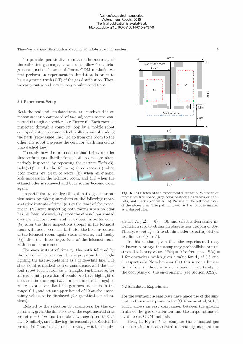
Both the real and simulated tests are conducted in anindoor scenario composed of two adjacent rooms con-

nected through a corridor (see Figure 6). Each room is

inspected through a complete loop by a mobile robot

equipped with an e-nose which collects samples alongthe path (red-dashed line). To go from one room to the

other, the robot traverses the corridor (path marked as

blue-dashed line).

To study how the proposed method behaves under

time-variant gas distributions, both rooms are alter-

natively inspected by repeating the pattern ”left(x3),

right(x1)”, under the following three cases: (i) when

both rooms are clean of odors, (ii) when an ethanolleak appears in the leftmost room, and (iii) when the

ethanol odor is removed and both rooms become clean

again.

In particular, we analyze the estimated gas distribu-

tion maps by taking snapshots at the following repre-

sentative instants of time: (t0) at the start of the exper-

iment, (t1) after inspecting both rooms when no odorhas yet been released, (t2) once the ethanol has spread

over the leftmost room, and it has been inspected once,

(t3) after the three inspections (loops) in the leftmost

room with odor presence, (t4) after the first inspection

of the leftmost room, again clean of odors, and finally(t5) after the three inspections of the leftmost room

with no odor presence.

For each instant of time ti, the path followed bythe robot will be displayed as a grey-thin line, high-

lighting the last seconds of it as a thick-white line. The

start point is marked as a circumference, and the cur-

rent robot localization as a triangle. Furthermore, for

an easier interpretation of results we have highlightedobstacles in the map (walls and office furnishings) in

white color, normalized the gas measurements in the

range [0,1], and set an upper bound of 12 on the uncer-

tainty values to be displayed (for graphical considera-tions).

Related to the selection of parameters, for this ex-

periment, given the dimensions of the experimental area,we set c = 0.5m and the robot average speed to 0.25

m/s. Similarly, and following the reasoning on Section 4.4,

we set the Gaussian sensor noise to σ2s = 0.1, or equiv-

10,4m

10,4m

2,8m

4,75m

0,8m

x3

Corridor path

x1

Non-visited room

(a)

(b)

Fig. 6 (a) Sketch of the experimental scenario. White colorrepresents free space, grey color obstacles as tables or cabi-nets, and black color walls. (b) Picture of the leftmost roomof the above plan. The path followed by the robot is markedas a dashed line.

alently Λok(∆t = 0) = 10, and select a decreasing in-

formation rate to obtain an observation lifespan of 60s.

Finally, we set σ2p = 2 to obtain moderate extrapolation

results (see Figure 5).In this section, given that the experimental map

is known a priory, the occupancy probabilities are re-

stricted to binary values (P (o) = 0 for free space, P (o) =

1 for obstacles), which gives a value for Λp of 0.5 and

0, respectively. Note however that this is not a limita-tion of our method, which can handle uncertainty in

the occupancy of the environment (see Section 3.2.2).

5.2 Simulated Experiment

For the synthetic scenario we have made use of the sim-

ulation framework presented in [G.Monroy et al, 2013],

which allows an easy comparison between the ground

truth of the gas distribution and the maps estimatedby different GDM methods.

First, in Figure 7 we compare the estimated gas

concentration and associated uncertainty maps at the




GMRF GMRF + Obstaclest Ground Truth Estimated Conc. Uncertainty Estimated Conc. Uncertainty

t0

0 2 4 6 8 100

2

4

6

8

10

m

m

0

0.2

0.4

0.6

0.8

1

Cells

Cells

5 10 15 20

2

4

6

8

10

12

14

16

18

20

0

0.2

0.4

0.6

0.8

1

Cells

Cells

5 10 15 20

2

4

6

8

10

12

14

16

18

20

0.5

1

1.5

2

2.5

3

3.5

4

Cells

Cells

5 10 15 20

2

4

6

8

10

12

14

16

18

20

0

0.2

0.4

0.6

0.8

1

Cells

Cells

5 10 15 20

2

4

6

8

10

12

14

16

18

20

2

4

6

8

10

t1

0 2 4 6 8 100

2

4

6

8

10

m

m

0

0.2

0.4

0.6

0.8

1

Cells

Cel

ls

5 10 15 20

2

4

6

8

10

12

14

16

18

20

0

0.2

0.4

0.6

0.8

1

Cells

Cel

ls

5 10 15 20

2

4

6

8

10

12

14

16

18

20

0.5

1

1.5

2

Cells

Cel

ls

5 10 15 20

2

4

6

8

10

12

14

16

18

20

0

0.2

0.4

0.6

0.8

1

Cells

Cel

ls

5 10 15 20

2

4

6

8

10

12

14

16

18

20

2

4

6

8

10

t2

0 2 4 6 8 100

2

4

6

8

10

m

m

0

0.2

0.4

0.6

0.8

1

Cells

Cel

ls

5 10 15 20

2

4

6

8

10

12

14

16

18

20

0

0.2

0.4

0.6

0.8

1

Cells

Cel

ls

5 10 15 20

2

4

6

8

10

12

14

16

18

20

0.5

1

1.5

2

Cells

Cel

ls

5 10 15 20

2

4

6

8

10

12

14

16

18

20

0

0.2

0.4

0.6

0.8

1

Cells

Cel

ls

5 10 15 20

2

4

6

8

10

12

14

16

18

20

2

4

6

8

10

t3

0 2 4 6 8 100

2

4

6

8

10

m

m

0

0.2

0.4

0.6

0.8

1

Cells

Cel

ls

5 10 15 20

2

4

6

8

10

12

14

16

18

20

0

0.2

0.4

0.6

0.8

1

Cells

Cel

ls

5 10 15 20

2

4

6

8

10

12

14

16

18

20

0.5

1

1.5

2

Cells

Cel

ls

5 10 15 20

2

4

6

8

10

12

14

16

18

20

0

0.2

0.4

0.6

0.8

1

Cells

Cel

ls

5 10 15 20

2

4

6

8

10

12

14

16

18

20

2

4

6

8

10

t4

0 2 4 6 8 100

2

4

6

8

10

m

m

0

0.2

0.4

0.6

0.8

1

Cells

Cel

ls

5 10 15 20

2

4

6

8

10

12

14

16

18

20

0

0.2

0.4

0.6

0.8

1

Cells

Cel

ls

5 10 15 20

2

4

6

8

10

12

14

16

18

20

0.5

1

1.5

2

Cells

Cel

ls

5 10 15 20

2

4

6

8

10

12

14

16

18

20

0

0.2

0.4

0.6

0.8

1

Cells

Cel

ls

5 10 15 20

2

4

6

8

10

12

14

16

18

20

2

4

6

8

10

t5

0 2 4 6 8 100

2

4

6

8

10

m

m

0

0.2

0.4

0.6

0.8

1

Cells

Cel

ls

5 10 15 20

2

4

6

8

10

12

14

16

18

20

0

0.2

0.4

0.6

0.8

1

Cells

Cel

ls

5 10 15 20

2

4

6

8

10

12

14

16

18

20

0.5

1

1.5

2

Cells

Cel

ls

5 10 15 20

2

4

6

8

10

12

14

16

18

20

0

0.2

0.4

0.6

0.8

1

Cells

Cel

ls

5 10 15 20

2

4

6

8

10

12

14

16

18

20

2

4

6

8

10

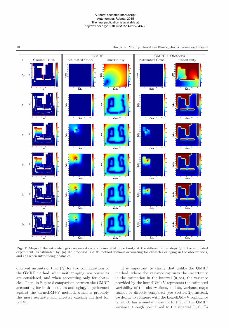
Fig. 7 Maps of the estimated gas concentration and associated uncertainty at the different time steps ti of the simulatedexperiment, as estimated by: (a) the proposed GMRF method without accounting for obstacles or aging in the observations,and (b) when introducing obstacles.

different instants of time (ti) for two configurations ofthe GMRF method: when neither aging, nor obstacles

are considered, and when accounting only for obsta-

cles. Then, in Figure 8 comparison between the GMRF

accounting for both obstacles and aging, is performedagainst the kernelDM+V method, which is probably

the more accurate and effective existing method for

GDM.

It is important to clarify that unlike the GMRFmethod, where the variance captures the uncertainty

in the estimation in the interval (0,∞), the variance

provided by the kernelDM+V represents the estimated

variability of the observations, and so, variance mapscannot be directly compared (see Section 2). Instead,

we decide to compare with the kernelDM+V confidence

α, which has a similar meaning to that of the GMRF

variance, though normalized to the interval [0, 1). To




GMRF+Obstacles+Time kernelDM+Vt Ground Truth Estimated Conc. Uncertainty Mean Confidence

t0

0 2 4 6 8 100

2

4

6

8

10

m

m

0

0.2

0.4

0.6

0.8

1

Cells

Cells

5 10 15 20

2

4

6

8

10

12

14

16

18

20

0

0.2

0.4

0.6

0.8

1

Cells

Cells

5 10 15 20

2

4

6

8

10

12

14

16

18

20

2

4

6

8

10

Cells

Cells

5 10 15 20

2

4

6

8

10

12

14

16

18

20

0

0.2

0.4

0.6

0.8

1

Cells

Cells

5 10 15 20

2

4

6

8

10

12

14

16

18

20

2

4

6

8

10

t1

0 2 4 6 8 100

2

4

6

8

10

m

m

0

0.2

0.4

0.6

0.8

1

Cells

Cel

ls

5 10 15 20

2

4

6

8

10

12

14

16

18

20

0

0.2

0.4

0.6

0.8

1

Cells

Cel

ls

5 10 15 20

2

4

6

8

10

12

14

16

18

20

2

4

6

8

10

Cells

Cel

ls

5 10 15 20

2

4

6

8

10

12

14

16

18

20

0

0.2

0.4

0.6

0.8

1

Cells

Cel

ls

5 10 15 20

2

4

6

8

10

12

14

16

18

20

2

4

6

8

10

t2

0 2 4 6 8 100

2

4

6

8

10

m

m

0

0.2

0.4

0.6

0.8

1

Cells

Cel

ls

5 10 15 20

2

4

6

8

10

12

14

16

18

20

0

0.2

0.4

0.6

0.8

1

Cells

Cel

ls

5 10 15 20

2

4

6

8

10

12

14

16

18

20

2

4

6

8

10

Cells

Cel

ls

5 10 15 20

2

4

6

8

10

12

14

16

18

20

0

0.2

0.4

0.6

0.8

1

Cells

Cel

ls

5 10 15 20

2

4

6

8

10

12

14

16

18

20

2

4

6

8

10

t3

0 2 4 6 8 100

2

4

6

8

10

m

m

0

0.2

0.4

0.6

0.8

1

Cells

Cel

ls

5 10 15 20

2

4

6

8

10

12

14

16

18

20

0

0.2

0.4

0.6

0.8

1

Cells

Cel

ls

5 10 15 20

2

4

6

8

10

12

14

16

18

20

2

4

6

8

10

Cells

Cel

ls

5 10 15 20

2

4

6

8

10

12

14

16

18

20

0

0.2

0.4

0.6

0.8

1

Cells

Cel

ls

5 10 15 20

2

4

6

8

10

12

14

16

18

20

2

4

6

8

10

t4

0 2 4 6 8 100

2

4

6

8

10

m

m

0

0.2

0.4

0.6

0.8

1

Cells

Cel

ls

5 10 15 20

2

4

6

8

10

12

14

16

18

20

0

0.2

0.4

0.6

0.8

1

Cells

Cel

ls

5 10 15 20

2

4

6

8

10

12

14

16

18

20

2

4

6

8

10

Cells

Cel

ls

5 10 15 20

2

4

6

8

10

12

14

16

18

20

0

0.2

0.4

0.6

0.8

1

Cells

Cel

ls

5 10 15 20

2

4

6

8

10

12

14

16

18

20

2

4

6

8

10

t5

0 2 4 6 8 100

2

4

6

8

10

m

m

0

0.2

0.4

0.6

0.8

1

Cells

Cel

ls

5 10 15 20

2

4

6

8

10

12

14

16

18

20

0

0.2

0.4

0.6

0.8

1

Cells

Cel

ls

5 10 15 20

2

4

6

8

10

12

14

16

18

20

2

4

6

8

10

Cells

Cel

ls

5 10 15 20

2

4

6

8

10

12

14

16

18

20

0

0.2

0.4

0.6

0.8

1

Cells

Cel

ls

5 10 15 20

2

4

6

8

10

12

14

16

18

20

2

4

6

8

10

Fig. 8 Maps of the estimated gas concentration and associated uncertainty at the different time steps ti of the simulatedexperiment, as estimated by: (a) the proposed GMRF method accounting for obstacles and observations’s aging (compare theresults with those in Figure 7), and (b) the kernelDM+V method. Notice that for the latter, the transformed confidence valuesare depicted following Eq. (18).

fairly compare both magnitudes, we employ the trans-formation:

σ2i =

1

αi

− 1 (18)

where σ2 represents the corresponding uncertainty val-

ues for the kernelDM+V. To avoid numerical problems

we imposed αi > 0.001.

Although an optimization procedure based on thenegative log predictive density (NLPD) can be used to

select the KernelDM+V parameters when working of-

fline as explained in [Lilienthal et al, 2009], in this work

we need an online comparison, and so, such optimiza-tion cannot be followed. Furthermore, the suggested op-

timization procedure assumes that the gas concentra-

tion is static along the experiment duration, which com-

pletely contradicts our case of study. Instead, we select




its parameters based on the observations found in the

cited paper together with some practical restrictions:

we select the cell size as in our algorithm (c = 0.5m),

and to allow a proper extrapolation of individual read-

ings, we set the kernel width to σ = 0.9m (complyingwith the restriction σ > c). Finally, the cutoff radius

parameter is set to 4σ as proposed in [Lilienthal et al,

2009].

The following conclusions can be drawn from thisexperiment:

1. At time steps t0 (initialization) and t1 (after in-

specting both rooms for the first time), all the com-

pared methods estimate correctly the absence of

volatiles in the environment as appreciated in theirrespective concentration maps. However, their un-

certainty maps differ considerably. The most notice-

able difference is appreciated when introducing the

obstacles in the environment, influencing the corre-

lation between map cells, and consequently the un-certainty maps. Under these circumstances the pro-

posed GMRF method provides low uncertainties for

the visited cells, while for those falling on obstacles

or in non-visited rooms (as the isolated room at thetop left of the map), still maintain high values, as

desired. This contribution enables a better compre-

hension of the estimated maps, since the structure

of the environment (rooms, corridor, walls, etc) is

easily appreciated.2. Once the gas is released, we take snapshots at two

time instants: t2 after only one loop through the

contaminated area, and t3 after three loops, as dis-

played in Figure 6. Here, since both the KernelDM+Vas well as the limited configurations of GMRF and

GMRF+Obstacles do not consider the time at which

observations are taken, the estimated concentration

maps are the result of averaging recent observations

with older ones, that is, with observations gatheredwhen no gas was still released. Notice how at such

time instants, those methods fail to detect the high

concentration values present in the ground truth

maps. This, which represents one of the main lim-itations of existing GDM methods, is successfully

overcome by the proposed approach, as appreciated

in the GMRF+Obstacles+Time maps in Figure 8.

By increasing the uncertainty of observations as they

become older, together with the fact that we con-sider the presence of obstacles in the environment,

our approach is able to detect and correctly localize

the high gas emissions with only one lap over the

contaminated zone. The main difference betweentime-instants t2 and t3, is that at t3 the uncertain-

ties at the right room start increasing as a conse-

quence of the rise in the variance of observations,

t0 t1 t2 t3 t4 t50

0.01

0.02

0.03

0.04

0.05

0.06

0.07

MS

E

Time Step

GMRFGMRF+ObsGMRF+Obs+TimeKernelDM+V: σ = 0.9KernelDM+V: σ = 0.5

Fig. 9 Mean squared error (MSE) at the different time steps(ti) of the simulated experiment, for the KernelDM+V andthe different configurations of the GMRF method.

which allows the method to remove them from the

set of observations.3. Finally, at time steps t4 and t5, when the gas has

been removed, the ”average” effect of methods not

considering the age of observations can still be ap-

preciated as gas patches in the concentration maps.On the contrary, our approach adapts faster to chang-

ing gas concentrations, and so it correctly provides a

zero concentration estimation at the left room, even

after only one lap (t4).

To quantitatively compare the different configura-

tions of the proposed GMRF method, among them-

selves, and with other methods previously proposed inthe literature, we employ the mean squared error per-

formance measure (MSE). The MSE is calculated as

the difference between the ground-truth concentration

ci and the estimated MAP value mi, or the mean valueµi for the kernelDM+V method.

MSE =1

N

N∑

i=1

(ci −mi))2 (19)

Figure 9 shows the MSE for the different time steps(ti) of the simulation. Since the kernelDM+V perfor-

mance is dependent of the kernel size, we also include

the performance measures of or a reduced kernel size of

σ = 0.5, which corresponds to the smaller kernel sizegiven the selected cell size in the experiment. As can

be appreciated, our approach introduces a notable im-

provement, being remarkable the inclusion of obstacles

in the GDM process.

A particular case is the comparison between the

simplest GMRF configuration and the kernelDM+V,

showing both similar performance measures (even ad-

vantageous for the kernelDM+V when considering thereduced kernel size). This unveils the importance of con-

sidering obstacles and observation ageing in the GDM

process, which not only reduce considerably the MSE




on the estimated gas concentration, but also provide

more realistic uncertainty maps.

Other performance measures which not only account

for the estimated concentration values, but also con-

sider the uncertainty on the estimation (e.g the NLPD),

have not been considered in this work because of theinherent differences in the variances of the compared

methods. While for the kernelDM+V the variance rep-

resents the estimated variability of the gas observations,

for the proposed GMRF method the variance repre-

sents the uncertainty about the estimated gas concen-tration, and thus, to the best knowledge of the authors,

they cannot be compared. Similarly, kernelDM+V con-

fidence values α, which have been used in the graphical

comparison because of the likeness with the uncertaintyof the estimations, can neither be used to compute per-

formance measures such as the NLPD because they are

not strictly variances, and so, a quantitatively compar-

ison would be meaningless.

5.3 Real Experiment

Following the same setup than in the simulated exper-

iment, we show next the results of a real experience.In this case the gas observations are collected with a

photo ionization detector (PID2), mounted in a Patrol-

Bot [MobileRobots Inc., 2014] mobile platform. To al-

low comparison with the results of the simulated ex-

periment, the ppm readings provided by the PID arenormalized to the range [0,1].

To generate the gas leak in the left room, we place

an ethanol bottle in front of a fan to boost the gas

dispersion. The ethanol bottle was timely opened or

closed to match the setup described in Section 5.1. This

configuration generates a gas plume towards the doorheading to the corridor when the ethanol bottle is open,

while it helps cleaning the room from gases when the

bottle is closed.

In this case, only the full configuration of the pro-

posed GMRF is compared to the kernelDM+V. For a

fair comparison among them, the experimental data iscollected and saved to a log file for off-line processing.

In this way, differences from both estimations will only

obey to differences in the methods and not to the data.

Figure 10 shows the estimated concentration and

uncertainty maps generated by the GMRF and the Ker-

nelDM+V. As in the simulation experiment, snapshotsof the maps at the different time steps (ti) are depicted.

Since the ground truth of the gas distribution is not

2 Model ppbRAE2000 from RAESystem, with a 10.6 eVUV lamp.

available, we plot instead the obstacles map together

with the robot localization.

As can be noticed, the results are quite similar to

those obtained in simulation, which corroborates the al-ready highlighted advantages of our proposal. The main

difference resides in the presence of low concentration

gases in the left room at time steps t4 and t5, after the

ethanol bottle is closed. This can be attributed to the

fact that the time elapsed since the ethanol bottle wasclosed till the robot inspected back the room, was not

enough for the gas to disappear.

5.4 Execution Time

Finally, we compare the execution time of the differ-

ent configurations of the GMRF method and the ker-nelDM+V for different map sizes. This is done by con-

sidering the same experimental setup as described in

Section 5.1, but reducing the cell size to increase the

overall number of cells in the map. Figure 11 summa-rizes this comparison, plotting the execution time cor-

responding to the resolution of the least-squares prob-

lem together with the recovery of the associated un-

certainty (see Section 4.3). As can be appreciated, the

computational cost of the kernelDM+V method is al-most independent of the map size, and in the order of

few milliseconds. This is because the number of cells to

be updated for each new gas observation is trunked by

the cutoff radius parameter, keeping almost constantthe execution time. Conversely, the GMRF method is

strongly dependent of the map size, updating all map

cells at each time step in order to reflect the effect of

obstacles and observation aging.

An interesting property shared by both methods isthe fact that they allow batch of observations. This

is specially important for the GMRF method, mean-

ing that we are not forced to execute the algorithm

for each new gas observation, but we can stock obser-vations for few milliseconds or even seconds and then

update the map maintaining the same execution time

as in the case of considering only one observation at

a time. An example of this property can be observed

when comparing the execution time of GMRF+Obs andGMRF+Obs+Time. The main difference between these

configurations is that the latter works only with a fi-

nite set of M observations from the set of all observa-

tions (the most recent ones), yet their execution timesare almost identical. This property allows the proposed

GMRF method to be used online even for big map sizes,

although reducing the updating frequency.




GMRF+Obs+Time Kernel DM+Vt Obstacles Map Estimated Conc. Uncertainty Mean Confidence

t0

−8 −6 −4 −2 0 2 4

8

6

4

2

0

−2

m

m

0.1

0.2

0.3

0.4

0.5

0.6

0.7

0.8

0.9

Cells

Cells

5 10 15 20

5

10

15

20

25

0

02

0

0�

0�

1

Cells

Cells

5 10 15 20

5

10

15

20

25

2

4

6

8

10

Cells

Cells

5 10 15 20

5

10

15

20

25

0

0�2

0��

0��

0��

1

Cells

Cells

5 10 15 20

5

10

15

20

25

2

4

6

8

10

t1

−8 −6 −4 −2 0 2 4

8

6

4

2

0

−2

m

m

0.1

0.2

0.3

0.4

0.5

0.6

0.7

0.8

0.9

Cells

Cel

ls

5 10 15 20

5

10

15

20

25

0

0.2

0.4

0.6

0.8

1

Cells

Cel

ls

5 10 15 20

5

10

15

20

25

2

4

6

8

10

Cells

Cel

ls

5 10 15 20

5

10

15

20

25

0

0.2

0.4

0.6

0.8

1

Cells

Cel

ls

5 10 15 20

5

10

15

20

25

2

4

6

8

10

t2

−8 −6 −4 −2 0 2 4

8

6

4

2

0

−2

m

m

0.1

0.2

0.3

0.4

0.5

0.6

0.7

0.8

0.9

Cells

Cel

ls

5 10 15 20

5

10

15

20

25

0

0.2

0.4

0.6

0.8

1

Cells

Cel

ls

5 10 15 20

5

10

15

20

25

2

4

6

8

10

Cells

Cel

ls

5 10 15 20

5

10

15

20

25

0

0.2

0.4

0.6

0.8

1

Cells

Cel

ls

5 10 15 20

5

10

15

20

25

2

4

6

8

10

t3

−8 −6 −4 −2 0 2 4

8

6

4

2

0

−2

m

m

0.1

0.2

0.3

0.4

0.5

0.6

0.7

0.8

0.9

Cells

Cel

ls

5 10 15 20

5

10

15

20

25

0

0.2

0.4

0.6

0.8

1

Cells

Cel

ls

5 10 15 20

5

10

15

20

25

2

4

6

8

10

Cells

Cel

ls

5 10 15 20

5

10

15

20

25

0

0.2

0.4

0.6

0.8

1

Cells

Cel

ls

5 10 15 20

5

10

15

20

25

2

4

6

8

10

t4

−8 −6 −4 −2 0 2 4

8

6

4

2

0

−2

m

m

0.1

0.2

0.3

0.4

0.5

0.6

0.7

0.8

0.9

Cells

Cel

ls

5 10 15 20

5

10

15

20

25

0

0.2

0.4

0.6

0.8

1

Cells

Cel

ls

5 10 15 20

5

10

15

20

25

2

4

6

8

10

Cells

Cel

ls

5 10 15 20

5

10

15

20

25

0

0.2

0.4

0.6

0.8

1

Cells

Cel

ls

5 10 15 20

5

10

15

20

25

2

4

6

8

10

t5

−8 −6 −4 −2 0 2 4

8

6

4

2

0

−2

m

m

0.1

0.2

0.3

0.4

0.5

0.6

0.7

0.8

0.9

Cells

Cel

ls

5 10 15 20

5

10

15

20

25

0

0.2

0.4

0.6

0.8

1

Cells

Cel

ls

5 10 15 20

5

10

15

20

25

2

4

6

8

10

Cells

Cel

ls

5 10 15 20

5

10

15

20

25

0

0.2

0.4

0.6

0.8

1

Cells

Cel

ls

5 10 15 20

5

10

15

20

25

2

4

6

8

10

Fig. 10 Maps of the estimated gas concentration and associated uncertainty at the different time steps ti of the real experiment,as estimated by: (a) the proposed GMRF method accounting for obstacles and observations’s aging, and (b) the kernelDM+Vmethod. Notice that for the latter, the transformed confidence values are depicted following Eq. (18).

6 Conclusions and Future Work

In this paper we have revised the problem of creat-

ing a map of the gas distribution and proposed a new

approach that accounts for two important issues that

had been ignored in previous works: the aging of theobservations and the presence of obstacles in the en-

vironment. The former is achieved by introducing a

time-decreasing weighting factor to each gas observa-

tion. Thus, when combining observations taken at close

locations, their ages are used to determine their rele-vances, avoiding the detrimental ”average” effect of pre-

vious approaches. On the other hand, obstacles such as

walls or furniture are now taken into account by model-

ing the correlation between the map cells they separate.

We have addressed the problem in a probabilistic man-ner modeling the problem as a MAP estimation over a

Gaussian Markov random field (GMRF).




0 500 1000 1500 2000 2500 30000

500

1000

1500

2000

Exe

cutio

n tim

es (

ms)

Map size (cells)

GMRFGMRF+ObsGMRF+Obs+TimekernelDM+V

Fig. 11 Execution time for the different configurations ofthe GMRF method and the kernelDM+V, for different mapsizes.

Our approach has been validated with simulated

and real experiments, providing qualitative and quan-

titative comparison with classical methods and demon-

strating the advantages in the estimation of the gasdistribution.

Future work includes the consideration of additional

sources of information such as vision or semantics to

improve the way cell correlations are modeled, exploit-

ing properties of the obstacles that influence the gasdispersion (shape, height, etc). Furthermore, efficient

alternatives to obtain the GDM of non rectangular sce-

narios will be studied, for example, by only estimating

the gas concentration at desired areas instead of thecomplete rectangular lattice.

Acknowledgements

The authors would like to thank Achim J. Lilienthal

and Sahar Asadi for the fruitful discussions about ker-nel methods for gas distribution mapping.

Funding

This work was supported by the Andalucıa RegionalGovernment and the European Union (FEDER) [TEP08-

4016]; and by the Spanish ”Ministerio de Ciencia e In-

novacion” and the grant program JDC-MICINN 2011

[DPI2011-25483].

References

Airsense Analytics (2014) PEN3.

http://www.airsense.com/en/products/pen3/

Asadi S, Pashami S, Loutfi A, Lilienthal AJ (2011)Td kernel dm+v: Time-dependent statistical gas dis-

tribution modelling on simulated measurements. In:

Proceedings of the 14th International Symposium on

Olfaction and Electronic Nose (ISOEN), vol 1362, pp

281–283

Bishop CM (2007) Pattern Recognition and Machine

Learning. Springer

Bjorck A (1996) Numerical methods for least squaresproblems. Society for Industrial and Applied Mathe-

matics

Blanco JL, Gonzalez-Jimenez J, Fernandez-Madrigal

JA (2010) Optimal filtering for non-parametricobservation models: Applications to localiza-

tion and SLAM. The International Journal

of Robotics Research 29(14):1726–1742, DOI

10.1177/0278364910364165

Blanco JL, G Monroy J, Gonzalez-Jimenez J, Lilien-thal AJ (2013) A kalman filter based approach to

probabilistic gas distribution mapping. In: 28th Sym-

posium On Applied Computing (SAC), pp 217–222,

DOI 10.1145/2480362.2480409Clifford P (1990) Markov random fields in statistics. In:

Grimmett G, Welsh D (eds) Disorder in Physical Sys-

tems: A Volume in Honour of John M. Hammersley,

Oxford University Press, Oxford, pp 19–32

Davis TA (2004) A column pre-ordering strategyfor the unsymmetric-pattern multifrontal method.

ACM Trans Math Softw 30(2):165–195, DOI

10.1145/992200.992205

Dellaert F, Kaess M (2006) Square root sam: Simulta-neous localization and mapping via square root in-

formation smoothing. The International Journal of

Robotics Research 25(12):1181–1203

Dennis J, Schnabel R (1983) Numerical Methods for

Unconstrained Optimization and Nonlinear Equa-tions. Classics in Applied Mathematics, Society for

Industrial and Applied Mathematics

Fenger J (1999) Urban air quality - their physi-

cal and chemical characteristics. Atmospheric Envi-ronment 33(29):4877–4900, DOI doi:10.1016/S1352-

2310(99)00290-3

Fernandez-Madrigal JA, Blanco JL (2013) Simultane-

ous Localization and Mapping for Mobile Robots: In-

troduction and Methods. Information Science Refer-ence

Frish MB, Wainner RT, Green BD, Laderer MC,

Allen MG (2005) Standoff gas leak detectors based

on tunable diode laser absorption spectroscopy.In: Proc. SPIE 6010, Infrared to Terahertz Tech-

nologies for Health and the Environment, DOI

10.1117/12.630599

G Monroy J, Gonzalez-Jimenez J, Blanco JL (2012)

Overcoming the slow recovery of mox gas sen-sors through a system modeling approach. Sensors

12(10):13,664–13,680, DOI 10.3390/s121013664




GMonroy J, Blanco JL, Gonzalez-Jimenez J (2013)

An open source framework for simulating mobile

robotics olfaction. In: Proceedings of the 15th In-

ternational Symposium On Olfaction and Electronic

Nose (ISOEN)Golub GH, Plemmons RJ (1980) Large-scale geodetic

least-squares adjustment by dissection and orthogo-

nal decomposition. Linear Algebra and its Applica-

tions 34(0):3 – 28, DOI 10.1016/0024-3795(80)90156-1

Gonzalez-Jimenez J, G Monroy J, Blanco JL

(2011) The multi-chamber electronic nose. an im-

proved olfaction sensor for mobile robotics. Sensors

11(6):6145–6164, DOI 10.3390/s110606145Ishida H, Ushiku T, Toyama S, Taniguchi H, Moriizumi

T (2005) Mobile robot path planning using vision and

olfaction to search for a gas source. In: IEEE Sensors,

DOI 10.1109/ICSENS.2005.1597899Lilienthal AJ, Duckett T (2004) Building gas concen-

tration gridmaps with a mobile robot. Robotics and

Autonomous Systems 48(1):3–16

Lilienthal AJ, Loutfi A, Blanco JL, Galindo C,

Gonzalez-Jimenez J (2007) A rao-blackwellisationapproach to GDM-SLAM: Integrating SLAM and gas

distribution mapping (GDM). In: 3rd European Con-

ference on Mobile Robots (ECMR)

Lilienthal AJ, Reggente M, Trincavelli M, BlancoJL, Gonzalez-Jimenez J (2009) A statistical ap-

proach to gas distribution modelling with mo-

bile robots - the kernel dm+v algorithm. In:

IEEE/RSJ International Conference on Intelligent

Robots and Systems, IROS., pp 570 –576, DOI10.1109/IROS.2009.5354304

Loeliger HA (2004) An introduction to factor graphs.

IEEE Signal Processing Magazine 21(1):28–41, DOI

10.1109/MSP.2004.1267047Loufti A, Coradeschi S, Lilienthal AJ, Gonzalez-

Jimenez J (2009) Gas distribution mapping of mul-

tiple odour sources using a mobile robot. Robotica

27:311–319, DOI 10.1017/S0263574708004694

Madsen K, Nielsen HB, Tingleff O (2004) Methods fornon-linear least squares problems (2nd ed.)

Marjovi A, Marques L (2013) Optimal spatial forma-

tion of swarm robotic gas sensors in odor plume

finding. Autonomous Robots 35(2-3):93–109, DOI10.1007/s10514-013-9336-1

MobileRobots Inc (2014) Corporate website.

http://www.mobilerobots.com

Pashami S, Asadi S, Lilienthal AJ (2010) Integration

of openfoam flow simulation and filament-based gaspropagation models for gas dispersion simulation. In:

Proceedings of the Open Source CFD International

Conference

Reggente M, Lilienthal AJ (2009) Three-dimensional

statistical gas distribution mapping in an uncon-

trolled indoor environment. In: Proceedings of the

13th International Symposium on Olfaction and Elec-

tronic Nose (ISOEN), vol 1137, pp 109–112Sanchez-Garrido C, G Monroy J, Gonzalez-Jimenez

J (2014) A configurable smart e-nose for spatio-

temporal olfactory analysis. In: IEEE Sensors, pp

1968–1971, DOI 10.1109/ICSENS.2014.6985418Sensigent Intelligent Sensing So-

lutions (2014) Cyranose 320.

http://www.sensigent.com/products/cyranose.html

Shraiman BI, Siggia ED (2000) Scalar turbulence. Na-

ture 405:639–646, DOI 10.1038/35015000Stachniss C, Plagemann C, Lilienthal AJ (2009) Gas

distribution modeling using sparse gaussian process

mixtures. Autonomous Robots 26(2-3):187–202

Tauseef S, Rashtchian D, Abbasi S (2011) Cfd-based simulation of dense gas dispersion in pres-

ence of obstacles. Journal of Loss Prevention in

the Process Industries 24(4):371 – 376, DOI

10.1016/j.jlp.2011.01.014

Trincavelli M, Hernandez Bennetts V, LilienthalAJ (2012) A least squares approach for learn-

ing gas distribution maps from a set of integral

gas concentration measurements obtained with a

tdlas sensor. In: IEEE Sensors, pp 1–4, DOI10.1109/ICSENS.2012.6411118

Tsujita W, Yoshino A, Ishida H, Moriizumi T (2005)

Gas sensor network for air-pollution monitoring. Sen-

sors and Actuators B: Chemical 110(2):304 – 311,

DOI 10.1016/j.snb.2005.02.008Turduev M, Cabrita G, Kırtay M, Gazi V, Marques L

(2014) Experimental studies on chemical concentra-

tion map building by a multi-robot system using bio-

inspired algorithms. Autonomous Agents and Multi-Agent Systems 28(1):72–100, DOI 10.1007/s10458-

012-9213-x

Winkler G (2003) Image analysis, random fields and

Markov chain Monte Carlo methods: a mathematical

introduction, vol 27. Springer Verlag



Documents

Time-VariantGas DistributionMapping withObstacleInformationingmec.ual.es/~jlblanco/papers/2015_GDM_TimeVariant_Obstacles... · Time-VariantGas DistributionMapping withObstacleInformation