Time to Dropout from College: A Hazard Model with Endogenous Waiting*

Dennis A. Ahlburg, Brian P. McCall,

In-gang NaIndustrial Relations Center

University of Minnesotarevised April 2002

* We thank Steve DesJardins, Audrey Light and seminar participants at New York

University, University of Chicago, University of Kentucky, University of Melbourne,

and University of New South Wales for helpful comments and the Minnesota

Supercomputer Institute for support in the form of a resource grant.

Abstract

Using data from the 1979 National Longitudinal Survey of Youth (NLSY79), we

investigate the college attendance, dropout and graduate behavior of high school graduates.

Bivariate duration models, which allow the unobserved determinants of spell durations to

be correlated across spells, are developed and used to study the impact of the waiting

time from high school graduation until college enrollment on college dropout and

graduation rates. We find that delaying college entry after graduating high school

significantly increases the chances of college dropout and reduces the probability of

attaining a four year degree. Among those who first enroll in four-year institutions,

delaying college entry by one year after high school graduation reduces the probability of

graduating with a four-year degree by up to 32 percent in models that account for the

endogeneity of delaying enrollment. There is also empirical evidence that the negative

impact of delayed enrollment on graduation probabilities varies by Armed Forces

Qualifying Test (AFQT) score with the largest estimated impact of delaying occurring for

those with low AFQT scores.

1

1. Introduction

A recent story in the New York Times discussed a “small but apparently growing

number of high achieving, well-off students [who] are stepping off the fast educational

track, at least for a short stroll” (New York Times 2001:A1. A17). The story reported

that guidance counselors and college admissions officers along with a flourishing industry

of consultants are promoting the notion that “higher education works best for those who

wait” (New York Times 2001:A17). Although some individuals may benefit from

delaying entry to college is this true for students in general? Before rushing to advise

students to take a year off before attending college, we need to know what impact this

will have on their chances of graduating.

Delaying entry to college is not a new phenomenon. Among the high school

graduating classes of 1972, 1980, and 1982 about one-quarter of those who entered post-

secondary education within four years of graduating from high school delayed entry.

One-third of those who delayed entry delayed by more than two years. Fourteen years

after high school graduation, 68 percent of the class of 1972 had enrolled in some form of

post-secondary education and almost one-third had delayed entry (Eagle and Carroll

1988). An analysis of the high school graduating class of 1980 revealed that 53 percent of

those who started a bachelor’s degree “on-track” subsequently obtained a degree. In

comparison, only 21 percent of those who delayed entry graduated. The effects of delay

vary across individuals. For example, when high socioeconomic status students delay

1A similar conclusion can be drawn from the recent analysis of the High School and Beyond/Sophomore

1982 cohort. Fully 51 percent of those who did not delay entry to college earned a bachelor’s degree whileonly 20 percent of those who delayed seven to 18 months and ten percent of those who delayed more than18 months earned a bachelor’s degree (Adelman 1999:45).

2

entry, 34 percent eventually graduate whereas only 8 percent of low socioeconomic

status students who delayed graduated. These findings led the Department of Education

researchers to conclude:” knowing that a decision to delay entry…can mean the chances

of getting a bachelor’s degree are five times lower than they would be if the student

started on track should result in better decisions by high school seniors.” (US Department

of Education 1989:29).1

The data from the Department of Education suggests caution before

recommending a year off before college. An additional reason for institutions to be

concerned about students delaying entry is that there is a growing use of institutional

graduation rates as a measure of accountability and a tendency to blame colleges for the

failure of students to graduate or to graduate in a timely manner (Adelman 1999).

The college wage premium rose to an unprecedented level in the 1980’s (Bound

and Johnson, 1989; Murphy and Welch, 1993; Brewer, Eide, and Ehrenberg, 1999).

College graduates have twice the earnings and two and one- half times the wealth of high

school graduates.(Diaz-Gimenz, Quadrini, and Rios-Rull, 1997). Thus, to the extent that

delaying college attendance after graduating high school lowers the amount of post-

3

secondary schooling a high school graduate receives, delay can be costly in terms of

reduced future earnings.

This paper investigates the determinants of college completion and dropout and,

in particular, the impact of delayed entry on college completion and dropout. It expands

upon the existing research tradition by specifying the duration of college attendance until

exit as influenced by an endogenous waiting duration until college enrollment (the delay

between first college enrollment and high school graduation), family background, personal

characteristics, and local labor market conditions. The aim of this paper is to identify the

effect of these covariates on college duration, that is, time to graduation and dropout.

To estimate the determinants of the duration of college attendance, while

accounting for the effect of the (possibly) endogenous waiting time until enrollment, two

bivariate discrete-time hazard models with competing risks are estimated. In the first, we

jointly model the duration until college enrollment and the duration of college attendance

until exit. For the duration until college enrollment, no distinction is made between those

who enroll in a two-year versus four year institutions, since some of those who initially

enroll in a two-year institution may ultimately attain a four-year degree. Thus, the

standard discrete-time hazard approach is used to model this duration (Kiefer, 1988, Han

and Hausman, 1990; Meyer, 1990). In the empirical model we allow college exit to occur

for two reasons: dropout and graduation. Thus, the duration of college attendance is

4

modeled using a discrete-time competing risks approach (see McCall, 1996, for example).

To allow for the possible endogeneity of the waiting time until college enrollment, the

unobservable determinants of the waiting duration until enrollment are allowed to be

correlated with the unobservable determinants of the dropout and graduation risks.

In the second model, we explicitly distinguish between those who first enroll in a

two-year institution and those who first enroll in a four-year institution using a

competing risks approach. Thus, we model both durations as competing risks. Moreover,

when analyzing the enrollment duration we estimate separate competing risks models for

those who enter two-year institutions and for those who enter four-year institutions.

Again, to account for the possibility of endogeneity of waiting time until enrollment, the

unobservable determinants of the risks are allowed to be correlated both within and across

the waiting time and college attendance durations.

After a brief (and selective) review of previous research findings in Section 2,

Section 3 describes the empirical methods employed in this paper. The 1979 National

Longitudinal Survey of Youth data are described in Section 4. Section 5 presents the

empirical findings. Even after controlling for potential endogeneity, waiting time until

college enrollment is found to be an important determinant of college completion. For

example, we find that those who delay enrollment into a four-year institution by one year

decrease their probability of graduating with a four year degree by up to 32 percent.

5

Moreover, we find evidence that suggests that delayed enrollment leads to a larger

reduction in the probability of college graduation for those who score lower on the Armed

Forces Qualifying Test (AFQT). The final section contains a summary and conclusions.

2. Studies of Educational Attainment

Family background variables such as educational attainment and occupations of

parents, family income, and number of siblings are commonly used as control variables in

the study of educational attainment. These family background variables, which appear in

the educational attainment literature, are primarily intended to capture the financial

resources available to students (Light, 1995b). Higher family income is assumed to

increase the likelihood of college enrollment and college graduation, or decrease the

likelihood of college dropout, other things being equal. The number of siblings also affects

educational attainment in the sense that the presence of siblings represents a competing

use of family resources. The educational levels and occupations of parents capture not

only the effect of family resources but also the positive correlations in educational

attainment across generations. These correlations across generations may result from

correlations between educational attainment and family income or from the effect of

educational levels and occupations of parents on youths’ aspirations and the degree of

family support or encouragement to successfully complete college.

6

Empirical studies have found strong positive effects of family background

variables on educational attainment. Family socioeconomic status, operationalized by

educational levels or occupation of parents, family income, or some combinations of these

is found to increase (decrease) the likelihood of college enrollment and college graduation

(college dropout) (Manski and Wise, 1983; Manski, 1989; McLanahan, 1985; NCES,

1989; Kane, 1994). These findings demonstrate the significant influence of family

backgrounds in determining youths’ educational attainment.

Unlike in the study of high school dropout, there is relatively little of empirical

study on the effect of local labor market conditions on college enrollment and college

dropout. In one of the few studies, Kane (1994) found that unemployment rates were not

related to individual enrollment decisions for blacks or whites.

The decision whether or not to attend college is made with imperfect information

(see Manski, 1989; Altonji, 1993). Thus, individuals may dropout of college if they

subsequently learn after enrolling that the “costs” of schooling are higher than they

expected. Also, individuals who do not enroll in college immediately after high school

graduation may subsequently enroll if the subsequently learn they are ill-suited to

occupations that require only a high school education (see Miller, 1984; McCall, 1990;

and Neal, 1999).

2 See Chapter 2 in Tinto (1993) for more detailed definitions.

7

In the classic research on college degree attainment, three categories of college

students were distinguished (Tinto, 1988, 1993; NCES, 1989): persisters, stopouts, and

dropouts. Persisters were defined as students who continued toward their degree goals;

stopouts withdrew and subsequently returned; and dropouts withdrew and never

returned.2

However, there are several reasons for expanding upon these definitions. First,

students may not only stop out and drop out, they may delay entry, enroll part-time,

and transfer between institutions (see Adelman, 1999). These behaviors require a more

complete set of behavioral definitions. Second, definitions of stopouts and dropouts are

directly related to the survey follow-up periods. For example, the National Center for

Education Statistics (NCES, 1989) defined dropouts as those who never return to

complete bachelor’s degree by the last survey year. For the class of 1980, it was by

February of 1986. Thus, the classification of a dropout or stopout can depend on the

length of follow-up periods. Third, another issue related to dropout is the need to

distinguish between dropout from a specific institution and that from the higher education

system as a whole. From the perspective of an institution, it can be reasonably argued

that all students who leave can be classified as dropouts regardless of their reasons. From

the perspective of the higher education system, this may not be the case. That is, a

3 In case of high school dropout, five different definitions of dropout are used in the various studies. seeKominski (1990).

8

student who leaves one institution but enrolls in another institution is an institutional-

dropout but not a system-dropout. Consequently, there is no universally accepted

definition of dropout or stopout.3

In this paper, the following definition of dropout is used: a “dropout” is a student

who left college and did not return to any institution in the higher education system by

the end of the survey period (Fall 1990 in the NLSY 79 data). Under this definition, there

are two reasons for exit from college: graduation or dropout. The graduation group is

defined as those who graduated with a 4-year college degree. Some of them may have

experienced stopout periods during their college career.

3. A Competing Risks Model with Endogenous Waiting time

We consider the case where an individual experiences two distinct durations. The

first duration is the delay time between high school graduation and college enrollment.

The second duration is the duration of college attendance, which may depend on the delay

time between high school graduation and enrollment. Since educational duration data in the

NLSY are measured in years, a discrete-time hazard approach is taken (see Kiefer, 1988;

Meyer, 1990; and Narendranathan and Stewart, 1990 , for example). Moreover, the

9

college attendance duration can end either because the individual drops out of college or

because they graduate from college. Thus, for the second duration we take a competing

risks approach (see Katz, 1986, Hausman and Han, 1990; Anderson, 1992; Sueyoshi,

1992; and McCall, 1996, for example).

Let Tf be the waiting time between high school graduation and college enrollment.

Let Tg be the duration of college attendance until graduation (graduation duration) and let

Td be the duration of college attendance until dropout (dropout duration). Further, let Ts

= min(Tg, Td).

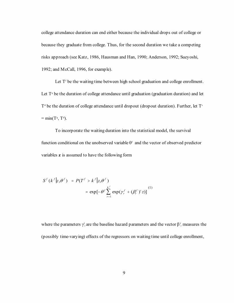
To incorporate the waiting duration into the statistical model, the survival

function conditional on the unobserved variable θf and the vector of observed predictor

variables z is assumed to have the following form

S k z P T k z

z

f f f f f f

frf

r

k

rf

f

( , ) ( , )

exp[ exp( ( ) )]

θ θ

θ γ β

= >

= − + ′=∑

1

(1)

where the parameters γfr are the baseline hazard parameters and the vector βf

r measures the

(possibly time-varying) effects of the regressors on waiting time until college enrollment,

4For simplicity of notation, the regressors are assumed to be time-constant. The model is easily extendedto the case of time-varying regressors although the notation is cumbersome.

10

S k k x T x T

x T

g d g d f grg

rg

rg f

r

k

drd

rd

rd f

r

k

g

d

( , , , , ) exp[ exp( ( ) )

exp( ( ) )]

θ θ θ γ β α

θ γ β α

= − + ′ +

− + ′ +

=

=

∑

∑

1

1

(2)

r= 1, 2, 3, þ.4 Further, it is assumed that θf is distributed independently of the vector of

predictor variables z.

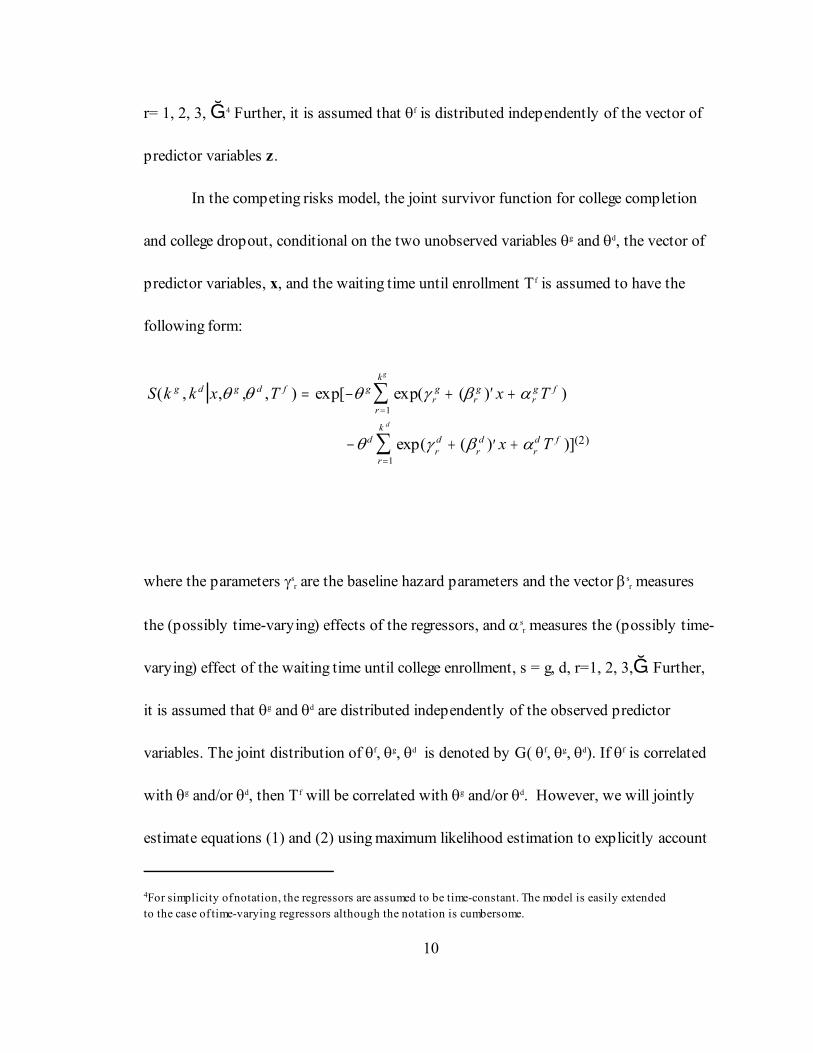
In the competing risks model, the joint survivor function for college completion

and college dropout, conditional on the two unobserved variables θg and θd, the vector of

predictor variables, x, and the waiting time until enrollment Tf is assumed to have the

following form:

where the parameters γsr are the baseline hazard parameters and the vector βs

r measures

the (possibly time-varying) effects of the regressors, and αsr measures the (possibly time-

varying) effect of the waiting time until college enrollment, s = g, d, r=1, 2, 3,þ. Further,

it is assumed that θg and θd are distributed independently of the observed predictor

variables. The joint distribution of θf, θg, θd is denoted by G( θf, θg, θd). If θf is correlated

with θg and/or θd, then Tf will be correlated with θg and/or θd. However, we will jointly

estimate equations (1) and (2) using maximum likelihood estimation to explicitly account

11

pnn

N

=∑ =

11

for the possibility of endogeneity. It is assumed that G has a point-mass structure. In

particular, we assume that there are N triplets of “location” parameters (θf, θg, θd) in the

population where each triplet (θf, θg, θd)n occurs with proportion pn:

Controlling for unobserved heterogeneity is important in models of educational

attainment to mitigate potential selection bias (Willis and Rosen, 1979; Cameron and

Heckman,1998). The likelihood function associated with this duration - competing risks

(DCR) model is derived in the appendix.

High school graduates attending college may enroll in either two-year or four-year

institutions. Some individuals who complete a two-year degree may then continue on to

get a four-year degree. In equation (2) above, one predictor variable that included in the

specifications will indicate whether the individual first entered a two-year versus a four-

year institution. Moreover, we allow for the coefficient associated with this predictor

variable to be time-varying in both the college completion and dropout risks.

Alternatively, we model the duration until college enrollment as ending because

of two reasons: entry into a two-year institution or entry into a four-year institution.

Thus, we take a competing risks approach where Tf = min(T2y, T4y) and T2yand T4y

5The likelihood function for the CR2 model can be derived in a manner similar to that for the DCR model(see Appendix B). For the sake of brevity, however, we omit its derivation in this paper.

12

S k k z z

z

y y y y yr

yr

y

r

k

ry

ry

r

k

y

y

( , , , ) exp[ exp( ( ) )

exp( ( ) )]

2 4 2 4 2 2 2

1

4 4

1

2

4

θ θ θ γ β

γ β

= − + ′

− + ′

=

=

∑

∑(1')

pnn

N

=∑ =

11.

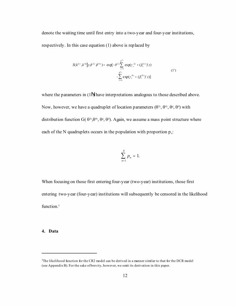
denote the waiting time until first entry into a two-year and four-year institutions,

respectively. In this case equation (1) above is replaced by

where the parameters in (1N) have interpretations analogous to those described above.

Now, however, we have a quadruplet of location parameters (θ2y, θ4y, θg, θd) with

distribution function G( θ2y,θ4y, θg, θd). Again, we assume a mass point structure where

each of the N quadruplets occurs in the population with proportion pn:

When focusing on those first entering four-year (two-year) institutions, those first

entering two-year (four-year) institutions will subsequently be censored in the likelihood

function.5

4. Data

6Source of state tuition data is State Comparisons of Education Statistics: 1969-70 to 1996-97, NationalCenter for Education Statistics.

13

The data for this study come from the 1979 National Longitudinal Survey of

Youth (NLSY79), an ongoing study of 12,686 young individuals who were aged 14 to 21

as of January 1, 1979. The NLSY79 includes information on college attendance, type of

college (two-year versus four-year college) as well as personal characteristics such as age,

sex, race, number of siblings, Armed Forces Qualifying Test (AFQT) score, and

information on the education levels and occupations of parents.

We apply some restrictions to the NLSY79 data set to construct the sample for

our analysis. The sample in this study covers only those who were less than eighteen

years old as of January 1, 1979 and excludes the military sub-sample. We also drop any

observations that contain inconsistent responses over the survey years. Data on average

in-state tuition levels for public four-year institutions for 1986-87 was merged to the

individual NLSY79 data based on state of residence in 1979. This tuition data is from

approximately the midpoint of the observation period.6 Although individuals may attend

out of state universities or private universities, the in-state tuition level could be thought

of as the lower bound on the cost of college enrollment.

Since the accuracy of the schooling information is critical for our analysis, it is

essential to have an accurate dating of educational events so that waiting duration to first

7For inconsistency in NLSY79, see Light (1995a) for further details.8While individuals may decide to return to school in the future, as of 1998 over 97 percent of those who wedesignate as dropping out from college during the 1979-1990 period had not completed a bachelor’s degree.

14

college enrollment and college duration are not artifacts of reporting error. To get the time

periods for waiting duration and college duration, the following are needed: the year of

high school graduation, the year of first college entrance, the year of last college

attendance, and the year of college graduation. To identify the year of high school

graduation, we used information on high school graduation year and type of diploma. The

accuracy of this report is confirmed by inspecting data on highest grade attended, highest

grade completed, and current enrollment status. We used all reported schooling

information. Observations with marked inconsistencies were eliminated.7 Based on the

year of high school graduation, first entrance year in college is identified by college related

information: college enrollment status, current enrollment status, other grade related

information.

The year of college dropout was created by first looking at college enrollment

status and highest completed grade in 1990. If a high school graduate was not currently

enrolled in college in 1990 and the highest grade completed exceeded 12 but was less than

16 years, we determined the last college enrollment year and designated this as the year of

college dropout.8 The year of college graduation was created in a similar fashion. For an

individual who reported that their highest grade completed was greater than or equal to 16

9The exact year of college graduation is reported for some students. This information is used for confirmingthe created year of college graduation.

15

years, the year in which 16 years of completed schooling is first reported was determined

and this year was designated as the year of graduation.9 Those who were enrolled in

college in 1990 (with less than 16 years of completed education) were treated as right-

censored .

After imposing the sample selection criteria described above, the final sample is

composed of 4,944 students who are high school graduates. Among them, 2943

individuals have entered college by Fall 1990. The empirical conditional probabilities

(hazard) for two-year and four- year enrollment by years since high school graduation are

presented in Figure 1. As can be seen from this figure, the majority of those who enter

two- or four-year institutions, do so immediately after graduating high school. Among

those enrolling immediately after graduating high school, the majority enter four-year

institutions while among those who delay enrollment by at least one-year, the majority

enter two-year institutions. Additional descriptive statistics and definitions of predictor

variables are reported in Table 1.

10As can be seen from Figure 1, delayers are more likely to enter two-year institutions than non-delayers.Thus, some of the delay impact on earnings may come from the difference in the type of institution firstentered (see Kane and Rouse, 1995). To examine the extent of this impact, a predictor variable indicatingwhether an individual first entered a two-year as opposed to a four-year institution was added to theregression. The estimated impact of enrollment delay on hourly wages, while reduced slightly inmagnitude, remained statistically significant when this variable was included.

16

5. Results

Before turning to estimates of the impact of enrollment delay on college dropout

and completion behavior, some evidence that enrollment delay may impact future wages

is presented in Table 2. This table presents the results of log hourly wage regressions for

those in our sample who enter college between 1979 and 1990. Wages are from the job

held in the week before the 1994 interview. Only those with reported hourly wages in

1994 are included in the regression. Column (1) of the table presents estimates which

include controls for gender, race, age, AFQT score, marital status, residence in SMSA, and

dummies for 1994 state of residence. In addition, an indicator variable is included which

indicates whether the individual delayed college enrollment after graduating high school.

Among college entrants, those who delay entry have hourly wages in 1994 that are, on

average, 9.2 percent less than those who enter college immediately after high school

graduation.10

To see whether the wage impact of delay arises through reduced educational

attainment for delayers as compared to non-delayers, column (2) adds years of completed

schooling as a predictor variable. When educational attainment is controlled for in the

11 In these simulations we calculate the probability of gradation for each individual and then averageprobabilities across individuals.

17

regression, the estimated impact of enrollment delay on hourly wages drops to 1.7

percent and is no longer statistically significant. Thus, it appears that the wage impact of

enrollment delay arises because delayers attain less education than non-delayers. We

investigate the schooling impact of delay in more detail below.

Table 3 presents estimates of the DCR model described by equations (1) and (2)

above in the case where the coefficients of all predictor variables are restricted to be time-

constant and the unobserved heterogeneity distribution is assumed to have two mass

points. As can be seen from the estimates in Table 3, the waiting duration until college

enrollment has a significantly negative effect on the graduation hazard rate and a

significantly positive effect on the dropout hazard rate. The longer an individual delays

college enrollment, the more likely he/she is to drop out and the less likely he/she is to

graduate with a four-year degree.

To assess the magnitude of this effect, simulations were performed in which a high

school graduate’s delay until college enrollment was alternatively set to 0 (enrollment

immediately after high school) and 1 (enrollment after delaying one year ).11 The college

dropout and completion hazards from these simulations are presented in Figures 2 and 3,

respectively, when conditioning on entry into a four-year institution and Figures 4 and 5,

12 This does not mean that the actual enrollment rate of minorities is higher than that of white youths.Since black and Hispanic youths have lower levels of AFQT scores, parental income and parentaleducation, overall minorities are less likely to attend college than white students.

18

respectively, when conditioning on entry into a two-year institution. From the hazard

estimates in Figures 2 and 3, one can show that the estimated probability of obtaining a

four-year degree, conditional on first entering a four-year institution, declines from 0.43

to 0.34 (or by 21 percent) when an individual delays college enrollment by one year after

graduating high school. Conditional on first entering a two-year institution the

probability of attaining a four-year degree drops from 0.24 to 0.17 (or by 29 percent )

when an individual delays college enrollment by one year.

The estimates in Table 3 also show that a higher Armed Forces Qualifying Test

(AFQT) score significantly increases the probability of college enrollment and the chances

of graduation while significantly reduces the risk of dropout. Female high school

graduates have significantly higher college enrollment hazards than males. African

American and Hispanic high school graduates are significantly more likely to enroll in

college and significantly less likely to drop out than their white counterparts. However,

the estimated graduation hazard rates are significantly lower for Hispanics. Others (see

Cameron and Heckman (2000) and National Center for Education Statistics(2001)) have

also found that once educational achievement is controlled for using test scores like

AFQT, minorities are more likely attend college than whites.12 Kane and Spizman (1994)

19

have suggested that a higher rate of college enrollment among non-white high school

graduates may be explained by the effects of Affirmative Action.

Some family background characteristics are also related to education behavior. The

estimates in Table 2 imply that an increase in father’s education significantly increases

the enrollment hazard rate and significantly decreases the dropout hazard rate. While an

increase in mother’s education significantly increases the enrollment hazard. High school

graduates with father’s who worked in white-collar occupations have both significantly

higher college enrollment and graduation hazard rates and significantly lower college

dropout hazard rates than those with fathers who did not work in white-collar

occupations.

Having more siblings affects college-going behavior by significantly decreasing the

enrollment hazard. However, the number of siblings has no statistically significant impact

on either the dropout or graduation hazard.

Individuals who have a Graduate Equivalency Diploma (G.E.D.) are less likely to

enter college than individuals with a high school diploma. Moreover, among those entering

college, those with a G.E.D. have a significantly lower graduation hazard than those with

a high school diploma. Thus, those with exam certified high school equivalents have lower

educational attainment than those with high school diplomas (See Cameron and Heckman,

1993).

20

High school graduates who first enter two-year institutions have both significantly higher

dropout rates and lower graduation rates than those who first enter four-year institutions.

Since graduation and dropout are measured with respect to four-year degrees, this may

simply reflect the fact that high school graduates who enter two-year institutions may

leave college after attaining a two-year degree.

The state of the labor market has long been thought to affect educational behavior.

The estimated impact of an increase in the local unemployment rate on the enrollment

hazard was positive, although the impact was only statistically significant at the 10

percent level. An increase in the local unemployment rate was found to have a

statistically significant negative impact on the graduation hazard.

In-state public tuition levels were found to impact educational attainment

primarily through college dropout behavior. While the estimated impact of increased in-

state public tuition levels on the college enrollment rate was negative, the estimated

impact was imprecise and not statistically significant at conventional significance levels.

However, increased in-state public tuition levels has a significantly positive impact on

dropout with some weak evidence that the impact is moderated by family income.

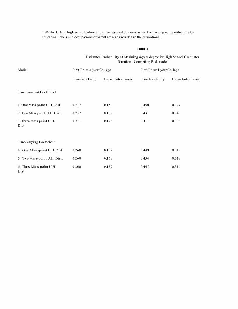
To check the robustness of our estimated impact of delayed entry, Table 4

presents the estimated impact of delaying college enrollment by one year for several

alternative model specifications. Rows 1 through 3 of Table 4 present the estimated

13The model was estimated twice. In the first estimation, those who first enter four-year institutions arecensored in the enrollment duration and in the second estimation, those who first enter two-yearinstitutions are censored in the enrollment duration. In small samples, the two sets of estimates obtainedfor the coefficients in (1') are not necessarily equal. For our data, the two sets of coefficients estimates for(1') do not qualitatively differ. Thus, Tables 4 and 5 present the coefficient estimates for (1') only in thecase where those who enter two-year institutions are censored in the enrollment duration.

21

impacts based on the DCR model with time-constant coefficients when the unobserved

heterogeneity distribution has one, two and three mass points, respectively. Rows 4

through 6 present the estimated impacts based on the DCR model when the coefficient of

the duration until enrollment variable is allowed to vary over time according to a third-

order polynomial and the unobserved heterogeneity distribution has one, two and three

mass points, respectively. Comparing the one mass point estimates to the two and three

mass point estimates indicates that the estimated impact of delay does not change

substantially when the potential endogeneity of delay is accounted for. Comparing rows 1

through 3 with rows 4 through 6 shows that the estimated impacts of enrollment delay

are somewhat larger in models that allow the coefficient of the duration until enrollment

variable to be time-varying.

To account for potential selectivity into two-year versus four-year institutions

due to the unobserved determinants of the two-year, four-year choice being correlated

with the unobservable determinants of completing a four-year degree, Tables 5 reports

estimates derived from the CR2 model described by equations (1') and (2) above.13 The

model estimates in Table 5 are based on the CR2 model where the coefficients of all

22

predictor variables are restricted to be time-constant and the unobserved heterogeneity

distribution is assumed to be characterized by two mass points.

As can be seen in Table 5 an increase in the delay between high school graduation

and college enrollment significantly raises the dropout hazard for both those first entering

two-year institutions and those first entering four-year institutions. The impact of an

increase in enrollment delay on the graduation hazard, while negative both for individuals

first entering two-year and for individuals first entering four-year institutions is

statistically significant only for those first entering two-year institutions.

To assess the magnitude of the effect of delaying enrollment on the probability of

four-year college completion both for those who first enter a two-year institution and for

those who first enter a four-year institution, simulations were performed in which an

individual’s enrollment delay was alternatively set to 0 (enrollment immediately after high

school) and 1 (enrollment after delaying one year ). The college dropout and completion

hazards from these simulations are presented in Figures 6 and 7, respectively, for those

who first enter a four-year institution and Figures 8 and 9, respectively, for those who

first enter a two-year institution. From these hazard estimates, one can show that the

estimated probability of obtaining a four-year degree when the delay until college

enrollment increases from 0 to 1 year declines by 27.7 percent and 25.4 percent for those

first entering four-year and two-year institutions, respectively.

14The estimated impact of four-year tuition levels on attaining a four-year degree for those first enteringtwo-year institutions did not change when a control for two-year in-state public tuition levels was includedin the estimations. Thus, the estimated impact of four-year in-state tuition levels is not due to itscorrelation with two-year in-state tuition levels.

23

To check the robustness of our estimated impact of delayed entry, Table 6

presents the estimated impact of delaying college entry by one year for several alternative

model specifications. The estimated impacts of delaying enrollment by one year on

graduating from a four-year college range from 14.1 to 40.0 percent for individuals first

entering two-year institutions and 11.3 to 32.7 percent for individuals first entering four-

year institutions with the largest estimated impacts coming from those models which

ignore any possible endogeneity of delay.

One result for the other predictor variables that was not evident in the DCR model

estimates has to do with the impact of in-state public tuition levels on four-year college

completion rates. The results from Table 5 show that an increase in public tuition levels

for four-year institutions significantly increases the four-year college dropout rate, but

only among high school graduates who enter two-year institutions. Thus, it appears that

in states with high four-year public tuition levels, individuals who enter two-year

institutions are less likely to transfer to four-year institutions after completing their two-

year degree.14

15Other possible moderators of the impact of delay that were investigated were family income and genderbut only the AFQT score- delay duration interaction achieved statistical significance.

24

Finally, there is some empirical evidence that AFQT scores moderate the impact

of enrollment delay on college graduation.15 Table 7 presents estimates of the impact of

delaying college enrollment by one year for individuals in different AFQT percentile score

categories when AFQT score - duration of enrollment delay interaction variable is

included in the DCR model. As can be seen from the table, the adverse impact of

enrollment delay on the probability of graduation from four-year college is concentrated

primarily among those in the lower AFQT score categories. For example, among those

first entering a four-year institution, the estimated decline in the probability of attaining a

four-year degree by delaying enrollment by one year is 7.6 percent for those with AFQT

percentile scores in the 75-99 range. The estimated decline in the probability of attaining

a four-year degree by delaying enrollment one year increases to 32.9 percent for those

with AFQT percentile scores in the 25-49 range and 52.5 percent for those with AFQT

percentile scores in the 0-24 range.

6. Summary and Concluding Remarks

The main findings of the paper are: First, the delay between high school

graduation and college enrollment is an important determinant of college graduation . The

25

longer a young person takes to enroll in college, the higher the chance is that they do not

graduate.

Second, higher ability individuals, as measured by AFQT scores, are more likely

to enter college, and, among those entering, more likely to finish . Moreover, delaying

enrollment is less costly in terms of reducing the probability of graduating college, for

those with higher AFQT scores.

Third, family background, measured by white-collar occupation and education

levels of parents, family income, and the number of sibling affect college-going behavior. It

is hypothesized that these variables capture the financial resources available to family

and, at the same time, the effect of parents on youths’ aspirations and the degree of

family encouragement.

Fourth, nonwhite high school graduates were found to be more likely than whites

to enter college. Specifically, the competing risks estimates suggest that nonwhites are

more likely to first enter four-year institutions than are whites.

Fifth, an increase in tuition levels for public four-year institutions appears to

reduce the chances that an individual first entering a two-year institution will transfer to a

four-year institution and obtain a four-year degree. There was no evidence that family

income moderated this impact. Also, tuition levels did not appear to affect the college

entry decision or graduation rates of those first entering four-year institutions.

16 Despite this limitation, Dynarski (1999) was able to use the NLSY to examine the impact of financial aidon college attendance. She constructed a variable for whether or not a respondents father died before theywere 18 years of age. She used this variable to proxy for eligibility for Social Security Student Benefitsand found that eligibility for the program raised the probability of attendance by about twenty percentagepoints and that a $1,000 increase in aid increased the probability of attendance by four percentage points.

26

Finally, higher unemployment rates appears to reduce the probability of entering a

four-year institution, increase the risk of dropout and decrease the rate of college

graduation. These results are consistent with the notion that the unemployment rate

reflects financial constraints on college-going behavior.

There are some limitations of the study. First, the NLSY79 does not include

detailed information on financial aid which has been found to affect college behavior

(Cabera, 1992; Edlin, 1993; Fischer, 1992; McPherson and Schapiro2 1998; DesJardins,

Ahlburg and McCall, 2002).16 Second, measures of employment opportunities rather than

the unemployment rate have not been investigated. Third, information on the

characteristics of the colleges considered or attended and the GPA attained by individuals

while at a particular institution were not available. This latter information may give one

indication of the student-institution match. Finally, a limitation of this study was that

only one year of average in-state tuition data was used to measure the tuition costs facing

an individual. More detailed data on public and private, two-year and four-year

institution tuition may give better estimates of the impact of relative tuition rates on

college choice and post-secondary educational attainment.

27

One policy implication suggested by the findings of this paper is that high school

guidance counselors may wish to caution students against delaying college enrollment,

especially students with low test scores. Such a delay may lead to lower post-secondary

educational attainment and, in turn, lower future earnings for these students. Colleges may

also wish to develop and target programs towards delayed enrollees that will increase

their chances of completion.

28

Appendix

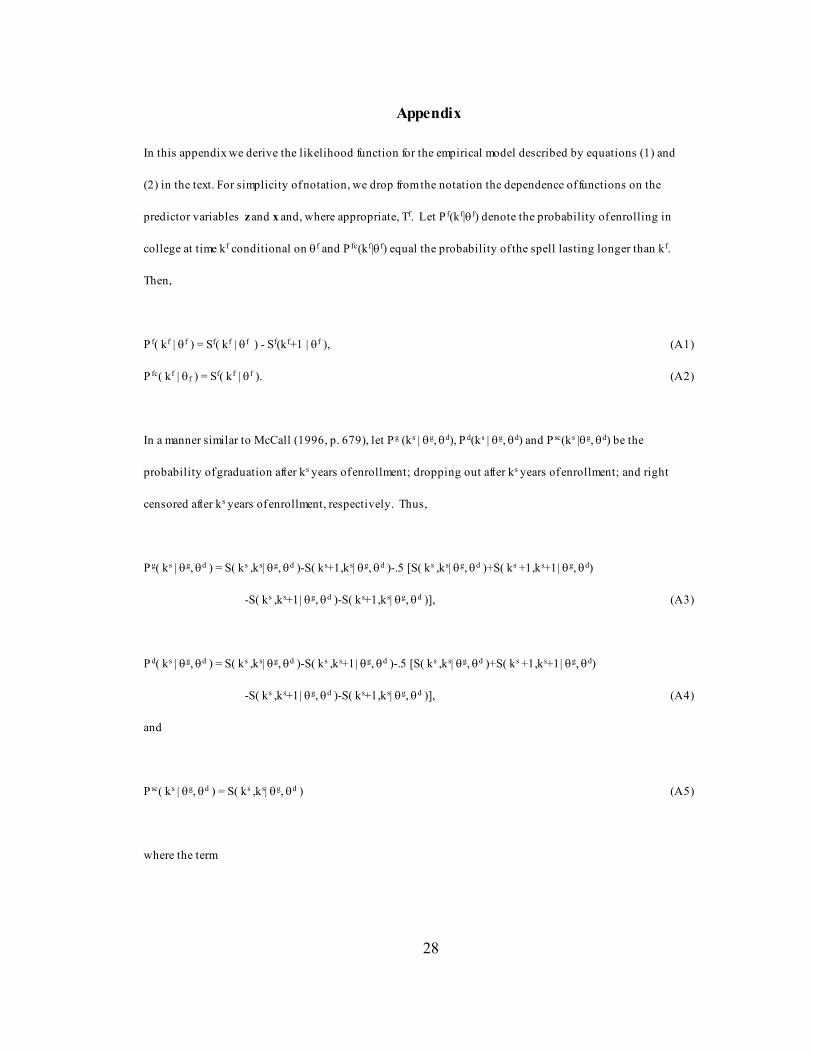
In this appendix we derive the likelihood function for the empirical model described by equations (1) and

(2) in the text. For simplicity of notation, we drop from the notation the dependence of functions on the

predictor variables z and x and, where appropriate, Tf. Let P f(kf|θf) denote the probability of enrolling in

college at time kf conditional on θf and P fc(kf|θf) equal the probability of the spell lasting longer than kf.

Then,

P f( kf | θf ) = Sf( kf | θf ) - Sf(kf+1 | θf ), (A1)

P fc( kf | θf ) = Sf( kf | θf ). (A2)

In a manner similar to McCall (1996, p. 679), let Pg (ks | θg, θd), P d(ks | θg, θd) and P sc(ks |θg, θd) be the

probability of graduation after ks years of enrollment; dropping out after ks years of enrollment; and right

censored after ks years of enrollment, respectively. Thus,

P g( ks | θg, θd ) = S( ks ,ks| θg, θd )-S( ks+1,ks| θg, θd )-.5 [S( ks ,ks| θg, θd )+S( ks +1,ks+1| θg, θd)

-S( ks ,ks+1| θg, θd )-S( ks+1,ks| θg, θd )], (A3)

P d( ks | θg, θd ) = S( ks ,ks| θg, θd )-S( ks ,ks+1| θg, θd )-.5 [S( ks ,ks| θg, θd )+S( ks +1,ks+1| θg, θd)

-S( ks ,ks+1| θg, θd )-S( ks+1,ks| θg, θd )], (A4)

and

P sc( ks | θg, θd ) = S( ks ,ks| θg, θd ) (A5)

where the term

29

log log( ( , ))L q B k kiw w

if

is

w Wi

M

=∈=∑∑

1

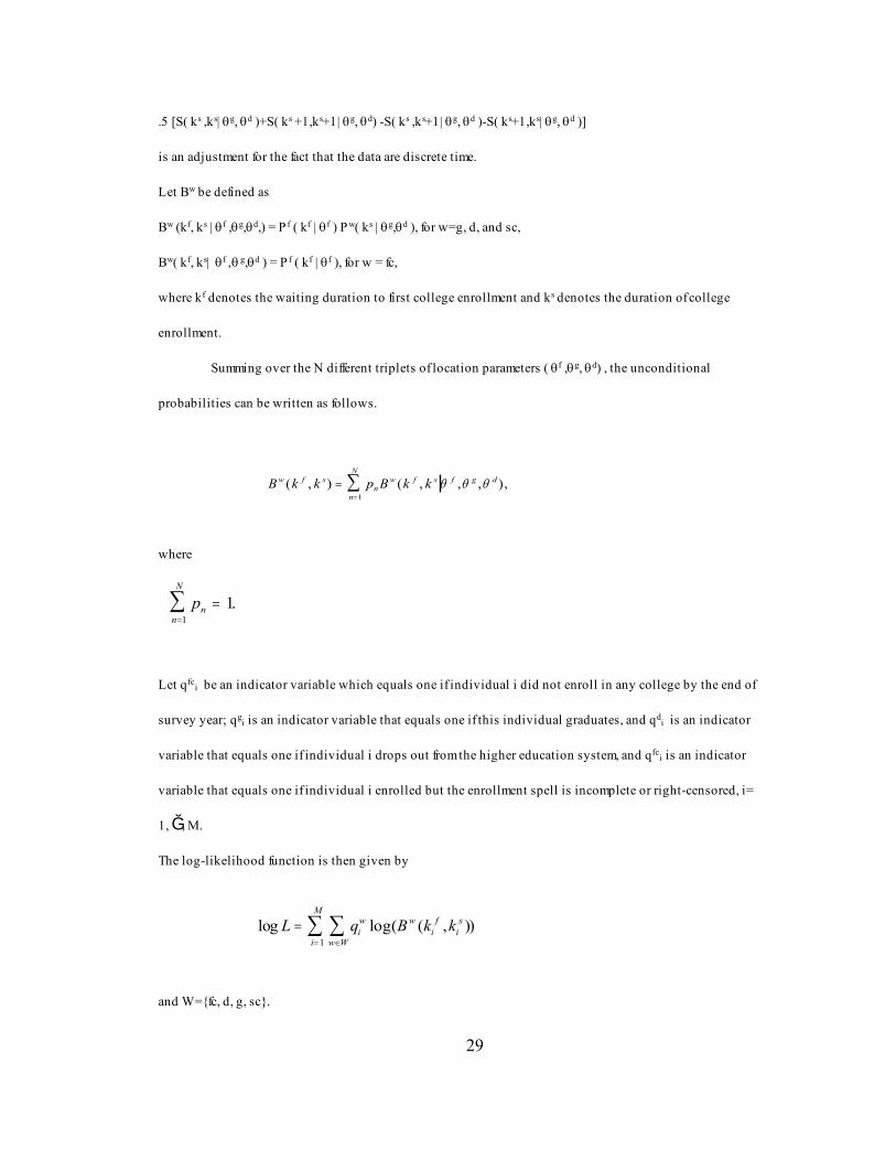
.5 [S( ks ,ks| θg, θd )+S( ks +1,ks+1| θg, θd) -S( ks ,ks+1| θg, θd )-S( ks+1,ks| θg, θd )]

is an adjustment for the fact that the data are discrete time.

Let Bw be defined as

Bw (kf, ks | θf ,θg,θd,) = P f ( kf | θf ) P w( ks | θg,θd ), for w=g, d, and sc,

Bw( kf, ks| θf ,θ g,θd ) = P f ( kf | θf ), for w = fc,

where kf denotes the waiting duration to first college enrollment and ks denotes the duration of college

enrollment.

Summing over the N different triplets of location parameters ( θf ,θg, θd) , the unconditional

probabilities can be written as follows.

B k k p B k kw f sn

w f s f g d

n

N

( , ) ( , , , ),==∑ θ θ θ

1

where

pnn

N

=∑ =

11.

Let qfci be an indicator variable which equals one if individual i did not enroll in any college by the end of

survey year; qgi is an indicator variable that equals one if this individual graduates, and qd

i is an indicator

variable that equals one if individual i drops out from the higher education system, and qfci is an indicator

variable that equals one if individual i enrolled but the enrollment spell is incomplete or right-censored, i=

1, þ, M.

The log-likelihood function is then given by

and W={fc, d, g, sc}.

30

References

Adelman, Clifford. (1999), Answers in the Tool Box: Academic Intensity, AttendancePatterns, and Bachelor’s Degree Attainment. Jessup, MD: U.S. Department ofEducation.

Altonji, Joseph G. (1993), “The Demand for and Return to Education when EducationOutcomes are Uncertain,” Journal of Labor Economics, 11, 48-83.

Anderson, Patricia M. (1992), “Time-varying Effects of Recall Expectation, aReemployment Bonus, and Job Counseling on Unemployment Durations,”Journal of Labor Economics, 10-1, 99-115.

Blakemore, Arthur and Stuart Low (1984), "The High School Dropout Decision and ItsWage Consequences,” Economics of Education Review, 3-2, 111-119.

Blanchfield, William (1972), "College Dropout Identification: An Economic Analysis,”Journal of Human Resources, 7-4, 540-544.

Bound, John and George Johnson (1989), “Changes in the Structure of Wages During the1980s: An Evaluation of Alternative Explanations,” Working Paper no. 2983,NBER.

Brewer, Dominic J., Eric R. Eide, and Ronald G. Ehrenberg (1999), “Does it Pay toAttend an Elite Private College?” Journal of Human Resources, 24: 105-123.

Cabera, A.F. et al. (1992), “The Role of Finances in the Persistence Process: A StructureModel,” Research in Higher Education, 33-5, 571-593.

Cameron, Stephen V. and James J. Heckman (1993), “The Nonequivalence of High SchoolEquivalents” Journal of Labor Economics, 11, 1-47.

Cameron, Stephen V. and James J. Heckman (1998), “Life Cycle Schooling and DynamicSelection Bias: Models and Evidence for Five Cohorts of American Males,”Journal of Political Economy, 106, 263-333.

31

Cameron, Stephen V. and James J. Heckman (2000), “The Dynamics of EducationalAttainment for Black, Hispanic, and White Males,” mimeo, University ofChicago.

DesJardins, Stephan L; Dennis A. Ahlburg and Brian P. McCall (2002), “Simulating theLongitudinal Effects of Changes in Financial Aid on Student Departure fromCollege,” Journal of Human Resources, 37-3.

Diaz-Jiminez, J., V. Quadrini, and J-V Rios-Rull (1997), “Dimensions of Inequality:Facts on the U.S. Distribution of Earnings, Income and Wealth,” Federal ReserveBank of Minneapolis Quarterly Review Spring: 3-21.

Dynarski, Susan .M. (1999), “Does Aid Matter? Measuring the Effect of Student Aid onCollege Attendance and Completion,” Working Paper no. 7422. NBER.

Eagle, Eva and C. Dennis Carroll (1988), Postsecondary Enrollment, Persistence, andAttainment for 1972, 1980, and 1982 High School Graduates” US Department ofEducation, National Center for Educational Statistics, Office of Research andImprovement. Survey Report High School and Beyond National LongitudinalStudy Data Series DR-NLS/HSB: 72-86.

Edlin, Aaron (1993), "Is College Financial Aid Equitable and Efficient?,” Journal ofEconomic Perspectives, 7-2, 143-158.

Fischer, F. (1992), “Graduation-Contingent Aid,” Change, 40-47.

Han, Aaron and Jerry Hausman (1990), “Flexible Parametric Estimation of Duration andCompeting Risks Models,” Journal of Applied Econometrics, 5-1, 1-28.

Kane, John (1994), “College Entry by Blacks since 1970: The Role of College Costs,Family Background, and the Returns to Education,” Journal of Political Economy,102-5, 878-911.

Kane, John and Cecilia E. Rouse (1995), “Labor-Market Returns to Two- and Four-yearCollege,” American Economic Review, 85-3, 600-614.

32

Kane, John and Lawrence M. Spizman (1994), “Race, Financial Aid Awards and CollegeAttendance: Parents and Geography Matter,” American Journal of Economics andSociology, 53-1, 85-97.

Katz, Lawrence F. (1986), “Layoffs, Recalls and the Duration of Unemployment,”NBER Working Paper No. 1825.

Kiefer, Nicholas (1988), “Economic Duration Data and Hazard Function,” Journal ofEconomic Literature, 26, 646-679.

Kominski, Robert (1990), “Estimating the National High School Dropout Rate,”Demography, 27-2, 303-311.

Light, Audrey (1995a), “The Effect of Interrupted Schooling on Wages,” The Journal ofHuman Resources, 30-3, 473-502.

Light, Audrey (1995b), “Hazard Model Estimates of the Decision to Reenroll in School,”Labour Economics, 2, 381-406.

McCall, Brian P. (1990), “Occupational Matching: A Test of Sorts,” Journal of PoliticalEconomy, 98, 45-69.

McCall, Brian P. (1996), “Unemployment Insurance Rules, Joblessness, and Part-TimeWork,” Econometrica, 64-3, 647-682.

McLanahan, Sara (1985), “Family Structure and the Reproduction of Poverty,” AmericanJournal of Sociology, 90-4, 873-901.

McPherson, Michael S. and Morton O. Schapiro. (1998) The Student Aid Game(Princeton, NJ: Princeton University Press).

Manski, Charles F. (1989), “Schooling as Experimentation: A Reappraisal of thePostsecondary Dropout Phenomenon,” Economics of Education Review, 8-4, 305-312.

Manski, Charles F. and David Wise (1983), College Choice in America, ( Mass.:HarvardUniversity Press)

33

Meyer, Bruce D. (1990), “Unemployment Insurance and Unemployment Spells,”Econometrica, 58-4, 757-782.

Miller, Robert A. (1984), “Job Matching and Occupational Choice,” Journal of PoliticalEconomy, 92, 1086-1120.

Murphy, Kevin and Finis Welch (1993), Inequality and Relative Wages,” AmericanEconomic Review, (83,2) May: 104-109.

National Center for Education Statistics (2001), "Educational Achievement and Black-White Inequality,” Statistical Analysis Report NCES 2001-061.

National Center for Education Statistics (1989), "College Persistence and DegreeAttainment for 1980 High School Graduates: Hazards for Transfers, Stopouts,and Part-timers," Survey Report, CS89-302.

34

Narendranathan, S.W. and M. B. Stewart (1990), “An Examination of the Robustness ofModels of the Probability of Finding a Job for the Unemployed,” in J. Hartog, G.Ridder and J. Theuwes (eds.), Panel Data and Labor Market Studies, (New York:North-Holland), 135-155.

Neal, Derek (1999), “The Complexity of Job Mobility among Young Men,” Journal ofLabor Economics, 17, 237-261.

Sueyoshi, Glenn (1992), “Semiparametric Proportional Hazards Estimation of CompetingRisks Models with Time-Varying Covariates,” Journal of Econometrics, 51, 25-58.

Tinto, Vincent (1988), “Stages of Student Departure: Reflections on the LongitudinalCharacter of Student Leaving,” Journal of Higher Education, 59-4, 483-455.

Tinto, Vincent (1993), Leaving College, (Chicago: University of Chicago Press).

U.S. Department of Education, Digest of Education Statistics, various issues.

U.S. Department of Education, (1989), College Persistence and Degree Attainment for1980 High school Graduates: Hazards for Transfers, Stopouts, and Part-timers,US Department of Education, National Center for Educational Statistics, Office ofEducational Research and Improvement. Survey Report. Data Series 80/86.

Willis, Robert J. and Sherwin Rosen (1979), “Education and Self-Selection,” Journal ofPolitical Economy, 87, S7-S36.

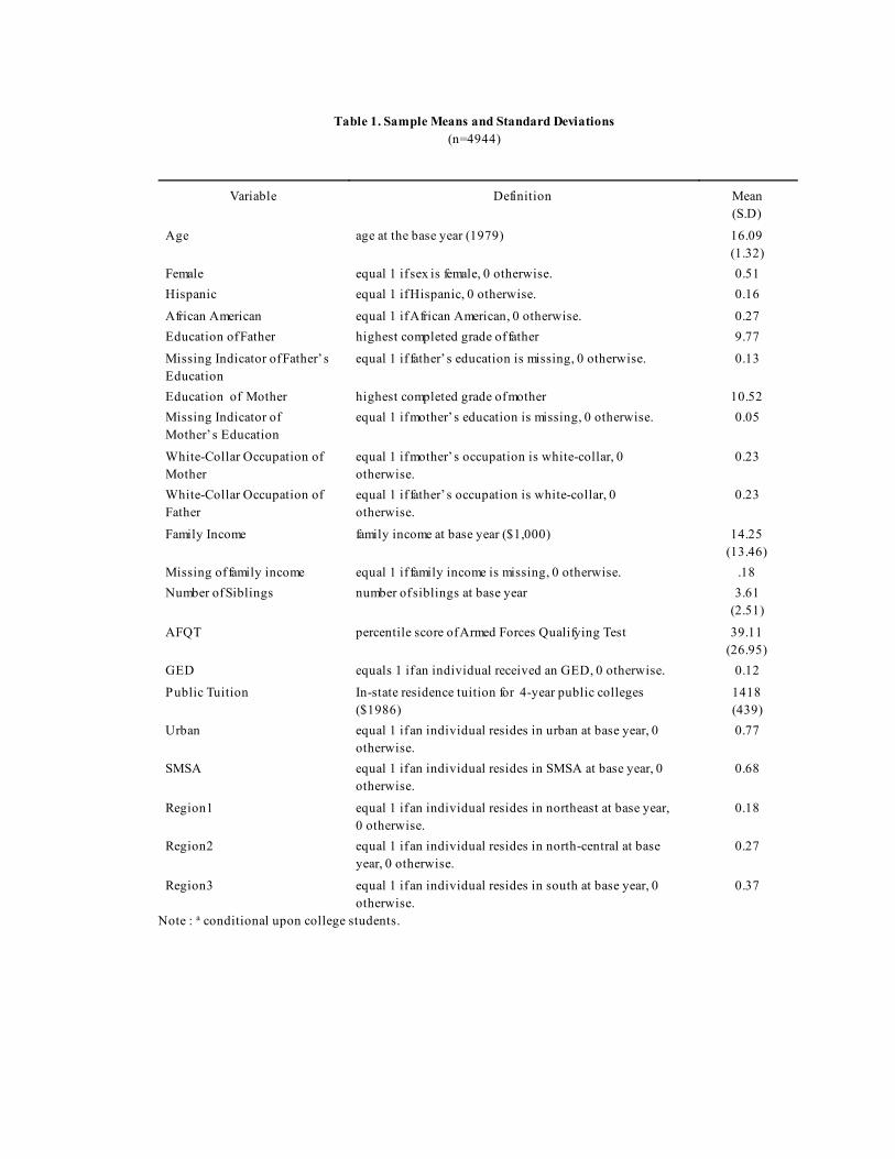
Table 1. Sample Means and Standard Deviations(n=4944)

Variable Definition Mean(S.D)

Age age at the base year (1979) 16.09(1.32)

Female equal 1 if sex is female, 0 otherwise. 0.51Hispanic equal 1 if Hispanic, 0 otherwise. 0.16

African American equal 1 if African American, 0 otherwise. 0.27Education of Father highest completed grade of father 9.77

Missing Indicator of Father’sEducation

equal 1 if father’s education is missing, 0 otherwise. 0.13

Education of Mother highest completed grade of mother 10.52Missing Indicator ofMother’s Education

equal 1 if mother’s education is missing, 0 otherwise. 0.05

White-Collar Occupation of Mother

equal 1 if mother’s occupation is white-collar, 0otherwise.

0.23

White-Collar Occupation of Father

equal 1 if father’s occupation is white-collar, 0otherwise.

0.23

Family Income family income at base year ($1,000) 14.25(13.46)

Missing of family income equal 1 if family income is missing, 0 otherwise. .18Number of Siblings number of siblings at base year 3.61

(2.51)

AFQT percentile score of Armed Forces Qualifying Test 39.11(26.95)

GED equals 1 if an individual received an GED, 0 otherwise. 0.12

Public Tuition In-state residence tuition for 4-year public colleges($1986)

1418(439)

Urban equal 1 if an individual resides in urban at base year, 0otherwise.

0.77

SMSA equal 1 if an individual resides in SMSA at base year, 0otherwise.

0.68

Region1 equal 1 if an individual resides in northeast at base year,0 otherwise.

0.18

Region2 equal 1 if an individual resides in north-central at baseyear, 0 otherwise.

0.27

Region3 equal 1 if an individual resides in south at base year, 0otherwise.

0.37

Note : a conditional upon college students.

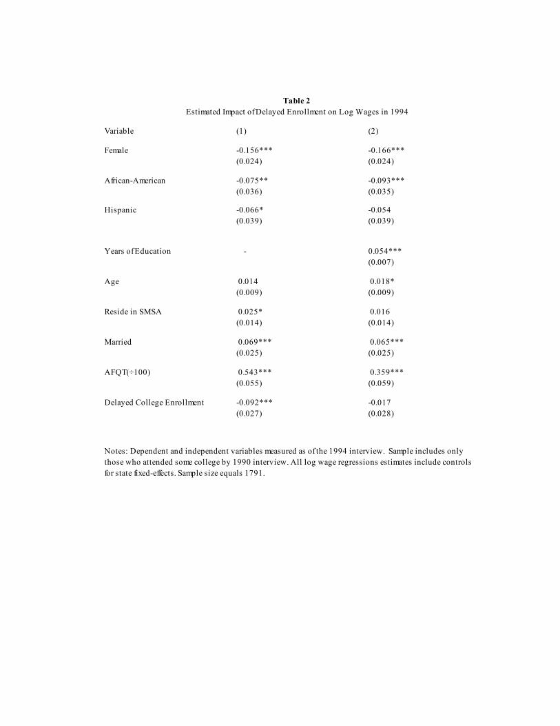
Table 2Estimated Impact of Delayed Enrollment on Log Wages in 1994

Variable (1) (2)

Female -0.156***(0.024)

-0.166***(0.024)

African-American -0.075**(0.036)

-0.093***(0.035)

Hispanic -0.066*(0.039)

-0.054(0.039)

Years of Education - 0.054***(0.007)

Age 0.014(0.009)

0.018*(0.009)

Reside in SMSA 0.025*(0.014)

0.016(0.014)

Married 0.069***(0.025)

0.065***(0.025)

AFQT(÷100) 0.543***(0.055)

0.359***(0.059)

Delayed College Enrollment -0.092***(0.027)

-0.017(0.028)

Notes: Dependent and independent variables measured as of the 1994 interview. Sample includes onlythose who attended some college by 1990 interview. All log wage regressions estimates include controlsfor state fixed-effects. Sample size equals 1791.

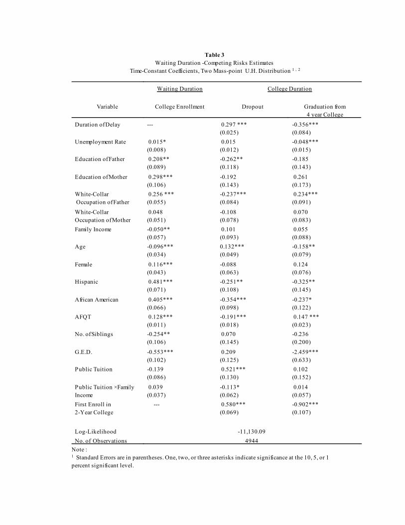
Table 3Waiting Duration -Competing Risks Estimates

Time-Constant Coefficients, Two Mass-point U.H. Distribution 1 , 2

Waiting Duration College Duration

Variable College Enrollment Dropout Graduation from4 year College

Duration of Delay --- 0.297 ***(0.025)

-0.356***(0.084)

Unemployment Rate 0.015*(0.008)

0.015(0.012)

-0.048*** (0.015)

Education of Father 0.208**(0.089)

-0.262** (0.118)

-0.185(0.143)

Education of Mother 0.298***(0.106)

-0.192(0.143)

0.261(0.173)

White-Collar Occupation of Father

0.256 ***(0.055)

-0.237***(0.084)

0.234***(0.091)

White-CollarOccupation of Mother

0.048(0.051)

-0.108(0.078)

0.070 (0.083)

Family Income -0.050**(0.057)

0.101(0.093)

0.055(0.088)

Age -0.096***(0.034)

0.132***(0.049)

-0.158**(0.079)

Female 0.116***(0.043)

-0.088(0.063)

0.124(0.076)

Hispanic 0.481***(0.071)

-0.251**(0.108)

-0.325** (0.145)

African American 0.405***(0.066)

-0.354***(0.098)

-0.237*(0.122)

AFQT 0.128***(0.011)

-0.191***(0.018)

0.147 ***(0.023)

No. of Siblings -0.254**(0.106)

0.070(0.145)

-0.236(0.200)

G.E.D. -0.553***(0.102)

0.209(0.125)

-2.459***(0.633)

Public Tuition -0.139(0.086)

0.521***(0.130)

0.102(0.152)

Public Tuition ×FamilyIncome

0.039(0.037)

-0.113*(0.062)

0.014(0.057)

First Enroll in 2-Year College

--- 0.580***(0.069)

-0.902***(0.107)

Log-Likelihood -11,130.09No. of Observations 4944

Note : 1 Standard Errors are in parentheses. One, two, or three asterisks indicate significance at the 10, 5, or 1percent significant level.

2 SMSA, Urban, high school cohort and three regional dummies as well as missing value indicators foreducation levels and occupations of parent are also included in the estimations.

Table 4

Estimated Probability of Attaining 4-year degree for High School GraduatesDuration - Competing Risk model

Model First Enter 2-year College First Enter 4-year College

Immediate Entry Delay Entry 1-year Immediate Entry Delay Entry 1-year

Time Constant Coefficient

1. One Mass point U.H. Dist. 0.217 0.159 0.450 0.327

2. Two Mass point U.H. Dist. 0.237 0.167 0.431 0.340

3. Three Mass point U.H.Dist.

0.231 0.174 0.411 0.334

Time-Varying Coefficient

4. One Mass-point U.H. Dist. 0.260 0.159 0.449 0.313

5. Two Mass-point U.H. Dist. 0.260 0.158 0.454 0.318

6. Three Mass-point U.H.Dist.

0.260 0.159 0.447 0.314

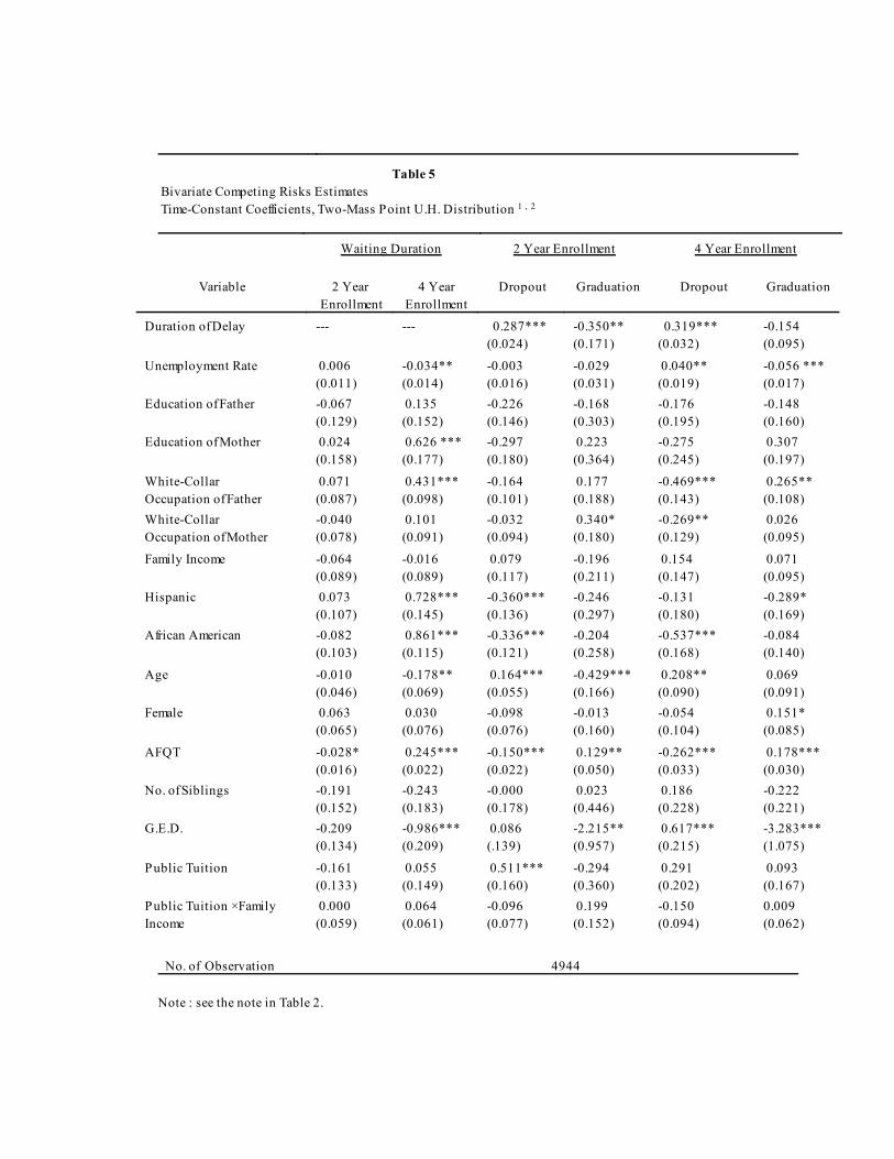
Table 5 Bivariate Competing Risks Estimates Time-Constant Coefficients, Two-Mass Point U.H. Distribution 1 , 2

Waiting Duration 2 Year Enrollment 4 Year Enrollment

Variable 2 Year Enrollment

4 Year Enrollment

Dropout Graduation Dropout Graduation

Duration of Delay --- --- 0.287***(0.024)

-0.350** (0.171)

0.319***(0.032)

-0.154 (0.095)

Unemployment Rate 0.006(0.011)

-0.034**(0.014)

-0.003(0.016)

-0.029(0.031)

0.040**(0.019)

-0.056 ***(0.017)

Education of Father -0.067(0.129)

0.135(0.152)

-0.226(0.146)

-0.168(0.303)

-0.176(0.195)

-0.148(0.160)

Education of Mother 0.024(0.158)

0.626 ***(0.177)

-0.297(0.180)

0.223(0.364)

-0.275(0.245)

0.307(0.197)

White-Collar Occupation of Father

0.071(0.087)

0.431***(0.098)

-0.164(0.101)

0.177(0.188)

-0.469***(0.143)

0.265**(0.108)

White-CollarOccupation of Mother

-0.040(0.078)

0.101(0.091)

-0.032(0.094)

0.340*(0.180)

-0.269**(0.129)

0.026(0.095)

Family Income -0.064(0.089)

-0.016(0.089)

0.079(0.117)

-0.196(0.211)

0.154(0.147)

0.071(0.095)

Hispanic 0.073(0.107)

0.728***(0.145)

-0.360***(0.136)

-0.246(0.297)

-0.131(0.180)

-0.289*(0.169)

African American -0.082(0.103)

0.861***(0.115)

-0.336***(0.121)

-0.204 (0.258)

-0.537***(0.168)

-0.084 (0.140)

Age -0.010(0.046)

-0.178**(0.069)

0.164***(0.055)

-0.429***(0.166)

0.208**(0.090)

0.069(0.091)

Female 0.063(0.065)

0.030(0.076)

-0.098(0.076)

-0.013(0.160)

-0.054(0.104)

0.151*(0.085)

AFQT -0.028*(0.016)

0.245***(0.022)

-0.150***(0.022)

0.129**(0.050)

-0.262***(0.033)

0.178***(0.030)

No. of Siblings -0.191(0.152)

-0.243(0.183)

-0.000(0.178)

0.023(0.446)

0.186(0.228)

-0.222(0.221)

G.E.D. -0.209(0.134)

-0.986***(0.209)

0.086(.139)

-2.215**(0.957)

0.617***(0.215)

-3.283***(1.075)

Public Tuition -0.161(0.133)

0.055(0.149)

0.511***(0.160)

-0.294(0.360)

0.291(0.202)

0.093(0.167)

Public Tuition ×FamilyIncome

0.000(0.059)

0.064(0.061)

-0.096(0.077)

0.199(0.152)

-0.150(0.094)

0.009(0.062)

No. of Observation 4944

Note : see the note in Table 2.

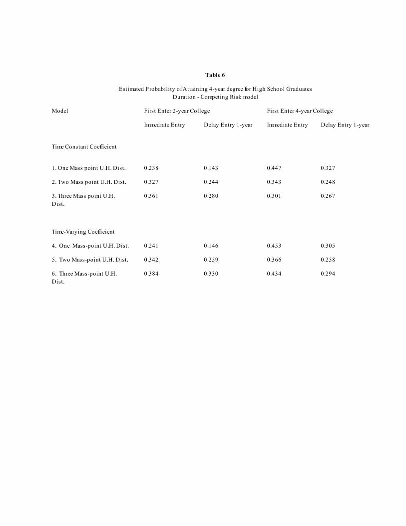
Table 6

Estimated Probability of Attaining 4-year degree for High School GraduatesDuration - Competing Risk model

Model First Enter 2-year College First Enter 4-year College

Immediate Entry Delay Entry 1-year Immediate Entry Delay Entry 1-year

Time Constant Coefficient

1. One Mass point U.H. Dist. 0.238 0.143 0.447 0.327

2. Two Mass point U.H. Dist. 0.327 0.244 0.343 0.248

3. Three Mass point U.H.Dist.

0.361 0.280 0.301 0.267

Time-Varying Coefficient

4. One Mass-point U.H. Dist. 0.241 0.146 0.453 0.305

5. Two Mass-point U.H. Dist. 0.342 0.259 0.366 0.258

6. Three Mass-point U.H.Dist.

0.384 0.330 0.434 0.294

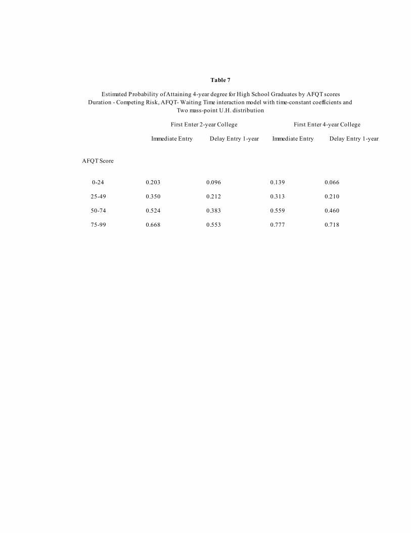
Table 7

Estimated Probability of Attaining 4-year degree for High School Graduates by AFQT scoresDuration - Competing Risk, AFQT- Waiting Time interaction model with time-constant coefficients and

Two mass-point U.H. distribution

First Enter 2-year College First Enter 4-year College

Immediate Entry Delay Entry 1-year Immediate Entry Delay Entry 1-year

AFQT Score

0-24 0.203 0.096 0.139 0.066

25-49 0.350 0.212 0.313 0.210

50-74 0.524 0.383 0.559 0.460

75-99 0.668 0.553 0.777 0.718

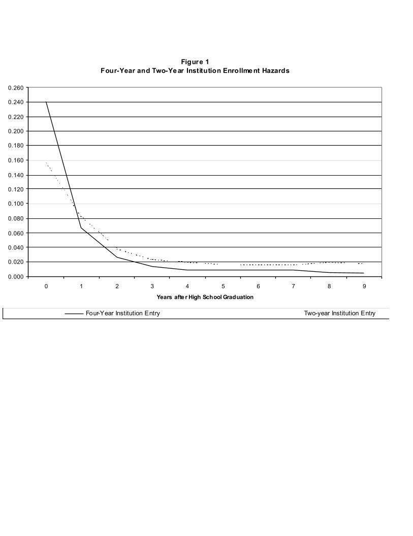
Figure 1Four-Year and Two-Year Institution Enrollment Hazards

0.000

0.020

0.040

0.060

0.080

0.100

0.120

0.140

0.160

0.180

0.200

0.220

0.240

0.260

0 1 2 3 4 5 6 7 8 9

Years afte r High School Graduation

Four-Year Institution Entry Two-year Institution Entry

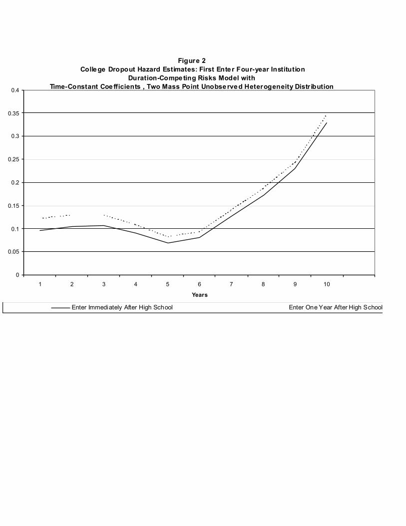
Figure 2 College Dropout Hazard Estimates: First Ente r Four-year Institution

Duration-Competing Risks Model withTime-Constant Coe fficients , Two Mass Point Unobserved Heterogeneity Distr ibution

0

0.05

0.1

0.15

0.2

0.25

0.3

0.35

0.4

1 2 3 4 5 6 7 8 9 10

Years

Enter Immediately After High School Enter One Year After High School

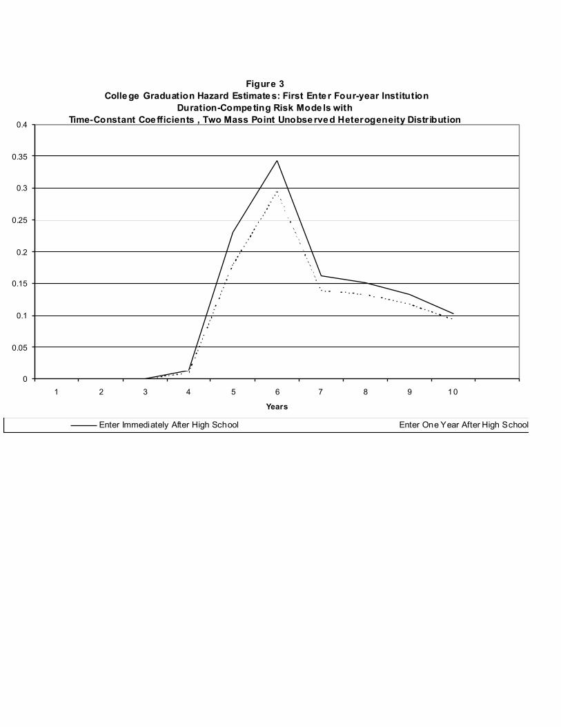
Figure 3 College Graduation Hazard Estimates: First Ente r Four-year Institution

Duration-Competing Risk Mode ls withTime-Constant Coe fficients , Two Mass Point Unobserved Heterogeneity Distr ibution

0

0.05

0.1

0.15

0.2

0.25

0.3

0.35

0.4

1 2 3 4 5 6 7 8 9 10

Years

Enter Immediately After High School Enter One Year After High School

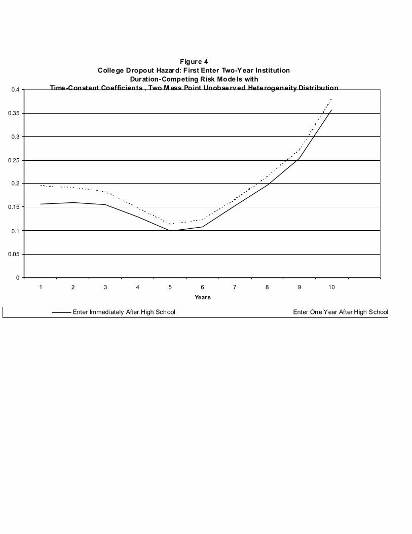
Figure 4College Dropout Hazard: First Enter Two-Year Institution

Duration-Competing Risk Mode ls withTime-Constant Coefficients , Two M ass Point Unobserved Hete rogeneity Distr ibution

0

0.05

0.1

0.15

0.2

0.25

0.3

0.35

0.4

1 2 3 4 5 6 7 8 9 10

Years

Enter Immediately After High School Enter One Year After High School

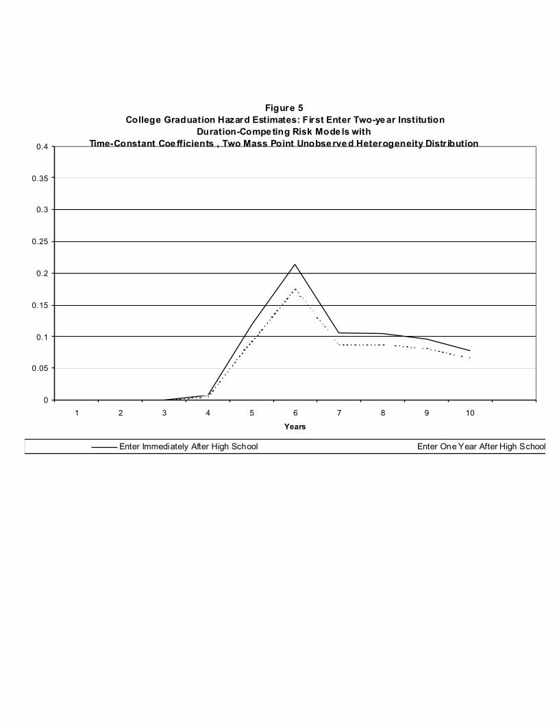
Figure 5 College Graduation Hazard Estimates: First Enter Two-year Institution

Duration-Competing Risk Mode ls withTime-Constant Coe fficients , Two Mass Point Unobserved Heterogeneity Distr ibution

0

0.05

0.1

0.15

0.2

0.25

0.3

0.35

0.4

1 2 3 4 5 6 7 8 9 10

Years

Enter Immediately After High School Enter One Year After High School

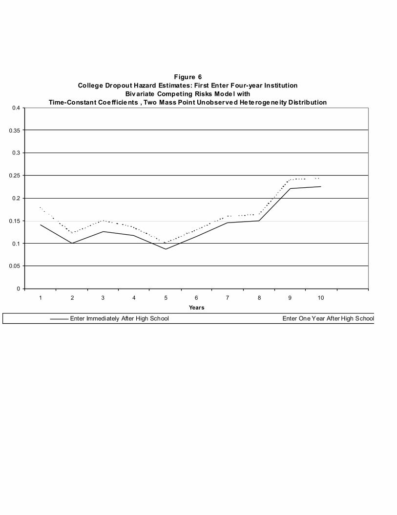
Figure 6College Dropout Hazard Estimates: First Enter Four-year Institution

Bivariate Competing Risks Mode l withTime-Constant Coe fficients , Two Mass Point Unobserved He te rogene ity Distribution

0

0.05

0.1

0.15

0.2

0.25

0.3

0.35

0.4

1 2 3 4 5 6 7 8 9 10

Years

Enter Immediately After High School Enter One Year After High School

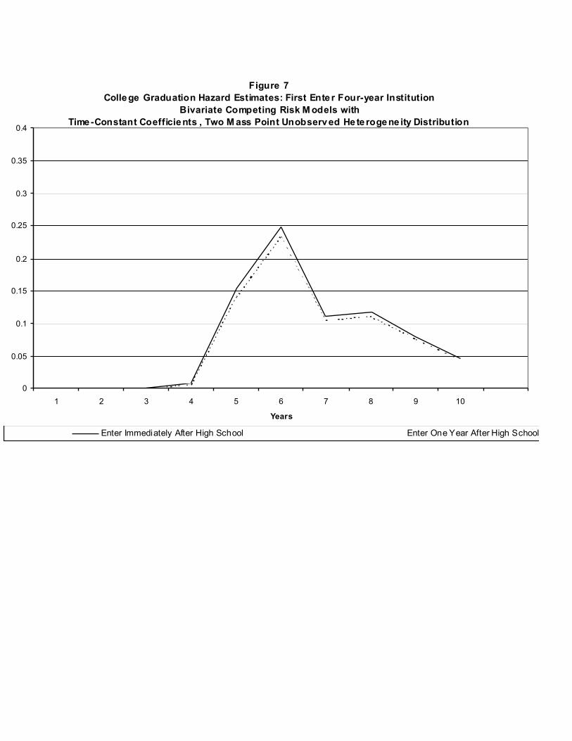
Figure 7College Graduation Hazard Estimates: First Ente r Four-year Institution

Bivariate Competing Risk M odels withTime-Constant Coefficients , Two M ass Point Unobserved He te rogene ity Distribution

0

0.05

0.1

0.15

0.2

0.25

0.3

0.35

0.4

1 2 3 4 5 6 7 8 9 10

Years

Enter Immediately After High School Enter One Year After High School

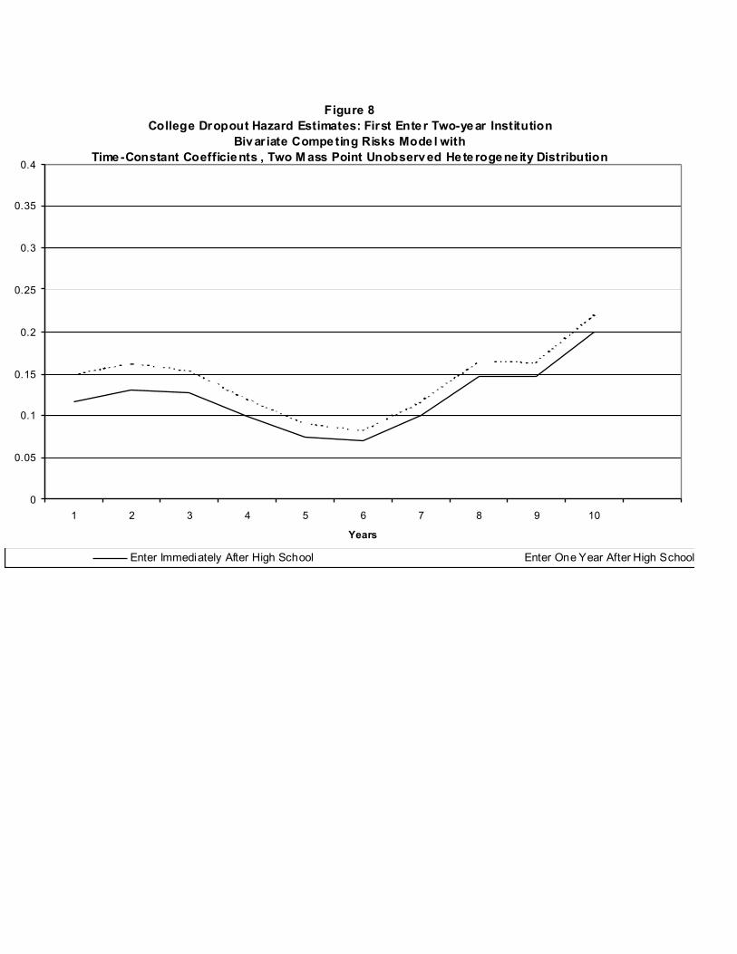
Figure 8College Dropout Hazard Estimates: First Ente r Two-year Institution

Bivariate Competing Risks Mode l withTime-Constant Coefficients , Two M ass Point Unobserved He te rogene ity Distribution

0

0.05

0.1

0.15

0.2

0.25

0.3

0.35

0.4

1 2 3 4 5 6 7 8 9 10

Years

Enter Immediately After High School Enter One Year After High School

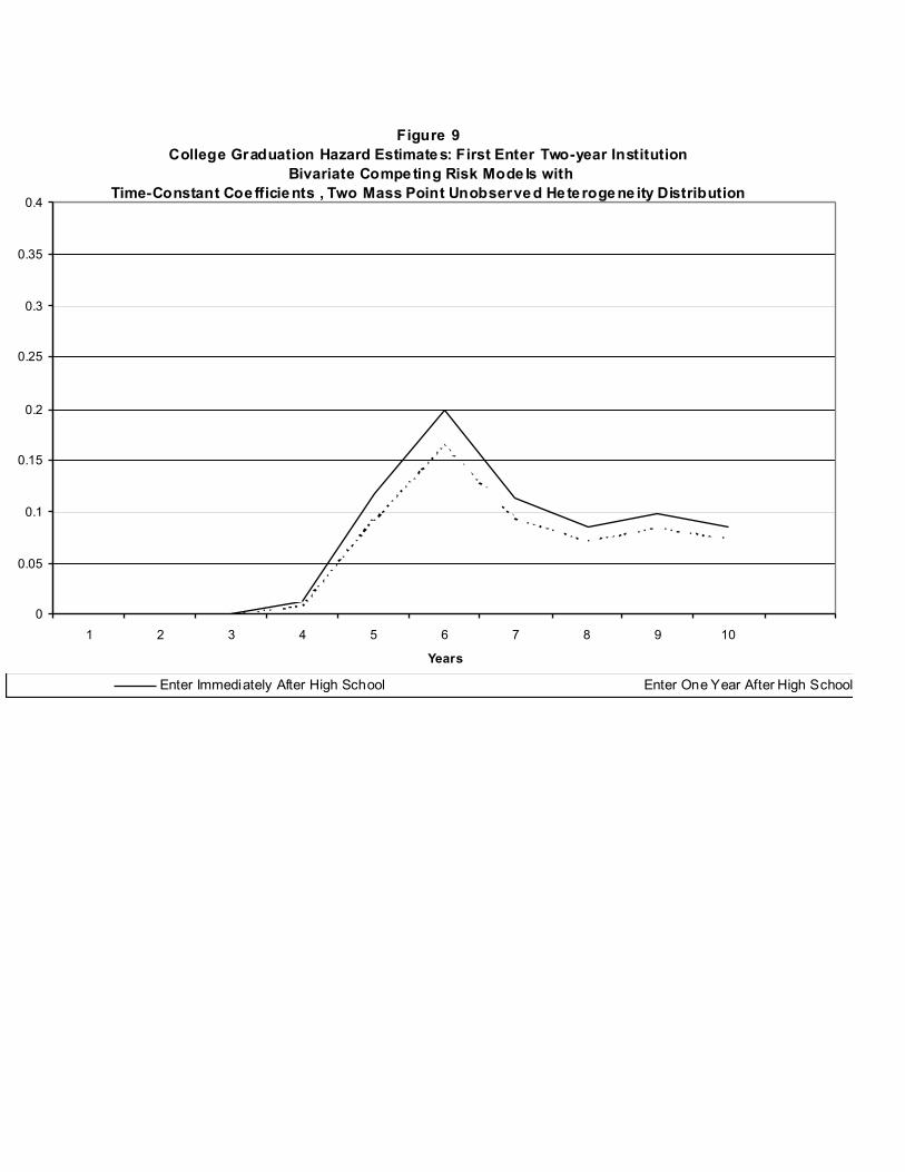
Figure 9College Graduation Hazard Estimates: First Enter Two-year Institution

Bivariate Competing Risk Mode ls withTime-Constant Coe fficients , Two Mass Point Unobserved He te rogene ity Distribution

0

0.05

0.1

0.15

0.2

0.25

0.3

0.35

0.4

1 2 3 4 5 6 7 8 9 10

Years

Enter Immediately After High School Enter One Year After High School