Time-since-infection Immunological Model for Hepatitis C and

Observed Treatment Profiles

Swati DebRoyUniversity of Florida.

Faculty Advisors:Carlos Castillo-Chavez1, Maia Martcheva 2, Anuj Mubayi1,3

1. Arizona State University, 2.University of Florida 3. University of Texas, Arlington,

August 5, 2009

Abstract

Hepatitis C infection becomes chronic in most patients leading to end-stage liver disease. Thestandard-of-care treatment for HCV patients is only suboptimal. Several patients who exhibitundetectable viral load during, at the end of, or six months after cessation of therapy, observesrelapse over variable time. This suggests that there may exist, a sub-clinical threshold, whichgoverns the achievement of lasting cure. We propose an immunological model of hepatocytes andHCV to investigate this threshold behavior, where the infected hepatocytes are differentiatedby the age of infection in them. The goal of the model is to obtain observed patient profilesif treatment is provided. Preliminary analysis of the model provides conditions for existenceof two endemic equilibria for R0 < 1. Analysis of a reduced model without age of infectionsuggests backward bifurcation at R0 = 1. Artificial values of the parameters are taken to showbistability region for R0 < 1. However, it may not be possible to observe the patient profile inthis region without treatment. The critical reproduction number below which the disease freeequilibrium is stable may lead us to the decisive sub-clinical viral load threshold.

Keywords: Interferon, ribavirin, Hepatitis C, HCV,Abbreviations: HCV, Hepatitis C virus, peg-IFN, pegylated Interferon, RBV, Ribavirin,

1

1 Introduction

About one hundred and seventy million people live with Hepatitis C virus (HCV) infection world-wide [?]. Currently, there is no vaccine for HCV. The major mode of transmission of HCV is byexposure to infected blood. Sexual transmission is observed only in people coinfected with HIV andvertical transmission of HCV is rare [?]. The HCV infects hepatocytes which form a major portionof the cytoplasmic mass of the liver. Although HCV predominantly replicates in hepatocytes, tracesof it have been detected in other cell types [?, ?]. Around 15-30% of the acutely infected HepatitisC patients who are asymptomatic and more than 50% of patients with symptoms spontaneouslyclear the virus [?], observed more in infants and young women. Whereas, in 55-75% people whodevelop acute Hepatitis C remain infected [?]. In the the Hep-C patients where the immune systemcannot clear the virus by itself medical intervention is necessary. A combination of drugs, Interferon(IFN-α) and ribavirin (RBV) is prescribed for 24 to 48 weeks [?].

Hepatitis C virus (HCV) is a very slowly evolving disease, where chronic HCV infection cancontinue for decades, with or without treatment. Due to this reason it has not been proved beyonddoubt that treatment provides absolute cure and halts progression to adverse liver infections likecirrhosis and hepatocellular carcinoma among others. Thus therapy of HCV is primarily targetedtowards restricting deterioration of liver condition necessitating liver transplant or causing patient’sdeath.

As a consequence, response in patients to treatment are measured by ”surrogate virologicalparameter”, instead of a specific ”clinical end-point”. Several types of virological response thresh-olds are defined depending on time, relative to treatment duration, having differential degree ofreliability as a prescient of long term clinical cure [?].

The most important among these is the sustained virological response (SVR), which is theabsence of HCV viral load after six months beyond therapy cessation. SVR is largely considered as”virological cure” and usually followed by years of no drastic decline in liver health. The probabilityof achievement of SVR is dependent on the genotype of the viral HCV-RNA. The IFN-α and RBVtreatment is very effective with SVR rates of about 45-50% in genotype-1 patients and 85-90% ingenotype 2 and 3 patients [?].

The rapid virological response (RVR) is defined as observation of undetectable viral load fourweeks into treatment with a lower limit of 50 IU/ml−1. Fulfillment of this threshold indicates ahigh probability of successful achievement of SVR [?, ?].

Another therapeutic landmark is end-of-treatment response (ETR), which is defined by unde-tectable viral load at the end of 24 or 48-week course of therapy. ETR is a necessary but notsufficient condition to achieve SVR .

An early virological response (EVR) characterized by ≥ 2 log reduction or undetectable viralload at week 12 of therapy is yet another necessary but insufficient predictor of achievement of SVR[?, ?].

It is remarkable that several patients who achieve undetectable viral load in EVR, ETR or evenRVR do not always achieve SVR. Some typically observed patient profiles can be see in the Figure1.

This leads us to believe that there exists other viral-load threshold below detectable levels which

2

Figure 1: Shows the different observed HCV-RNA dynamics in treated patients. Figure modified from [?]. The reddoted line shows the possible sub-clinical threshold that determines cure.

determine attainment of SVR.Previous immunological models of HCV as in Dahari et. al. [?] have provided considerable

headway in determining the efficacy of peg-IFN and RBV treatment using mathematical ODEmodels. In their model, all parameters related to infected hepatocyte proliferation, viral productionand death rate are considered constant throughout the period of infection. It has been noted inclinical trials that difference in patient’s response to treatment, including cases when they achieveETR and do not proceed to successful achievement of SVR is often due to their different strengthof immune system. And since in simple immunological models the aforesaid parameters bear theimmune system implicitly, we think that it is important to study them in more details. Moreover,in-vivo and in-vitro observations suggest that, once a virus enters a susceptible host, the normalfunctions of the host cell is shut down to conserve energy for production of viral material. It takessome time for the virus to complete its life cycle in the cell and finally start budding off to producenew viruses. This differential intra-cellular viral behavior with respect to age of infection effectsevery natural event related to the host cell, including self-proliferation rate, death rate and viralproduction rate of infected hepatocytes. The probability of death of an infected cell increases withage of infection. Since it is beneficial to the virus that the life-span of their host cell is longer,the virus does not directly kill the infected hepatocyte. The cell dies due to exhaustion caused byexcessive proliferation and extensive budding of viruses formed inside it. Sometimes, the virus mayinduce the infected hepatocyte to proliferate to produce more infected hepatocytes, presumably tobuild more cells to produce more viruses [?]. These biological time delay can be easily incorporatedinto a deterministic mathematical model by including age of infection into the infected hepatocytepopulation.

The use of age-structured mathematical models to understand infectious disease dynamics at

3

the cellular level is not uncommon. Age of infection models were used to study various aspects ofHIV infection by Thieme and Castillo-Chavez, Rong et al and Nelson et al [?, ?, ?]. We attemptto use similar techniques to further our understanding of HCV immunology and analyze effects ofstandard antiviral treatment of peg-IFN-α+RBV to possibly estimate the sub-clinical thresholdthat dictates the long-term cure in a Hepatitis C patient. Also if we wish to characterize eachindividual patient as a separate parameter set, the age of infection model gives us more flexibilityto study a variety of patient profiles.

In this paper, we introduce an age of infection model for Hepatitis C infection in the liver andgive preliminary results at equilibrium. Then we simplify into an ordinary differential equationmodel which is similar to the extended Dahari et al (2007) [?], modified by incorporate the differ-ential proliferation rates of healthy and infected hepatocytes as in [?]. We also present preliminaryresults and observations.

2 Age of Infection Model

In the following model, T and V represent the density of healthy hepatocytes and free virus re-spectively in a HCV patient at time t. τ is the age of infection of an infected hepatocyte and i(τ, t)represents the number of infected hepatocytes with age of infection τ at time t. The scheme of themodel can be seen in Figure 2.

Figure 2: Shows the schematic model.

The moment a hepatocyte gets infected is at τ = 0. Thus, the term i(τ, t) is the densityof hepatocytes which have been infected for time τ at chronological time t. Therefore, the totalnumber of infected cells at time t should be given by

I(t) =∫ ∞

0i(τ, t)dτ.

4

Then the system of equations which represent the HCV dynamics in the liver cells is given bythe following.

dT

dt= s+ r1T

(1− T + I

Tmax

)− dT − βTV

∂i

∂τ+∂i

∂t= −δ(τ)i(τ, t)

i(0, t) = βTV +R2(t)(

1− T + I

Tmax

)dV

dt= P (t)− cV (1)

where,

R2(t) =∫ ∞

0r2(τ)i(τ, t)dτ

P (t) =∫ ∞

0p(τ)i(τ, t)dτ

Here s denotes the constant recruitment rate of healthy hepatocytes and r1 is its maximum possibledensity dependent proliferation rate. Tmax is the maximum number of hepatocytes a liver cansupport including the healthy and infected hepatocytes, thus acting as the ’carrying capacity’ inthe logistic growth term of T . The natural death rate of T is given by d. β is the number of healthyhepatocytes one virus will infect in a completely susceptible population per unit time. Thus, βTVis the the number of hepatocytes getting infected per unit time. These infected hepatocytes moveinto the infected population per unit time.

The function δ(τ) gives the probability that an infected hepatocyte will die at the age of infectionτ . Thus the total number of death among the infected hepatocyte cohort of age of infection τ isequal to δ(τ)i(τ, t), in the time interval t to t+∆t, which is the same as the time interval between τand τ + ∆τ . Hence we obtain Equation (1). The functional form of this function can be consideredlinear for simplicity. For example,

δ(τ) = d+ d1τ,

where d is the natural death rate of healthy hepatocytes, as defined before and d1 is the rate ofincrease in the chances of dying with age of infection.

The number of new infections at a time point t is given by i(0, t). This includes the hepatocyteswhich got infected at time t represented by the rate of new infection βTV with age of infection τ = 0,and the number of infected hepatocytes born out of previously infected hepatocytes. The latteris represented by a logistic term, with the rate of this proliferation depending on age of infectionbeing r2(τ). The rate of change of virus density with respect to chronological time is given by thenumber of new virus particles produced from infected hepatocyte at the rate of p(τ) depending onage of infection again. The rates r2(τ) and p(τ) have to be considered as piecewise functions, sincethese processes get arrested or do not initiate, respectively, immediately after infection.

5

Although the actual expression of infected hepatocyte’s proliferation rate with respect to ageof infection r2, has not been experimentally determined, it is thought to be initiated by the virusinside the hepatocyte to create more reservoirs of itself. So, a possible function could be of theform,

r2(τ) =

{(τ−τ0)2

K+(τ−τ0)2, τ > τ0

0 , elsewhere

Here, τ0 gives the time necessary for the virus to gain control over the cell to initiate and completeinfected hepatocyte replication and K giving the half maximum mark of proliferation rate.

The expression for p(τ) used in [?] for production of HIV which can also be used for HCV is asfollows,

p(τ) ={pmax

(1− eπ(τ−τ1)

), τ > τ1

0 , elsewhere

Here, pmax is the maximum level of possible proliferation, π determines how quickly p(τ) reachessaturation and τ1 is the time necessary for the virus to complete replication inside the infectedhepatocyte.

Now we move on to analyze this model at equilibrium with respect to chronological time.

2.1 Analysis of Time-since-Infection Model

To find the equilibrium points of the system (1), we equate all the time derivatives to zero. Thatgives us the following system.

0 = s+ r1T

(1− T + I

Tmax

)− dT − βTV

∂i

∂τ= −δ(τ)i(τ, t) (2)

i0 := i(0, 0) = βTV +R2(t)(

1− T + I

Tmax

)0 = P (t)− cV (3)

Now we solve for i∗(τ) from equation (2) to get

i∗(τ) = i0e−∫ τ0 δ(η)dη. (4)

Using this value we can define the following at equilibrium.

I∗ :=∫ ∞

0e−

∫ τ0 δ(η)dηdτ (5)

R∗2 :=∫ ∞

0r2(τ)e−

∫ τ0 δ(η)dηdτ (6)

P ∗ :=∫ ∞

0p(τ)e−

∫ τ0 δ(η)dηdτ (7)

6

These constants when multiplied with i0 essentially represent the total number of infectedhepatocytes (of all ages of infection), rate of proliferation of infected hepatocytes and rate ofproduction of viruses respectively, when an equilibrium is reached with respect to chronologicaltime.

Result 1:-The Infection Free Equilibrium is (T ∗0 , 0, 0), where,

T ∗0 =(r1 − d) +

√(r1 − d)2 + 4s r1

Tmax

2r1Tmax

(8)

Observation 1:- The Basic Reproduction Number, R∗0 is calculated by establishing the stabilityof the Infection free equilibrium, given by,

R∗0 =βP ∗

cT ∗0 +

(1− T ∗0

Tmax

)R∗2 (9)

(Derivation shown in Appendix.)

The basic reproduction number can be interpreted as the number of secondary infections (hep-atocyte or virus) that are caused when a single infected hepatocyte (or virus) is introduced into acompletely susceptible population of hepatocytes in its entire lifetime. The first term accounts forthe fact that the infected hepatocyte can produce up to P ∗ virions in its lifetime of 1

δ(τ) units oftime, at age of infection τ , and each virus can infect a healthy hepatocyte at the rate β over itslife time of 1

c units of time. The second term accounts for the total number of infected hepatocytesbeing produced by proliferation from the introduced infected hepatocyte, at all ages of infection,over its lifetime.

Now we proceed to investigate the existence of endemic equilibria. Solving out we can get twopossible endemic equilibria (T ∗1 , I

∗1 , V

∗1 ) and (T ∗2 , I

∗2 , V

∗2 ) given by the following.

I∗1,2 =∫ ∞

0i∗1,2(τ, 0)dτ

where,

i∗1,2(τ, 0) = i01,02e−∫ τ0 δ(η)dη.

Now,

i01,02 =−B ±

√B2 − 4AC2A

where,

A := − r1Tmax

γ21 −

r1Tmax

γ1I∗ − βP ∗

cγ1

B := r1γ1 − 2r1Tmax

γ1 −r1Tmax

I∗γ2 − dγ1 −βP ∗

cγ2

C := s+ r1γ2 −r1Tmax

γ22 − dγ2

7

and also,

γ1 :=R∗2I

∗

Tmaxγ2 := 1−R∗2

Then we have,

T ∗1,2 = γ2 + i01,02γ1

V ∗1,2 =P ∗

ci01,02.

If we have, A,C > 0 and B < 0 we have T ∗1 , I∗1 , V

∗1 , T

∗2 , I∗2 and V ∗2 positive, giving us two

endemic states. Further exploration of conditions under which these equilibria will be biologicallyrelevant needs to be made.

3 Ordinary Differential Equation Model

To study the dynamics of the previous system at equilibrium with respect to time in more details, wepropose the following ordinary differential equation, which is a modified version of the first model inReluga et al, [?]. The state variables, T, I, V here also represent the concentrations of healthy andinfected hepatocytes, and viral load respectively. However in this model all the parameters relatedto the infected hepatocytes and the virus are constants. For example, an infected hepatocyte startsproliferating and budding out viruses at a constant rate, starting from the moment it is infected tothe moment it dies. Thus the model becomes the following.

dT

dt= s+ r1T

(1− T + I

Tmax

)− dT − βTV (10)

dI

dt= βTV + r2I

(1− T + I

Tmax

)− δI (11)

dV

dt= pI − cV (12)

In the first equation, s is the natural production and r1 the maximum proliferation rate ofhealthy hepatocytes due to a body’s effort to homeostasis . The proliferation rate is capped by acarrying capacity of Tmax, which is the maximum concentration of hepatocytes (both healthy andinfected included) a liver can sustain. And d is its death rate. β is the number of infections causedby one infected cell per unit time. βT is the number of healthy hepatocytes infected by one virionper unit of time. βTV is the total number of healthy hepatocytes infected by the amount of virus,V , per unit of time. The total number of infected hepatocytes, i.e. βTV , goes into the secondclass of hepatocytes which is the infected hepatocytes, I. The rate of proliferation of the infectedhepatocytes are given by r2 with the same carrying capacity of Tmax. Here, δ is the per-capita rateof clearance of infected hepatocytes including natural death and the effect of immune response, per

8

unit time. δI is the total number of infected hepatocytes cleared per unit of time. The per capitaproliferation rate of HCV is represented by p, i.e. the number of virions produced by one infectedhepatocyte, per unit time. pI is the number of virions produced by the total population of infectedhepatocytes per unit time. Since c is the death rate of virion in absence of treatment, cV is thetotal number of deaths of virions per unit time. A list of the parameters with a brief description isgiven in the Table 1.

Parameter Interpretations natural rate of production of healthy hepatocytesr1 maximum proliferation rate of healthy hepatocytesTmax maximum hepatocyte concentration a liver can supportd natural death rate of healthy hepatocytesβ rate of new infections per virionr2 maximum proliferation rate of infected hepatocytesδ clearance rate of infected hepatocytesp proliferation rate of virusc clearance rate of virus

Table 1: Parameter Interpretation Table

3.1 Analytic Results

Analysis of the system reveals at most three equilibriums, viz. a unique infection free equilibriumand at most two infected equilibriums.

The Basic Reproduction Number is calculated as

R0 =βp

cδT 0 +

r2δ

(1− T 0

Tmax

)(13)

reproduction number can be interpreted as before. Derived in appendix.

We compute the unique infection free equilibrium (T 0, 0, 0) where,

T 0 =Tmax2r1

((r1 − d) +

√(r1 − d)2 + 4s

r1Tmax

).

The see two possible endemic states, (T 1, I1, V 1) and (T 2, I2, V 2) where,

T 1,2 =δ − r2

(1− I1,2

Tmax

)β − r2

Tmax

,

V 1,2 =p

cI1,2,

9

I1 =−B +

√B2 − 4AC2A

,

I2 =−B −

√B2 − 4AC2A

,

A =r2Tmax

α1 (14)

B = (δ − r2)α1 +r2Tmax

α2 (15)

C = (δ − r2)α2 − 2s (16)(17)

and

α1 =r1Tmax

r2Tmax

+(β − r2

Tmax

)(r1Tmax

+ β

)α2 =

r1Tmax

(δ − r2)− (r1 − d)(β − r2

Tmax

)β =

βp

c.

The conditions under which the system has zero, one or two endemic equilibriums are inves-tigated. Firstly, we observe that, when A,C > 0 and B > 0, the values T i, Ii, V i are positivei = 1, 2.

We define the function f(I) and F (I) from the nonlinear system

0 = s+ r1f(I)(

1− f(I) + I

Tmax

)− df(I)− βf(I)I, (18)

F (I) =β

δf(I) +

r2δ

(1− f(I) + I

Tmax

). (19)

We see that,

F (0) =β

δT 0 +

r2δ

(1− T 0

Tmax

)= R0

, where, f(0) = T 0.A non-trivial solution for I exists only when F (I) = 1 has a real solution. If we consider F (I) as

a curve on the F − I plane, we have the aforesaid solution only when F (I) intersects the horizontalline F = 1. To explore the conditions under which that happens we calculate F ′(I). Since, F (I) isan implicit function of f(I), we first calculate f ′(I) from the equation (18). We get,

f ′(I) = −(

r1Tmax

+ β

)(r1

Tmax + sf(I)2

)−1

, (20)

10

which is < 0 for all I. Then

F ′(I) = (β − r2)f ′(I)δTmax

− r2δTmax

. (21)

Since, f ′(I) < 0 always, the sign of F ′(I) depends on (β − r2). Hence we make the followingobservation.

Observation 1. For R0 > 1, a unique endemic equilibrium exists and for R0 < 1 we have twopossibilities.

1. when (β − r2) > 0, there is no non-negative Endemic Equilibrium.

2. when (β − r2) < 0, at most 2 non-negative Endemic Equilibria may exist.

Proof given in Appendix.

3.2 Conditions for Hysteresis

In this section we explore the existence of multiple equilibria and their stability. We have alreadyseen before that there will exist atmost 2 endemic equilibrium if R0 < 1. Since, the existenceof a bistability region under backward bifurcation may lead us to the ’sub-clinical’ threshold, weinvestigate conditions under which it shall be possible.

Here we take the maximum proliferation rate of the infected hepatocytes r2 as the bifurcationparameter. Mainly because it is the introduction of this parameter which results in existence ofmultiple equilibria. Using the expression of the function F (I) from equation (21) and equating itto 1, we get,

r2(I) = δ

(1− β

δf(I)

)(1− f(I) + I

Tmax

)−1

(22)

From this we calculate the following expression for r2(0).

r02 := r2(0) = (δ − βT 0)(

1− T 0

Tmax

)−1

(23)

Firstly, for the backward bifurcation to exist, it is necessary that r02 > 0 and ∂r2∂I|I=0 < 0. Since(

1− T 0Tmax

)> 0, the condition r02 > 0 reduces to

δ − βT 0 > 0. (24)

Using equation 22, we have,

11

∂r2

∂I|I=0 =

(r02Tmax

− (βTmax − r02)f ′(0)Tmax

)(1− T 0

Tmax

)−1

(25)

Since, f ′(0) < 0, we need βTmax − r02 < 0 for ∂r2∂I|I=0 < 0. Using the expression for r02 we get,

βTmax − (δ − βT 0)(

1− T 0

Tmax

)−1

< 0.

This condition reduces to

βTmax − δ < 0. (26)

R∗ :=βp

cδTmax. (27)

We can interpret R∗ as the maximum reproduction number.The sufficient condition for backward bifurcation would be that both the infectious equilibrium

(T 1, I1, V 1) and (T 2, I2, V 2) lie in the first quadrant.Also note that, since R0 = F (0) < 1, when the two positive solutions for I, we will have,

F ′(I1) > 0 and F ′(I2) < 0.

Observation 2. Multiple endemic states when R0 < 1, exists in the system (10-12) iff the condi-tions given by, equation (24), (27) hold together with positive solutions for I1 and I2.

3.3 Numerical Results of ODE Model

In this section we use parameters values taken from Dahari et. al. [?] and [?], except for δ and r2.We use the parameters listed in the third column of Table 2 to calculate r02 = 3.70 day−1. We alsonumerically calculate the value for rcrit2 , which marks the lower boundary of the bistability region.Now with

r2 ε [1.01, 3.70]

we generate the backward bifurcation graph in (Fig 3).We know that the value of R0 = 1 at r02 and we calculate the value of R0 at the lower limit of

r2 as, Rcrit = 0.8331.For the parameter values in the column 1 in the Table 2, we have R0=0.9437. Thus here,

Rcrit < R0 < 1. Simulating the ODE system with these parameter values, we note that the changein initial values of the state variables causes the viral load to either go below detectable levels Fig4 or go to a non-zero equilibrium in Fig 5.

But if we have our R0 = 0.8322 < Rcrit, the system converges to the infection free equilibrium,even when we start with a large viral load, as seen in Figure 6.

For the set of parameters in the column 2 of the Table 2 we get R0= 1.2386. Here even if westart with very low viral load and infected hepatocyte concentration these state variables go to anon-zero endemic equilibrium. The graph of all the state variables are in the Figure 7.

12

Figure 3: The bifurcation graph of I with respect to parameter r2 within the interval [1.01, 3.7]. Software Mathe-matica is used to generate this graph.

Parameter Values when R0 <1 Values when R0 >1 Unitss 4 × 10−6 4 × 10−6 nL−1 day−1

r1 0.5 0.5 day−1

Tmax 9.13 9.13 cells nL−1

d 0.013 0.013 day−1

β 0.5 × 10−1 0.5 × 10−1 nL day−1 virion−1

r2 2.8 2.8 day−1

δ 0.42 0.32 day−1

p 4.0 4.0 virion cell−1 day−1

c 5.5 5.5 day−1

Table 2: Parameter Estimation Table. The parameters have been estimated primarily from [?] and [?].

4 Discussion

Chronic Hepatitis-C virus (HCV) infection is a global health problem affecting 3.2 million individu-als in the United States alone. The importance of HCV infection is its proclivity to cause insidiousliver damage including chronic hepatitis, cirrhosis and liver cancer [?]. The financial burden ofthis viral infection is staggering with projected medical costs of $10.7 billion in adults in the years2010-2019 in the US [?]. Achieving a sustained virological response (SVR) confers long-term viralclearance and represents a cure. However, with current standard-of-care drug regimens, this criticaltherapeutic milestone is achieved in only 50% of treated patients. It has been observed that severalpatients who exhibit undetectable viral load in response to treatment at the during therapy, of-ten do not achieve sustained virological response in the long run. Although, therapeutic virological

13

• •

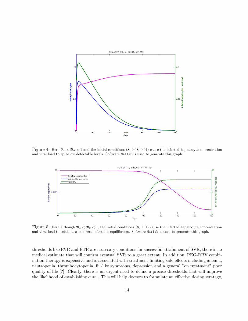
Figure 4: Here Rc < R0 < 1 and the initial conditions (8, 0.08, 0.01) cause the infected hepatocyte concentrationand viral load to go below detectable levels. Software Matlab is used to generate this graph.

Figure 5: Here although Rc < R0 < 1, the initial conditions (8, 1, 1) cause the infected hepatocyte concentrationand viral load to settle at a non-zero infectious equilibrium. Software Matlab is used to generate this graph.

thresholds like RVR and ETR are necessary conditions for successful attainment of SVR, there is nomedical estimate that will confirm eventual SVR to a great extent. In addition, PEG-RBV combi-nation therapy is expensive and is associated with treatment-limiting side-effects including anemia,neutropenia, thrombocytopenia, flu-like symptoms, depression and a general ”on treatment” poorquality of life [?]. Clearly, there is an urgent need to define a precise thresholds that will improvethe likelihood of establishing cure . This will help doctors to formulate an effective dosing strategy,

14

Nl'=O. \I4~ /, ( I U, III '/U )=(8, .lJ~ .lJ1)

""l-------_c~------_c,~ooo-------c,c~~:'':':~~ .... ." ,'.~"" ...... ~ d~~s

"'

~ • , • " ~

0.05 !

~

FD=D.9437, (TO, IJ , V1J)=(a, .15, .10)

" ~~~==F=~=:::::r:::::::::-'----------'----------'----I ---- healthy hepatocytes

w

---- infect ed hepatocytes ---- ,; ralload

[ } 0.0074

00 '00 '''' '" ,m ,:S days

-

:

[ } TI

~

Figure 6: Here R0 < Rc, the initial conditions (8, 1, 1) cause the infected hepatocyte concentration and viral loadto settle at a non-zero infectious equilibrium. Software Matlab is used to generate this graph.

Figure 7: Here R0 > 1 and the initial conditions (8, 0.01, 0.01) cause the infected hepatocyte concentration andviral load to go to a non-zero infectious equilibrium. Software Matlab is used to generate this graph.

take precautions against possible drug related toxicities and in general help patients to take aninformed decision about whether they want to go through the financial and physical perils of theupcoming 24 or 48 weeks of rigorous treatment.

Mathematical modeling has emerged as an important tool in medicine. Models of HCV infectionhave been effectively used to predict SVR (8-9) and to assess factors associated with favorableresponses. Viral and pharmacokinetic studies using mathematical models have shed light on our

15

understanding of HCV pathobiology and standardizing its treatment [?, ?]. In aggregate, thesestudies have contributed enormously to improve patient care. In this paper the four distinct patientprofiles were generated giving an idea of the functional property of the sub-clinical threshold. Itmight be possible to calculate the sub-clinical threshold using Rcrit, the lower boundary of thebistability region. The age of infection model with comparable dynamics should allow study of widerange of HCV patients under various assumptions hence leading to more precision in formulatingtreatment strategies.

For future work, I would like to replicate a wide range of HCV infected patient profiles from realpatient data and investigate the presence of the sub-clinical threshold. I would further like to studythe effects of different treatment regimes on each typical profile and include drug-related toxicitiesdue to adequate antiviral dosing, to find optimal individualized and therapeutic solutions.

5 Acknowledgements

I would like to thank Dr. Carlos Castillo-Chavez and Dr. Maia Martcheva for making this researchpossible. I thank Dr. Anuj Mubayi for his help and guidance. I would also thank Dr. ChristopherKribs-Zaleta and Dr. Marco Harrera for their support.

This MTBI project has been partially supported by grants from the National Science Foundation(NSF - Grant DMPS-0838704), the National Security Agency (NSA - Grant H98230-09-1-0104),the Alfred P. Sloan Foundation and the Office of the Provost of Arizona State University.

6 Appendix

6.1 Analysis of Age of Infection Model

Observation 3. The infection free equilibrium is locally asymptotically stable for R0 < 1 andunstable for R0 > 1.

To investigate the stability of the disease free equilibrium we introduce the following perturba-tions.

T (t) = T ∗ + x(t)i(τ, t) = y(τ, t)V (t) = z(t)

Now substituting this in the system 2 and applying the conditions from disease-free equilibrium

16

we get the following system.

dx

dt= r1x

(1− T ∗0

Tmax

)− dx− βT ∗0 z − r1T ∗0

x+ Y

Tmax∂y

∂t+∂y

∂τ= −δ(τ)y(τ, t) (28)

dz

dt=

∫ ∞0

p(τ)y(τ, t)dτ − cz

y(0, t) = βT ∗0 z +(

1− T ∗0Tmax

)∫ ∞0

r2(τ)y(τ, t)dτ

where,

Y (t) =∫ ∞

0y(τ, t)dτ.

Now we look for exponential solutions of the form

x(t) = eλtx

y(τ, t) = eλty(τ)z(t) = eλtz,

where λ is a constant. Substituting this we get the following system.

λx = r1x

(1− T ∗0

Tmax

)− dx− βT ∗0 z − r1T ∗0

x+ Y

Tmax

λy +dy

dτ= −δ(τ)y(τ) (29)

λz =∫ ∞

0p(τ)y(τ)dτ − cz

y(0) = βT ∗0 z +(

1− T ∗0Tmax

)∫ ∞0

r2(τ)y(τ)dτ

We solve the second differential equation to get,

y(τ) = y(0)e−λτe−∫ τ0 δ(η)dη

Using this we solve the third equation giving this expression for z,

z = y(0)Pλc+ λ

,

where,

17

P (λ) =∫ ∞

0p(τ)e−λτe−

∫ τ0 δ(η)dηdτ.

Now canceling out y(0) from the last equation in system (29) we get the following characteristicequation,

1 =βT ∗0λ+ c

Pλ +(

1− T ∗0Tmax

)R2λ

where,

R2λ =∫ ∞

0r2(τ)e−λτe−

∫ τ0 δ(η)dηdτ.

Now we define,

G(λ) :=βT ∗0λ+ c

Pλ +(

1− T ∗0Tmax

)R2λ. (30)

Differentiating with respect to λ we get,

G′(λ) = − βT ∗0λ+ c

λPλ −βT ∗0

(λ+ c)2Pλ −

(1− T ∗0

Tmax

)λR2λ

< 0, ∀λ

If we consider λ as a real variable we get that G(λ) is a decreasing function of λ with

limλ→∞

G(λ) = 0

Thus, if G(0) > 1 then G(λ) will definitely intersect G(λ) = 1 at least once. That would implythat the infection free equilibrium will become unstable.

Now if G(0) < 1, G(λ) = 1 does not have any real solutions. In that case, we explore the signof the real part of the solution of λ in the complex field. If possible, let λ = a+ ib, where a > 0.

|G(λ)| ≤ βT ∗0|λ+ c|

|Pλ|+(

1− T ∗0Tmax

)|R2λ|

≤ βT ∗0Reλ+ c

PReλ +(

1− T ∗0Tmax

)R2Reλ

≤ βT ∗0cP ∗ +

(1− T ∗0

Tmax

)R∗2

= G(0)< 1

Here, PReλ and R2Reλ are the values of Pλ and R2λ at λ = a respectively. We equate λ to 0to get the last inequality, giving us G(0). Thus, G(λ) = 1 does not have any solutions with the

18

Reλ ≥ 0. Thus, here the Infection free equilibrium is locally asymptotically stable. Thus, sinceG(0) < 1 is the criterion for local stability of the infection free equilibrium, we define, G(0) as thebasic reproduction number, R0.

R0 =βT ∗0cP ∗ +

(1− T ∗0

Tmax

)R∗2.

6.2 Analysis of ODE Model

Proof of Observation (1).First we calculate limI→F (I)∞ .

F (I) =β

δf(I) +

r2δ

(1− f(I) + I

Tmax

)− δ (31)

≤ βTmaxδ− r2I

δTmax, (32)

since, f(I)Tmax

< 1 at any moment of time, we have

limI→∞

F ′(I)→ −∞.

When, R0 > 1, i. e. F (0) > 1, F (I) can intersect F = 1 only odd number of times, since F (I)has to eventually decrease. Moreover, since from previous computations we see that I has atmost2 solutions, we conclude that, under this case, there exists a unique endemic equilibrium.

But when, R0 < 1, we consider 2 possible scenarios.If we have β− r2 > 0, we have from Equation (21) that F ′(I) < 0, for all I, since f ′(I) < 0, for

all I also, from Equation (20). Thus, F (I) does not intersect F = 1, hence no endemic equilibriumexists.

But if we have β − r2 < 0, we may expect the existence of two endemic equilibria.Stability of Infection Free EquilibriumTo linearize the ordinary differential equation system we construct the Jacobian and simplify

certain terms.

J =

−sT− r1T

Tmax− λ − r1T

Tmax−βT

βV − r2ITmax

r2

(1− T+I

Tmax

)− r2

TmaxI − δ − λ βT

0 p −c− λ

At the Infection free equilibrium (T 0, I0, V 0) the Jacobian reduces to,

J(T 0,I0,V 0) =

− sT 0− r1T 0

Tmax− λ − r1T 0

Tmax−βT 0

0 r2

(1− T 0

Tmax

)− δ − λ βT 0

0 p −c− λ

19

Thus the first eigenvalue is

λ = − sT− r1T

Tmax

is always negative, owing to the positivitity of our parameters. In the remaining 2×2 matrix, thetrace,

trJ(T 0,I0,V 0) = r2

(1− T 0

Tmax

)− δ − c

is negative and the determinant,

detJ(T 0,I0,V 0) = c

(r2

(1− T 0

Tmax

)− δ)− pβT 0

For the Infection free equilibrium to be stable we require the determinant to be positive. Hence,we derive the following condition.

βp

cδT 0 +

r2δ

(1− T 0

Tmax

)< 1,

giving us Basic reproduction number.Now going back to the Jacobian, J we investigate the stability of the endemic equilibriums.

First we define the following,

φ1 =s

T− r1T

Tmax

φ2 =βp

cδT +

r2Tmax

I

φ3 = c

We note that φ1, φ2, φ3 are all positive.Then the determinant of the Jacobian can be reduced to be,

λ3 +A1λ2 +A2λ+A3 = 0

where,

A1 = (φ1 + φ2 + φ3)

A2 =(φ1φ2 + φ2φ3 + φ3φ1 − pβT +

r1T

Tmax

(βp

c− r2Tmax

)I

)A3 = φ1φ2φ3 − pβT +

r1T

Tmax

(βp

c− r2Tmax

)Ic+ βp

(βp

c− r2Tmax

)IT

20

It can be easily verified that A1, A2 is always positive and

A3 > 0whenF ′(I1) < 0

A3 < 0whenF ′(I1) > 0

Now applying the Routh-Hurwitz Criterion we show that, under the conditions for backwardbifurcation we have that I1 is unstable and I2 is locally asymptotically stable in the bistabilityregion.

21