1

Time Series Sales Forecasting James J. Pao*, Danielle S. Sullivan**

*jpao@stanford.edu, **danielle.s.sullivan@gmail.com

Abstract—The ability to accurately forecast data is highly desirable in a wide variety of fields such as sales, stocks, sports performance, and natural phenomena. Presented here is a study of several time series forecasting methods applied to retail sales data, comprising weekly sales figures from various Walmart department stores across the United States over a period of approximately 2 and a half years. Significant surges in sales are noticeable in the data during pre-holiday and holiday weeks, which present a challenge for any developed forecasting models. The prediction models implemented herein are regression decision trees, Seasonal-Trend Decomposition using Loess and Autoregressive Integrated Moving-Average (STL + ARIMA) models, and time-lagged feed-forward neural networks (FFNNs). In particular, the STL + ARIMA and the time-lagged FFNN’s performed reasonably well in forecasting the weekly sales data. The best FFNN implementation, using a time-lag value d = 4 and mean weekly sales as inputs, achieved a mean absolute error of 1252. Weekly sales for the store departments are in the tens of thousands. It is also notable that the results achieved by the time-lagged FFNN’s did not require any deseasonalizing of the sales data, indicating that neural networks may be able to effectively detect and consider any seasonality during training and prediction.

————————————————————————

1 INTRODUCTIONN a world today where competitive margins are becoming increasingly narrower and actions

must be decisive yet informed, the ability to accu-rately make forecasts is of premier importance. This is certainly true in the forecasting of numeri-cal data such as the health of a country’s economy or the movements of a stock market from day to day. Forecasting is even beneficial in domains such as environmental monitoring or sports perfor-mance, and, accordingly, much forecasting work has been done across a broad swath of exciting fields and disciplines.

A more traditional yet still thoroughly compel-ling application of forecasting is sales prediction, which is the focus of this work. As markets become more and more global and competition is ruthless, optimizing an organization’s operational effi-ciency is of premium importance. When compa-nies must spread their resources broadly and con-sumers have a surfeit of choices, every advantage a company can squeeze out will make a difference. If a company can match the demand of a product with just the right amount of supply, then there will be no lost sales due to a lack of inventoy as well as no costs from overstocking. Sales forecast-ing uses patterns gleaned from historical data to predict future sales, allowing for informed courses-of-action such as allocating or diverting existing inventory, or increasing or decreasing fu-ture production.

This work investigates the performance of a va-riety of predictive models for the application of de-partmental sales forecasting. As a baseline method,

a regression decision tree is implemented. Then, the more sophisticated models of Seasonal-Trend Decomposition using Loess and Autoregressive Integrated Moving-Average (STL + ARIMA) and feed-forward neural networks using time-lagged inputs were used.

2 RELATED WORK Two currently popular approaches to nonlinear time series prediction problems are statistical ap-proaches using ARIMA and machine learning ap-proaches using Artificial Neural Networks (ANNs). ANNs have shown to perform well in time series forecasting because of their ability to accurately represent non-linear data [1]. Both of these approaches have had success when applied to sales forecasting and stock predictions [2]. When applied to financial data, the ARIMA model is able to leverage the fact that financial time series data is generally related to past values [3]. Provided there are no sudden changes in value or behavior, an ARIMA model will also be very effec-tive for financial time series forecasting [4]. In his 2010 paper Adebiyi [4] applies the ARIMA model to accurately forecast the Nokia stock prices. It is important to note that the linear assump-tions of the ARIMA model have resulted in poor forecasting models in cases of stock price predic-tion when the dataset includes values coming into and coming out of an economic recession (chang-ing properties).

I

2

In a separate paper Adebiyi [2] implements an ANN model and an ARIMA model to to predict Dell stock prices. In his model comparison, the ANN slightly outperforms the ARIMA model. Adebiyi attributes this partially to the fact that the ARIMA model assumes that the times series is generated from a linear process.

3 DATASET The dataset used was provided by Walmart Inc., an American multinational retail corporation, for a 2014 data science competition (Kaggle).

The dataset contains historical weekly sales data from 45 Walmart department stores in different re-gions across the United States. The training set has 421,570 samples. Each sample has the following features: departmental weekly sales, the associated department (81 departments, each listed as a num-ber), the associated store (listed as a number), the store type, the date of the week’s start day, a flag indicating if the week contains a major holiday (Super Bowl, Labor Day, Thanksgiving, Christ-mas).

Also supplied is a corresponding set of features for each week-store combination which includes temperature, fuel price, CPI, unemployment rate, and promotional markdown data.

There is no publicy available test set. Specifi-cally, the ground-truth values for the test set are not available, so assessing each model against the official test set must be done by making test pre-dictions and submitting to Kaggle’s online plat-form. Hold-out sets are generated from the pro-vided training samples for local validation, but for some models (namely the neural networks) these hold-out sets are also used as the test-sets for rea-sons explained later.

4 METHODS Three primary prediction models were developed in this study: regression decision trees, STL + ARIMA, and time-lagged feed-forward neural net-works. Other algorithms such as the k-nearest neighbors (KNN) clustering and naïve Bayes algo-rithsm were investigated, but results were poor and insights were insignificant so they will not be discussed herein. 4.1 Regression Decision Tree As a baseline method, a decision tree utilizing the features provided in the dataset was implemented. This model was chosen as a baseline since it is eas-ily implemented and leveraged the way the pro-vided data was organized.

The splitting attributes chosen were week num-ber, store number, department number, the holiday flag, and the store size. The tree was implemented using MATLAB’s fitrtree function, which follows the Classification and Regression Tree (CART) al-gorithm [5], choosing splits to maximize the cho-sen split-criterion gain. In the MATLAB imple mentation using CART, mean-squared error is cal-culated for the responses and splits among the data are done to maximize mean-squared error reduc-tion.

4.2 STL + ARIMA A widely used approach to modeling time series data is the Seasonal-Trend Decomposition using Loess and Autoregressive Integrated Moving-Av-erage (STL + ARIMA) method.

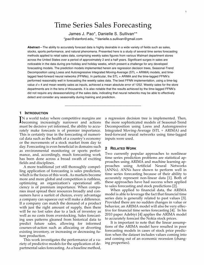
The STL + ARIMA model extracts the trend, seasonality and remainder components of the time series data and then implements the ARIMA model to forecast the reaminder component of the decomposed time series data. Then the seasonality componenet is added back in to complete the pre-diction. The STL method used here is an additive decomposition technique, as the seasonal compo-nent of the sales data does not vary greatly with trend [6]. In fact, there does not appear to be much trend in the sales data at all. A sample plot of the components of a weekly sales time series are shown in Figure 1.

Fig 1. Sample plots of observed, trend, seasonal, and remainder components after additive decomposition

for a weekly sales time series

To be clear, each component of time series data as mentioned above is described below in more de-tail.

· Trend components are long-term non-sea sonal patterns in the data, such an upward lin ear trend in sales per week. · Seasonal components are periodic patterns in the time series data. For the given dataset, which entails predicting weekly sales values, there is likely to be a seasonal componenet with a period of 52. Examples of seasonal com ponents in our data include spikes in sales within a school supplies related department in the month of August, or spikes in sales of toys

PAO, J., SULLIVAN, D. - TIMES SERIES SALES FORECASTING 3

the weeks preceding Christmas. · Remainder components includes any changes in the data not captured in the trend or seasonal components. These are random fluctuations in the weekly sales from one week to another. In the decomposition of the data, the Local Re-gression (Loess) smoothing technique is applied, determining how the cycle subseries (distinct weeks within the 52-week period) are combined to calculate the seasonal componenet of the data. The higher the degree of smoothing applied, the closer in value the seasonal decomposition comes to an average over each cycle subseries. Higher degrees of smoothing do not allow for variation between cycle subsreries in different periods. Af-ter the decomposition of the time series data, the seasonal and trend data is extended to forecast the seasonal and trend components of the test data. To finish the additive prediction model, ARIMA is applied to forecast the remainder com-ponent of the data. ARIMA accounts for the relationship between a variable’s value in one period to the past values (autoregressive) and the ranodom errors of the past estimated values from previous periods (moving-average). The algorithm also applies a differecing technique to transform the data into stationary data if necessary. The equation defin-ing ARIMA is shown below:

In this equation, p is the number of terms in-cluded in the autoregressive moving-window (number of past time-steps to include) and q is the number of past residuals included in the moving-average. Finally, it is important to note that ARIMA requires stationary data [7] (constant mean and variance over time) so differencing (in-tegration) of the data may be needed. For exam-ple, in differencing the data, the post-differencing value at time t can be calculated as the value at time t minus the value from the previous time-step, t-1. The degree of differencing is specified by the d parameter in the ARIMA equation. The STL + ARIMA model was implemented in R, and the optimal values for p, q, and d were cho-sen using the Bayesian Information Criterion (BIC) for each potential model. BIC is a measure that quantifies the reward associated with good-ness of fit of the model and a penalization for overfitting the model (a large p+q). 4.3 Time-lagged Feed-Forward Neural Network

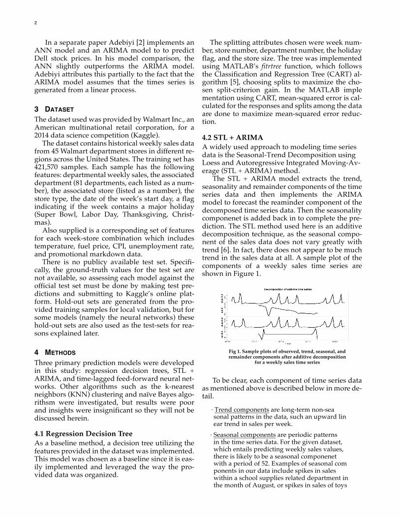
Neural networks are very powerful machine learn-ing models that are highly flexible universal ap-proximators [6], needing no prior assumptions during model construction. Neural networks per-form end-to-end learning when being trained, de-termining the intermediate features without any user-feedback [8]. It has been proposed by multiple sources that neural networks can model time series data effec-tively, even without the need for data prepro-cessing such as deseasonalizing [9]. The neural networks implemented here are standard feed-forward neural networks (FFNNs), which have all layer outputs heading in the same direction (no loops). The neural networks all also have a single hidden layer. The inputs are selected to be a combination of time-lagged data and mean weekly sales. Specifically, using d lagged values to predict a weekly sales value at time t, the inputs will be the weekly sales values for times t-1 through t-d as well as the mean of the weekly sales values for the week number that timestep t corre-sponds to. FFNNs with varying d values (d=1, d-2, d-4, d=6) are considered and reported. The FFNN design used is shown in Figure 2, where xMWS is the mean weekly sales for the week corresponding to time t.

Fig 2. Time-lagged feed-forward neural network design implemented in this work

All implemented FFNNs use the sigmoid function as the activation function for the hidden layer. Three different backpropogation algorithms are considered: the Levenberg-Marquardt (LM) algorithm, the Scaled Conjugate Gradient (SCG) algorithm, and the Resilient Backpropogation (RP) algorithm. All neural networks were imple-mented using MATLAB’s Neural Network toolbox. During training, 75% of training samples was used in the training subset and 25% was used for the cross-validation subset. 4.4 Implementation Strategy As noted before, the test set’s ground-truth values are not made publicly available. Therefore, the FFNN implementation could not be tested using Kaggle’s provided test set (which only has features for each sample such as department number, store number, week number) since the FFNN uses time-

4

lagged inputs. As the decision tree and the STL + ARIMA models do not require the ground-truth values of the test set, these models were tested using Kaggle’s online submission platform and com-pared to online baselines. The scoring online is done using a weighted mean absolute error (WMAE). Since the test set is designed by Kaggle and can encompass any department, store, or week, a separate STL + ARIMA model was created for each store and department combination, and the appropriate one was used for each sample in the test set. For the FFNN testing, a local test set was se-lected from the tail of the training set. FFNNs were implemented only for the Store 1 – Department 1 combination since all model selection and testing must be done locally. The number of weeks chosen for the test set was the last 33 weeks out of 143 weeks available in the training set, as this was small enough to allow for enough weeks for train-ing and cross-validation but also large enough to include some holiday sales spikes which are of in-terest. Performance assessment was done using mean absolute error (MAE).

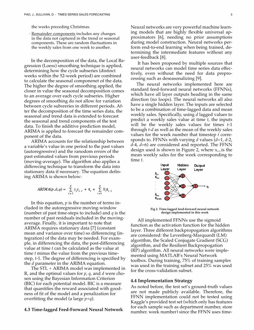
5 RESULTS Using the decision tree model on Kaggle’s test set resulted in a WMAE score of 4384.4. This was con-sidered an acceptable baseline, as the winning sub-missions for the Kaggle competition was approxi-matel 2300. A submission with all 0’s for the pre-diction results in a WMAE of approximately 21,000. As the STL + ARIMA model also does not need the ground-truth values of the test set, it was used to predict values for the test set and was tested us-ing Kaggle’s online submission. The STL + ARIMA model performed very well, achieving a WMAE of 2875.6. This score was within 500 points of the win-ning Kaggle submission, and a significant reason for the disparity is likely due to the fact that the STL + ARIMA model does not account for the fact that there is a large sales spike preceeding Easter for many departments and that Easter is a moving holiday (it occurs on a different week each year of the training and test data). As an example, shown in Figure 3 is plot of the training values of weekly sales for store 1, department 1, along with the pre-dicted values from the STL + ARIMA model. The vertical bars represent holiday markers, where lime green is Labor Day, light brown is Thanksgiv-ing, dark brown is Christmas, sea-foam green is Super Bowl, and magenta is Easter. Note that

Easter is inconsistent for each year.

Fig 3. Training and predicted weekly sales values from the STL +

ARIMA model for Store 1, Department 1

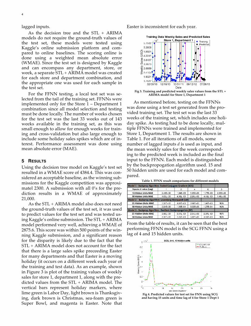
As mentioned before, testing on the FFNNs was done using a test set generated from the pro-vided training set. The test set was the last 33 weeks of the training set, which includes one holi-day spike. As testing had to be done locally, mul-tiple FFNNs were trained and implemented for Store 1, Department 1. The results are shown in Table 1. For all iterations of all models, some number of lagged inputs d is used as input, and the mean weekly sales for the week correspond-ing to the predicted week is included as the final input to the FFNN. Each model is distinguished by the backpropogation algorithm used. 15 and 50 hidden units are used for each model and com-pared.

Table 1. FFNN result comparisons for different models

From the table of results, it can be seen that the best performing FFNN model is the SCG FFNN using a lag of 4 and 15 hidden units.

Fig 4. Predicted values for test set for FNN using SCG

and having 15 units and time lag of 4 for Store 1 Dept 1

PAO, J., SULLIVAN, D. - TIMES SERIES SALES FORECASTING 5

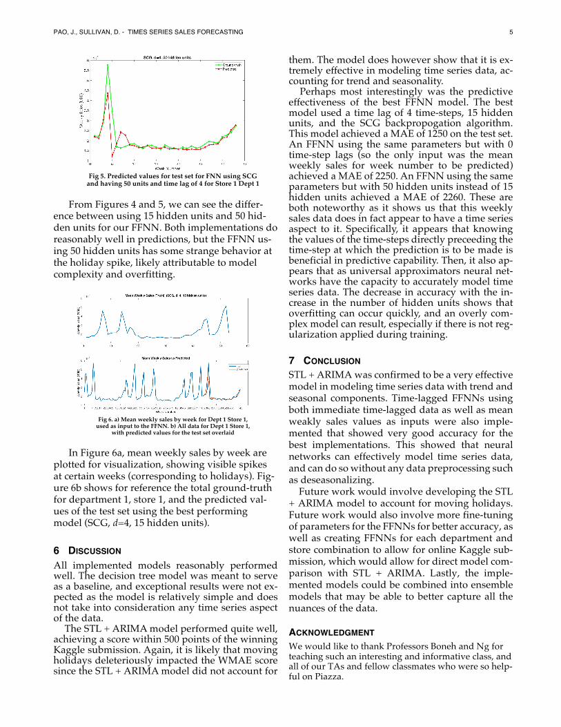
Fig 5. Predicted values for test set for FNN using SCG

and having 50 units and time lag of 4 for Store 1 Dept 1

From Figures 4 and 5, we can see the differ-ence between using 15 hidden units and 50 hid-den units for our FFNN. Both implementations do reasonably well in predictions, but the FFNN us-ing 50 hidden units has some strange behavior at the holiday spike, likely attributable to model complexity and overfitting.

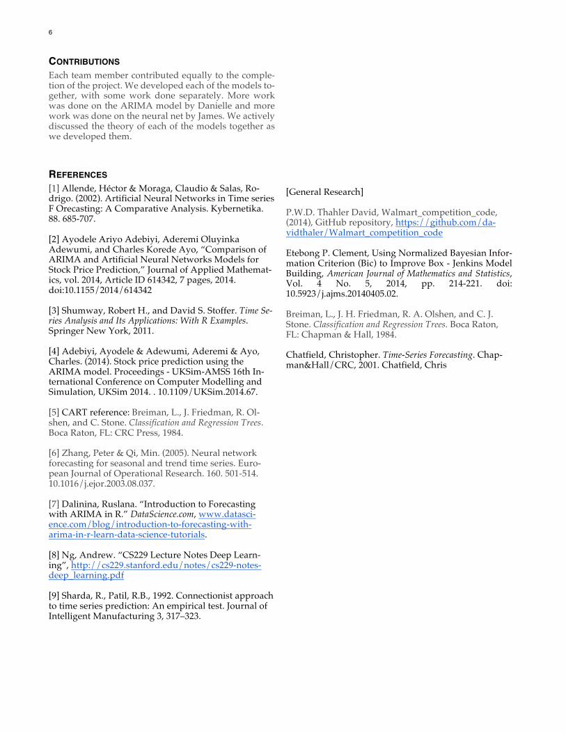
Fig 6. a) Mean weekly sales by week for Dept 1 Store 1,

used as input to the FFNN. b) All data for Dept 1 Store 1, with predicted values for the test set overlaid

In Figure 6a, mean weekly sales by week are plotted for visualization, showing visible spikes at certain weeks (corresponding to holidays). Fig-ure 6b shows for reference the total ground-truth for department 1, store 1, and the predicted val-ues of the test set using the best performing model (SCG, d=4, 15 hidden units).

6 DISCUSSION All implemented models reasonably performed well. The decision tree model was meant to serve as a baseline, and exceptional results were not ex-pected as the model is relatively simple and does not take into consideration any time series aspect of the data.

The STL + ARIMA model performed quite well, achieving a score within 500 points of the winning Kaggle submission. Again, it is likely that moving holidays deleteriously impacted the WMAE score since the STL + ARIMA model did not account for

them. The model does however show that it is ex-tremely effective in modeling time series data, ac-counting for trend and seasonality.

Perhaps most interestingly was the predictive effectiveness of the best FFNN model. The best model used a time lag of 4 time-steps, 15 hidden units, and the SCG backpropogation algorithm. This model achieved a MAE of 1250 on the test set. An FFNN using the same parameters but with 0 time-step lags (so the only input was the mean weekly sales for week number to be predicted) achieved a MAE of 2250. An FFNN using the same parameters but with 50 hidden units instead of 15 hidden units achieved a MAE of 2260. These are both noteworthy as it shows us that this weekly sales data does in fact appear to have a time series aspect to it. Specifically, it appears that knowing the values of the time-steps directly preceeding the time-step at which the prediction is to be made is beneficial in predictive capability. Then, it also ap-pears that as universal approximators neural net-works have the capacity to accurately model time series data. The decrease in accuracy with the in-crease in the number of hidden units shows that overfitting can occur quickly, and an overly com-plex model can result, especially if there is not reg-ularization applied during training.

7 CONCLUSION STL + ARIMA was confirmed to be a very effective model in modeling time series data with trend and seasonal components. Time-lagged FFNNs using both immediate time-lagged data as well as mean weakly sales values as inputs were also imple-mented that showed very good accuracy for the best implementations. This showed that neural networks can effectively model time series data, and can do so without any data preprocessing such as deseasonalizing. Future work would involve developing the STL + ARIMA model to account for moving holidays. Future work would also involve more fine-tuning of parameters for the FFNNs for better accuracy, as well as creating FFNNs for each department and store combination to allow for online Kaggle sub-mission, which would allow for direct model com-parison with STL + ARIMA. Lastly, the imple-mented models could be combined into ensemble models that may be able to better capture all the nuances of the data.

ACKNOWLEDGMENT We would like to thank Professors Boneh and Ng for teaching such an interesting and informative class, and all of our TAs and fellow classmates who were so help-ful on Piazza.

6

CONTRIBUTIONS Each team member contributed equally to the comple-tion of the project. We developed each of the models to-gether, with some work done separately. More work was done on the ARIMA model by Danielle and more work was done on the neural net by James. We actively discussed the theory of each of the models together as we developed them.

REFERENCES [1] Allende, Héctor & Moraga, Claudio & Salas, Ro-drigo. (2002). Artificial Neural Networks in Time series F Orecasting: A Comparative Analysis. Kybernetika. 88. 685-707. [2] Ayodele Ariyo Adebiyi, Aderemi Oluyinka Adewumi, and Charles Korede Ayo, “Comparison of ARIMA and Artificial Neural Networks Models for Stock Price Prediction,” Journal of Applied Mathemat-ics, vol. 2014, Article ID 614342, 7 pages, 2014. doi:10.1155/2014/614342 [3] Shumway, Robert H., and David S. Stoffer. Time Se-ries Analysis and Its Applications: With R Examples. Springer New York, 2011. [4] Adebiyi, Ayodele & Adewumi, Aderemi & Ayo, Charles. (2014). Stock price prediction using the ARIMA model. Proceedings - UKSim-AMSS 16th In-ternational Conference on Computer Modelling and Simulation, UKSim 2014. . 10.1109/UKSim.2014.67. [5] CART reference: Breiman, L., J. Friedman, R. Ol-shen, and C. Stone. Classification and Regression Trees. Boca Raton, FL: CRC Press, 1984. [6] Zhang, Peter & Qi, Min. (2005). Neural network forecasting for seasonal and trend time series. Euro-pean Journal of Operational Research. 160. 501-514. 10.1016/j.ejor.2003.08.037. [7] Dalinina, Ruslana. “Introduction to Forecasting with ARIMA in R.” DataScience.com, www.datasci-ence.com/blog/introduction-to-forecasting-with-arima-in-r-learn-data-science-tutorials. [8] Ng, Andrew. “CS229 Lecture Notes Deep Learn-ing”, http://cs229.stanford.edu/notes/cs229-notes-deep_learning.pdf [9] Sharda, R., Patil, R.B., 1992. Connectionist approach to time series prediction: An empirical test. Journal of Intelligent Manufacturing 3, 317–323.

[General Research] P.W.D. Thahler David, Walmart_competition_code, (2014), GitHub repository, https://github.com/da-vidthaler/Walmart_competition_code Etebong P. Clement, Using Normalized Bayesian Infor-mation Criterion (Bic) to Improve Box - Jenkins Model Building, American Journal of Mathematics and Statistics, Vol. 4 No. 5, 2014, pp. 214-221. doi: 10.5923/j.ajms.20140405.02. Breiman, L., J. H. Friedman, R. A. Olshen, and C. J. Stone. Classification and Regression Trees. Boca Raton, FL: Chapman & Hall, 1984. Chatfield, Christopher. Time-Series Forecasting. Chap-man&Hall/CRC, 2001. Chatfield, Chris