Embed Size (px)
Citation preview
1
Time-series regression models to study the short-term effects
of environmental factors on health*
Aurelio Tobías† and Marc Saez
ψ
Departament d’Economia,
Universitat de Girona
Girona, March 2004
Abstract
Time series regression models are especially suitable in epidemiology for evaluating
short-term effects of time-varying exposures on health. The problem is that potential for
confounding in time series regression is very high. Thus, it is important that trend and
seasonality are properly accounted for. Our paper reviews the statistical models commonly
used in time-series regression methods, specially allowing for serial correlation, make them
potentially useful for selected epidemiological purposes. In particular, we discuss the use of
time-series regression for counts using a wide range Generalised Linear Models as well as
Generalised Additive Models. In addition, recently critical points in using statistical
software for GAM were stressed, and reanalyses of time series data on air pollution and
health were performed in order to update already published. Applications are offered
through an example on the relationship between asthma emergency admissions and
photochemical air pollutants in Madrid for the period 1995-1998, of how these methods are
employed.
Keywords: Time-series, Poisson, GLM, GAM, autocorrelation, overdispersion, air
pollution.
JEL classification: C51, C53, Q51, Q54.
* We want to thank comments and advice from José Ramón Banegas, Iñaki Galán, Julio Díaz, María
Antonia Barceló and Ricardo Ocaña. We also acknowledge the following institutions to provide data: Red
Palinológica de la Consejería de Sanidad de la Cominidad de Madrid, Departamento de Control de
Contaminación Atmosférica del Ayuntamiento de Madrid, Subdirección General de Calidad Ambiental
del Ministerio de Medio Ambiente, Programa Regional de Prevención y Control del Asma and Hospital
Gregorio Marañón. This study was funded by the Comisión Asesora del Programa Regional de
Prevención y Control del Asma de la Comunidad de Madrid and Aurelio Tobías was enjoying a
postgraduate fellowship of Universidad Autónoma de Madrid. † Address: Department of Statistics and Econometrics, Universidad Carlos III de Madrid, 28903-Getafe.
E-mail: [email protected] ψ Address: Departament d’Economia. Universitat de Girona, Campus de Montilivi, 17071 Girona. E-mail:
2
1. Introduction
In time series regression dependent and independent variables are measured over time,
and we would like to model the possible relationship between these through regression
methods. Examples of epidemiological time series studies are the studies of the
relationship between mortality and air pollution (Katsouyanni et al. 1996, Ballester et al.
1999, Samet et al. 2000, Katsouyanni et al. 2002a), hospital admissions and air pollution
(Katsouyanni et al. 1996, Touloumi et al. 2003), mortality from sudden infant death
syndrome and environmental temperature (Campbell 1994) and atmospheric pressure
(Campbell et al. 2001), or infectious gastrointestinal illness (Schwartz et al. 1997) and
mortality (Braga et al. 2001) related to drinking water. However, various methods have
been used in these analyses, from linear (Hatzakis et al. 1986) to log-linear
(Mackenbach et al. 1992) and Poisson regression models (Schwartz et al. 1996), and
recently generalised additive models (Schwartz 1994, Kelsall et al. 1997).
Time series regression models are especially suitable in epidemiology for
evaluating short-term effects of time-varying exposures. Typically, a single population
is assessed with reference to its change over the time in the rate of any health outcome
and the corresponding changes in the exposure factors during the same period.
Covariates varying between subjects but not over time, for example sex, cannot
confound the associations and there are not considered. Furthermore, covariates that
may also vary within subjects, say sex or smoking habit, but whose daily variation is
unlikely to vary at same time with the exposure, can be excluded as confounders. The
problem is that the potential for confounding in time series regression is very high. It is
important that seasonality and trends are properly accounted for. Many variables either
simply increase or decrease over time, and so will be correlated over time (Yule 1926).
In addition many other epidemiological variables are seasonal, and this variation would
be present even if the factors were not causally related. Simply because the outcome
variable is seasonal, it is impossible to ascribe causality because of seasonality of the
predictor variable. For example, sudden infant deaths are higher in winter than in
summer, but this does not imply that temperature is a causal factor; there are many other
factors that might affect the result such as reduced daylight, or presence of viruses.
However, if an unexpectedly cold winter is associated with an increase in sudden infant
deaths, or very cold days are consistently followed after a short time by rises in the daily
sudden infant death rate, then causality may possibly be inferred (Campbell 1994).
The following paper reviews the statistical models which have commonly been
used in time series regression, specially allowing for serial correlation, which make
them potentially useful for selected epidemiological purposes. An application of how
these methods are employed is given by an example on the relationship between asthma
emergency room admissions and photochemical air pollutants in Madrid (Spain) (Galan
et al. 2003).
3
2. Regression model for counts
In the analysis of epidemiological time series data consisting of counts, the underlying
mechanism being modelled is a Poisson process with a homogeneous risk λ, i.e. the
expected number of counts on day t, to the underlying population is assumed. The
probability of yt occurrences on a given day t is defined by
( )!y
e|yprob
t
y
t
tλ=λ
λ−
(1)
The Poisson regression model assumes
( )
β+β= ∑
=
n
1i
tii0tt xexpx|yE (2)
where xt is the column vector of independent variables on day t with regression
coefficients β and yt is the dependent variable on day t.
The equation (2) could also be formulated as a Generalised Linear Model (GLM)
(McCullagh and Nelder 1989),
Link function
( )
( ) ∑=
β+β=µ
µ=n
1i
tii0t
ttt
xlog
x|yE
(3)
Variance function
( ) ttyV µ= (4)
The usefulness of Poisson regression in epidemiology is that it provides an
estimation of the relative risk (RR) as RRi=exp(βi) where βi is the regression coefficient
associated with a unit increment in a pollutant.
4
3. Misspecification in time series regression
3.1. Autocorrelation
A basic assumption of any regression analysis is that observations must be identically
independently distributed, that is xt and/or yt are not influenced by previous values, say
for example xt-1 and yt-1, respectively. Dealing with time series data this assumption is
usually broken. When the dependent variable, yt, is observed over time, usually all the
independent variables, xt, have a temporal structure. As a consequence, the observations
of the response have a temporal dependence, probably due to the effect of
misspecification, for instance omitted variables.
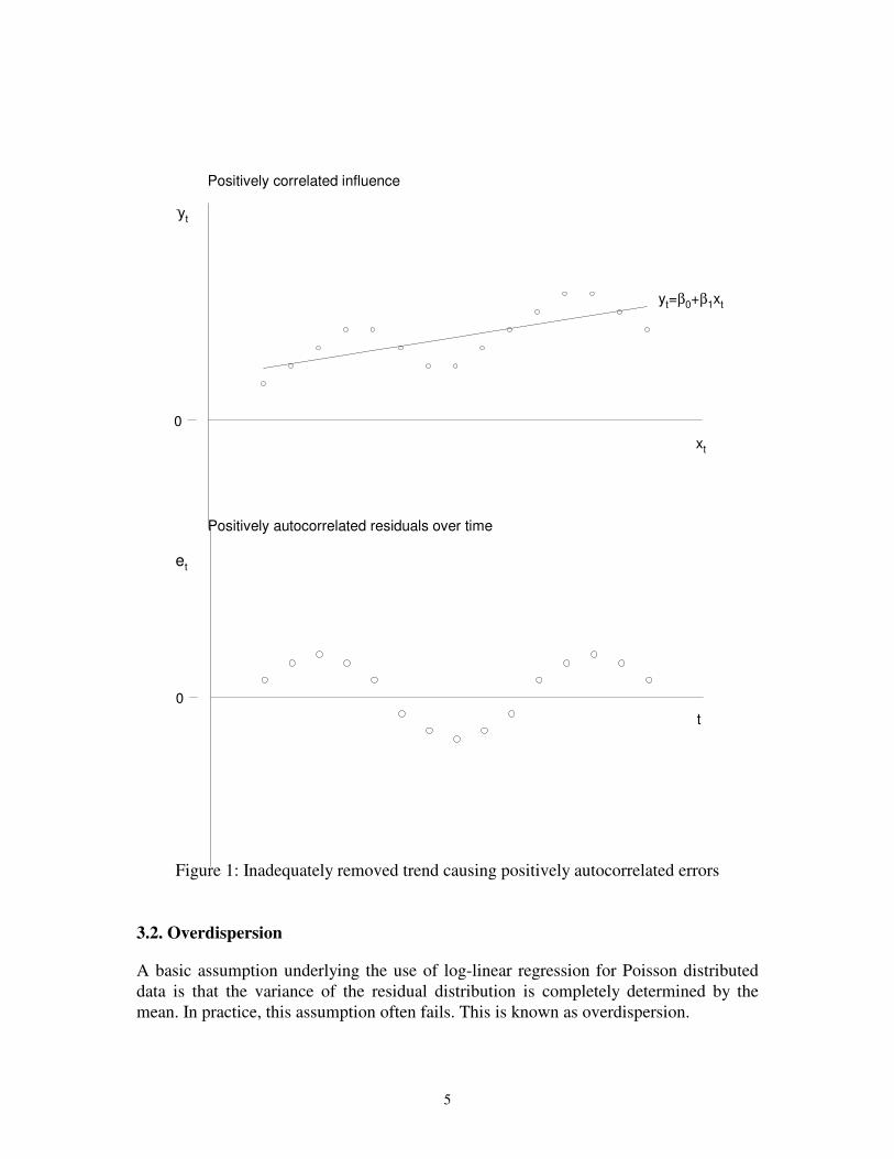
Figure 1 presents an example where a positively correlated influence causes
positively autocorrelated residuals. The possible relationship between xt and yt is
masked by a clear seasonal pattern in yt. When this relationship is isolated there remains
an autocorrelated structure for the residuals et. In fact, often when confounding factors
are correctly accounted for, the serial correlation of the residuals disappears; they appear
serially correlated because of the association with a time dependent predictor variable,
and so conditional on this variable the residuals are independent. This is particularly
likely for mortality data, where, except in epidemics, the individual deaths are unrelated.
However, if the model were correct, the residual autocorrelation should be
minimal since one death does not cause another. Thus residual autocorrelation maybe
implies confounding of air pollution associations due to unmeasured or missmodeled
variables. In fact, if the inclusion of known or potential cofounders fails to remove the
serial correlation of the residuals, then it is known that the estimation methods does not
provide valid estimates of the standard errors of the parameters (Campbell 1998). For
example, analysing the relationship between daily mortality and air pollutants the effects
of trend, weather and unusual events are not included in such relationship. These
variables are autocorrelated themselves and consequently the residuals will be
dependent. In the same way, the relationship between daily mortality and weather
temperature presents the typical V-shape (Saez et al. 1995). Low environmental
temperature implies high mortality and very high weather temperature is also related to
high mortality. Increasing temperature up to a certain point, however, reduces mortality.
If the regression does not account for this fact positive residuals will be followed by
other positive residuals and the same event occurs with negative residuals.
Thus, in time series regression one can often use conventional regression methods
followed by a check for the serial correlation of the residuals and need only proceed
further if there is clear evidence of a lack of independence.
5
0
et
t
Positively autocorrelated residuals over time
0
6
Positively correlated influence
xt
yt
yt=β0+β1xt
Figure 1: Inadequately removed trend causing positively autocorrelated errors
3.2. Overdispersion
A basic assumption underlying the use of log-linear regression for Poisson distributed
data is that the variance of the residual distribution is completely determined by the
mean. In practice, this assumption often fails. This is known as overdispersion.
6
In this case (4) could be replaced by
φµ=)y(V t (5)
where φ is an scalar capturing the over-dispersion (McCullagh and Nelder 1989).
4. Time series regression models for counts
4.1. Marginal and conditional models
A number of authors have distinguished marginal and conditional models (Fitzmaurice
1998). For a marginal model E(yt)=f(xt,xt-1,...,xt-τ) where the xt's are external time-
varying covariates. This is in contrast to a conditional model in which E(yt)=f(xt,xt-
1,...,xt-τ,yt-1,...,xt-υ), τ≥0, υ≥1, and the past values of the dependent variable are included
as new predictor variables. It has been argued that marginal models are rather artificial,
and give unlikely correlation structures. However, they are very useful for modelling
mean rates in populations. On the other hand, conditional models are useful for
modelling changes in individuals but are poor at determining relationships between the y
and x's variables because the parameters are not readily interpretable (Staneck et al.
1989).
4.2. Transitional models
Brumback et al. (2000) unifies the marginal and conditional extension of the GLM for
non-Gaussian time series under the heading of Transitional Regression Models (TRM).
These are non-linear regression models that can be written in terms of conditional
means and variances given past observations. The term transitional is used rather than
conditional to emphasise that the outcomes are ordered in time and that the conditioning
is on past outcomes only, and also to allude to the transitional probabilities of Markov
models. Rather than specifying the entire probability distributions of the transitions
between outcomes, the TRM parameterises the transitional means and variances.
Firstly, the simplest way to deal with those problems is to included lagged values
of the outcome as covariates in the model; an approach that could be called transitional
GLM (TGLM) (Brumback et al. 2000)
( ) ( )∑ ∑= =
−θ+β+β=µn
1i
k
1j
jtitjjiti0t y,xfxlog (6)
where fj are (known) functions of both, covariates and past responses, and θj denote
unknown parameters.
7
A slightly more sophisticated approach includes the case of standardised residuals
of earlier observations as covariates, the GLM with time series errors, GLM with TSE
(Schwartz et al. 1996)
∑ ∑= = −
−
υθ+β+β=µ
n
1i
k
1j jt
jt
jiti0t
ex)log( (7)
where ttt ye υ−= ,
β+β=υ ∑
=
n
1i
iti0t xexp . However, et could also be scaled by φ in
order to avoid for possible overdispersion.
Comparison between models could be done by using the Akaike Information
Criteria (AIC) (Akaike 1973)
AIC = D + 2df (8)
where D denotes the deviance, and df are the degrees of freedom for the model.
4.2. Generalised Additive Models
The Generalised Additive Models (GAM) extends the GLM by fitting non-parametric
functions (gi below) to estimate the relationships between the response and the
predictors (Hastie and Tibshirani, 1989)
( ) ( )∑=
+β=µn
1i
iti0t xglog (9)
Since these functions are unknown infinite dimensional parameters, we could
consider estimating them by using natural cubic smoothing splines (Wahba 1990, Green
and Silverman 1994). The amount of smoothing in the splines, technically the
approximate degrees of freedom, could be decided by means of the AIC
A spline with k degrees of freedom for a particular explanatory variable would be
similar to introducing k dummy variables for the covariate in the model, each one
corresponding to a time period of n/k, where n is the total number of days (Kelsall et al.
1997).
However, GAM models could also be formulated as transitional models (TGAM)
( ) ( ) ( )∑ ∑= =
−θ++β=µn
1i
k
1j
jtitjjiti0t y,xfxglog (10)
or as a GAM with TSE
8
( )∑ ∑= = −
−
υθ++β=µ
n
1i
k
1j jt
jt
jiti0t
exg)log( (11)
4.3. Exact GAM
While GAM has been the preferred method to model the relationship between health
outcome time series and exposures, mainly air pollutants and meteorological variables,
recent reports, however, have questioned the adequacy of its use for time series
epidemiological studies.
Dominici et al. (2002) have reported that in the standard case of studies looking
for the short-term health effects of air pollution where: a) regression coefficients are
very small and b) adjustment is made for at least two confounding factors using non-
parametric smoothing functions, estimated GAM models using the gam function in S-
Plus (Insightful Corporation, Seattle, WA, USA) may provide biased estimates of the
regression coefficients and their standard errors. This is due to the original default
parameters were inadequate to guarantee the convergence of the backfitting algorithm.
Although the defaults have recently been revised (Dominici et al 2002, Katsouyanni et
al. 2002b), a remaining and important problem is that S-Plus function gam calculates
the standard errors of the linear terms by effectively assuming that the smooth
component of the model is linear, resulting in an underestimation of uncertainty
(Chambers and Hastie 1992; Ramsay et al. 2003).
Briefly, an explicit version for the asymptotically exact covariance matrix of the
linear terms is HWH)ˆ(V 1−′=β (Hastie and Tibshirani 1990), where
( ){ } ( )SIWXXSIWXH1
−′−′=−
; X is a design matrix; W is diagonal in the final IRSL
weights; )z(CovW 1 =− ; z is the working response form the final version of the IRLS
algorithm (McCullagh and Nelder 1989); and S is the operator matrix that fits the
additive model involving the smooth terms in the model.
Because calculation of the operator matrix S can be computationally expensive,
the current version of the S-Plus function gam approximates ( ) 1
aug
'
augWXX)ˆ(V−
=β ;
where Xaug is the design matrix of the model augmented by the predictors used in the
smooth component (Hastie and Tibshirani 1990, Chambers and Hastie 1992). That is to
say, the asymptotic variance is approximated by effectively assuming that the smooth
component of the model is linear. In time series studies, the assumption of linearity is
inadequate, resulting in underestimation of the standard error of the linear term (Ramsay
et al. 2003). The degree of underestimation will tend to increase with the number of
degrees of freedom used in the smoothing splines, because a larger number of non-linear
terms is ignored in the calculations. Here, Dominici et al. (2003) re-define H as
( ){ } ( )WSXWXWSXWXXH1
−−′=−
and also provide exact details of the calculation
of an estimate of the asymptotic variance.
9
5. Example
5.1. Data
Asthma daily emergency room admissions to the Emergency Ward of the Gregorio
Marañón University Hospital, was studied for the period 1995-1998. The pollutants and
analytical methods used were: particulates measured as the daily average of NO2 and
average of maximum 8-hourly O3 values. Pollution data were obtained from the
automated network of the Madrid City Comprehensive Air-Pollution Monitoring,
Forecasting and Information. We used mean temperature and mean relative humidity as
registered at the Barajas meteorological observatory, situated 8 kilometres north-east of
the city. Information was also obtained on reported cases of acute respiratory infection
attended at the Gregorio Marañón Hospital Emergency Ward. Additional details have
been reported elsewhere (Galán et al. 2003).
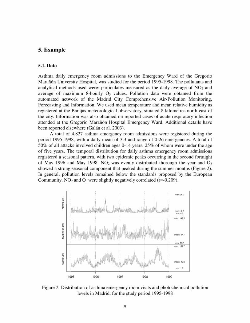
A total of 4,827 asthma emergency room admissions were registered during the
period 1995-1998, with a daily mean of 3.3 and range of 0-26 emergencies. A total of
50% of all attacks involved children ages 0-14 years, 25% of whom were under the age
of five years. The temporal distribution for daily asthma emergency room admissions
registered a seasonal pattern, with two epidemic peaks occurring in the second fortnight
of May 1996 and May 1998. NO2 was evenly distributed thorough the year and O3
showed a strong seasonal component that peaked during the summer months (Figure 2).
In general, pollution levels remained below the standards proposed by the European
Community. NO2 and O3 were slightly negatively correlated (r=-0.209).
1995 1996 1997 1998 1999
O3
(ma
x.8
h)
NO
2(m
ea
n.2
4h
)A
sth
ma
ER
min: 0.0
min: 1.9
min: 25.7
max: 26.0
max: 152.7
max: 147.5
mean: 3.3
mean: 45.8
mean: 67.1
Figure 2: Distribution of asthma emergency room visits and photochemical pollution
levels in Madrid, for the study period 1995-1998
10
5.2. Parametric modelling
For Poisson regression models we followed a standardised protocol (Katsouyanni et al.
1996) which has widely been applied in other multicentre studies (Ballester et al. 1999).
To control for unobserved covariates with a systematic behaviour in time we introduced
a linear and quadratic trends and dummy variables for each year to control for long
wavelength trends, sinusoidal terms to control for seasonality and dummy variables for
week days and public holidays to control for weekly variation. Covariates considered
were temperature and humidity; and daily reported cases of acute respiratory infection.
The variables included in the model were chosen individually, on the basis of their
respective levels of significance, and jointly on the basis of those that minimised the
AIC criterion. Once the best-fitted core model had been selected with the support of
Pearson residuals, we then tested for overdispersion using the overdispersion parameter,
and for residual autocorrelation using the simple (ACF) and partial autocorrelation
function (PACF) plots. Finally, four models were considered to assess for the
relationship between asthma emergency room admissions and photochemical air
pollutants: GLM, GLM corrected by overdispersion, TGLM, and GLM with TSE, where
the pollutants were next included on a linear basis, with assessment of lags up to the
fourth order.
5.3. Non-parametric modelling
Following Kelsall et al. (1997), a long wavelength trend and seasonality were fitted
using by means of a cubic smoothing spline with at least as many degrees of freedom
(df) as the number of months of the study period, and also dummy variables for week
days to control for weekly variation. As covariates, daily mean temperature, relative
humidity and daily cases of acute respiratory infection were fitted using cubic
smoothing splines, and dummy variables for each day of the week and public holidays.
The choice of the number of df for each non-parametric smoothing function was made
on the basis of minimisation of the AIC and of observed residual autocorrelation using
the ACF and PACF plots, as well as using cross-validation of predicted values.
Analyses were performed using the S-Plus statistical software. Models considered
were: standard GAM Poisson using restrictive convergence parameters (convergence
precision ε=10-10
, maximum number of iterations M=1000, convergence precision of the
backfitting algorithm εbf=10-10
, maximum number of iterations Mbf=1000 of the
backfitting algorithm), as suggested by NMMAPS (Dominici et al. 2002) and APHEA2
researchers (Katsouyanni et al. 2002b), as well as exact GAM proposed by Dominici et
al. (2003).
5.4. Results
Table 1 shows the best-fitted core parametric model using standard GLM Poisson. The
model included a linear trend, dummy variables for each year, sinusoidal terms up to the
11
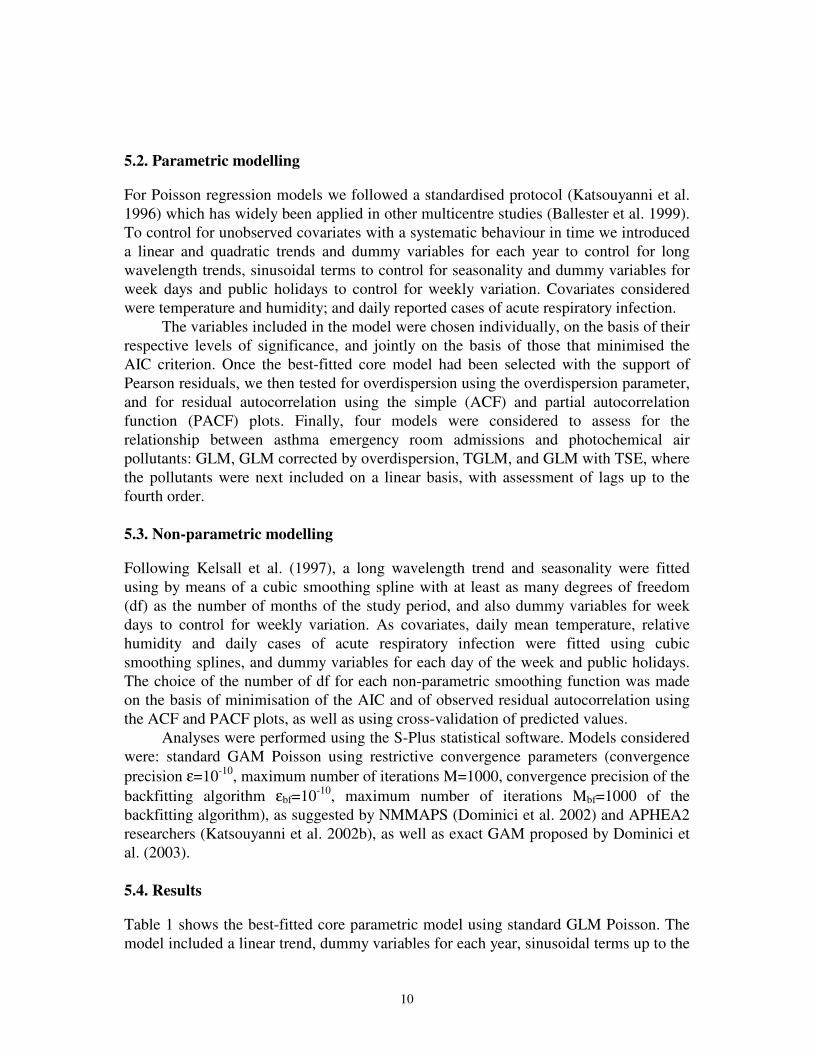
sixth order, dummy variables for each day of the week, also for public holidays (work
and school), linear and quadratic terms for temperature and humidity, and a linear term
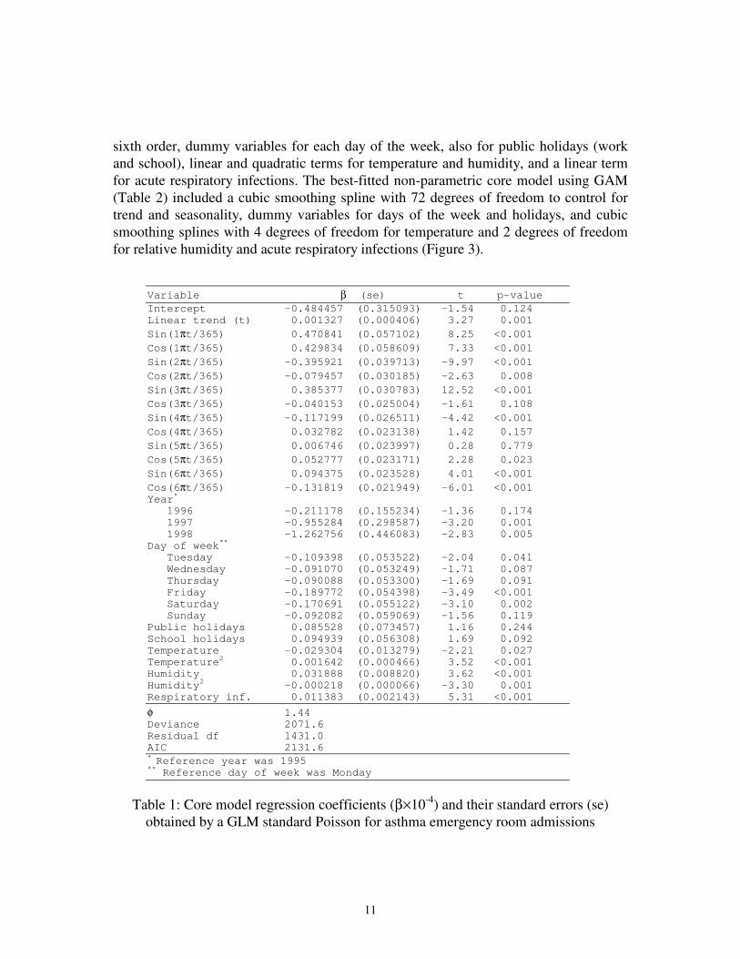
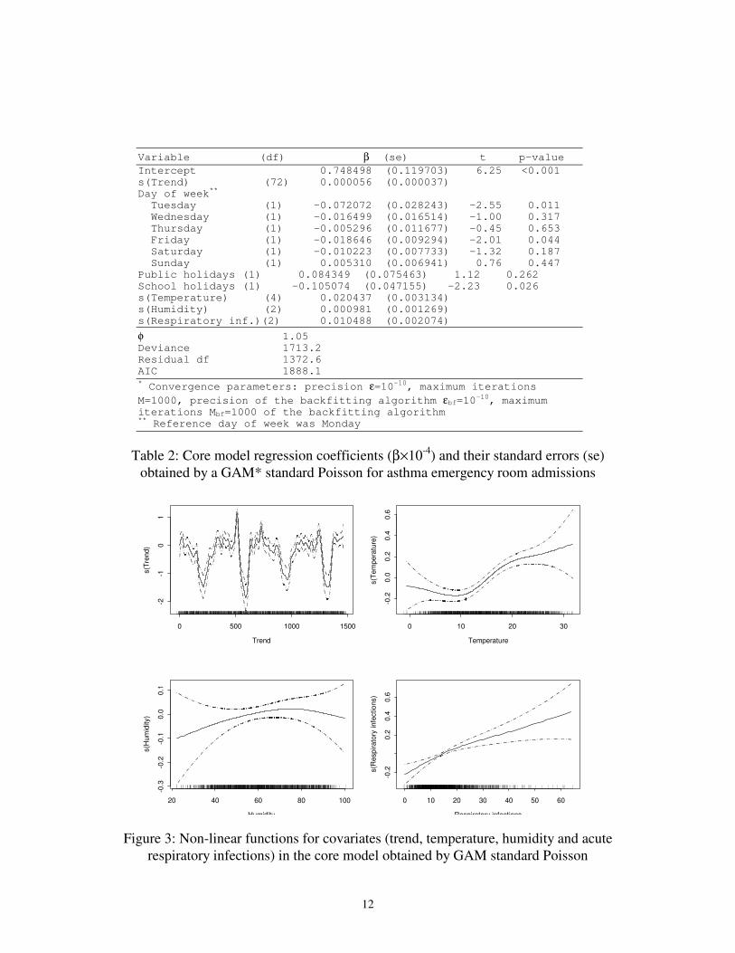
for acute respiratory infections. The best-fitted non-parametric core model using GAM
(Table 2) included a cubic smoothing spline with 72 degrees of freedom to control for
trend and seasonality, dummy variables for days of the week and holidays, and cubic
smoothing splines with 4 degrees of freedom for temperature and 2 degrees of freedom
for relative humidity and acute respiratory infections (Figure 3).
Variable β (se) t p-value
Intercept -0.484457 (0.315093) -1.54 0.124 Linear trend (t) 0.001327 (0.000406) 3.27 0.001
Sin(1πt/365) 0.470841 (0.057102) 8.25 <0.001
Cos(1πt/365) 0.429834 (0.058609) 7.33 <0.001
Sin(2πt/365) -0.395921 (0.039713) -9.97 <0.001
Cos(2πt/365) -0.079457 (0.030185) -2.63 0.008
Sin(3πt/365) 0.385377 (0.030783) 12.52 <0.001
Cos(3πt/365) -0.040153 (0.025004) -1.61 0.108
Sin(4πt/365) -0.117199 (0.026511) -4.42 <0.001
Cos(4πt/365) 0.032782 (0.023138) 1.42 0.157
Sin(5πt/365) 0.006746 (0.023997) 0.28 0.779
Cos(5πt/365) 0.052777 (0.023171) 2.28 0.023
Sin(6πt/365) 0.094375 (0.023528) 4.01 <0.001
Cos(6πt/365) -0.131819 (0.021949) -6.01 <0.001 Year
*
1996 -0.211178 (0.155234) -1.36 0.174 1997 -0.955284 (0.298587) -3.20 0.001 1998 -1.262756 (0.446083) -2.83 0.005 Day of week
**
Tuesday -0.109398 (0.053522) -2.04 0.041 Wednesday -0.091070 (0.053249) -1.71 0.087 Thursday -0.090088 (0.053300) -1.69 0.091 Friday -0.189772 (0.054398) -3.49 <0.001 Saturday -0.170691 (0.055122) -3.10 0.002 Sunday -0.092082 (0.059069) -1.56 0.119 Public holidays 0.085528 (0.073457) 1.16 0.244 School holidays 0.094939 (0.056308) 1.69 0.092 Temperature -0.029304 (0.013279) -2.21 0.027 Temperature
2 0.001642 (0.000466) 3.52 <0.001
Humidity 0.031888 (0.008820) 3.62 <0.001 Humidity
2 -0.000218 (0.000066) -3.30 0.001
Respiratory inf. 0.011383 (0.002143) 5.31 <0.001
φ 1.44 Deviance 2071.6 Residual df 1431.0 AIC 2131.6 * Reference year was 1995
** Reference day of week was Monday
Table 1: Core model regression coefficients (β×10-4
) and their standard errors (se)
obtained by a GLM standard Poisson for asthma emergency room admissions
12
Variable (df) β (se) t p-value
Intercept 0.748498 (0.119703) 6.25 <0.001 s(Trend) (72) 0.000056 (0.000037) Day of week
**
Tuesday (1) -0.072072 (0.028243) -2.55 0.011 Wednesday (1) -0.016499 (0.016514) -1.00 0.317 Thursday (1) -0.005296 (0.011677) -0.45 0.653 Friday (1) -0.018646 (0.009294) -2.01 0.044 Saturday (1) -0.010223 (0.007733) -1.32 0.187 Sunday (1) 0.005310 (0.006941) 0.76 0.447 Public holidays (1) 0.084349 (0.075463) 1.12 0.262 School holidays (1) -0.105074 (0.047155) -2.23 0.026 s(Temperature) (4) 0.020437 (0.003134) s(Humidity) (2) 0.000981 (0.001269) s(Respiratory inf.)(2) 0.010488 (0.002074)
φ 1.05 Deviance 1713.2 Residual df 1372.6 AIC 1888.1 * Convergence parameters: precision ε=10-10, maximum iterations
M=1000, precision of the backfitting algorithm εbf=10-10
, maximum iterations Mbf=1000 of the backfitting algorithm
** Reference day of week was Monday
Table 2: Core model regression coefficients (β×10-4
) and their standard errors (se)
obtained by a GAM* standard Poisson for asthma emergency room admissions
Trend
s(T
rend)
0 500 1000 1500
-2-1
01
Temperature
s(T
em
pera
ture
)
0 10 20 30
-0.2
0.0
0.2
0.4
0.6
Humidity
s(H
um
idity)
20 40 60 80 100
-0.3
-0.2
-0.1
0.0
0.1
Respiratory infections
s(R
espirato
ry infe
ctions)
0 10 20 30 40 50 60
-0.2
0.2
0.4
0.6
Figure 3: Non-linear functions for covariates (trend, temperature, humidity and acute
respiratory infections) in the core model obtained by GAM standard Poisson
13
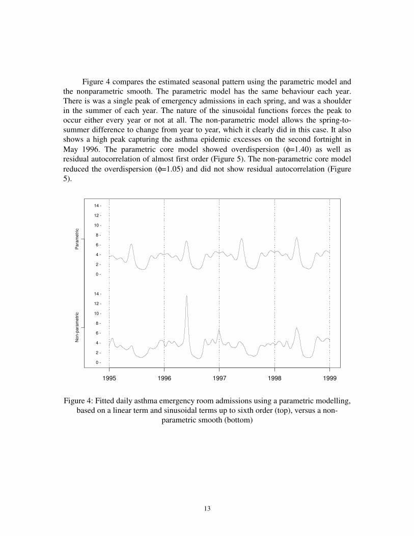
Figure 4 compares the estimated seasonal pattern using the parametric model and
the nonparametric smooth. The parametric model has the same behaviour each year.
There is was a single peak of emergency admissions in each spring, and was a shoulder
in the summer of each year. The nature of the sinusoidal functions forces the peak to
occur either every year or not at all. The non-parametric model allows the spring-to-
summer difference to change from year to year, which it clearly did in this case. It also
shows a high peak capturing the asthma epidemic excesses on the second fortnight in
May 1996. The parametric core model showed overdispersion (φ=1.40) as well as
residual autocorrelation of almost first order (Figure 5). The non-parametric core model
reduced the overdispersion (φ=1.05) and did not show residual autocorrelation (Figure
5).
1995 1996 1997 1998 1999
No
n-p
ara
me
tric
Pa
ram
etr
ic
0 -
2 -
4 -
6 -
8 -
10 -
12 -
14 -
0 -
2 -
4 -
6 -
8 -
10 -
12 -
14 -
Figure 4: Fitted daily asthma emergency room admissions using a parametric modelling,
based on a linear term and sinusoidal terms up to sixth order (top), versus a non-
parametric smooth (bottom)
14
ACF for GLM standard Poisson core model
Au
toco
rre
latio
n
Lag0 1 2 3 4 5 6 7 8 9 10
-.2
0
.2
.4
.6
.8
1
PACF for GLM standard Poisson core model
Pa
rtia
l a
uto
co
rre
latio
n
Lag0 1 2 3 4 5 6 7 8 9 10
-.2
-.1
0
.1
.2
ACF for GAM standard Poisson core model
Au
toco
rre
latio
n
Lag0 1 2 3 4 5 6 7 8 9 10
-.2
0
.2
.4
.6
.8
1
PACF for GAM standard Poisson core model
Pa
rtia
l a
uto
co
rre
latio
n
Lag0 1 2 3 4 5 6 7 8 9 10
-.2
-.1
0
.1
.2
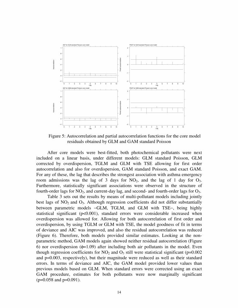
Figure 5: Autocorrelation and partial autocorrelation functions for the core model
residuals obtained by GLM and GAM standard Poisson
After core models were best-fitted, both photochemical pollutants were next
included on a linear basis, under different models: GLM standard Poisson, GLM
corrected by overdispersion, TGLM and GLM with TSE allowing for first order
autocorrelation and also for overdispersion, GAM standard Poisson, and exact GAM.
For any of these, the lag that describes the strongest association with asthma emergency
room admissions was the lag of 3 days for NO2, and the lag of 1 day for O3.
Furthermore, statistically significant associations were observed in the structure of
fourth-order lags for NO2, and current-day lag, and second- and fourth-order lags for O3.
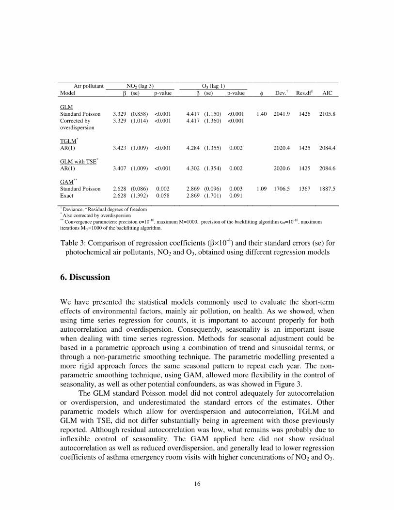
Table 3 sets out the results by means of multi-pollutant models including jointly
best lags of NO2 and O3. Although regression coefficients did not differ substantially
between parametric models −GLM, TGLM, and GLM with TSE−, being highly
statistical significant (p<0.001), standard errors were considerable increased when
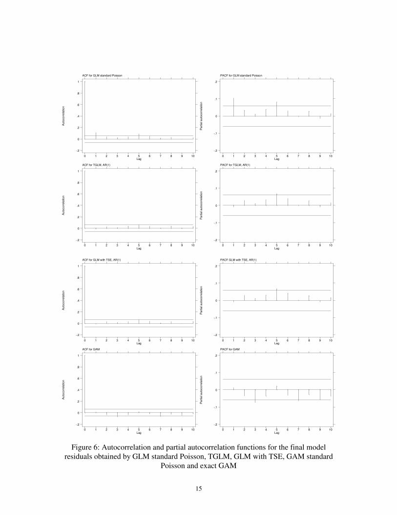
overdispersion was allowed for. Allowing for both autocorrelation of first order and
overdispersion, by using TGLM or GLM with TSE, the model goodness of fit in terms
of deviance and AIC was improved, and also the residual autocorrelation was reduced
(Figure 6). Therefore, both models provided similar estimates. Looking at the non-
parametric method, GAM models again showed neither residual autocorrelation (Figure
6) nor overdispersion (φ=1.09) after including both air pollutants in the model. Even
though regression coefficients for NO2 and O3 still were statistical significant (p=0.002
and p=0.003, respectively), but their magnitude were reduced as well as their standard
errors. In terms of deviance and AIC, the GAM model provided lower values than
previous models based on GLM. When standard errors were corrected using an exact
GAM procedure, estimates for both pollutants were now marginally significant
(p=0.058 and p=0.091).
15
ACF for GLM standard Poisson
Au
toco
rre
latio
n
Lag0 1 2 3 4 5 6 7 8 9 10
-.2
0
.2
.4
.6
.8
1
PACF for GLM standard Poisson
Pa
rtia
l a
uto
co
rre
latio
n
Lag0 1 2 3 4 5 6 7 8 9 10
-.2
-.1
0
.1
.2
ACF for TGLM, AR(1)
Au
toco
rre
latio
n
Lag0 1 2 3 4 5 6 7 8 9 10
-.2
0
.2
.4
.6
.8
1
PACF for TGLM, AR(1)
Pa
rtia
l a
uto
co
rre
latio
n
Lag0 1 2 3 4 5 6 7 8 9 10
-.2
-.1
0
.1
.2
ACF for GLM with TSE, AR(1)
Au
toco
rre
latio
n
Lag0 1 2 3 4 5 6 7 8 9 10
-.2
0
.2
.4
.6
.8
1
PACF GLM with TSE, AR(1)
Pa
rtia
l a
uto
co
rre
latio
n
Lag0 1 2 3 4 5 6 7 8 9 10
-.2
-.1
0
.1
.2
ACF for GAM
Au
toco
rre
latio
n
Lag0 1 2 3 4 5 6 7 8 9 10
-.2
0
.2
.4
.6
.8
1
PACF for GAM
Pa
rtia
l a
uto
co
rre
latio
n
Lag0 1 2 3 4 5 6 7 8 9 10
-.2
-.1
0
.1
.2
Figure 6: Autocorrelation and partial autocorrelation functions for the final model
residuals obtained by GLM standard Poisson, TGLM, GLM with TSE, GAM standard
Poisson and exact GAM
16
Air pollutant NO2 (lag 3) O3 (lag 1)
Model β (se) p-value β (se) p-value φ Dev.† Res.df‡ AIC
GLM
Standard Poisson
Corrected by
overdispersion
3.329
3.329
(0.858)
(1.014)
<0.001
<0.001
4.417
4.417
(1.150)
(1.360)
<0.001
<0.001
1.40
2041.9
1426
2105.8
TGLM*
AR(1)
3.423
(1.009)
<0.001
4.284
(1.355)
0.002
2020.4
1425
2084.4
GLM with TSE*
AR(1)
3.407
(1.009)
<0.001
4.302
(1.354)
0.002
2020.6
1425
2084.6
GAM**
Standard Poisson
Exact
2.628
2.628
(0.086)
(1.392)
0.002
0.058
2.869
2.869
(0.096)
(1.701)
0.003
0.091
1.09
1706.5
1367
1887.5
† Deviance, ‡ Residual degrees of freedom * Also corrected by overdispersion ** Convergence parameters: precision ε=10-10, maximum M=1000, precision of the backfitting algorithm εbf=10-10, maximum
iterations Mbf=1000 of the backfitting algorithm.
Table 3: Comparison of regression coefficients (β×10-4
) and their standard errors (se) for
photochemical air pollutants, NO2 and O3, obtained using different regression models
6. Discussion
We have presented the statistical models commonly used to evaluate the short-term
effects of environmental factors, mainly air pollution, on health. As we showed, when
using time series regression for counts, it is important to account properly for both
autocorrelation and overdispersion. Consequently, seasonality is an important issue
when dealing with time series regression. Methods for seasonal adjustment could be
based in a parametric approach using a combination of trend and sinusoidal terms, or
through a non-parametric smoothing technique. The parametric modelling presented a
more rigid approach forces the same seasonal pattern to repeat each year. The non-
parametric smoothing technique, using GAM, allowed more flexibility in the control of
seasonality, as well as other potential confounders, as was showed in Figure 3.
The GLM standard Poisson model did not control adequately for autocorrelation
or overdispersion, and underestimated the standard errors of the estimates. Other
parametric models which allow for overdispersion and autocorrelation, TGLM and
GLM with TSE, did not differ substantially being in agreement with those previously
reported. Although residual autocorrelation was low, what remains was probably due to
inflexible control of seasonality. The GAM applied here did not show residual
autocorrelation as well as reduced overdispersion, and generally lead to lower regression
coefficients of asthma emergency room visits with higher concentrations of NO2 and O3.
17
Standard errors were also reduced using GAM in comparison with those models which
control for seasonality using a parametric method. This fact has usually been justified by
the fact that the residual autocorrelation was removed by using a non-parametric
smoother of time. But when a GAM exact method was used, standard errors were
considerably increased, being closer to those provided by the parametric autoregressive
models, TGLM and GLM with TSE.
Alternative models, that we do not discuss further, have also been applied in the
analysis of epidemiological time series. Probably the most common choice has been the
Box-Jenkins methodology, through transfer function modelling (Box and Jenkins 1976).
This methodology has traditionally been used for forecasting applications in economics.
These models are very useful to describe changes over time, but the advantage of
regression methods in epidemiology over Box-Jenkins methodology is that regression
methods are more flexible. Box-Jenkins methods only can be applied to data with an
underlying normal structure. Box-Jenkins models are built with the aim of prediction
and use transformations in the dependent variables which turn the regression parameters
non-interpretable in an epidemiological manner. Moreover, the use of regression
methods enables the researcher to address for more specific hypotheses common to
epidemiology, such as dose-response curves, threshold models, interactions, cumulative
effects, or even effect modification. Also interpretation of the results from a regression
model for counts is more familiar and straightforward for the epidemiologist in terms of
relative risks. However, Box-Jenkins models have also been applied in air pollution
(Diaz et al. 1999) and temperature studies (Saez et al. 1995). It has also been showed
that it results did not differ from regression methods when the health outcome is non-
normally distributed, like hospital or emergency room admissions (Tobías et al. 2001).
Independently of the statistical model used, there are different interpretations of
time series when the outcome is mortality or something like admissions to hospital
which can occur more than once. The fundamental difficulty is that the analysis can only
examine short term effects. Let us imagine a data set in which deaths or hospital
admissions were evenly spread throughout the week, and also suppose that through a
clerical error, deaths which occurred before midday on Saturday were included in
Friday’s total. Then Friday would have 50% more deaths than the average, and Saturday
50% less. In any time series regression model, the risk for Friday would appear as 1.5,
and is likely to be highly significant. However, the overall death rate is unaffected. In air
pollution studies, it may be that the air pollution hastens deaths or hospital admissions
in susceptible individuals by one day. This is known as harvesting (Zeger et al. 1999,
Schwartz 2000). So, although the risk is high, the effect in terms of person-years lost in
the community is likely to be very low. Thus it is important to appreciate that a
significant risk is not necessarily an important one from a public health view point. To
examine long term effects one has to compare communities which are standardised for
the main risk factors such as age, sex and race, but have different levels of pollution
(Kunzli et al. 2001). Of course, historical levels of pollution also need to be considered,
because it is likely that it will have effect which may take years to become evident.
18
Another difficulty is that the effect may take several days to build up. If deaths
occur in the early evening, they may be attributed to the following day. Thus one should
examine lagged effects of the pollutant. This means that the risk of a particular pollutant
should be attributable to a particular day. It can be difficult to compare cities if the lag
structure of the models is different (Samet et al. 2000, Katsouyanni et al. 2002). A
further problem is in separating out the effects of different pollutants. Most are very
highly correlated, and it is very difficult to disentangle which are the important ones.
Statistical solutions are usually somewhat of a compromise. However, this is a highly
political area, because different pollutants have different sources, such as from cars,
lorries or industry, and blaming one pollutant at the expense of the others requires very
strong evidence from the data, and this is usually lacking.
We have showed that different models lead to different estimates. Care is needed
in their interpretation, and careful reporting so it is clear how variables have been
modelled. In this context, GAM presents the best model fit in terms of absence of
autocorrelation and reduction of overdispersion, leading to more efficient estimates.
Moreover, GAM can be useful to suggests functional forms for the parametric
modelling, or for checking an existing parametric model for bias. Thus, we venture to
suggest the use of GAM methods in the modelling of epidemiological time series.
References
Akaike, H. (1973), Information theory and an extension of the maximum
likelihood principal, in Petrov, B. N. and Csaki, F. (Eds.) Second International
Symposium on Information Theory, Akademia Kiao, Budapest.
Ballester, F., Saez, M., Alonso, M. E., Taracido, M., Ordonez, J. M., Aguinaga, I.
and The EMECAM project: the Spanish multicenter study on the relationship between
air pollution and mortality (1999), The background, participants, objectives and
methodology, Revista Española de Salud Publica, 73, 165-175.
Braga, A.L., Zanobetti, A. and Schwartz J (2001), The time course of weather-
related deaths, Epidemiology, 12, 662-667.
Box, G. E. P. and Jenkins, G. M. (1976), Time series Analysis, Holden-Day, San
Francisco; Holden-Day.
Brumback, B. A., Ryan, L. M., Schwartz, J. D., Neas, L. M., Stark, P. C. and
Burge, H. A. (2000), Transitional regression models, with application to environmental
time series, Journal of the American Statistical Association, 95, 16-27.
Campbell, M. J. (1994), Time series regression for counts: an investigation into
the relationship between Sudden Infant Death Syndrome and environmental
temperature, Journal of the Royal Statistical Society, Series A, 157, 191-208.
Campbell, M. J. (1998), Time series regression, in Armitage, P. and Colton, T.
(Eds.), Encyclopaedia of Biostatistics, New York, Wiley (pp. 4936-4938).
19
Campbell, M. J., Julious, S. A., Peterson, C. K. and Tobias, A. (2001),
Atmospheric pressure and sudden infant death syndrome in Cook County, Chicago,
Paediatric and Perinatal Epidemiology, 15, 287-289.
Chambers, J. and Hastie, T. (1992), Statistical Models in S. London, Chapman and
Hall.
Diaz, J., Garcia, R., Ribera, P., Alberdi, J.C., Hernández, E., Pajares, M. S., Otero,
A. (1999), Modelling of air pollution and its relationship with mortality and morbidity
in Madrid, Spain, International Archieves of Occupational and Environmental Health,
72, 366-376.
Dominici, F., McDermott, A., Zeger, S.L. and Samet, J.M. (2002), On
Generalized Additive Models in time series studies of air pollution and health, American
Journal of Epidemiology, 156, 1-11.
Dominici, F., McDermott, A. and Hastie, T. (2003), Issues in semi-parametric
regression with applications in time series regression models for air pollution and
mortality, Available at http://www.ihapss.jhsph.edu/
Fitmaurice, G. M. (1998), Regression models for discrete longitudinal data, in
Everitt, B. S. and Dunn, G. (Eds.), Statistical Analysis of Medical Data, London,
Arnold.
Galán, I., Tobías, A., Banegas, J. R. and Aranguez, E. (2003), Short-term effects
of air pollution on daily asthma emergency room admissions in Madrid, Spain.
European Respiratory Journal, 22: 802-808.
Green, P. J. and Silverman, B. W. (1994), Nonparametric Regression and
Generalized Linear Models, London, Chapman and Hall.
Hastie, T. J. and Tibshirani, R. J. (1990), Generalized Additive Models, London,
Chapman and Hall.
Hatzakis, A., Katsouyanni, K., Kalandidi, A., Day, N. and Trichopoulos, D.
(1986), Short-term effects of air pollution on mortality in Athens, International Journal
of Epidemiology, 15, 73-81.
Katsouyanni, K., Schwartz, J., Spix, C., Touloumi, G., Zmirou, D. and Zanobetti,
A. (1996), Short term effects of air pollution on health: a European approach using
epidemiologic time series data: the APHEA protocol, Journal of Epidemiology and
Community Health, 50 (Suppl.1), S12-S18.
Katsouyanni, K., Touloumi, G., Samoli, E., Gryparis, A., Le Tertre, A.,
Monopolis, Y. and Rossi, G. (2002), Confounding and effect modification in the short-
term effects of ambient particles on total mortality: results from 29 European cities
within the APHEA 2 project, Epidemiology, 12, 521-531.
Katsouyanni, K., Toloumi, G., Samoli, E., Gryparis, A., Manopolis, Y., and Le
Tertre, A. (2002b), Different convergence parameters applied to the S-Plus gam
function, Epidemiology, 13, 742.
Kelsall, J. E., Samet, J. M., Zeger, S. L. and Xu, J. (1997), Air pollution and
mortality in Philadelphia, 1974-1988, American Journal of Epidemiology, 146, 750-762.
Kunzli, N., Medina, S., Kaiser, R., Quenel, P., Horak, F. Jr. and Studnicka, M.
(2001), Assessment of deaths attributable to air pollution: should we use risk estimates
20
based on time series or on cohort studies?. American Journal of Epidemiology, 153,
1050-1055.
McCullagh P. and Nelder J. (1989), Generalised Linear Models, London,
Chapman and Hall.
Mackenbach, J. P., Knust, A. E. and Looman, C. W. N. (1992), Seasonal variation
in mortality in the Netherlands, Journal of Epidemiology and Community Health, 46,
261-265.
Ramsay, T., Burnett, R. and Krewski D. (2003), The effect of concurvity in
generalized additive models linking mortality and ambient air pollution, Epidemiology,
14, 18-23.
Saez, M., Sunyer, J., Castellsagué, J. and Antó J. M. (1995), Relation between
temperature and mortality, International Journal of Epidemiology, 24, 576-582.
Samet, J. M., Zeger, S. L., Dominici, F., Curriero, F., Coursac, I. and Dockery, D.
W. (2000), The National Morbidity, Mortality, and Air Pollution Study. Part II:
Morbidity and mortality from air pollution in the United States, Research Report of the
Health Effects Institute, 94 (Pt 2), 5-70.
Schwartz, J. (1994), Non-parametric smoothing in the analysis of air pollution and
respiratory illness, Canadian Journal of Statistics, 4, 471-487.
Schwartz, J., Spix, C., Touloumi, G., Bacharova, L., Barumamdzadeh, T. and le
Terte, A. (1996), Methodological issues in studies of air pollution and daily counts of
deaths or hospital admissions, Journal of Epidemiology and Community Health, 50
(Suppl. 1) S3-S11.
Schwartz, J., Levin, R. and Hodge, K. (1997), Drinking water turbidity and
paediatric hospital use for gastrointestinal illness in Philadelphia, Epidemiology, 8, 615-
620.
Schwartz, J. (2000), Harvesting and long term exposure effects in the relation
between air pollution and mortality, American Journal of Epidemiology, 151, 440-448.
Staneck, E. J., Shetterley, S. S., Allen, L. H., Pelto, G. H. and Chavez A. (1989),
A cautionary note on the use of autoregressive models in analysis of longitudinal data.
Statistics in Medicine, 8, 1523-1528.
Tobías, A., Díaz, J., Sáez, M. and Alberdi, J. C. (2001), Use of Poisson regression
and Box-Jenkins models to evaluate the short-term effects of environmental noise levels
on daily emergency admissions in Madrid, Spain, European Journal of Epidemiology,
17, 765-771.
Touloumi, G., Atkinson, R., Le Tertre, A., Samoli, E., Schwartz, J., Schlinder, C.,
Vonk, J. M., Rossi, G., Saez, M., Rabszenko, D. and Katsouyanni, K. (2003), Analysis
of health outcome time series data in epidemiological studies. Environmetrics (in
press).
Wahba, G. (1990), Spline Functions for Observational Data. Philadelphia,
CBMS-NSF Regional Conference Series, SIAM.
Yule, G. U. (1926), Why do we sometimes get nonsense-correlations between
time series?. A study in sampling and the nature of time series, Journal of the Royal
Statistical Society, 89, 187-227.

21
Zeger, S.L., Dominici, F. and Samet, J. (1999), Harvesting-resistant estimates of
air pollution effects on mortality, Epidemiology, 10, 171-175.