Embed Size (px)
Citation preview
Mathematical Theory and Modeling www.iiste.org
ISSN 2224-5804 (Paper) ISSN 2225-0522 (Online)
Vol.4, No.8, 2014
29
Time Series Forecasting of Solid Waste Generation in Arusha City
- Tanzania
Amon Mwenda1*
, Dmitry Kuznetsov1, Silas Mirau
1
1. School of Mathematics, Computational and Communication Science and Engineering, Nelson
Mandela Institution of Science and Technology (NM-AIST), P.O. Box 447, Arusha, Tanzania
*E-mail of the corresponding author: [email protected]
Abstract
Statistical time series modeling is widely used in prediction and forecasting studies. This study intends to
analyze, compare and select the best time series model for forecasting amount of solid waste generation for the
next years in Arusha city - Tanzania among ARMA/ARIMA and Exponential Smoothing models. The past data
used are monthly amount of solid waste collected by the city authorities from year 2008 to 2013. The result
indicated that ARIMA (1, 1, 1) outperformed other potential models in terms of MAPE, MAD and RMSE
measures and hence used to forecast the amount of the solid waste generation for the next years.
Keywords: ARIMA models, Exponential Smoothing models, time series, MAPE, MAD, RMSE
1. Introduction
Solid waste are materials of all sorts regarded as useless and are disposed. In urban areas there are disposal
points in various locations for people to dispose. In African cities poor management of solid waste is a common
phenomenon due to budgetary problems, mismatching plans and inadequate information about the amount of
solid waste generated by residents (Simelane and Mohee, 2012). Forecasting of solid waste generation rate is
therefore important to city authorities to help them in the policy making and proper planning of operations
related to solid waste management. Arusha city in Tanzania is one of the cities facing the problem of inefficient
collection and disposal of solid waste. Population is among the major factors contributing to high amount of
solid waste generation. Arusha city has a population of about 416,442 with an average annual increase rate of
about 2.7% (NBS, 2013). With this population, if no proper measures taken to improve its management relative
to the increasing population, consequences are bad. Furthermore, there are no published figures of solid waste
generation and their trend in Tanzanian cities. The effect of uncollected solid waste include possible diseases
outbreak and also blocks the city drainage systems bringing rise to other problems. This fact motivated this study
of forecasting solid waste generation in the next five years so that Arusha city authorities can have useful
information about the dynamics of solid waste generation to aid in their planning and operations.
The selection of a technique to forecast a subject depend on many factors – the accuracy desired, the context of
forecast, the relevance and availability of statistical data, the time period to be forecast, the cost/benefit of the
forecast, easiness of interpretation, guidelines from the literature and implementation (Armstrong, J. S., 2011). In
this study, statistical modeling techniques ARIMA and Exponential smoothing are used. Ebenezer et al (2013)
analyzed ARIMA models in forecasting Kumasi Metropolitan Area solid waste generation and obtained
substantial results which were useful to the KMA authority. In their study, ARIMA (1, 1, 1) was selected as the best
model. A study on application and evaluation of forecasting methods for municipal solid waste generation
conducted in Kaunas – Lithuania in Eastern Europe exposed difficult in forecasting of municipal solid waste
generation due to lack of data and selection of methods for the available data. The study implemented regression
analysis for social – economic indicators of solid waste generation and time series analysis. Time series forecasting
were found to be most accurate for forecasting short interval variation and results were useful to decision – makers
in developing countries (Ingrida, R., et al, 2012).
2 Statistical Model
Time series analysis goes through specified set of procedures and the results at one stage is a decisive factor on
what to do in the next stage. This study used a popular Box – Jenkins approach. This approach involves about
four stages before real forecasting namely stationarity checking, model identification, parameter estimation and
diagnostic checking. The approach use historical data as it input to generate future values. The models’ work
under assumptions that the data available are mean and variance stationary and the random errors or the
difference between observed and forecasted values are uncorrelated. See Box and Jenkins (1976), Brockwell and
Mathematical Theory and Modeling www.iiste.org
ISSN 2224-5804 (Paper) ISSN 2225-0522 (Online)
Vol.4, No.8, 2014
30
Davis (2002), Montgomery, Jennings and Kulahci (2008), Chatfield (2000) for details of these steps.
Most real life time series are stochastic. A stochastic time series is stationary if its statistical properties such as
mean and variance do not change over time. Plots of the original data, autocorrelation (ACF) and partial
autocorrelation (PACF) are examined for trend, seasonal components, cyclic and outliers. If these patterns are
observed they can be removed by differencing the series to obtain stationary residuals (Brockwell & Davis,
2002). An alternative for stationarity checking is the Dickey – Fuller unit root test. This determines if a time
series needs differencing or not (Stevenson, 2003).
When time series has achieved stationarity, model identification is done by examining the ACF and PACF plots.
The order are identified by matching the patterns of ACF and PACF plots. When ACF decays quickly then spikes
observed in PACF gives the AR order and when PACF decays quickly, ACF‘s significant lags give the order of
MA terms. When both ACF and PACF plots decays mixed model is considered. Parameters of the identified
models are estimated by method of maximum likelihood, moments or the method of least square (Brockwell and
Davis, 2002).
Diagnostic checking involves checking if the estimated parameters adequately fit the data. Examination of
residual autocorrelation is one such method in which the plots of ACF and PACF residuals are checked for white
noise properties. If the model sufficiently fit the data, the autocorrelation of the residual should not be
significantly different from zero for lags greater than one. Another approach in checking adequacy of the fitted
model is by computing Ljung – Box statistic.
When the observed time series are stationary and need no differencing, the ARMA (p, q) is fitted. The general
equation of ARMA (p, q) is:
(1 − 𝜙1𝐵−. . . −𝜙𝑝𝐵𝑝)𝑋𝑡 = (1 − 𝜃1𝐵−. . . −𝜃𝑞𝐵𝑞)𝑎𝑡
Where p and q are the orders of autoregressive and moving average components respectively, B is the backshift
operator, 𝑋𝑡 is the quantity predicted at time t, 𝜙𝑝 and 𝜃𝑞 are parameters.
When the observed data needs differencing to achieve stationarity, the ARIMA (p, d, q) is fitted. The general
equation for ARIMA (p, d, q) is:
(1 − 𝜙1𝐵−. . . −𝜙𝑝𝐵𝑝)(1 − 𝐵)𝑑𝑋𝑡 = (1 − 𝜃1𝐵−. . . −𝜃𝑞𝐵𝑞)𝑎𝑡
Where d is the order of differencing.
Exponential smoothing models existing in the literature are Simple/single Exponential Smoothing (SES), Double
Exponential (Holt) Smoothing (DES)/Linear Exponential Smoothing and Triple Exponential Smoothing (TES).
Simple exponential smoothing is for series which are stationary, double exponential smoothing are for series
which exhibit trend and triple exponential smoothing is for series with trend and seasonality. The general
equations for the three models are shown next (Mentzer, 2005).
Simple Exponential Smoothing (SES) has one smoothing equation with one parameter:
𝐹𝑡+1 = 𝛼𝑋𝑡 + (1 − 𝛼)𝐹𝑡−1
Double exponential smoothing (DES) has two smoothing equations with two parameters:
𝐿𝑡 = 𝛼𝑋𝑡 + (1 − 𝛼)(𝐿𝑡−1 + 𝑇𝑡−1)
𝑇𝑡 = 𝛾(𝐿𝑡 − 𝐿𝑡−1) + (1 − 𝛾)𝑇𝑡−1
𝐹𝑡+𝑝 = 𝐿𝑡 + 𝑝𝑇𝑡
Triple exponential smoothing has three smoothing equations with three parameters:
𝐿𝑡 = 𝛼𝑋𝑡 + (1 − 𝛼)(𝐿𝑡−1 + 𝑇𝑡−1)
𝑇𝑡 = 𝛾(𝐿𝑡 − 𝐿𝑡−1) + (1 − 𝛾)𝑇𝑡−1
𝑆𝑡 = 𝛿(𝑋𝑡 − 𝐿𝑡) + (1 − 𝛿)𝑆𝑡−1
𝐹𝑡+𝑝 = 𝐿𝑡 + 𝑝𝑇𝑡 + 𝑆𝑡+𝑝−𝑙
Where 𝐿𝑡 = current level, 𝑇𝑡 = current trend level 𝑆𝑡 = Current seasonality level
𝐹𝑡+𝑝 = Forecast after period 𝑝, and 𝛼, 𝛾, 𝛿 = smoothing parameters
Various fit and performance criteria are used to choose the best forecasting model. These performance criteria
include Mean Absolute Percentage Error (MAPE), Mean Absolute Deviation (MAD), Root Mean Squared Error
(RMSE), R – square, Akaike Information criterion (AIC) and Schwarz Bayesian Information Criterion (SBIC).
Mathematical Theory and Modeling www.iiste.org
ISSN 2224-5804 (Paper) ISSN 2225-0522 (Online)
Vol.4, No.8, 2014
31
3. Results and discussion
Data used in this study were records of monthly amount of solid waste collected for disposal from Arusha City
by health department of the city council from July 2008 to December 2013. A total of 66 observations are
available, of which 60 are used for model formulation and 6 hold of for model validation.
3.1 Stationarity test
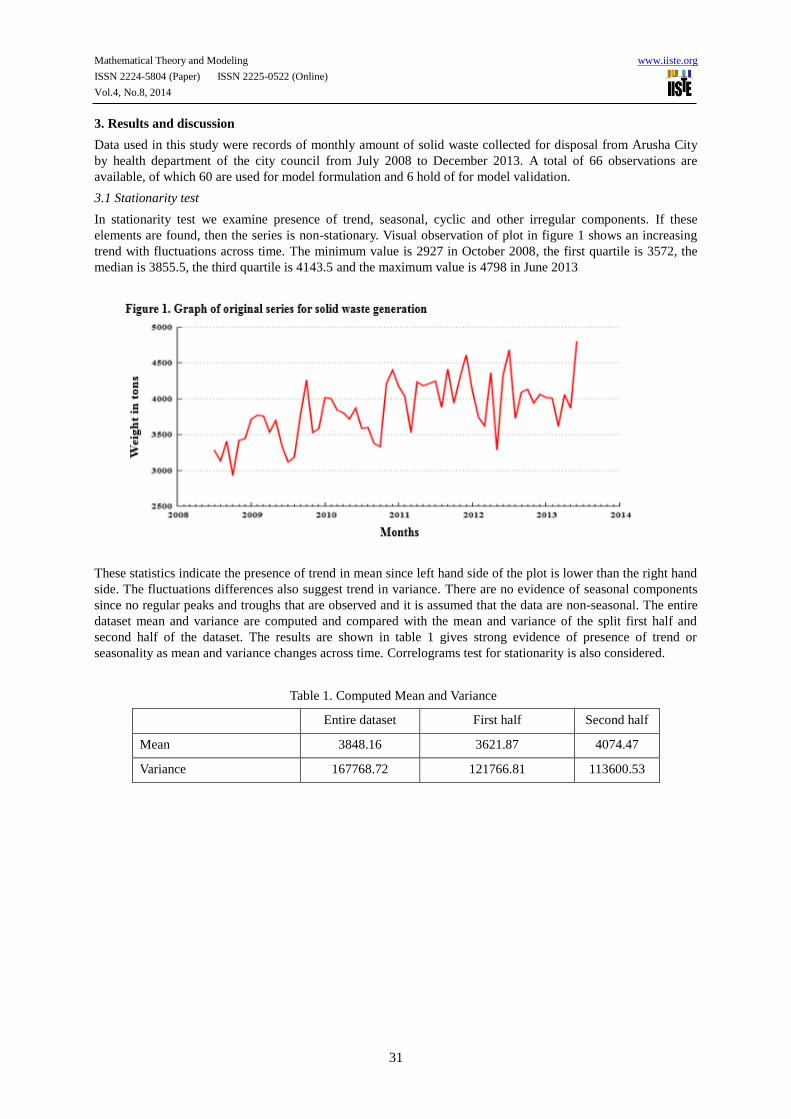
In stationarity test we examine presence of trend, seasonal, cyclic and other irregular components. If these
elements are found, then the series is non-stationary. Visual observation of plot in figure 1 shows an increasing
trend with fluctuations across time. The minimum value is 2927 in October 2008, the first quartile is 3572, the
median is 3855.5, the third quartile is 4143.5 and the maximum value is 4798 in June 2013
These statistics indicate the presence of trend in mean since left hand side of the plot is lower than the right hand
side. The fluctuations differences also suggest trend in variance. There are no evidence of seasonal components
since no regular peaks and troughs that are observed and it is assumed that the data are non-seasonal. The entire
dataset mean and variance are computed and compared with the mean and variance of the split first half and
second half of the dataset. The results are shown in table 1 gives strong evidence of presence of trend or
seasonality as mean and variance changes across time. Correlograms test for stationarity is also considered.
Table 1. Computed Mean and Variance
Entire dataset First half Second half
Mean 3848.16 3621.87 4074.47
Variance 167768.72 121766.81 113600.53
Mathematical Theory and Modeling www.iiste.org
ISSN 2224-5804 (Paper) ISSN 2225-0522 (Online)
Vol.4, No.8, 2014
32
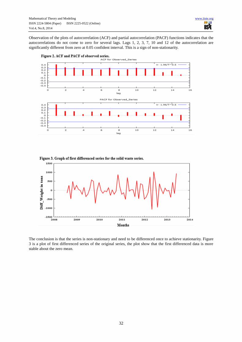
Observation of the plots of autocorrelation (ACF) and partial autocorrelation (PACF) functions indicates that the
autocorrelations do not come to zero for several lags. Lags 1, 2, 3, 7, 10 and 12 of the autocorrelation are
significantly different from zero at 0.05 confident interval. This is a sign of non-stationarity.
The conclusion is that the series is non-stationary and need to be differenced once to achieve stationarity. Figure
3 is a plot of first differenced series of the original series, the plot show that the first differenced data is more
stable about the zero mean.
Mathematical Theory and Modeling www.iiste.org
ISSN 2224-5804 (Paper) ISSN 2225-0522 (Online)
Vol.4, No.8, 2014
33
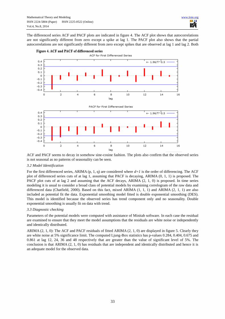
The differenced series ACF and PACF plots are indicated in figure 4. The ACF plot shows that autocorrelations
are not significantly different from zero except a spike at lag 1. The PACF plot also shows that the partial
autocorrelations are not significantly different from zero except spikes that are observed at lag 1 and lag 2. Both
ACF and PACF seems to decay in somehow sine-cosine fashion. The plots also confirm that the observed series
is not seasonal as no patterns of seasonality can be seen.
3.2 Model Identification
For the first differenced series, ARIMA (p, 1, q) are considered where d=1 is the order of differencing. The ACF
plot of differenced series cuts of at lag 1, assuming that PACF is decaying, ARIMA (0, 1, 1) is proposed. The
PACF plot cuts of at lag 2 and assuming that the ACF decays, ARIMA (2, 1, 0) is proposed. In time series
modeling it is usual to consider a broad class of potential models by examining correlogram of the raw data and
differenced data (Chatfield, 2000). Based on this fact, mixed ARIMA (1, 1, 1) and ARIMA (2, 1, 1) are also
included as potential fit the data. Exponential smoothing model fitted is double exponential smoothing (DES).
This model is identified because the observed series has trend component only and no seasonality. Double
exponential smoothing is usually fit on data with trend.
3.3 Diagnostic checking
Parameters of the potential models were computed with assistance of Minitab software. In each case the residual
are examined to ensure that they meet the model assumptions that the residuals are white noise or independently
and identically distributed.
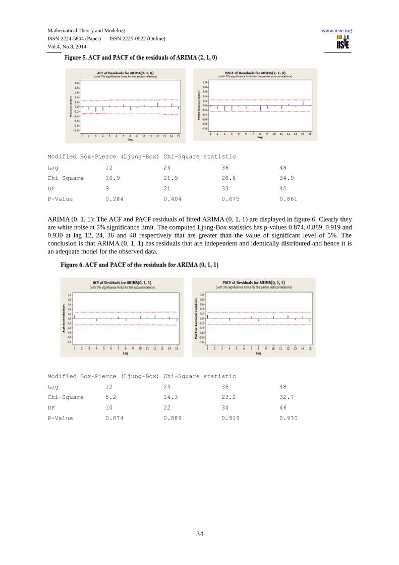
ARIMA (2, 1, 0): The ACF and PACF residuals of fitted ARIMA (2, 1, 0) are displayed in figure 5. Clearly they
are white noise at 5% significance limit. The computed Ljung-Box statistics has p-values 0.284, 0.404, 0.675 and
0.861 at lag 12, 24, 36 and 48 respectively that are greater than the value of significant level of 5%. The
conclusion is that ARIMA (2, 1, 0) has residuals that are independent and identically distributed and hence it is
an adequate model for the observed data.
Mathematical Theory and Modeling www.iiste.org
ISSN 2224-5804 (Paper) ISSN 2225-0522 (Online)
Vol.4, No.8, 2014
34
Modified Box-Pierce (Ljung-Box) Chi-Square statistic
Lag 12 24 36 48
Chi-Square 10.9 21.9 28.8 34.9
DF 9 21 33 45
P-Value 0.284 0.404 0.675 0.861
ARIMA (0, 1, 1): The ACF and PACF residuals of fitted ARIMA (0, 1, 1) are displayed in figure 6. Clearly they
are white noise at 5% significance limit. The computed Ljung-Box statistics has p-values 0.874, 0.889, 0.919 and
0.930 at lag 12, 24, 36 and 48 respectively that are greater than the value of significant level of 5%. The
conclusion is that ARIMA (0, 1, 1) has residuals that are independent and identically distributed and hence it is
an adequate model for the observed data.
Modified Box-Pierce (Ljung-Box) Chi-Square statistic
Lag 12 24 36 48
Chi-Square 5.2 14.3 23.2 32.7
DF 10 22 34 46
P-Value 0.874 0.889 0.919 0.930
Mathematical Theory and Modeling www.iiste.org
ISSN 2224-5804 (Paper) ISSN 2225-0522 (Online)
Vol.4, No.8, 2014
35
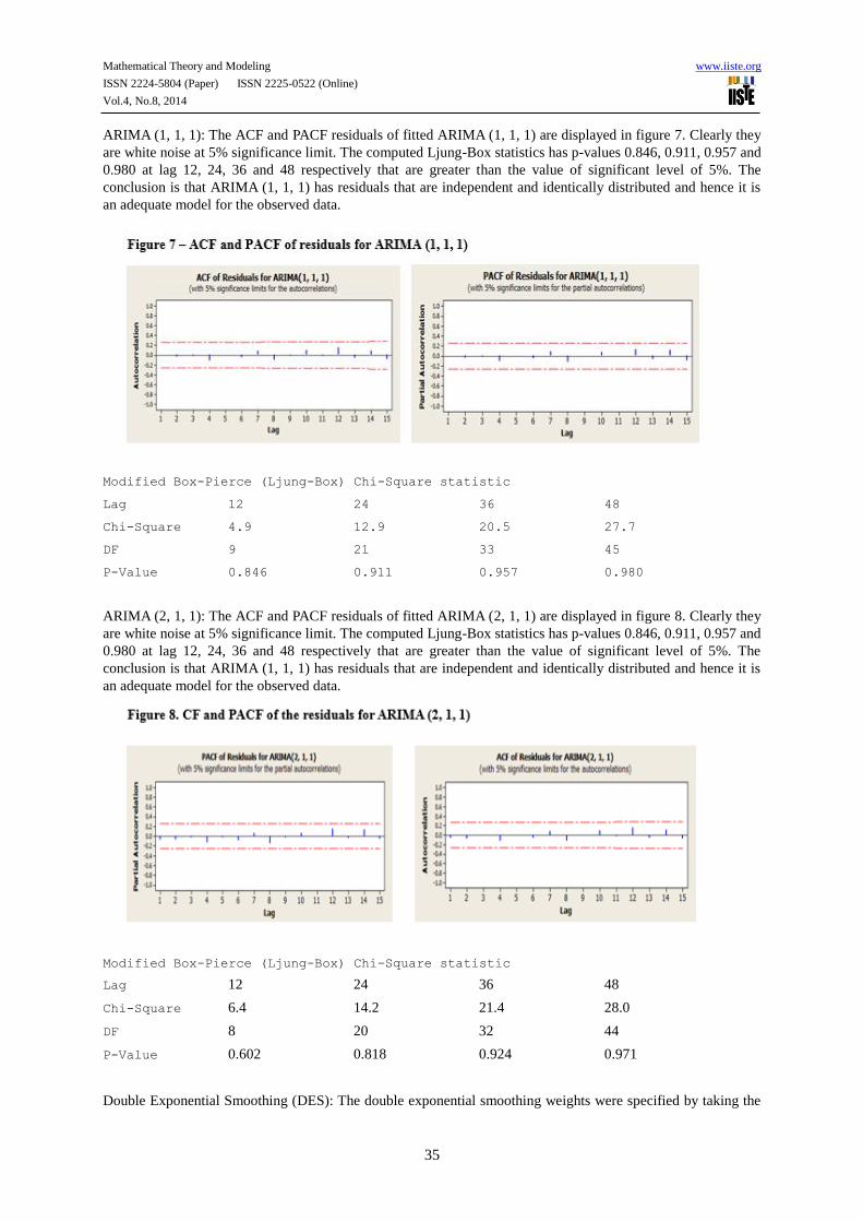
ARIMA (1, 1, 1): The ACF and PACF residuals of fitted ARIMA (1, 1, 1) are displayed in figure 7. Clearly they
are white noise at 5% significance limit. The computed Ljung-Box statistics has p-values 0.846, 0.911, 0.957 and
0.980 at lag 12, 24, 36 and 48 respectively that are greater than the value of significant level of 5%. The
conclusion is that ARIMA (1, 1, 1) has residuals that are independent and identically distributed and hence it is
an adequate model for the observed data.
Modified Box-Pierce (Ljung-Box) Chi-Square statistic
Lag 12 24 36 48
Chi-Square 4.9 12.9 20.5 27.7
DF 9 21 33 45
P-Value 0.846 0.911 0.957 0.980
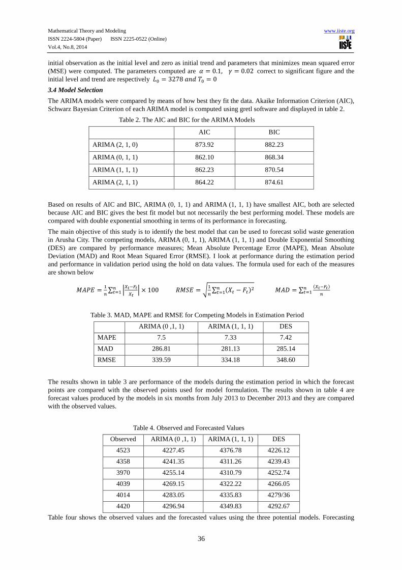
ARIMA (2, 1, 1): The ACF and PACF residuals of fitted ARIMA (2, 1, 1) are displayed in figure 8. Clearly they
are white noise at 5% significance limit. The computed Ljung-Box statistics has p-values 0.846, 0.911, 0.957 and
0.980 at lag 12, 24, 36 and 48 respectively that are greater than the value of significant level of 5%. The
conclusion is that ARIMA (1, 1, 1) has residuals that are independent and identically distributed and hence it is
an adequate model for the observed data.
Modified Box-Pierce (Ljung-Box) Chi-Square statistic
Lag 12 24 36 48
Chi-Square 6.4 14.2 21.4 28.0
DF 8 20 32 44
P-Value 0.602 0.818 0.924 0.971
Double Exponential Smoothing (DES): The double exponential smoothing weights were specified by taking the
Mathematical Theory and Modeling www.iiste.org
ISSN 2224-5804 (Paper) ISSN 2225-0522 (Online)
Vol.4, No.8, 2014
36
initial observation as the initial level and zero as initial trend and parameters that minimizes mean squared error
(MSE) were computed. The parameters computed are 𝛼 = 0.1, 𝛾 = 0.02 correct to significant figure and the
initial level and trend are respectively 𝐿0 = 3278 𝑎𝑛𝑑 𝑇0 = 0
3.4 Model Selection
The ARIMA models were compared by means of how best they fit the data. Akaike Information Criterion (AIC),
Schwarz Bayesian Criterion of each ARIMA model is computed using gretl software and displayed in table 2.
Table 2. The AIC and BIC for the ARIMA Models
AIC BIC
ARIMA (2, 1, 0) 873.92 882.23
ARIMA (0, 1, 1) 862.10 868.34
ARIMA (1, 1, 1) 862.23 870.54
ARIMA (2, 1, 1) 864.22 874.61
Based on results of AIC and BIC, ARIMA (0, 1, 1) and ARIMA (1, 1, 1) have smallest AIC, both are selected
because AIC and BIC gives the best fit model but not necessarily the best performing model. These models are
compared with double exponential smoothing in terms of its performance in forecasting.
The main objective of this study is to identify the best model that can be used to forecast solid waste generation
in Arusha City. The competing models, ARIMA (0, 1, 1), ARIMA (1, 1, 1) and Double Exponential Smoothing
(DES) are compared by performance measures; Mean Absolute Percentage Error (MAPE), Mean Absolute
Deviation (MAD) and Root Mean Squared Error (RMSE). I look at performance during the estimation period
and performance in validation period using the hold on data values. The formula used for each of the measures
are shown below
𝑀𝐴𝑃𝐸 =1
𝑛∑ |
𝑋𝑡−𝐹𝑡
𝑋𝑡| × 100𝑛
𝑡=1 𝑅𝑀𝑆𝐸 = √1
𝑛∑ (𝑋𝑡 − 𝐹𝑡)2𝑛
𝑡=1 𝑀𝐴𝐷 = ∑(𝑋𝑡−𝐹𝑡)
𝑛
𝑛𝑡=1
Table 3. MAD, MAPE and RMSE for Competing Models in Estimation Period
ARIMA (0 ,1, 1) ARIMA (1, 1, 1) DES
MAPE 7.5 7.33 7.42
MAD 286.81 281.13 285.14
RMSE 339.59 334.18 348.60
The results shown in table 3 are performance of the models during the estimation period in which the forecast
points are compared with the observed points used for model formulation. The results shown in table 4 are
forecast values produced by the models in six months from July 2013 to December 2013 and they are compared
with the observed values.
Table 4. Observed and Forecasted Values
Observed ARIMA (0 ,1, 1) ARIMA (1, 1, 1) DES
4523 4227.45 4376.78 4226.12
4358 4241.35 4311.26 4239.43
3970 4255.14 4310.79 4252.74
4039 4269.15 4322.22 4266.05
4014 4283.05 4335.83 4279/36
4420 4296.94 4349.83 4292.67
Table four shows the observed values and the forecasted values using the three potential models. Forecasting
Mathematical Theory and Modeling www.iiste.org
ISSN 2224-5804 (Paper) ISSN 2225-0522 (Online)
Vol.4, No.8, 2014
37
performance is computed for each case. The computed MAD, MAPE and RMSE from table 4 are indicated in
table 5 below.
Table 5. MAD, MAPE and RMSE in Validation Period
ARIMA (0 ,1, 1) ARIMA (1, 1, 1) DES
MAPE 5.26 4.92 5.25
MAD 219.93 201.50 219.65
RMSE 231.93 233.96 231.05
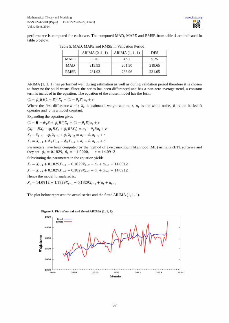
ARIMA (1, 1, 1) has performed well during estimation as well as during validation period therefore it is chosen
to forecast the solid waste. Since the series has been differenced and has a non-zero average trend, a constant
term is included in the equation. The equation of the chosen model has the form:
(1 − 𝜙1𝐵)(1 − 𝐵)𝑑𝑋𝑡 = (1 − 𝜃1𝐵)𝑎𝑡 + 𝑐
Where the first difference d =1; 𝑋𝑡 is estimated weight at time t, 𝑎𝑡 is the white noise, 𝐵 is the backshift
operator and 𝑐 is a model constant.
Expanding the equation gives
(1 − 𝑩 − 𝜙1𝐵 + 𝜙1𝐵2)𝑋𝑡 = (1 − 𝜃1𝐵)𝑎𝑡 + 𝑐
(𝑋𝑡 − 𝑩𝑋𝑡 − 𝜙1𝐵𝑋𝑡 + 𝜙1𝐵2𝑋𝑡) = 𝑎𝑡 − 𝜃1𝐵𝑎𝑡 + 𝑐
𝑋𝑡 − 𝑋𝑡−1 − 𝜙1𝑋𝑡−1 + 𝜙1𝑋𝑡−2 = 𝑎𝑡 − 𝜃1𝑎𝑡−1 + 𝑐
𝑋𝑡 = 𝑋𝑡−1 + 𝜙1𝑋𝑡−1 − 𝜙1𝑋𝑡−2 + 𝑎𝑡 − 𝜃1𝑎𝑡−1 + 𝑐
Parameters have been computed by the method of exact maximum likelihood (ML) using GRETL software and
they are 𝜙1 = 0.1829, 𝜃1 = −1.0000, 𝑐 = 14.0912
Substituting the parameters in the equation yields
𝑋𝑡 = 𝑋𝑡−1 + 0.1829𝑋𝑡−1 − 0.1829𝑋𝑡−2 + 𝑎𝑡 + 𝑎𝑡−1 + 14.0912
𝑋𝑡 = 𝑋𝑡−1 + 0.1829𝑋𝑡−1 − 0.1829𝑋𝑡−2 + 𝑎𝑡 + 𝑎𝑡−1 + 14.0912
Hence the model formulated is:
𝑋𝑡 = 14.0912 + 1.1829𝑋𝑡−1 − 0.1829𝑋𝑡−2 + 𝑎𝑡 + 𝑎𝑡−1
The plot below represent the actual series and the fitted ARIMA (1, 1, 1).
Mathematical Theory and Modeling www.iiste.org
ISSN 2224-5804 (Paper) ISSN 2225-0522 (Online)
Vol.4, No.8, 2014
38
4. Summary and Conclusion
This study analyzed, compared and selected the best time series model for forecasting amount of solid waste
generated in Arusha city among ARIMA and Exponential Smoothing models. The past data used are monthly
amount of solid waste collected by the city authorities from year 2008 to 2013. The data from July 2008 to June
2013 were used to formulate the model and remaining data up to December 2013 were used to validate the
selected potential models. The result indicated that ARIMA (1, 1, 1) outperformed other potential models in
terms of MAPE, MAD and RMSE measures and hence used to forecast the amount of the solid waste generation
for the next years. The forecasted values indicate that by 2018, the monthly generation according to the model
will reach 5100 tons with a 95% confidence interval lying between 4440 – 5750 tons. The model is validated and
is adequate for forecasting solid waste generation and hence results can be used by city authorities to update their
planning of management.
References
Anurag, P. (2008). Forecasting and Model Selection. A paper presented at Reach Symposium, Indian Institute of
Technology, Kanpur, India.
Armstrong, J. S. (2011). Selecting Forecasting Methods. [Online] Available:
http://repository.uppen.edu/marketing_papers/147
Armstrong, J. S. (1985). Long-Range Forecasting, 2nd
Edition. New York: Willey.
Beigl, P. et al. (2003). “Municipal Waste Generation Trends in European Countries and Cities”. Proceedings of
the 9th
International Waste Management and Landfill Symposium. Cagliari, Italy. Oct. 2003. Pg. 6 – 10.
Box, G. E., Jenkins, G. M. and Reinsel, G. C. (2008). Time Series Analysis: Forecasting and Control, Fourth
Edition. Wiley Series in Probability and Statistics, John Wiley & Sons, Inc.
Brockwell, P. J. and Davis, R. A. (2002), Introduction to Time Series and Forecasting, Second Edition, Springer,
New York.
Chung, S. S. (2010). “Projecting Municipal Solid Waste: The Case of Hong Kong SAR”. Resources,
Conservation and Recycling 54.11(2010): Pg. 759-768.
Chatfield, C. (2000). Time – Series Forecasting. Boca Raton, Florida: Chapman and Hall/CRC
Choi, B. (1992). ARMA Model Identification. New York: Springer-Verlag.
Davidson, R. and MacKinnon, G. J. (2004). Econometric Theory and Methods. New York. Oxford University
Press, Inc.
Ebenezer, O., Emmanuel, H., & Ebenezer, B. (2013). Forecasting and Planning for Solid Waste Generation in the
Kumasi Metropolitan Area of Ghana. An ARIMA Time Series Approach. International Journal of Sciences,
Volume 2, Issue April 2013.
Eduardo, O. et al., (2004). A Model for Assessing Waste Generation Factors and Forecasting Waste using
Artificial Neural Networks: A Case Study of Chile. Proceedings of Waste and Recycle2004 Conference.
Freemantle, Australia. Pg. 1-11.
Gardiner, E. S., (1985). Exponential Smoothing: The State of the Art, Journal of forecasting.
Ingrida, R. et al. (2012). “Application and Evaluation of Forecasting Methods for Municipal Solid Waste
Generation in an Eastern European City”. Journal of Waste Management & Research, January 2012, Volume
30, no 1, 89 – 98.
Lyeme H. A., (2011). “Optimization of Municipal Solid Waste Management System: A Case Study of Ilala
Municipality Dar es Salaam”. Masters’ Dissertation. UDSM
Makridakis, S. G. and Wheelwright S. G., (1998). Forecasting: Methods and Applications. 3rd
Edition. John
Wiley & Sons.
Mentzer, J. T and Moon, M. A. (2005). Sales Forecasting Management: A demand Management Approach.
Second Edition. SAGE Publications, Inc.
Mills, T. C., (1990). Time Series Techniques for Economists. London: Cambridge University Press.
Montgomery, D. C., Jennings, C. L. & Kulahci, M. (2008). Introduction to Time Series Analysis and Forecasting.
New Jersey: John Wiley & Sons, Inc.
Montgomery, et al. (1990). Forecasting and Time Series Analysis. New York. McGraw-Hill.
Mathematical Theory and Modeling www.iiste.org
ISSN 2224-5804 (Paper) ISSN 2225-0522 (Online)
Vol.4, No.8, 2014
39
National Bureau of Statistics, (2013). 2012 Population and Housing Census. [Online] Available:
http://www.nbs.go.tz
Narayana, T. (2008). Municipal Solid Waste Management in India: From Waste Disposal to Recovery of
Resources. Waste Management Vol. 29, No.3, pp. 1163 – 1166. [Online] Available:
www.elsevier.com/locate/wasman
Navarro, J et al, (2002). “Time Series Analysis and Forecasting Techniques for Municipal Solid Waste
Management”. Journal of Resource Conservation and Recycling, Volume 35, issue 3 pg. 201-214.
Ni – Bin Chang, (2011). System Analysis for Sustainable Engineering: Theory and Applications. McGraw – Hill
Professional, Access Engineering.
Stevenson, S. (2003). “A Comparison of Forecasting Abilities of ARIMA Models”, Proceeding of Pacific – Rim
Real Estate Society Annual Conference, Brisbane, Australia, January 19-22, 2003.
Simelane, T., & Mohee, R. (2012). Future Directions of Municipality Solid Waste Management in Africa. AISA
POLICY-Brief.
Tsay, R. S. and Tiao, G. C., (1984). “Consistent Estimate of Autoregressive Parameters and Extended Sample
Autocorrelation Function for Stationary and Non-Stationary ARMA Models”. Journal of the American
Statistical Association, Volume 79, pp 84 – 96.
Wei, W. W. S., (1990). Time Series Analysis. Redwood City, CA; Adson Wesley
The IISTE is a pioneer in the Open-Access hosting service and academic event
management. The aim of the firm is Accelerating Global Knowledge Sharing.
More information about the firm can be found on the homepage:
http://www.iiste.org
CALL FOR JOURNAL PAPERS
There are more than 30 peer-reviewed academic journals hosted under the hosting
platform.
Prospective authors of journals can find the submission instruction on the
following page: http://www.iiste.org/journals/ All the journals articles are available
online to the readers all over the world without financial, legal, or technical barriers
other than those inseparable from gaining access to the internet itself. Paper version
of the journals is also available upon request of readers and authors.
MORE RESOURCES
Book publication information: http://www.iiste.org/book/
IISTE Knowledge Sharing Partners
EBSCO, Index Copernicus, Ulrich's Periodicals Directory, JournalTOCS, PKP Open
Archives Harvester, Bielefeld Academic Search Engine, Elektronische
Zeitschriftenbibliothek EZB, Open J-Gate, OCLC WorldCat, Universe Digtial
Library , NewJour, Google Scholar