Embed Size (px)
Citation preview
Time-Series Anomaly Detection Service at MicrosoftHansheng Ren, Bixiong Xu, Yujing Wang, Chao Yi, Congrui Huang, Xiaoyu Kou
∗
Tony Xing, Mao Yang, Jie Tong, Qi Zhang
Microsoft
Beijing, China
{v-hanren,bix,yujwang,t-chyi,conhua,v-xiko,tonyxin,maoyang,jietong,qizhang}@microsoft.com
ABSTRACTLarge companies need to monitor various metrics (for example,
Page Views and Revenue) of their applications and services in real
time. At Microsoft, we develop a time-series anomaly detection ser-
vice which helps customers to monitor the time-series continuously
and alert for potential incidents on time. In this paper, we intro-
duce the pipeline and algorithm of our anomaly detection service,
which is designed to be accurate, efficient and general. The pipeline
consists of three major modules, including data ingestion, exper-
imentation platform and online compute. To tackle the problem
of time-series anomaly detection, we propose a novel algorithm
based on Spectral Residual (SR) and Convolutional Neural Network
(CNN). Our work is the first attempt to borrow the SR model from
visual saliency detection domain to time-series anomaly detection.
Moreover, we innovatively combine SR and CNN together to im-
prove the performance of SRmodel. Our approach achieves superior
experimental results compared with state-of-the-art baselines on
both public datasets and Microsoft production data.
CCS CONCEPTS• Computing methodologies→Machine learning; Unsuper-vised learning; Anomaly detection; • Mathematics of com-puting→ Time series analysis; • Information systems→ Trafficanalysis.
KEYWORDSanomaly detection; time-series; Spectral Residual
ACM Reference Format:Hansheng Ren, Bixiong Xu, Yujing Wang, Chao Yi, Congrui Huang, Xi-
aoyu Kou and Tony Xing, Mao Yang, Jie Tong, Qi Zhang. 2019. Time-
Series Anomaly Detection Service at Microsoft. In The 25th ACM SIGKDDConference on Knowledge Discovery and Data Mining (KDD ’19), August4–8, 2019, Anchorage, AK, USA. ACM, New York, NY, USA, 9 pages. https:
//doi.org/10.1145/3292500.3330680
∗Hansheng Ren is a student in University of Chinese Academy of Sciences; Chao Yi
and Xiaoyu Kou are students in Peking University. The work was done when they
worked as full-time interns at Microsoft.
Permission to make digital or hard copies of all or part of this work for personal or
classroom use is granted without fee provided that copies are not made or distributed
for profit or commercial advantage and that copies bear this notice and the full citation
on the first page. Copyrights for components of this work owned by others than ACM
must be honored. Abstracting with credit is permitted. To copy otherwise, or republish,
to post on servers or to redistribute to lists, requires prior specific permission and/or a
fee. Request permissions from [email protected].
KDD ’19, August 4–8, 2019, Anchorage, AK, USA© 2019 Association for Computing Machinery.
ACM ISBN 978-1-4503-6201-6/19/08. . . $15.00
https://doi.org/10.1145/3292500.3330680
1 INTRODUCTIONAnomaly detection aims to discover unexpected events or rare
items in data. It is popular in many industrial applications and
is an important research area in data mining. Accurate anomaly
detection can trigger prompt troubleshooting, help to avoid loss in
revenue, and maintain the reputation and branding for a company.
For this purpose, large companies have built their own anomaly
detection services to monitor their business, product and service
health [11, 20]. When anomalies are detected, alerts will be sent
to the operators to make timely decisions related to incidents. For
instance, Yahoo releases EGADS [11] to automatically monitor and
raise alerts on millions of time-series of different Yahoo properties
for various use-cases. At Microsoft, we build an anomaly detection
service to monitor millions of metrics coming from Bing, Office
and Azure, which enables engineers move faster in solving live site
issues. In this paper, we focus on the pipeline and algorithm of our
anomaly detection service specialized for time-series data.
There are many challenges in designing an industrial service for
time-series anomaly detection:
Challenge 1: Lack of Labels. To provide anomaly detection
services for a single business scenario, the system must process mil-
lions of time-series simultaneously. There is no easy way for users
to label each time-series manually. Moreover, the data distribution
of time-series is constantly changing, which requires the system
recognizing the anomalies even though similar patterns have not
appeared before. That makes the supervised models insufficient in
the industrial scenario.
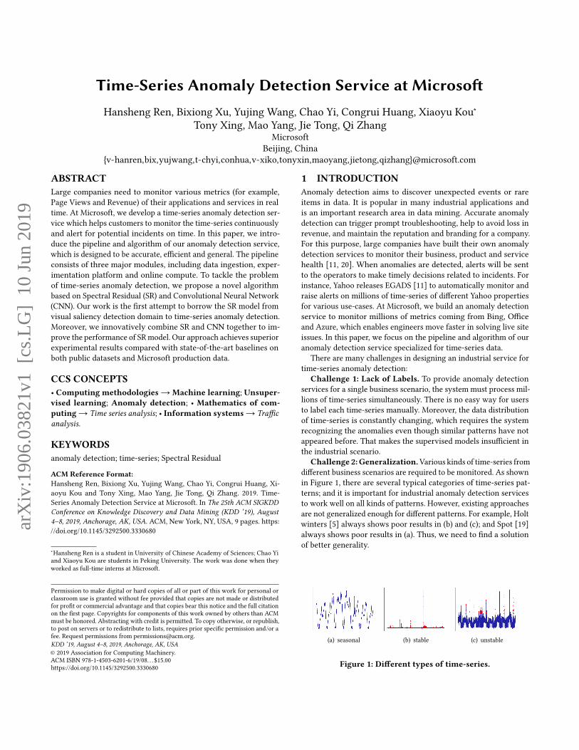
Challenge 2:Generalization.Various kinds of time-series from
different business scenarios are required to be monitored. As shown
in Figure 1, there are several typical categories of time-series pat-
terns; and it is important for industrial anomaly detection services
to work well on all kinds of patterns. However, existing approaches
are not generalized enough for different patterns. For example, Holt
winters [5] always shows poor results in (b) and (c); and Spot [19]
always shows poor results in (a). Thus, we need to find a solution
of better generality.
(a) seasonal (b) stable (c) unstable
Figure 1: Different types of time-series.
arX
iv:1
906.
0382
1v1
[cs
.LG
] 1
0 Ju
n 20
19
Challenge 3: Efficiency. In business applications, a monitor-
ing system must process millions, even billions of time-series in
near real time. Especially for minute-level time-series, the anom-
aly detection procedure needs to be finished within limited time.
Therefore, efficiency is one of the major prerequisites for online
anomaly detection service. Even though the models with large time
complexity are good at accuracy, they are often of little use in an
online scenario.
To tackle the aforementioned problems, our goal is to develop
an anomaly detection approach which is accurate, efficient and
general. Traditional statistical models [5, 14–17, 19, 20, 24] can be
easily adopted online, but their accuracies are not sufficient for
industrial applications. Supervised models [13, 18] are superior in
accuracy, but they are insufficient in our scenario because of lacking
labeled data. There are other unsupervised approaches, for instance,
Luminol [1] and DONUT [23]. However, these methods are either
too time-consuming or parameter-sensitive. Therefore, we aim to
develop a more competitive method in the unsupervised manner
which favors accuracy, efficiency and generality simultaneously.
In this paper, we borrow the Spectral Residual model [10] from
the visual saliency detection domain to our anomaly detection appli-
cation. Spectral Residual (SR) is an efficient unsupervised algorithm,
which demonstrates outstanding performance and robustness in the
visual saliency detection tasks. To the best of our knowledge, our
work is the first attempt to borrow this idea for time-series anomaly
detection. The motivation is that the time-series anomaly detection
task is similar to the problem of visual saliency detection essen-
tially. Saliency is what "stands out" in a photo or scene, enabling
our eye-brain connection to quickly (and essentially unconsciously)
focus on the most important regions. Meanwhile, when anomalies
appear in time-series curves, they are always the most salient part
in vision.
Moreover, we propose a novel approach based on the combina-
tion of SR and CNN. CNN is a state-of-the-art method for supervised
saliency detection when sufficient labeled data is available; while
SR is a state-of-the-art approach in unsupervised setting. Our inno-
vation is to unite these two models by applying CNN on the basis
of SR output directly. As the problem of anomaly discrimination be-
comes much easier upon the output of SR model, we can train CNN
through automatically generated anomalies and achieve significant
performance enhancement over the original SR model. Because the
anomalies used for CNN training is fully synthetic, the SR-CNN ap-
proach remains unsupervised and establishes a new state-of-the-art
performance when no manually labeled data is available.
As shown in the experiments, our proposed algorithm is more
accurate and general than state-of-the-art unsupervised models.
Furthermore, we also apply it as an additional feature in the su-
pervised learning model. The experimental results demonstrate
that the performance can be further improved when labeled data is
available; and the additional features do provide complementary
information to existing anomaly detectors. Up to the date of pa-
per submission, the F1-score of our unsupervised and supervised
approaches are both the best ever achieved on the open datasets.
The contributions of this paper are highlighted as below:
• For the first time in the anomaly detection field, we borrow
the technique of visual saliency detection to detect anomalies
in time-series data. The inspiring results prove the possibil-
ity of using computer vision technologies to solve anomaly
detection problems.
• We combine the SR and CNN model to improve the accuracy
of time-series anomaly detection. The idea is innovative and
the approach outperforms current state-of-the-art methods
by a large margin. Especially, the F1-score is improved by
more than 20% on Microsoft production data.
• From the practical perspective, the proposed solution has
good generality and efficiency. It can be easily integrated
with online monitoring systems to provide quick alerts for
important online metrics. This technique has enabled prod-
uct teams to move faster in detecting issues, save manual
efforts, and accelerate the process of diagnostics.
The rest of this paper is organized as follows. First, in Section 2,
we describe the details of system design, including data ingestion,
experimentation platform and online compute. Then, we share
our experience of real applications in Section 3 and introduce the
methodology in Section 4. Experimental results are analyzed in
Section 5 and related works are presented in Section 6. Finally, we
conclude our work and put forward future work in Section 7.
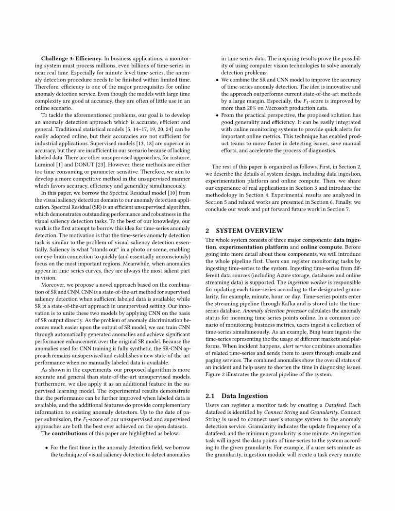
2 SYSTEM OVERVIEWThe whole system consists of three major components: data inges-tion, experimentation platform and online compute. Beforegoing into more detail about these components, we will introduce
the whole pipeline first. Users can register monitoring tasks by
ingesting time-series to the system. Ingesting time-series from dif-
ferent data sources (including Azure storage, databases and online
streaming data) is supported. The ingestion worker is responsiblefor updating each time-series according to the designated granu-
larity, for example, minute, hour, or day. Time-series points enter
the streaming pipeline through Kafka and is stored into the time-
series database. Anomaly detection processor calculates the anomaly
status for incoming time-series points online. In a common sce-
nario of monitoring business metrics, users ingest a collection of
time-series simultaneously. As an example, Bing team ingests the
time-series representing the the usage of different markets and plat-
forms. When incident happens, alert service combines anomalies
of related time-series and sends them to users through emails and
paging services. The combined anomalies show the overall status of
an incident and help users to shorten the time in diagnosing issues.
Figure 2 illustrates the general pipeline of the system.
2.1 Data IngestionUsers can register a monitor task by creating a Datafeed. Eachdatafeed is identified by Connect String and Granularity. ConnectString is used to connect user’s storage system to the anomaly
detection service. Granularity indicates the update frequency of a
datafeed; and the minimum granularity is one minute. An ingestion
task will ingest the data points of time-series to the system accord-
ing to the given granularity. For example, if a user sets minute as
the granularity, ingestion module will create a task every minute
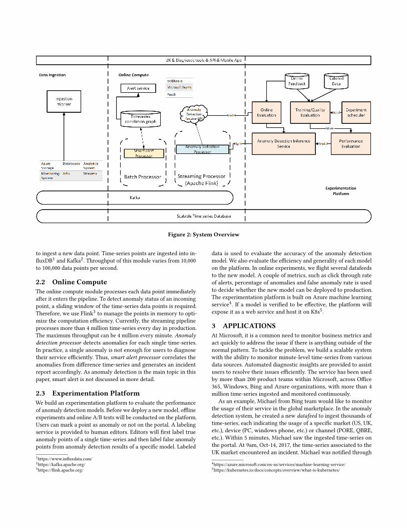
Figure 2: System Overview
to ingest a new data point. Time-series points are ingested into in-
fluxDB1and Kafka
2. Throughput of this module varies from 10,000
to 100,000 data points per second.
2.2 Online ComputeThe online compute module processes each data point immediately
after it enters the pipeline. To detect anomaly status of an incoming
point, a sliding window of the time-series data points is required.
Therefore, we use Flink3to manage the points in memory to opti-
mize the computation efficiency. Currently, the streaming pipeline
processes more than 4 million time-series every day in production.
The maximum throughput can be 4 million every minute. Anomalydetection processor detects anomalies for each single time-series.
In practice, a single anomaly is not enough for users to diagnose
their service efficiently. Thus, smart alert processor correlates theanomalies from difference time-series and generates an incident
report accordingly. As anomaly detection is the main topic in this
paper, smart alert is not discussed in more detail.
2.3 Experimentation PlatformWe build an experimentation platform to evaluate the performance
of anomaly detection models. Before we deploy a newmodel, offline
experiments and online A/B tests will be conducted on the platform.
Users can mark a point as anomaly or not on the portal. A labeling
service is provided to human editors. Editors will first label true
anomaly points of a single time-series and then label false anomaly
points from anomaly detection results of a specific model. Labeled
1https://www.influxdata.com/
2https://kafka.apache.org/
3https://flink.apache.org/
data is used to evaluate the accuracy of the anomaly detection
model. We also evaluate the efficiency and generality of each model
on the platform. In online experiments, we flight several datafeeds
to the new model. A couple of metrics, such as click through rate
of alerts, percentage of anomalies and false anomaly rate is used
to decide whether the new model can be deployed to production.
The experimentation platform is built on Azure machine learning
service4. If a model is verified to be effective, the platform will
expose it as a web service and host it on K8s5.
3 APPLICATIONSAt Microsoft, it is a common need to monitor business metrics and
act quickly to address the issue if there is anything outside of the
normal pattern. To tackle the problem, we build a scalable system
with the ability to monitor minute-level time-series from various
data sources. Automated diagnostic insights are provided to assist
users to resolve their issues efficiently. The service has been used
by more than 200 product teams within Microsoft, across Office
365, Windows, Bing and Azure organizations, with more than 4
million time-series ingested and monitored continuously.
As an example, Michael from Bing team would like to monitor
the usage of their service in the global marketplace. In the anomaly
detection system, he created a new datafeed to ingest thousands of
time-series, each indicating the usage of a specific market (US, UK,
etc.), device (PC, windows phone, etc.) or channel (PORE, QBRE,
etc.). Within 5 minutes, Michael saw the ingested time-series on
the portal. At 9am, Oct-14, 2017, the time-series associated to the
UK market encountered an incident. Michael was notified through
4https://azure.microsoft.com/en-us/services/machine-learning-service/
5https://kubernetes.io/docs/concepts/overview/what-is-kubernetes/
(a) Alert Page (b) Incident Report
Figure 3: An illustration of example application from Microsoft Bing
E-mail alerts (as shown in Figure 3(a)) and started to investigate the
problem. He opened the incident report where the top correlated
time-series with anomalies are selected from a set of time-series
around 9am. As shown in Figure 3(b), usage on PC devices and
PORE channel can be found in the incident report. Michael brought
this insight to the team and finally found that the problem was
caused by a relevance issue which made users do lots of pagination
requests (PORE) to get satisfactory search results.
As another example, the Outlook anti-spam team used to lever-
age a rule-based method to monitor the effectiveness of their spam
detection system. However, this method was not easy to be main-
tained and usually showed bad cases on some Geo-locations. There-
fore, they ingested key metrics to our anomaly detection service
to monitor the effectiveness of their spam detection model across
different Geo-locations. Through our API, they have integrated
anomaly detection ability into the Office DevOps platform. By
using this automatic detection service, they have covered more
Geo-locations and received less false positive cases compared to
the original rule-based solution.
4 METHODOLOGYThe problem of time-series anomaly detection is defined as below.
Problem 1. Given a sequence of real values, i.e., x = x1,x2, ...,xn ,the task of time-series anomaly detection is to produce an outputsequence, y = y1,y2, ...,yn , where yi ∈ {0, 1} denotes whether xi isan anomaly point.
As emphasized in the Introduction, our challenge is to develop
a general and efficient algorithm with no labeled data. Inspired
by the domain of visual computing, we adopt Spectral Residual
(SR) [10], a simple yet powerful approach based on Fast Fourier
Transform (FFT) [21]. The SR approach is unsupervised and has
been proved to be efficient and effective in visual saliency detection
applications. We believe that the visual saliency detection and time-
series anomaly detection tasks are similar essentially, because the
anomaly points are usually salient in the visual perspective.
Furthermore, recent saliency detection research has shown fa-
vor to end-to-end training with Convolutional Neural Networks
(CNNs) when sufficient labeled data is available [25]. Nevertheless,
it is prohibitive for our application as large-scale labeled data is
difficult to be collected online. As a trade-off, we propose a novel
method, SR-CNN, which applies CNN on the output of SR model di-
rectly. CNN is responsible to learn a discriminate rule to replace the
single threshold adopted by the original SR solution. The problem
becomes much easier to learn the CNN model on SR results than
on the original input sequence. Specifically, we can use artificially
generated anomaly labels to train the CNN-based discriminator.
In the following sub-sections, we introduce the details of SR and
SR-CNN methods respectively.
4.1 SR (Spectral Residual)The Spectral Residual (SR) algorithm consists of three major steps:
(1) Fourier Transform to get the log amplitude spectrum; (2) calcu-
lation of spectral residual; and (3) Inverse Fourier Transform that
transforms the sequence back to spatial domain. Mathematically,
given a sequence x, we have
A(f ) = Amplitude(F(x)) (1)
P(f ) = Phrase(F(x)) (2)
L(f ) = loд(A(f )) (3)
AL(f ) = hq (f ) · L(f ) (4)
R(f ) = L(f ) −AL(f ) (5)
S(x) = F−1(exp(R(f ) + iP(f ))) (6)
where F and F−1 denote Fourier Transform and Inverse Fourier
Transform respectively. x is the input sequence with shape n × 1;
A(f ) is the amplitude spectrum of sequence x; P(f ) is the corre-sponding phase spectrum of sequence x; L(f ) is the log represen-tation of A(f ); and AL(f ) is the average spectrum of L(f ) whichcan be approximated by convoluting the input sequence by hq (f ),
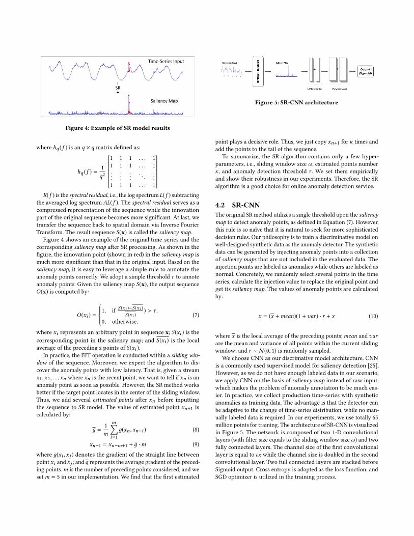
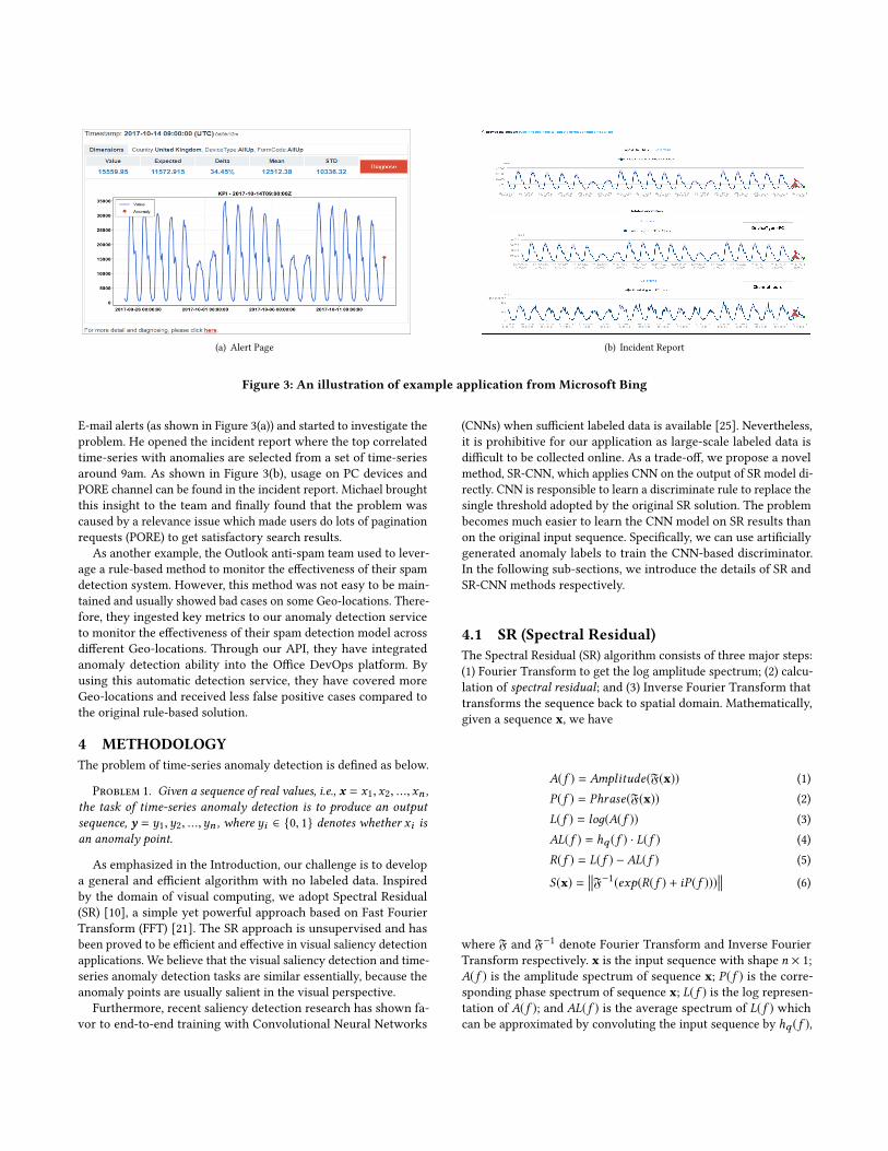
Figure 4: Example of SR model results
where hq (f ) is an q × q matrix defined as:
hq (f ) =1
q2
1 1 1 . . . 1
1 1 1 . . . 1
.......... . .
...
1 1 1 . . . 1
R(f ) is the spectral residual, i.e., the log spectrumL(f ) subtracting
the averaged log spectrum AL(f ). The spectral residual serves as acompressed representation of the sequence while the innovation
part of the original sequence becomes more significant. At last, we
transfer the sequence back to spatial domain via Inverse Fourier
Transform. The result sequence S(x) is called the saliency map.Figure 4 shows an example of the original time-series and the
corresponding saliency map after SR processing. As shown in the
figure, the innovation point (shown in red) in the saliency map is
much more significant than that in the original input. Based on the
saliency map, it is easy to leverage a simple rule to annotate the
anomaly points correctly. We adopt a simple threshold τ to annote
anomaly points. Given the saliency map S(x), the output sequenceO(x) is computed by:
O(xi ) =1, if
S (xi )−S (xi )S (xi )
) > τ ,
0, otherwise,
(7)
where xi represents an arbitrary point in sequence x; S(xi ) is thecorresponding point in the saliency map; and S(xi ) is the local
average of the preceding z points of S(xi ).In practice, the FFT operation is conducted within a sliding win-
dow of the sequence. Moreover, we expect the algorithm to dis-
cover the anomaly points with low latency. That is, given a stream
x1,x2, ...,xn where xn is the recent point, we want to tell if xn is an
anomaly point as soon as possible. However, the SR method works
better if the target point locates in the center of the sliding window.
Thus, we add several estimated points after xn before inputting
the sequence to SR model. The value of estimated point xn+1 is
calculated by:
д =1
m
m∑i=1
д(xn ,xn−i ) (8)
xn+1 = xn−m+1 + д ·m (9)
where д(xi ,x j ) denotes the gradient of the straight line betweenpoint xi and x j ; and д represents the average gradient of the preced-ing points.m is the number of preceding points considered, and we
setm = 5 in our implementation. We find that the first estimated
Figure 5: SR-CNN architecture
point plays a decisive role. Thus, we just copy xn+1 for κ times and
add the points to the tail of the sequence.
To summarize, the SR algorithm contains only a few hyper-
parameters, i.e., sliding window size ω, estimated points number
κ, and anomaly detection threshold τ . We set them empirically
and show their robustness in our experiments. Therefore, the SR
algorithm is a good choice for online anomaly detection service.
4.2 SR-CNNThe original SR method utilizes a single threshold upon the saliencymap to detect anomaly points, as defined in Equation (7). However,
this rule is so naïve that it is natural to seek for more sophisticated
decision rules. Our philosophy is to train a discriminative model on
well-designed synthetic data as the anomaly detector. The synthetic
data can be generated by injecting anomaly points into a collection
of saliency maps that are not included in the evaluated data. The
injection points are labeled as anomalies while others are labeled as
normal. Concretely, we randomly select several points in the time
series, calculate the injection value to replace the original point and
get its saliency map. The values of anomaly points are calculated
by:
x = (x +mean)(1 +var ) · r + x (10)
where x is the local average of the preceding points;mean and varare the mean and variance of all points within the current sliding
window; and r ∼ N(0, 1) is randomly sampled.
We choose CNN as our discrimative model architecture. CNN
is a commonly used supervised model for saliency detection [25].
However, as we do not have enough labeled data in our scenario,
we apply CNN on the basis of saliency map instead of raw input,
which makes the problem of anomaly annotation to be much eas-
ier. In practice, we collect production time-series with synthetic
anomalies as training data. The advantage is that the detector can
be adaptive to the change of time-series distribution, while no man-
ually labeled data is required. In our experiments, we use totally 65
million points for training. The architecture of SR-CNN is visualized
in Figure 5. The network is composed of two 1-D convolutional
layers (with filter size equals to the sliding window size ω) and twofully connected layers. The channel size of the first convolutional
layer is equal to ω; while the channel size is doubled in the second
convolutional layer. Two full connected layers are stacked before
Sigmoid output. Cross entropy is adopted as the loss function; and
SGD optimizer is utilized in the training process.
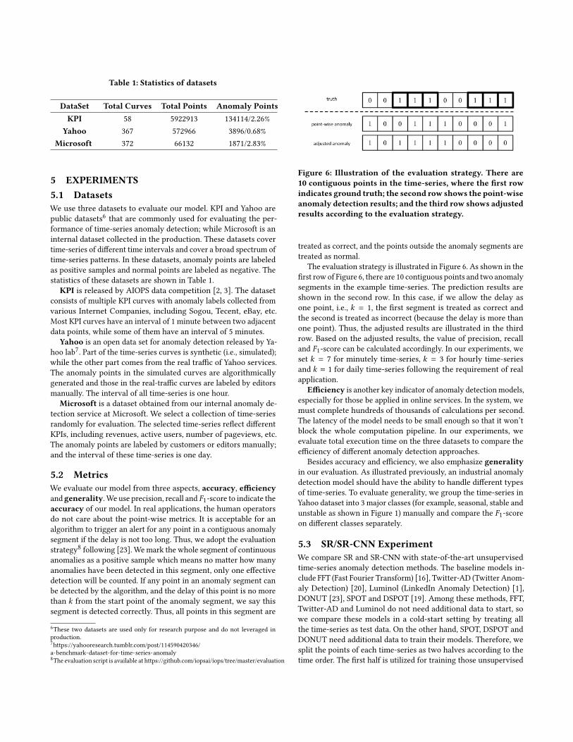
Table 1: Statistics of datasets
DataSet Total Curves Total Points Anomaly PointsKPI 58 5922913 134114/2.26%
Yahoo 367 572966 3896/0.68%
Microsoft 372 66132 1871/2.83%
5 EXPERIMENTS5.1 DatasetsWe use three datasets to evaluate our model. KPI and Yahoo are
public datasets6that are commonly used for evaluating the per-
formance of time-series anomaly detection; while Microsoft is an
internal dataset collected in the production. These datasets cover
time-series of different time intervals and cover a broad spectrum of
time-series patterns. In these datasets, anomaly points are labeled
as positive samples and normal points are labeled as negative. The
statistics of these datasets are shown in Table 1.
KPI is released by AIOPS data competition [2, 3]. The dataset
consists of multiple KPI curves with anomaly labels collected from
various Internet Companies, including Sogou, Tecent, eBay, etc.
Most KPI curves have an interval of 1 minute between two adjacent
data points, while some of them have an interval of 5 minutes.
Yahoo is an open data set for anomaly detection released by Ya-
hoo lab7. Part of the time-series curves is synthetic (i.e., simulated);
while the other part comes from the real traffic of Yahoo services.
The anomaly points in the simulated curves are algorithmically
generated and those in the real-traffic curves are labeled by editors
manually. The interval of all time-series is one hour.
Microsoft is a dataset obtained from our internal anomaly de-
tection service at Microsoft. We select a collection of time-series
randomly for evaluation. The selected time-series reflect different
KPIs, including revenues, active users, number of pageviews, etc.
The anomaly points are labeled by customers or editors manually;
and the interval of these time-series is one day.
5.2 MetricsWe evaluate our model from three aspects, accuracy, efficiencyand generality. We use precision, recall and F1-score to indicate theaccuracy of our model. In real applications, the human operators
do not care about the point-wise metrics. It is acceptable for an
algorithm to trigger an alert for any point in a contiguous anomaly
segment if the delay is not too long. Thus, we adopt the evaluation
strategy8following [23]. Wemark the whole segment of continuous
anomalies as a positive sample which means no matter how many
anomalies have been detected in this segment, only one effective
detection will be counted. If any point in an anomaly segment can
be detected by the algorithm, and the delay of this point is no more
than k from the start point of the anomaly segment, we say this
segment is detected correctly. Thus, all points in this segment are
6These two datasets are used only for research purpose and do not leveraged in
production.
7https://yahooresearch.tumblr.com/post/114590420346/
a-benchmark-dataset-for-time-series-anomaly
8The evaluation script is available at https://github.com/iopsai/iops/tree/master/evaluation
Figure 6: Illustration of the evaluation strategy. There are10 contiguous points in the time-series, where the first rowindicates ground truth; the second row shows the point-wiseanomaly detection results; and the third row shows adjustedresults according to the evaluation strategy.
treated as correct, and the points outside the anomaly segments are
treated as normal.
The evaluation strategy is illustrated in Figure 6. As shown in the
first row of Figure 6, there are 10 contiguous points and two anomaly
segments in the example time-series. The prediction results are
shown in the second row. In this case, if we allow the delay as
one point, i.e., k = 1, the first segment is treated as correct and
the second is treated as incorrect (because the delay is more than
one point). Thus, the adjusted results are illustrated in the third
row. Based on the adjusted results, the value of precision, recall
and F1-score can be calculated accordingly. In our experiments, we
set k = 7 for minutely time-series, k = 3 for hourly time-series
and k = 1 for daily time-series following the requirement of real
application.
Efficiency is another key indicator of anomaly detection models,
especially for those be applied in online services. In the system, we
must complete hundreds of thousands of calculations per second.
The latency of the model needs to be small enough so that it won’t
block the whole computation pipeline. In our experiments, we
evaluate total execution time on the three datasets to compare the
efficiency of different anomaly detection approaches.
Besides accuracy and efficiency, we also emphasize generalityin our evaluation. As illustrated previously, an industrial anomaly
detection model should have the ability to handle different types
of time-series. To evaluate generality, we group the time-series in
Yahoo dataset into 3 major classes (for example, seasonal, stable and
unstable as shown in Figure 1) manually and compare the F1-scoreon different classes separately.
5.3 SR/SR-CNN ExperimentWe compare SR and SR-CNN with state-of-the-art unsupervised
time-series anomaly detection methods. The baseline models in-
clude FFT (Fast Fourier Transform) [16], Twitter-AD (Twitter Anom-
aly Detection) [20], Luminol (LinkedIn Anomaly Detection) [1],
DONUT [23], SPOT and DSPOT [19]. Among these methods, FFT,
Twitter-AD and Luminol do not need additional data to start, so
we compare these models in a cold-start setting by treating all
the time-series as test data. On the other hand, SPOT, DSPOT and
DONUT need additional data to train their models. Therefore, we
split the points of each time-series as two halves according to the
time order. The first half is utilized for training those unsupervised
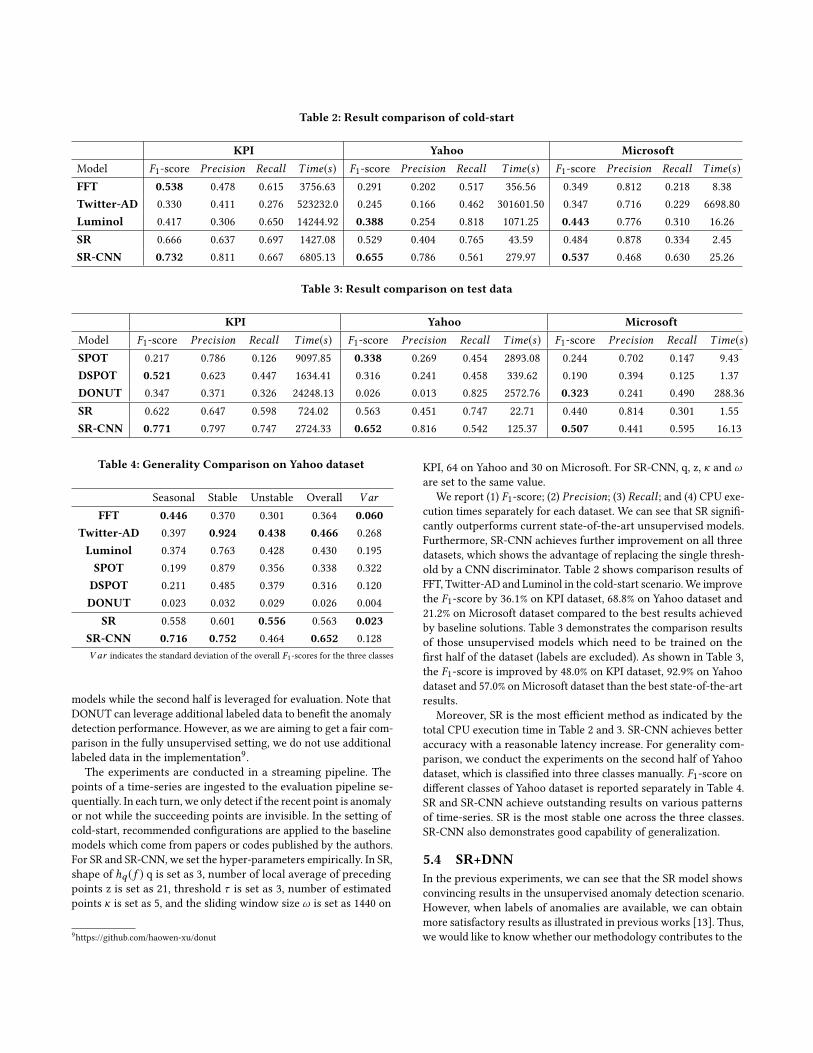
Table 2: Result comparison of cold-start
KPI Yahoo MicrosoftModel F1-score Precision Recall Time(s) F1-score Precision Recall Time(s) F1-score Precision Recall Time(s)FFT 0.538 0.478 0.615 3756.63 0.291 0.202 0.517 356.56 0.349 0.812 0.218 8.38
Twitter-AD 0.330 0.411 0.276 523232.0 0.245 0.166 0.462 301601.50 0.347 0.716 0.229 6698.80
Luminol 0.417 0.306 0.650 14244.92 0.388 0.254 0.818 1071.25 0.443 0.776 0.310 16.26
SR 0.666 0.637 0.697 1427.08 0.529 0.404 0.765 43.59 0.484 0.878 0.334 2.45
SR-CNN 0.732 0.811 0.667 6805.13 0.655 0.786 0.561 279.97 0.537 0.468 0.630 25.26
Table 3: Result comparison on test data
KPI Yahoo MicrosoftModel F1-score Precision Recall Time(s) F1-score Precision Recall Time(s) F1-score Precision Recall Time(s)SPOT 0.217 0.786 0.126 9097.85 0.338 0.269 0.454 2893.08 0.244 0.702 0.147 9.43
DSPOT 0.521 0.623 0.447 1634.41 0.316 0.241 0.458 339.62 0.190 0.394 0.125 1.37
DONUT 0.347 0.371 0.326 24248.13 0.026 0.013 0.825 2572.76 0.323 0.241 0.490 288.36
SR 0.622 0.647 0.598 724.02 0.563 0.451 0.747 22.71 0.440 0.814 0.301 1.55
SR-CNN 0.771 0.797 0.747 2724.33 0.652 0.816 0.542 125.37 0.507 0.441 0.595 16.13
Table 4: Generality Comparison on Yahoo dataset
Seasonal Stable Unstable Overall Var
FFT 0.446 0.370 0.301 0.364 0.060Twitter-AD 0.397 0.924 0.438 0.466 0.268
Luminol 0.374 0.763 0.428 0.430 0.195
SPOT 0.199 0.879 0.356 0.338 0.322
DSPOT 0.211 0.485 0.379 0.316 0.120
DONUT 0.023 0.032 0.029 0.026 0.004
SR 0.558 0.601 0.556 0.563 0.023SR-CNN 0.716 0.752 0.464 0.652 0.128
Var indicates the standard deviation of the overall F1-scores for the three classes
models while the second half is leveraged for evaluation. Note that
DONUT can leverage additional labeled data to benefit the anomaly
detection performance. However, as we are aiming to get a fair com-
parison in the fully unsupervised setting, we do not use additional
labeled data in the implementation9.
The experiments are conducted in a streaming pipeline. The
points of a time-series are ingested to the evaluation pipeline se-
quentially. In each turn, we only detect if the recent point is anomaly
or not while the succeeding points are invisible. In the setting of
cold-start, recommended configurations are applied to the baseline
models which come from papers or codes published by the authors.
For SR and SR-CNN, we set the hyper-parameters empirically. In SR,
shape of hq (f ) q is set as 3, number of local average of preceding
points z is set as 21, threshold τ is set as 3, number of estimated
points κ is set as 5, and the sliding window size ω is set as 1440 on
9https://github.com/haowen-xu/donut
KPI, 64 on Yahoo and 30 on Microsoft. For SR-CNN, q, z, κ and ωare set to the same value.
We report (1) F1-score; (2) Precision; (3) Recall ; and (4) CPU exe-
cution times separately for each dataset. We can see that SR signifi-
cantly outperforms current state-of-the-art unsupervised models.
Furthermore, SR-CNN achieves further improvement on all three
datasets, which shows the advantage of replacing the single thresh-
old by a CNN discriminator. Table 2 shows comparison results of
FFT, Twitter-AD and Luminol in the cold-start scenario.We improve
the F1-score by 36.1% on KPI dataset, 68.8% on Yahoo dataset and
21.2% on Microsoft dataset compared to the best results achieved
by baseline solutions. Table 3 demonstrates the comparison results
of those unsupervised models which need to be trained on the
first half of the dataset (labels are excluded). As shown in Table 3,
the F1-score is improved by 48.0% on KPI dataset, 92.9% on Yahoo
dataset and 57.0% onMicrosoft dataset than the best state-of-the-art
results.
Moreover, SR is the most efficient method as indicated by the
total CPU execution time in Table 2 and 3. SR-CNN achieves better
accuracy with a reasonable latency increase. For generality com-
parison, we conduct the experiments on the second half of Yahoo
dataset, which is classified into three classes manually. F1-score ondifferent classes of Yahoo dataset is reported separately in Table 4.
SR and SR-CNN achieve outstanding results on various patterns
of time-series. SR is the most stable one across the three classes.
SR-CNN also demonstrates good capability of generalization.
5.4 SR+DNNIn the previous experiments, we can see that the SR model shows
convincing results in the unsupervised anomaly detection scenario.
However, when labels of anomalies are available, we can obtain
more satisfactory results as illustrated in previous works [13]. Thus,
we would like to know whether our methodology contributes to the
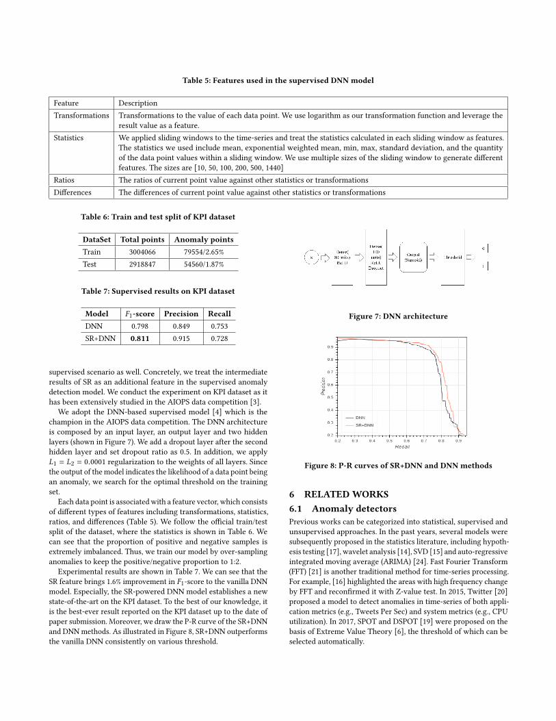
Table 5: Features used in the supervised DNN model
Feature Description
Transformations Transformations to the value of each data point. We use logarithm as our transformation function and leverage the
result value as a feature.
Statistics We applied sliding windows to the time-series and treat the statistics calculated in each sliding window as features.
The statistics we used include mean, exponential weighted mean, min, max, standard deviation, and the quantity
of the data point values within a sliding window. We use multiple sizes of the sliding window to generate different
features. The sizes are [10, 50, 100, 200, 500, 1440]
Ratios The ratios of current point value against other statistics or transformations
Differences The differences of current point value against other statistics or transformations
Table 6: Train and test split of KPI dataset
DataSet Total points Anomaly pointsTrain 3004066 79554/2.65%
Test 2918847 54560/1.87%
Table 7: Supervised results on KPI dataset
Model F1-score Precision RecallDNN 0.798 0.849 0.753
SR+DNN 0.811 0.915 0.728
supervised scenario as well. Concretely, we treat the intermediate
results of SR as an additional feature in the supervised anomaly
detection model. We conduct the experiment on KPI dataset as it
has been extensively studied in the AIOPS data competition [3].
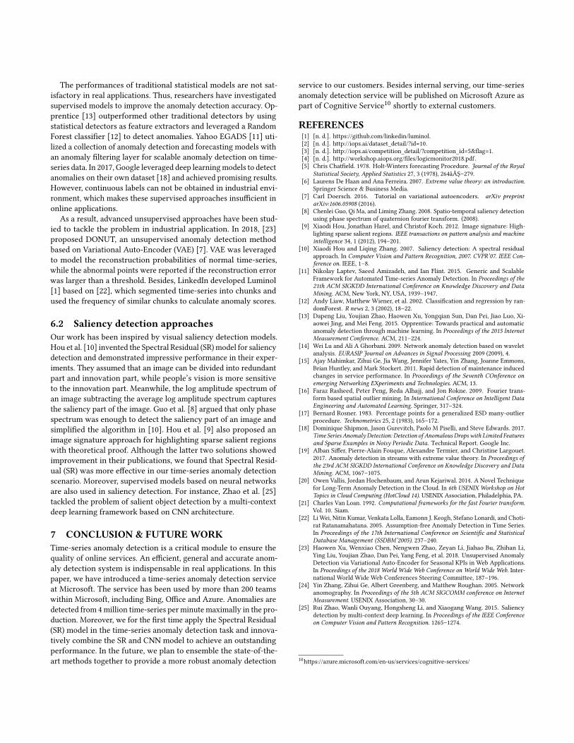
We adopt the DNN-based supervised model [4] which is the
champion in the AIOPS data competition. The DNN architecture
is composed by an input layer, an output layer and two hidden
layers (shown in Figure 7). We add a dropout layer after the second
hidden layer and set dropout ratio as 0.5. In addition, we apply
L1 = L2 = 0.0001 regularization to the weights of all layers. Since
the output of the model indicates the likelihood of a data point being
an anomaly, we search for the optimal threshold on the training
set.
Each data point is associated with a feature vector, which consists
of different types of features including transformations, statistics,
ratios, and differences (Table 5). We follow the official train/test
split of the dataset, where the statistics is shown in Table 6. We
can see that the proportion of positive and negative samples is
extremely imbalanced. Thus, we train our model by over-sampling
anomalies to keep the positive/negative proportion to 1:2.
Experimental results are shown in Table 7. We can see that the
SR feature brings 1.6% improvement in F1-score to the vanilla DNNmodel. Especially, the SR-powered DNN model establishes a new
state-of-the-art on the KPI dataset. To the best of our knowledge, it
is the best-ever result reported on the KPI dataset up to the date of
paper submission. Moreover, we draw the P-R curve of the SR+DNN
and DNNmethods. As illustrated in Figure 8, SR+DNN outperforms
the vanilla DNN consistently on various threshold.
Figure 7: DNN architecture
Figure 8: P-R curves of SR+DNN and DNN methods
6 RELATEDWORKS6.1 Anomaly detectorsPrevious works can be categorized into statistical, supervised and
unsupervised approaches. In the past years, several models were
subsequently proposed in the statistics literature, including hypoth-
esis testing [17], wavelet analysis [14], SVD [15] and auto-regressive
integrated moving average (ARIMA) [24]. Fast Fourier Transform
(FFT) [21] is another traditional method for time-series processing.
For example, [16] highlighted the areas with high frequency change
by FFT and reconfirmed it with Z-value test. In 2015, Twitter [20]
proposed a model to detect anomalies in time-series of both appli-
cation metrics (e.g., Tweets Per Sec) and system metrics (e.g., CPU
utilization). In 2017, SPOT and DSPOT [19] were proposed on the
basis of Extreme Value Theory [6], the threshold of which can be
selected automatically.
The performances of traditional statistical models are not sat-
isfactory in real applications. Thus, researchers have investigated
supervised models to improve the anomaly detection accuracy. Op-
prentice [13] outperformed other traditional detectors by using
statistical detectors as feature extractors and leveraged a Random
Forest classifier [12] to detect anomalies. Yahoo EGADS [11] uti-
lized a collection of anomaly detection and forecasting models with
an anomaly filtering layer for scalable anomaly detection on time-
series data. In 2017, Google leveraged deep learningmodels to detect
anomalies on their own dataset [18] and achieved promising results.
However, continuous labels can not be obtained in industrial envi-
ronment, which makes these supervised approaches insufficient in
online applications.
As a result, advanced unsupervised approaches have been stud-
ied to tackle the problem in industrial application. In 2018, [23]
proposed DONUT, an unsupervised anomaly detection method
based on Variational Auto-Encoder (VAE) [7]. VAE was leveraged
to model the reconstruction probabilities of normal time-series,
while the abnormal points were reported if the reconstruction error
was larger than a threshold. Besides, LinkedIn developed Luminol
[1] based on [22], which segmented time-series into chunks and
used the frequency of similar chunks to calculate anomaly scores.
6.2 Saliency detection approachesOur work has been inspired by visual saliency detection models.
Hou et al. [10] invented the Spectral Residual (SR)model for saliency
detection and demonstrated impressive performance in their exper-
iments. They assumed that an image can be divided into redundant
part and innovation part, while people’s vision is more sensitive
to the innovation part. Meanwhile, the log amplitude spectrum of
an image subtracting the average log amplitude spectrum captures
the saliency part of the image. Guo et al. [8] argued that only phase
spectrum was enough to detect the saliency part of an image and
simplified the algorithm in [10]. Hou et al. [9] also proposed an
image signature approach for highlighting sparse salient regions
with theoretical proof. Although the latter two solutions showed
improvement in their publications, we found that Spectral Resid-
ual (SR) was more effective in our time-series anomaly detection
scenario. Moreover, supervised models based on neural networks
are also used in saliency detection. For instance, Zhao et al. [25]
tackled the problem of salient object detection by a multi-context
deep learning framework based on CNN architecture.
7 CONCLUSION & FUTUREWORKTime-series anomaly detection is a critical module to ensure the
quality of online services. An efficient, general and accurate anom-
aly detection system is indispensable in real applications. In this
paper, we have introduced a time-series anomaly detection service
at Microsoft. The service has been used by more than 200 teams
within Microsoft, including Bing, Office and Azure. Anomalies are
detected from 4million time-series per minute maximally in the pro-
duction. Moreover, we for the first time apply the Spectral Residual
(SR) model in the time-series anomaly detection task and innova-
tively combine the SR and CNN model to achieve an outstanding
performance. In the future, we plan to ensemble the state-of-the-
art methods together to provide a more robust anomaly detection
service to our customers. Besides internal serving, our time-series
anomaly detection service will be published on Microsoft Azure as
part of Cognitive Service10
shortly to external customers.
REFERENCES[1] [n. d.]. https://github.com/linkedin/luminol.
[2] [n. d.]. http://iops.ai/dataset_detail/?id=10.
[3] [n. d.]. http://iops.ai/competition_detail/?competition_id=5&flag=1.
[4] [n. d.]. http://workshop.aiops.org/files/logicmonitor2018.pdf.
[5] Chris Chatfield. 1978. Holt-Winters forecasting Procedure. Journal of the RoyalStatistical Society, Applied Statistics 27, 3 (1978), 264âĂŞ–279.
[6] Laurens De Haan and Ana Ferreira. 2007. Extreme value theory: an introduction.Springer Science & Business Media.
[7] Carl Doersch. 2016. Tutorial on variational autoencoders. arXiv preprintarXiv:1606.05908 (2016).
[8] Chenlei Guo, Qi Ma, and Liming Zhang. 2008. Spatio-temporal saliency detection
using phase spectrum of quaternion fourier transform. (2008).
[9] Xiaodi Hou, Jonathan Harel, and Christof Koch. 2012. Image signature: High-
lighting sparse salient regions. IEEE transactions on pattern analysis and machineintelligence 34, 1 (2012), 194–201.
[10] Xiaodi Hou and Liqing Zhang. 2007. Saliency detection: A spectral residual
approach. In Computer Vision and Pattern Recognition, 2007. CVPR’07. IEEE Con-ference on. IEEE, 1–8.
[11] Nikolay Laptev, Saeed Amizadeh, and Ian Flint. 2015. Generic and Scalable
Framework for Automated Time-series Anomaly Detection. In Proceedings of the21th ACM SIGKDD International Conference on Knowledge Discovery and DataMining. ACM, New York, NY, USA, 1939–1947.
[12] Andy Liaw, Matthew Wiener, et al. 2002. Classification and regression by ran-
domForest. R news 2, 3 (2002), 18–22.[13] Dapeng Liu, Youjian Zhao, Haowen Xu, Yongqian Sun, Dan Pei, Jiao Luo, Xi-
aowei Jing, and Mei Feng. 2015. Opprentice: Towards practical and automatic
anomaly detection through machine learning. In Proceedings of the 2015 InternetMeasurement Conference. ACM, 211–224.
[14] Wei Lu and Ali A Ghorbani. 2009. Network anomaly detection based on wavelet
analysis. EURASIP Journal on Advances in Signal Processing 2009 (2009), 4.
[15] Ajay Mahimkar, Zihui Ge, Jia Wang, Jennifer Yates, Yin Zhang, Joanne Emmons,
Brian Huntley, and Mark Stockert. 2011. Rapid detection of maintenance induced
changes in service performance. In Proceedings of the Seventh COnference onemerging Networking EXperiments and Technologies. ACM, 13.
[16] Faraz Rasheed, Peter Peng, Reda Alhajj, and Jon Rokne. 2009. Fourier trans-
form based spatial outlier mining. In International Conference on Intelligent DataEngineering and Automated Learning. Springer, 317–324.
[17] Bernard Rosner. 1983. Percentage points for a generalized ESD many-outlier
procedure. Technometrics 25, 2 (1983), 165–172.[18] Dominique Shipmon, Jason Gurevitch, Paolo M Piselli, and Steve Edwards. 2017.
Time Series Anomaly Detection: Detection of Anomalous Drops with Limited Featuresand Sparse Examples in Noisy Periodic Data. Technical Report. Google Inc.
[19] Alban Siffer, Pierre-Alain Fouque, Alexandre Termier, and Christine Largouet.
2017. Anomaly detection in streams with extreme value theory. In Proceedings ofthe 23rd ACM SIGKDD International Conference on Knowledge Discovery and DataMining. ACM, 1067–1075.
[20] Owen Vallis, Jordan Hochenbaum, and Arun Kejariwal. 2014. A Novel Technique
for Long-Term Anomaly Detection in the Cloud. In 6th USENIX Workshop on HotTopics in Cloud Computing (HotCloud 14). USENIX Association, Philadelphia, PA.
[21] Charles Van Loan. 1992. Computational frameworks for the fast Fourier transform.
Vol. 10. Siam.
[22] Li Wei, Nitin Kumar, Venkata Lolla, Eamonn J. Keogh, Stefano Lonardi, and Choti-
rat Ratanamahatana. 2005. Assumption-free Anomaly Detection in Time Series.
In Proceedings of the 17th International Conference on Scientific and StatisticalDatabase Management (SSDBM’2005). 237–240.
[23] Haowen Xu, Wenxiao Chen, Nengwen Zhao, Zeyan Li, Jiahao Bu, Zhihan Li,
Ying Liu, Youjian Zhao, Dan Pei, Yang Feng, et al. 2018. Unsupervised Anomaly
Detection via Variational Auto-Encoder for Seasonal KPIs in Web Applications.
In Proceedings of the 2018 World Wide Web Conference on World Wide Web. Inter-national World Wide Web Conferences Steering Committee, 187–196.
[24] Yin Zhang, Zihui Ge, Albert Greenberg, and Matthew Roughan. 2005. Network
anomography. In Proceedings of the 5th ACM SIGCOMM conference on InternetMeasurement. USENIX Association, 30–30.
[25] Rui Zhao, Wanli Ouyang, Hongsheng Li, and Xiaogang Wang. 2015. Saliency
detection by multi-context deep learning. In Proceedings of the IEEE Conferenceon Computer Vision and Pattern Recognition. 1265–1274.
10https://azure.microsoft.com/en-us/services/cognitive-services/


![Comparison of Unsupervised Anomaly Detection Techniques · a RapidMiner [10] Extension Anomaly Detection was developed that contains several unsupervised anomaly detection techniques](https://img.pdfslide.us/doc/110x75/5b014b8c7f8b9a952f8e25e8/comparison-of-unsupervised-anomaly-detection-rapidminer-10-extension-anomaly-detection.jpg)


![Anomaly Detection: Principles, Benchmarking, Explanation ...web.engr.oregonstate.edu/~tgd/...anomaly-detection... · Towards a Theory of Anomaly Detection [Siddiqui, et al.; UAI 2016]](https://img.pdfslide.us/doc/110x75/5fd8992320a65f059c333c6d/anomaly-detection-principles-benchmarking-explanation-webengr-tgdanomaly-detection.jpg)