Time Series Analysis

Dr. Qingling Wu

UCL Geography

Office: G20 Pearson Building

qingling.wu@ucl.ac.uk

Lecture outline

• Introduction to Time Series Analysis

• Decompose signals:

– Loess, STL

• Modeling Time Series

– Autogressive Integrated Moving Average (ARIMA) Model

– Wavelet & Fourier Analysis

– Principle Component Analysis (for 2D)

Reading list

• Textbooks: – Chandler and Scott (2011). Statistical Methods for Trend Detection and

Analysis in the Environmental Sciences, Wiley, 368pp.

– Hamilton (1994). Time Series Analysis, Princeton University Press, 799pp.

– Jolliffe (2005). Principal component analysis. John Wiley & Sons, Ltd. 290pp.

– Wilks (2011). Statistical Methods in the Atmospheric Sciences, 3rd Ed. Chapter 9 (or Chapter 8 in 2nd Ed.)

– Mudelsee (2010). Climate time series analysis: classical statistical and bootstrap methods. Vol. 42. Springer (Very basic, available at here)

• Journal Articles (Time Series in Geographical and Environmental Studies): – Wavelet:

• Grinsted, Aslak, John C. Moore, and Svetlana Jevrejeva (2004). "Application of the cross wavelet transform and wavelet coherence to geophysical time series."Nonlinear processes in geophysics 11.5/6: 561-566.

– PCA/EOF: • Eastman and Filk. (1993) "Long sequence time series evaluation using standardized

principal components." Photogrammetric Engineering and remote sensing 59.6: 991-996. Link

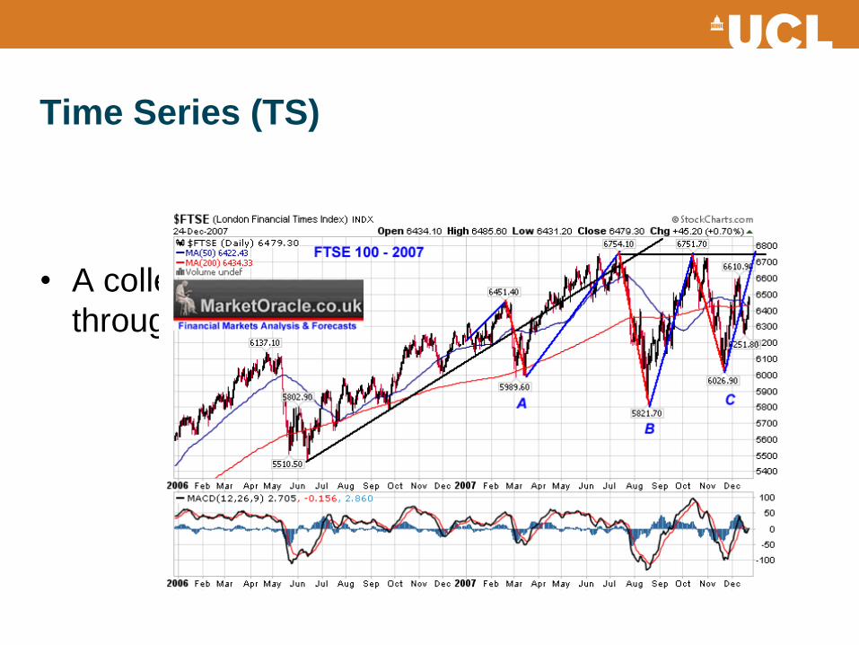
Time Series (TS)

• A collection of observations made sequentially

through time

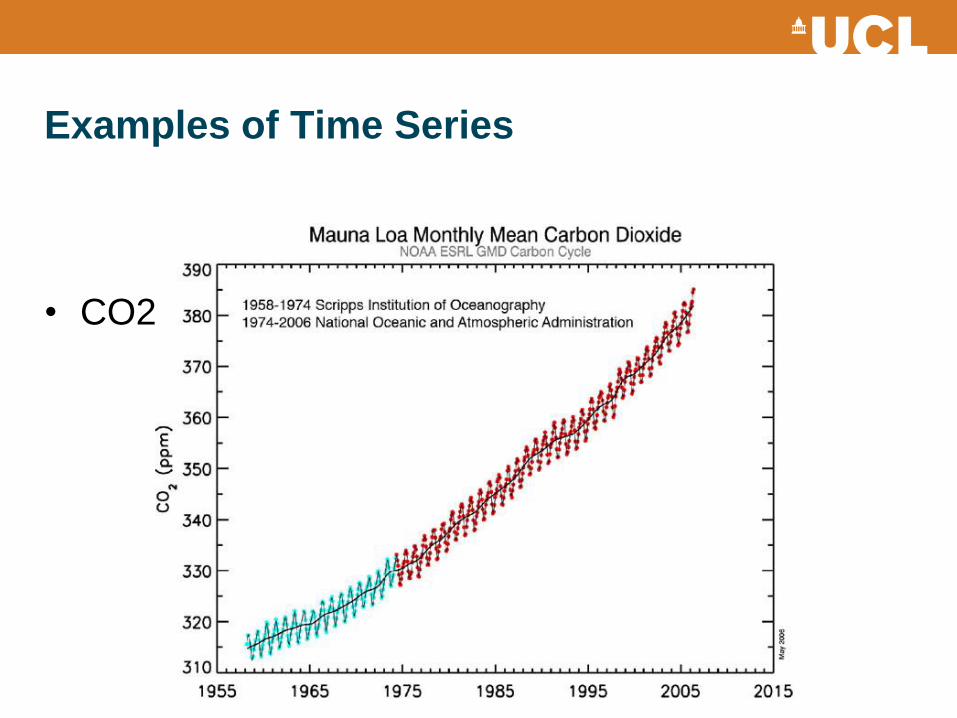
Examples of Time Series

• CO2 emission

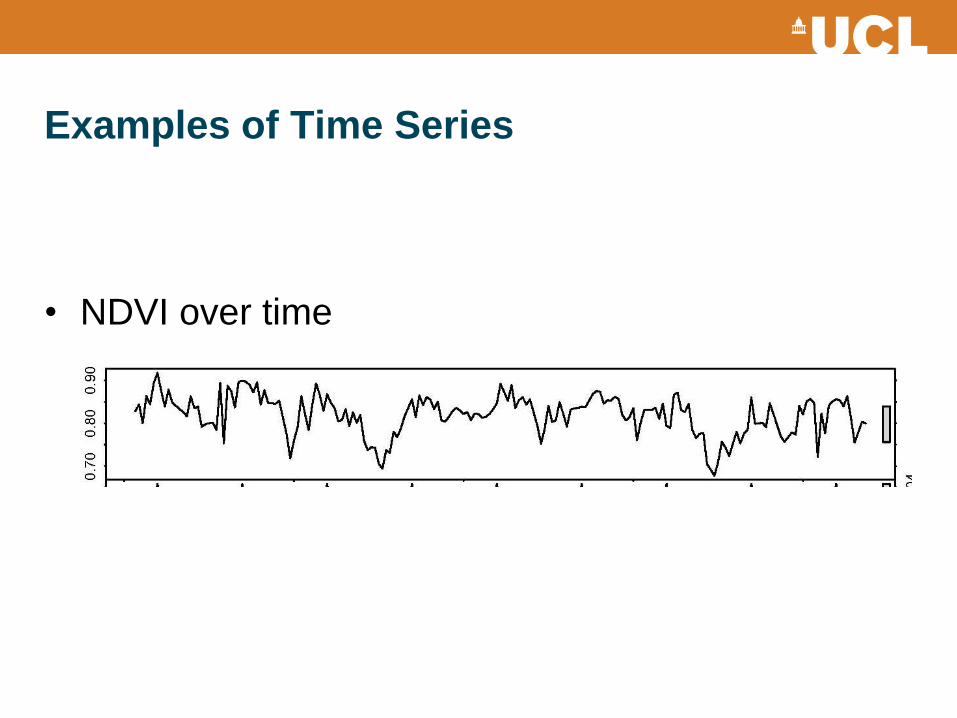
Examples of Time Series

• NDVI over time

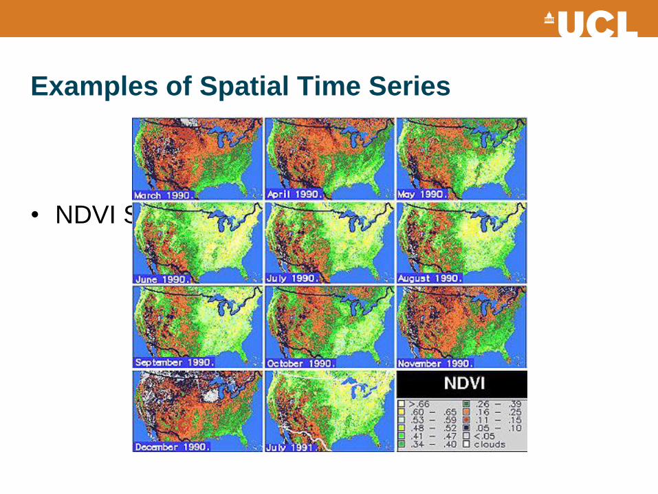
Examples of Spatial Time Series

• NDVI Series over Space and Time

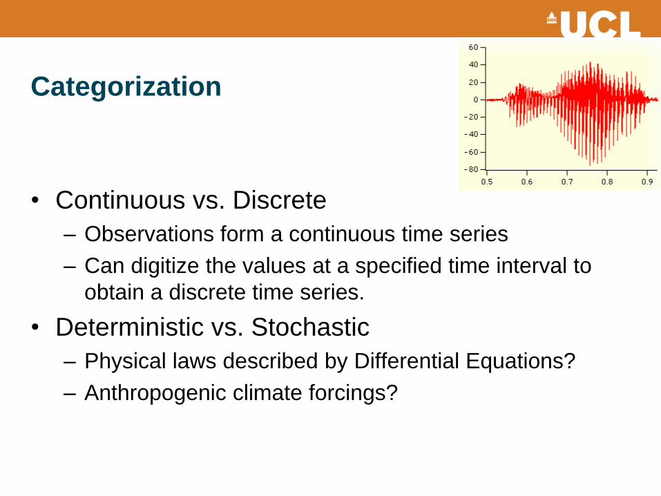
Categorization

• Continuous vs. Discrete

– Observations form a continuous time series

– Can digitize the values at a specified time interval to

obtain a discrete time series.

• Deterministic vs. Stochastic

– Physical laws described by Differential Equations?

– Anthropogenic climate forcings?

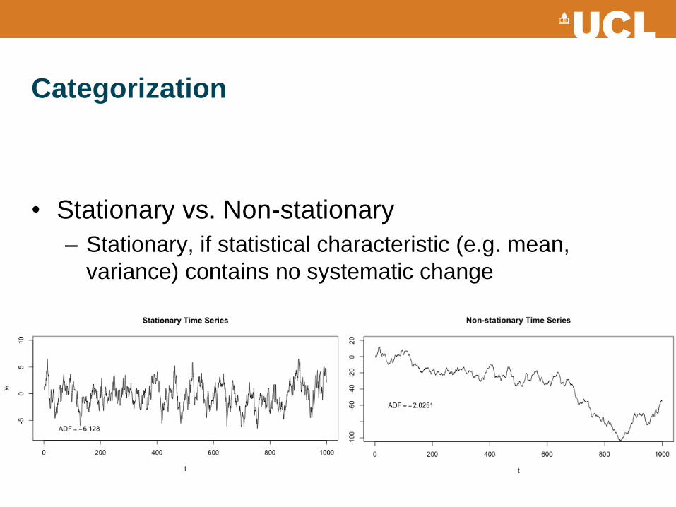
Categorization

• Stationary vs. Non-stationary

– Stationary, if statistical characteristic (e.g. mean,

variance) contains no systematic change

Objectives of Time Series Analysis

• Description – Trend, seasonality/cyclicity, outliers, sudden changes or breaks

• Explanation – Using one TS to explain another

– May help understand the mechanisms

• Prediction – i.e. forecasting

• Control – TS often collected to improve control over a physical process

– Monitoring to alert when conditions exceed an priori determined threshold

Basic Components in a Time Series

• All time-series data have three basic parts:

– A trend component (T)

• Long term change in mean

– A seasonal/cyclic component (S & C)

• Seasonality: i.e. annual variation. Can be deseasonalized

• Cyclicity: variation fixed in period. E.g. diurnal temp. variation

– An irregular component (I)

• Signal after removal of trend and seasonal/cyclic variations

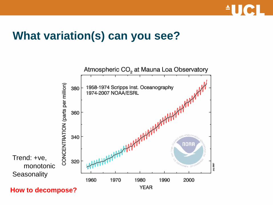
What variation(s) can you see?

How to decompose?

Trend: +ve,

monotonic

Seasonality

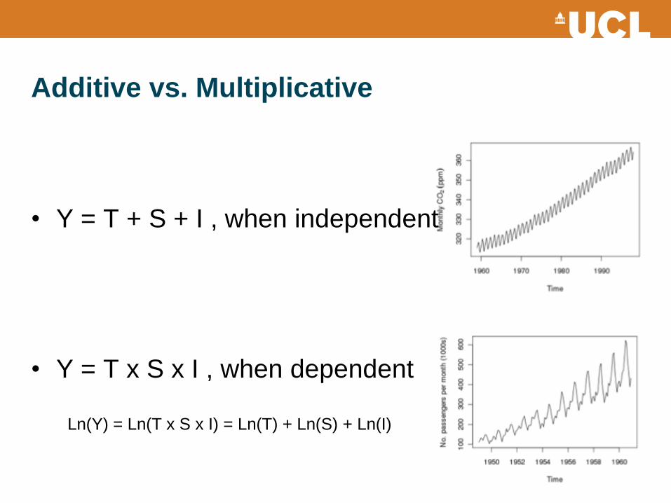
Additive vs. Multiplicative

• Y = T + S + I , when independent

• Y = T x S x I , when dependent

Ln(Y) = Ln(T x S x I) = Ln(T) + Ln(S) + Ln(I)

Smoothing & Fitting

• Smoothing (Convolution)

– Moving Average

– Weighted Moving Average

– Exponential smoothing

• Fitting

– Linear fitting

– Polynomial fitting

– Exponential curve

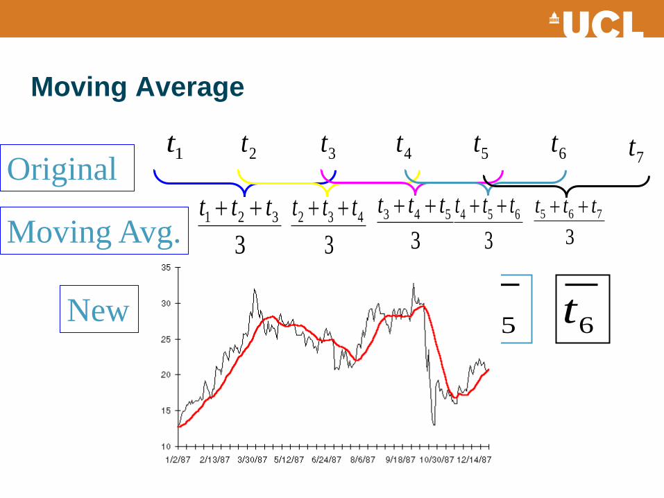
Moving Average

1t 2t 3t 4t 5t 6t 7tOriginal

Moving Avg. 3

321 ttt

3

432 ttt

3

543 ttt

3

654 ttt

3

765 ttt

New 2t 3t 4t 5t 6t

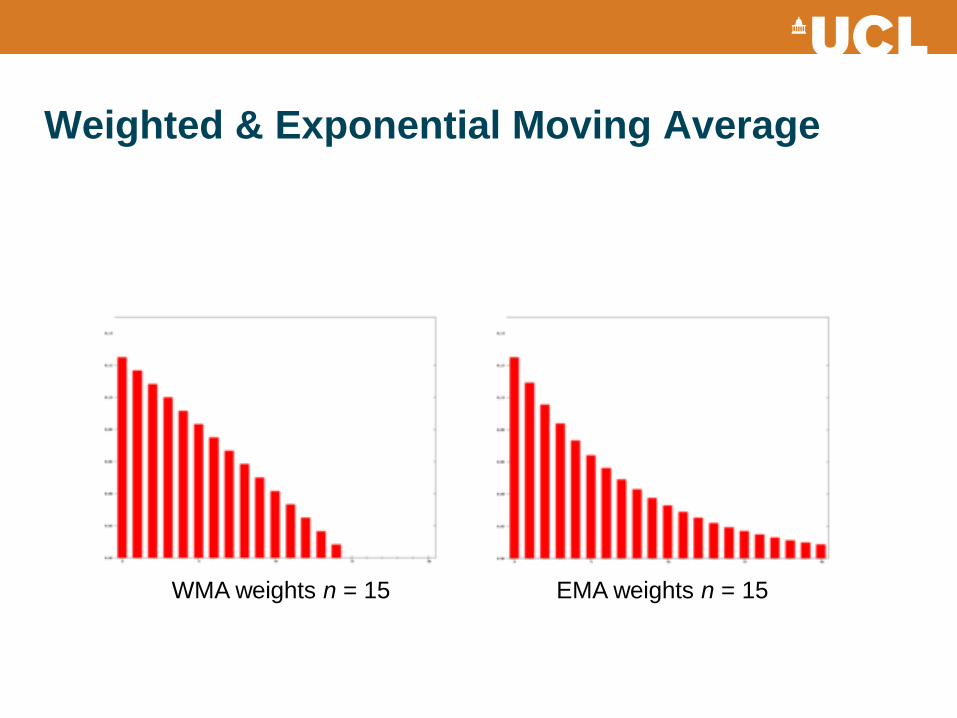
Weighted & Exponential Moving Average

WMA weights n = 15 EMA weights n = 15

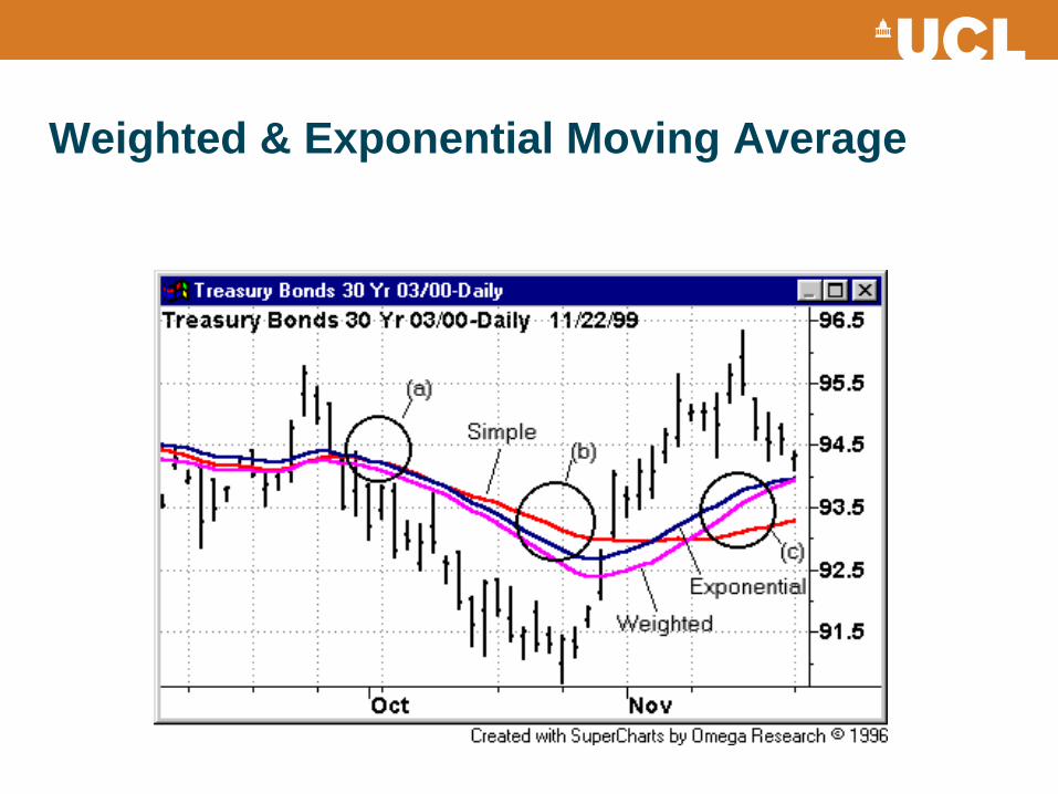
Weighted & Exponential Moving Average

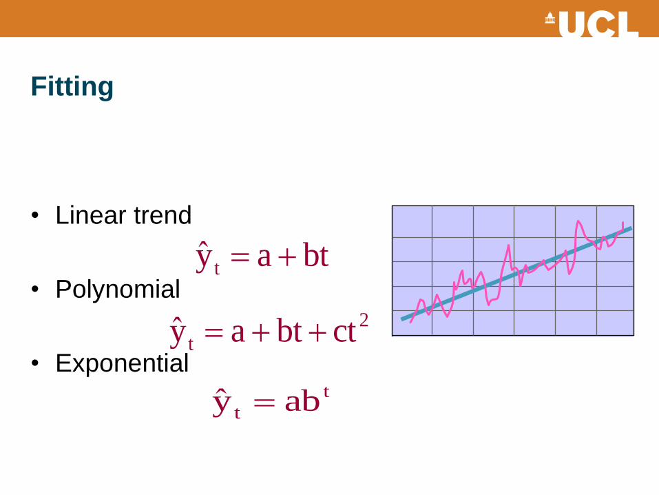
Fitting

• Linear trend

• Polynomial

• Exponential

2

t ctbtay

t

t aby

btay t

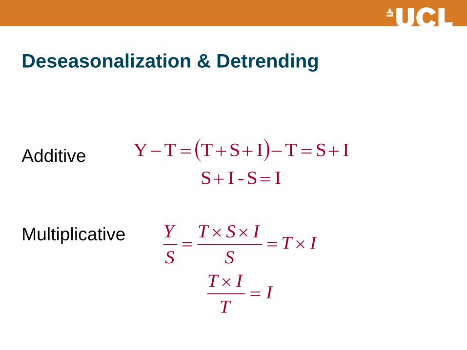
Deseasonalization & Detrending

I S - IS

ISTISTTY

IT

IT

ITS

IST

S

Y

Additive

Multiplicative

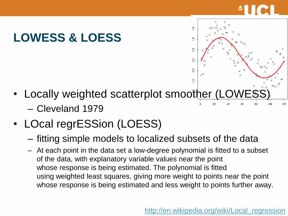
LOWESS & LOESS

• Locally weighted scatterplot smoother (LOWESS)

– Cleveland 1979

• LOcal regrESSion (LOESS)

– fitting simple models to localized subsets of the data – At each point in the data set a low-degree polynomial is fitted to a subset

of the data, with explanatory variable values near the point

whose response is being estimated. The polynomial is fitted

using weighted least squares, giving more weight to points near the point

whose response is being estimated and less weight to points further away.

http://en.wikipedia.org/wiki/Local_regression

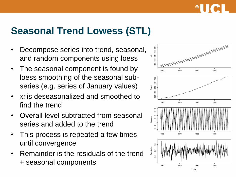
Seasonal Trend Lowess (STL)

• Decompose series into trend, seasonal,

and random components using loess

• The seasonal component is found by

loess smoothing of the seasonal sub-

series (e.g. series of January values)

• xt is deseasonalized and smoothed to

find the trend

• Overall level subtracted from seasonal

series and added to the trend

• This process is repeated a few times

until convergence

• Remainder is the residuals of the trend

+ seasonal components

Autocorrelation

• Autocorrelation

– Correlation between a series and itself (lagged)

– “effective sample size” is reduced in the presence of

+ve autocorrelation

• Autoregression

– whether the next value in the time series can be

predicted as some function of its previous values

Autocorrelation

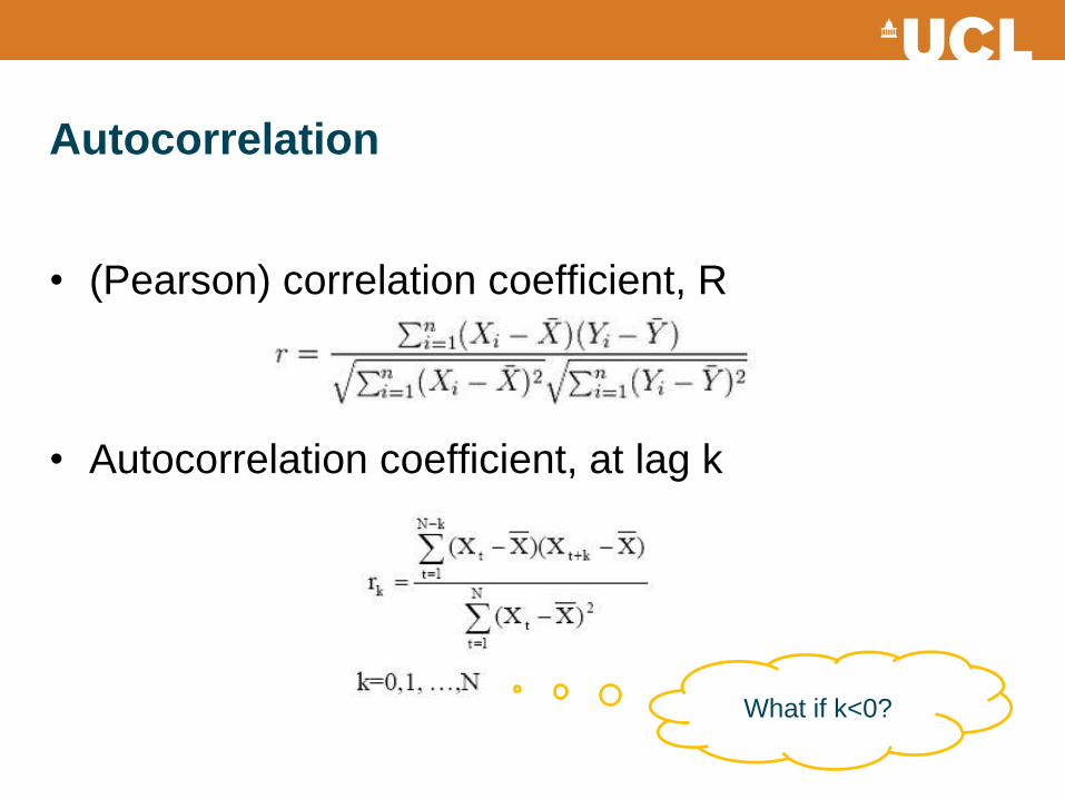
• (Pearson) correlation coefficient, R

• Autocorrelation coefficient, at lag k

What if k<0?

Autocorrelation function (ACF)

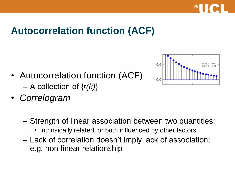
• Autocorrelation function (ACF) – A collection of {r(k)}

• Correlogram

– Strength of linear association between two quantities:

• intrinsically related, or both influenced by other factors

– Lack of correlation doesn’t imply lack of association; e.g. non-linear relationship

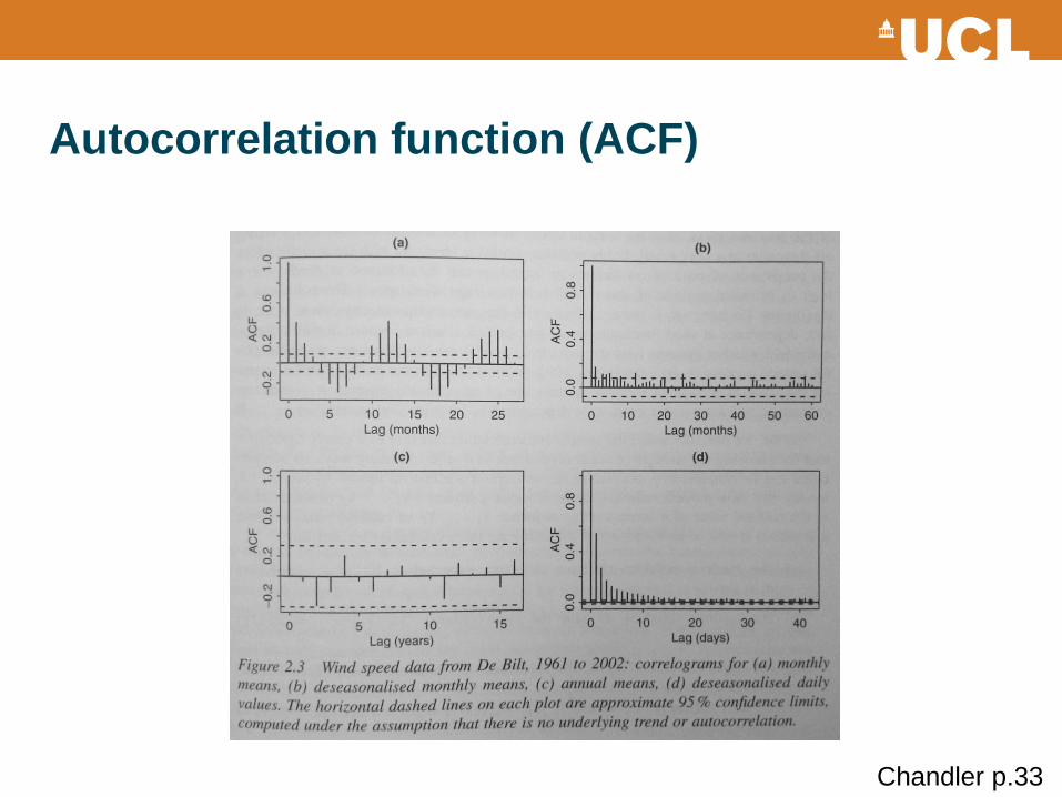
Autocorrelation function (ACF)

Chandler p.33

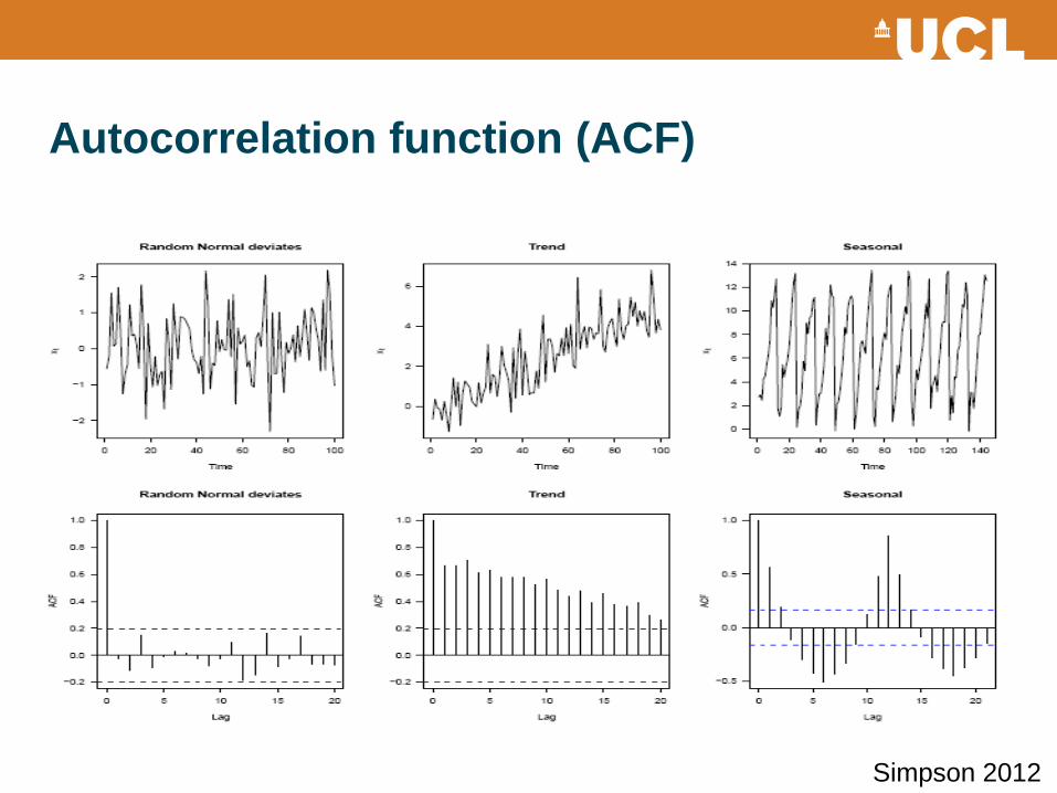
Autocorrelation function (ACF)

Simpson 2012

Partial Autocorrelation function (PACF)

• Wait …

If t0 is correlated with t1, and t1 is correlated with t2,

then to will necessarily be correlated with t2 also…

Partial Autocorrelation function (PACF)

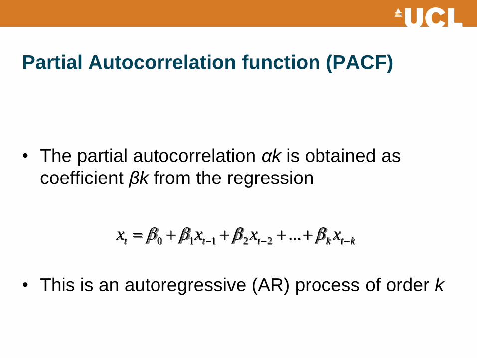
• The partial autocorrelation αk is obtained as

coefficient βk from the regression

• This is an autoregressive (AR) process of order k

ktkttt xxxx ...22110

Partial Autocorrelation function (PACF)

Cross-correlation function (CCF)

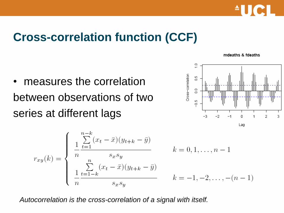
• measures the correlation

between observations of two

series at different lags

Autocorrelation is the cross-correlation of a signal with itself.

Autoregressive (AR) process

• Specifies that the output variable depends linearly

on its own previous values

• AR(p)

– Xt: a function of the past observations plus a purely

random process

– Order p depends on the cutoff on PACF correlogram

– AR(p) process is zero at lag p + 1 and greater

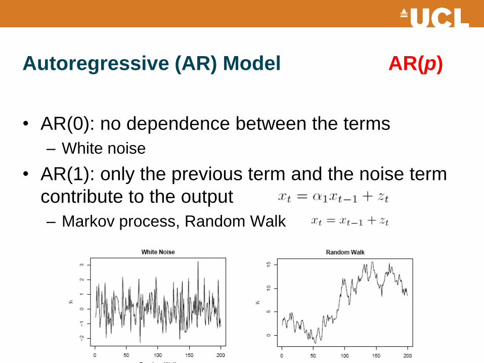
Autoregressive (AR) Model AR(p)

• AR(0): no dependence between the terms

– White noise

• AR(1): only the previous term and the noise term

contribute to the output

– Markov process, Random Walk

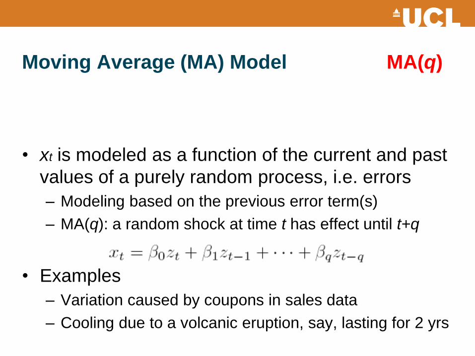
Moving Average (MA) Model MA(q)

• xt is modeled as a function of the current and past

values of a purely random process, i.e. errors

– Modeling based on the previous error term(s)

– MA(q): a random shock at time t has effect until t+q

• Examples

– Variation caused by coupons in sales data

– Cooling due to a volcanic eruption, say, lasting for 2 yrs

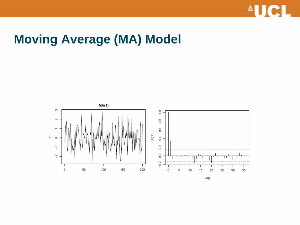
Moving Average (MA) Model

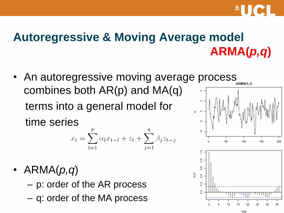
Autoregressive & Moving Average model

ARMA(p,q)

• An autoregressive moving average process

combines both AR(p) and MA(q)

terms into a general model for

time series

• ARMA(p,q)

– p: order of the AR process

– q: order of the MA process

How to choose model orders

• AR and MA signatures: If the PACF displays a

sharp cutoff while the ACF decays more slowly

(i.e., has significant spikes at higher lags), we say

that the stationarized series displays an "AR

signature," meaning that the autocorrelation

pattern can be explained more easily by adding

AR terms than by adding MA terms.

http://people.duke.edu/~rnau/411arim3.htm

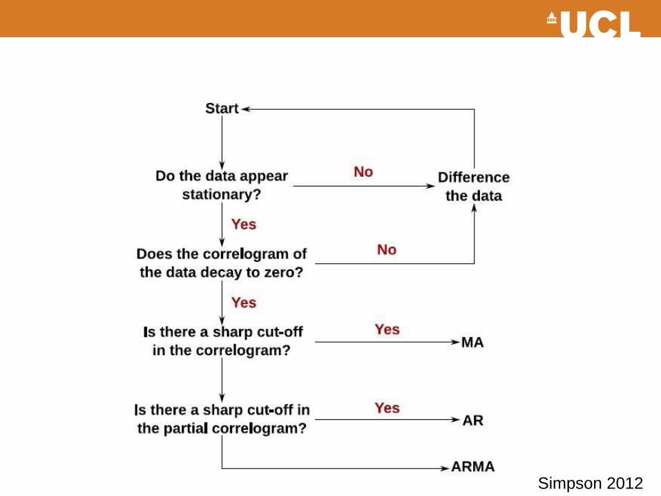
Simpson 2012

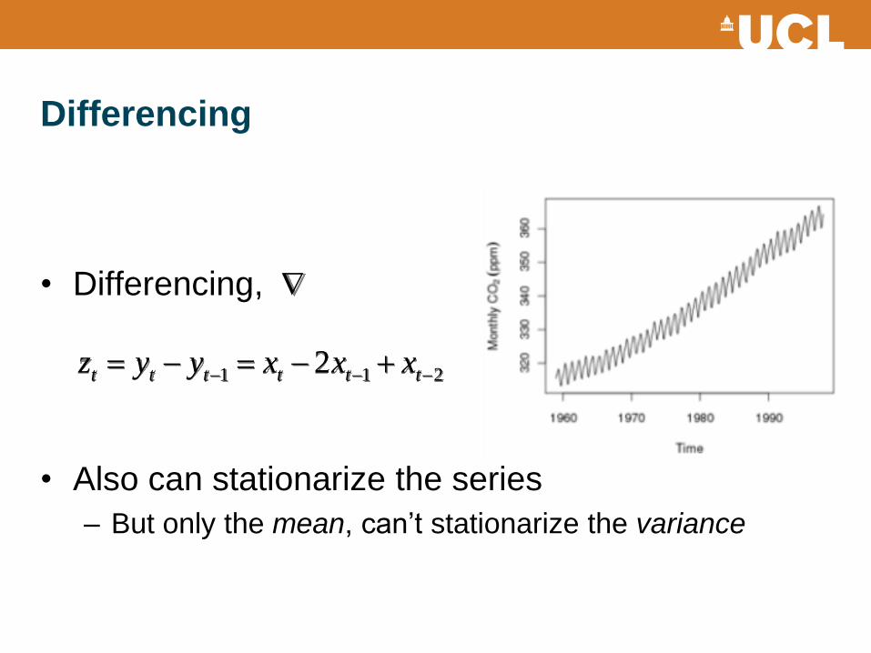
Differencing

• Differencing,

• Also can stationarize the series

– But only the mean, can’t stationarize the variance

211 2 tttttt xxxyyz

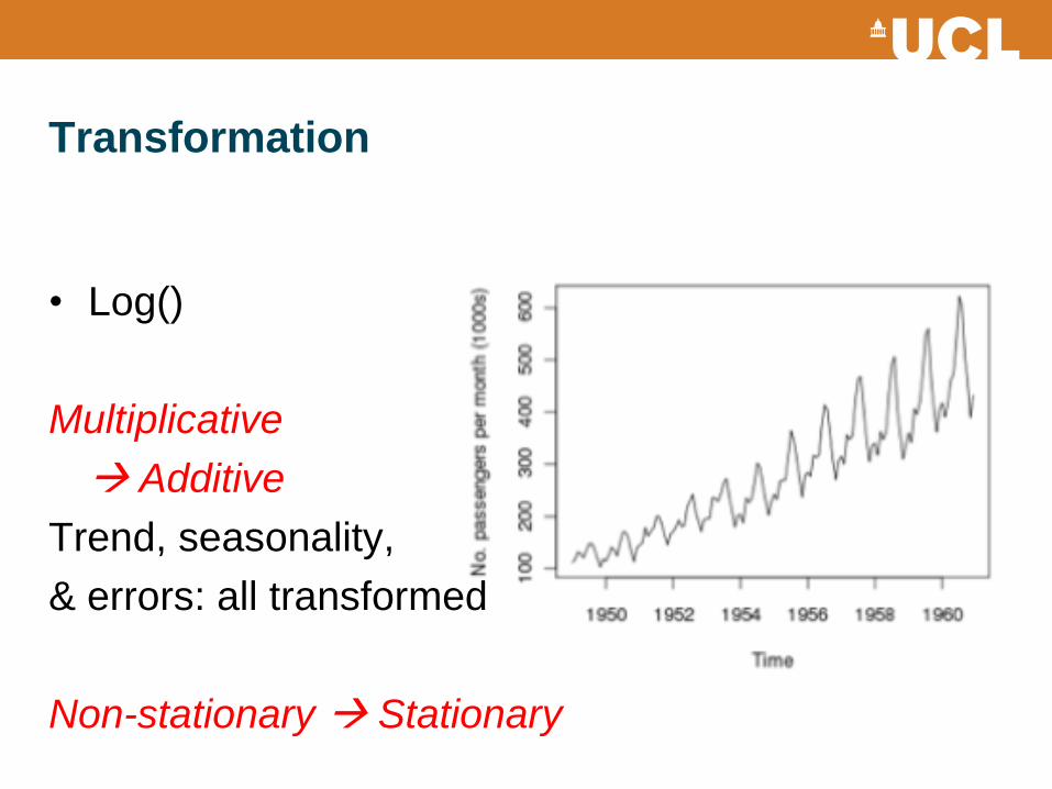
Transformation

• Log()

Multiplicative

Additive

Trend, seasonality,

& errors: all transformed

Non-stationary Stationary

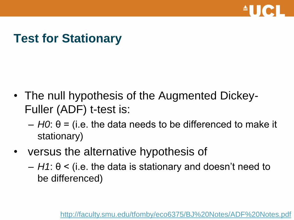
Test for Stationary

• The null hypothesis of the Augmented Dickey-

Fuller (ADF) t-test is:

– H0: θ = (i.e. the data needs to be differenced to make it

stationary)

• versus the alternative hypothesis of

– H1: θ < (i.e. the data is stationary and doesn’t need to

be differenced)

http://faculty.smu.edu/tfomby/eco6375/BJ%20Notes/ADF%20Notes.pdf

ARIMA Model

Thompson UCL

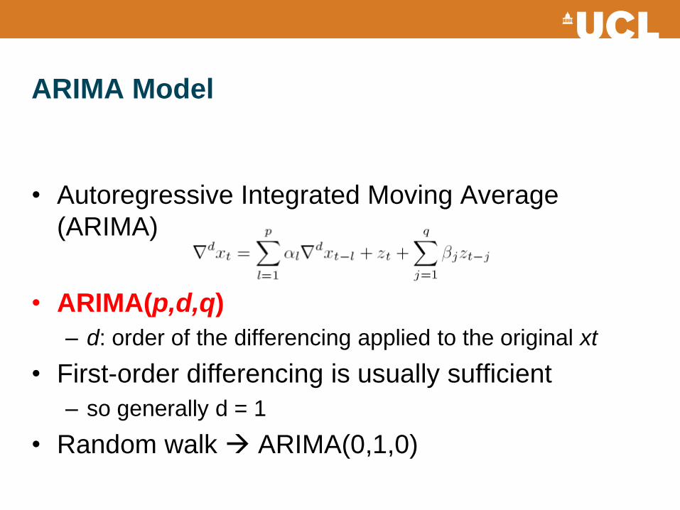
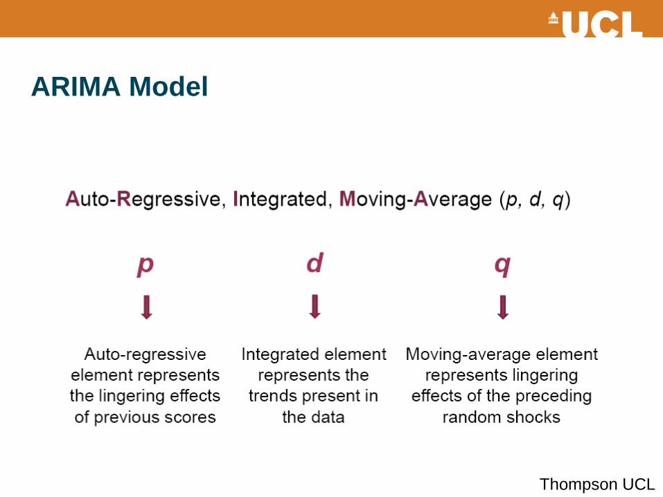
ARIMA Model

• Autoregressive Integrated Moving Average

(ARIMA)

• ARIMA(p,d,q)

– d: order of the differencing applied to the original xt

• First-order differencing is usually sufficient

– so generally d = 1

• Random walk ARIMA(0,1,0)

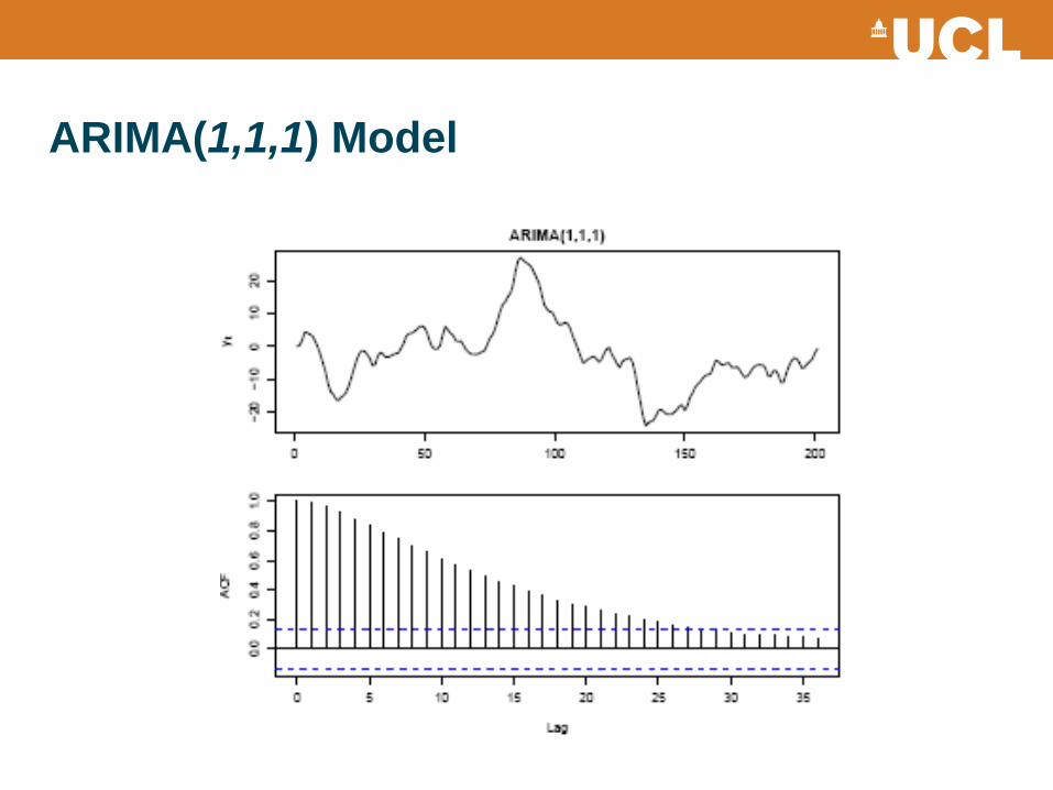
ARIMA(1,1,1) Model

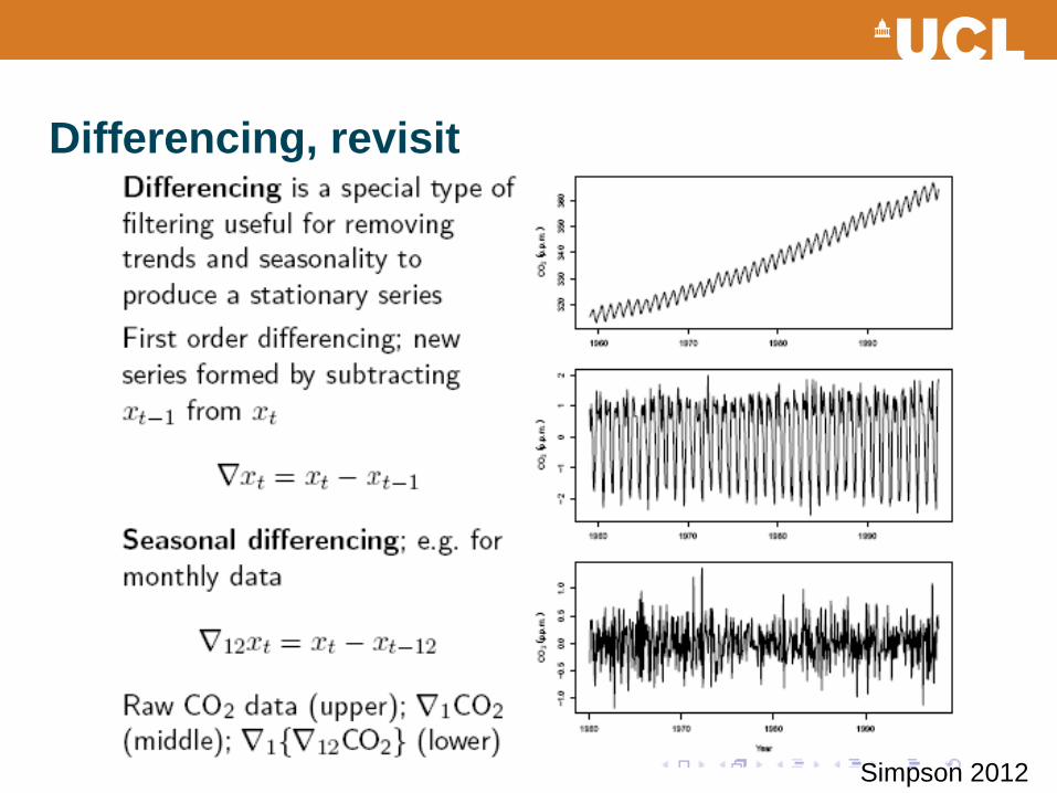
Differencing, revisit

Simpson 2012

Identifying d in ARIMA(p,d,q)

• Once you are happy that the mean and variance

are as constant as possible you can assign d a

value

– If d = 0 the data are stationary and there is no trend;

– If d = 1 the data need to be differenced once so the

linear trend is removed;

– If d = 2 the data need to be difference twice so that the

linear and quadratic trends are removed.

Thompson UCL

Identifying p and q in ARIMA(p,d,q)

• Correlogram

• ACF & PACF Revisit

– ACF: correlation coefficients for consecutive lags

– PACF: partials out the immediate autocorrelations and

estimates the autocorrelation at a specific lag (e.g. 2

lags)

Thomson UCL

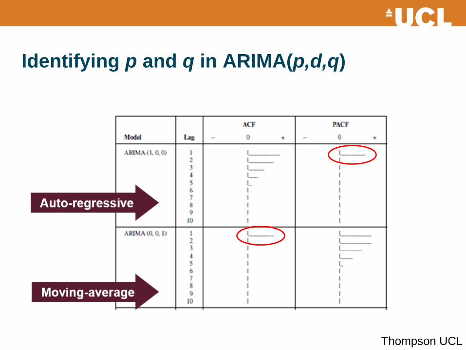
Identifying p and q in ARIMA(p,d,q)

Thompson UCL

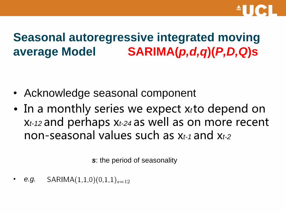
Seasonal autoregressive integrated moving

average Model SARIMA(p,d,q)(P,D,Q)s

• Acknowledge seasonal component

• In a monthly series we expect xt to depend on xt-12 and perhaps xt-24 as well as on more recent non-seasonal values such as xt-1 and xt-2

• e.g.

s: the period of seasonality

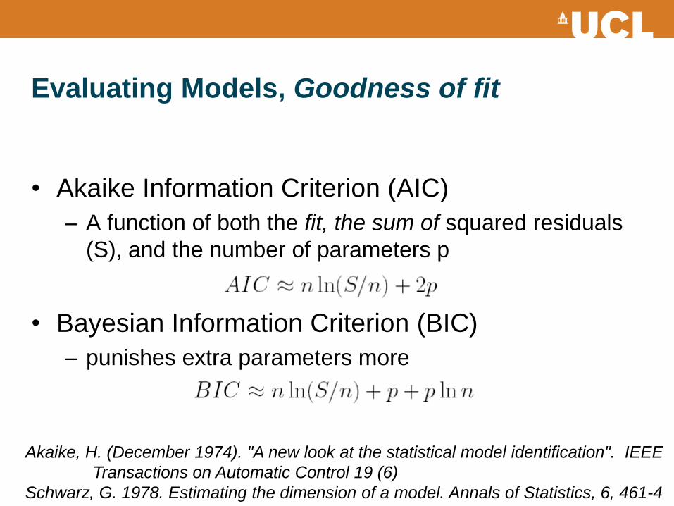
Evaluating Models, Goodness of fit

• Akaike Information Criterion (AIC)

– A function of both the fit, the sum of squared residuals

(S), and the number of parameters p

• Bayesian Information Criterion (BIC)

– punishes extra parameters more

Akaike, H. (December 1974). "A new look at the statistical model identification". IEEE

Transactions on Automatic Control 19 (6)

Schwarz, G. 1978. Estimating the dimension of a model. Annals of Statistics, 6, 461-4

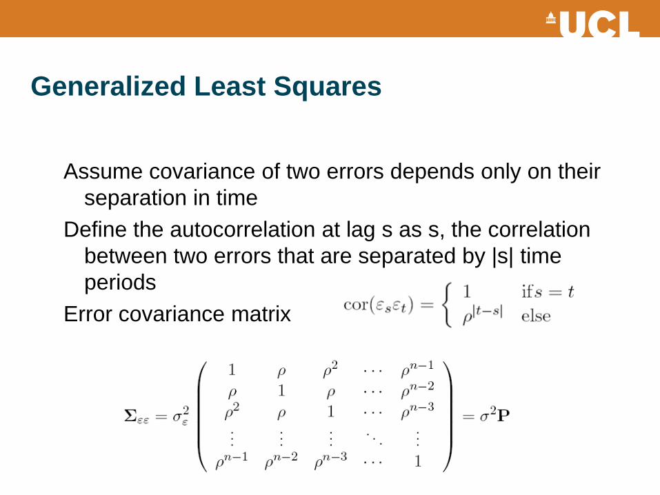
Generalized Least Squares

Assume covariance of two errors depends only on their

separation in time

Define the autocorrelation at lag s as s, the correlation

between two errors that are separated by |s| time

periods

Error covariance matrix

Spectral Analysis

• Period: a repeating pattern in a series

• Sine wave: the fundamental periodic signal

• Joseph Fourier (1768-1830)

– Good approximations to most periodic signals can be

achieved using sums of sine (and cos) waves

• Spectral analysis

– based on sine waves and a decomposition of variation

in series into waves of various frequencies

Fourier Transformation

• Time domain to frequency domain

• Sine wave that makes m cycles in series length is

the mth harmonic

• Amplitude of mth harmonic is

– In general, instead of via a regression, the calculations

above are usually performed with the fast fourier

transform (FFT) algorithm

• Fourier line spectrum: plot of as spikes agst m

22

mmm baA

mA

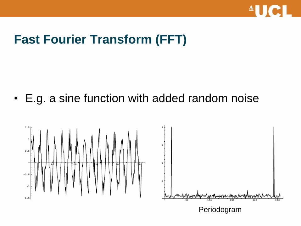
Fast Fourier Transform (FFT)

• E.g. a sine function with added random noise

Periodogram

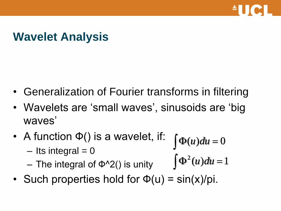
Wavelet Analysis

• Generalization of Fourier transforms in filtering

• Wavelets are ‘small waves’, sinusoids are ‘big

waves’

• A function Ф() is a wavelet, if:

– Its integral = 0

– The integral of Ф^2() is unity

• Such properties hold for Ф(u) = sin(x)/pi.

1)(2 duu

0)( duu

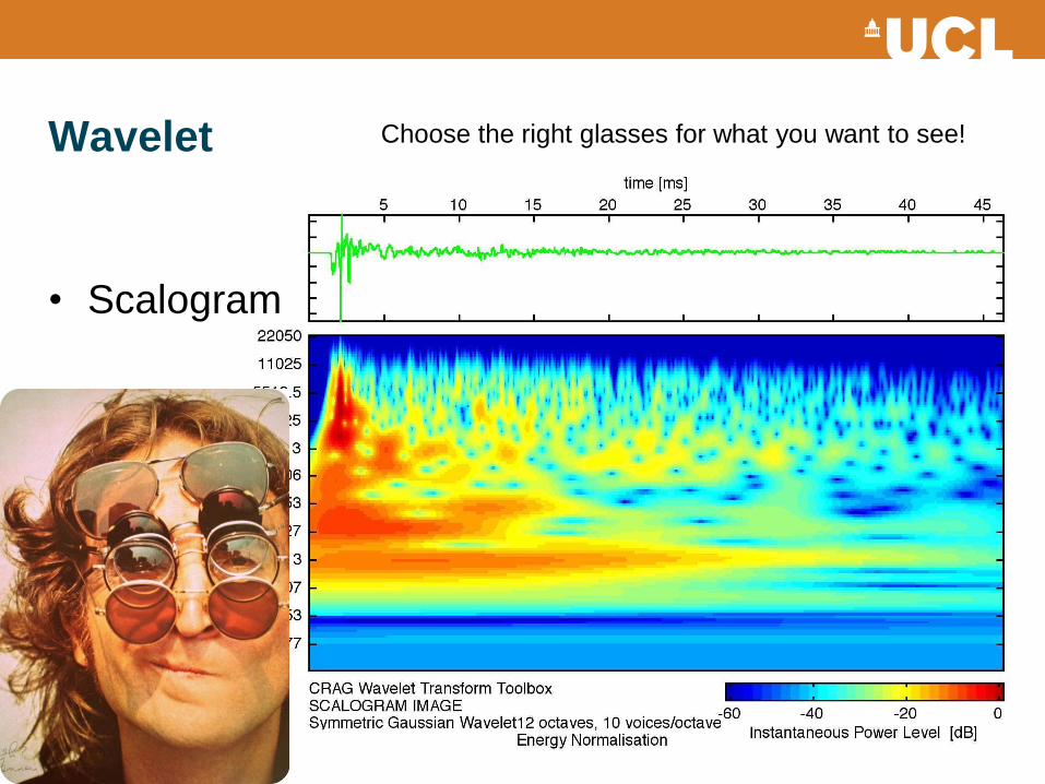
Wavelet

• Scalogram

Choose the right glasses for what you want to see!

Time Series in Remote Sensing

• 1D 2D

• Spatial && Temporal feature extraction

• PCA/EOF

– Principle Component Analysis (Empirical Orthogonal

Function)

Practical

• https://github.com/qwu-hab/geogg121