Embed Size (px)
Citation preview

Time Series AnalysisLecture Notes for 475.726
Ross Ihaka
Statistics DepartmentUniversity of Auckland
April 14, 2005

ii
Contents
1 Introduction 11.1 Time Series . . . . . . . . . . . . . . . . . . . . . . . . . . . . . . 11.2 Stationarity and Non-Stationarity . . . . . . . . . . . . . . . . . 11.3 Some Examples . . . . . . . . . . . . . . . . . . . . . . . . . . . . 2
1.3.1 Annual Auckland Rainfall . . . . . . . . . . . . . . . . . . 21.3.2 Nile River Flow . . . . . . . . . . . . . . . . . . . . . . . . 21.3.3 Yield on British Government Securities . . . . . . . . . . 21.3.4 Ground Displacement in an Earthquake . . . . . . . . . . 31.3.5 United States Housing Starts . . . . . . . . . . . . . . . . 31.3.6 Iowa City Bus Ridership . . . . . . . . . . . . . . . . . . . 3
2 Vector Space Theory 72.1 Vectors In Two Dimensions . . . . . . . . . . . . . . . . . . . . . 7
2.1.1 Scalar Multiplication and Addition . . . . . . . . . . . . . 72.1.2 Norms and Inner Products . . . . . . . . . . . . . . . . . 8
2.2 General Vector Spaces . . . . . . . . . . . . . . . . . . . . . . . . 92.2.1 Vector Spaces and Inner Products . . . . . . . . . . . . . 92.2.2 Some Examples . . . . . . . . . . . . . . . . . . . . . . . . 11
2.3 Hilbert Spaces . . . . . . . . . . . . . . . . . . . . . . . . . . . . 122.3.1 Subspaces . . . . . . . . . . . . . . . . . . . . . . . . . . . 132.3.2 Projections . . . . . . . . . . . . . . . . . . . . . . . . . . 13
2.4 Hilbert Spaces and Prediction . . . . . . . . . . . . . . . . . . . . 142.4.1 Linear Prediction . . . . . . . . . . . . . . . . . . . . . . . 142.4.2 General Prediction . . . . . . . . . . . . . . . . . . . . . . 15
3 Time Series Theory 173.1 Time Series . . . . . . . . . . . . . . . . . . . . . . . . . . . . . . 173.2 Hilbert Spaces and Stationary Time Series . . . . . . . . . . . . . 183.3 The Lag and Differencing Operators . . . . . . . . . . . . . . . . 193.4 Linear Processes . . . . . . . . . . . . . . . . . . . . . . . . . . . 203.5 Autoregressive Series . . . . . . . . . . . . . . . . . . . . . . . . . 21
3.5.1 The AR(1) Series . . . . . . . . . . . . . . . . . . . . . . . 213.5.2 The AR(2) Series . . . . . . . . . . . . . . . . . . . . . . . 233.5.3 Computations . . . . . . . . . . . . . . . . . . . . . . . . . 26
3.6 Moving Average Series . . . . . . . . . . . . . . . . . . . . . . . . 293.6.1 The MA(1) Series . . . . . . . . . . . . . . . . . . . . . . 293.6.2 Invertibility . . . . . . . . . . . . . . . . . . . . . . . . . . 293.6.3 Computation . . . . . . . . . . . . . . . . . . . . . . . . . 30
iii

iv Contents
3.7 Autoregressive Moving Average Series . . . . . . . . . . . . . . . 303.7.1 The ARMA(1,1) Series . . . . . . . . . . . . . . . . . . . 313.7.2 The ARMA(p,q) Model . . . . . . . . . . . . . . . . . . . 323.7.3 Computation . . . . . . . . . . . . . . . . . . . . . . . . . 323.7.4 Common Factors . . . . . . . . . . . . . . . . . . . . . . . 34
3.8 The Partial Autocorrelation Function . . . . . . . . . . . . . . . 343.8.1 Computing the PACF . . . . . . . . . . . . . . . . . . . . 363.8.2 Computation . . . . . . . . . . . . . . . . . . . . . . . . . 37
4 Identifying Time Series Models 394.1 ACF Estimation . . . . . . . . . . . . . . . . . . . . . . . . . . . 394.2 PACF Estimation . . . . . . . . . . . . . . . . . . . . . . . . . . . 424.3 System Identification . . . . . . . . . . . . . . . . . . . . . . . . . 434.4 Model Generalisation . . . . . . . . . . . . . . . . . . . . . . . . . 45
4.4.1 Non-Zero Means . . . . . . . . . . . . . . . . . . . . . . . 454.4.2 Deterministic Trends . . . . . . . . . . . . . . . . . . . . . 474.4.3 Models With Non-stationary AR Components . . . . . . . 474.4.4 The Effect of Differencing . . . . . . . . . . . . . . . . . . 48
4.5 ARIMA Models . . . . . . . . . . . . . . . . . . . . . . . . . . . . 49
5 Fitting and Forecasting 515.1 Model Fitting . . . . . . . . . . . . . . . . . . . . . . . . . . . . . 51
5.1.1 Computations . . . . . . . . . . . . . . . . . . . . . . . . . 515.2 Assessing Quality of Fit . . . . . . . . . . . . . . . . . . . . . . . 545.3 Residual Correlations . . . . . . . . . . . . . . . . . . . . . . . . 585.4 Forecasting . . . . . . . . . . . . . . . . . . . . . . . . . . . . . . 59
5.4.1 Computation . . . . . . . . . . . . . . . . . . . . . . . . . 595.5 Seasonal Models . . . . . . . . . . . . . . . . . . . . . . . . . . . 61
5.5.1 Purely Seasonal Models . . . . . . . . . . . . . . . . . . . 615.5.2 Models with Short-Term and Seasonal Components . . . 635.5.3 A More Complex Example . . . . . . . . . . . . . . . . . 66
6 Frequency Domain Analysis 756.1 Some Background . . . . . . . . . . . . . . . . . . . . . . . . . . 75
6.1.1 Complex Exponentials, Sines and Cosines . . . . . . . . . 756.1.2 Properties of Cosinusoids . . . . . . . . . . . . . . . . . . 766.1.3 Frequency and Angular Frequency . . . . . . . . . . . . . 776.1.4 Invariance and Complex Exponentials . . . . . . . . . . . 77
6.2 Filters and Filtering . . . . . . . . . . . . . . . . . . . . . . . . . 786.2.1 Filters . . . . . . . . . . . . . . . . . . . . . . . . . . . . . 786.2.2 Transfer Functions . . . . . . . . . . . . . . . . . . . . . . 796.2.3 Filtering Sines and Cosines . . . . . . . . . . . . . . . . . 806.2.4 Filtering General Series . . . . . . . . . . . . . . . . . . . 806.2.5 Computing Transfer Functions . . . . . . . . . . . . . . . 816.2.6 Sequential Filtering . . . . . . . . . . . . . . . . . . . . . 81
6.3 Spectral Theory . . . . . . . . . . . . . . . . . . . . . . . . . . . . 826.3.1 The Power Spectrum . . . . . . . . . . . . . . . . . . . . . 826.3.2 The Cramer Representation . . . . . . . . . . . . . . . . . 836.3.3 Using The Cramer Representation . . . . . . . . . . . . . 856.3.4 Power Spectrum Examples . . . . . . . . . . . . . . . . . 86

Contents v
6.4 Statistical Inference . . . . . . . . . . . . . . . . . . . . . . . . . 886.4.1 Some Distribution Theory . . . . . . . . . . . . . . . . . . 886.4.2 The Periodogram and its Distribution . . . . . . . . . . . 906.4.3 An Example – Sunspot Numbers . . . . . . . . . . . . . . 916.4.4 Estimating The Power Spectrum . . . . . . . . . . . . . . 926.4.5 Tapering and Prewhitening . . . . . . . . . . . . . . . . . 956.4.6 Cross Spectral Analysis . . . . . . . . . . . . . . . . . . . 96
6.5 Computation . . . . . . . . . . . . . . . . . . . . . . . . . . . . . 996.5.1 A Simple Spectral Analysis Package for R . . . . . . . . . 996.5.2 Power Spectrum Estimation . . . . . . . . . . . . . . . . . 996.5.3 Cross-Spectral Analysis . . . . . . . . . . . . . . . . . . . 100
6.6 Examples . . . . . . . . . . . . . . . . . . . . . . . . . . . . . . . 100

vi Contents

Chapter 1
Introduction
1.1 Time Series
Time series arise as recordings of processes which vary over time. A recordingcan either be a continuous trace or a set of discrete observations. We willconcentrate on the case where observations are made at discrete equally spacedtimes. By appropriate choice of origin and scale we can take the observationtimes to be 1, 2, . . .T and we can denote the observations by Y1, Y2, . . . , YT .
There are a number of things which are of interest in time series analysis.The most important of these are:
Smoothing: The observed Yt are assumed to be the result of “noise” valuesεt additively contaminating a smooth signal ηt.
Yt = ηt + εt
We may wish to recover the values of the underlying ηt.
Modelling: We may wish to develop a simple mathematical model whichexplains the observed pattern of Y1, Y2, . . . , YT . This model may dependon unknown parameters and these will need to be estimated.
Forecasting: On the basis of observations Y1, Y2, . . . , YT , we may wish topredict what the value of YT+L will be (L ≥ 1), and possibly to give anindication of what the uncetainty is in the prediction.
Control: We may wish to intervene with the process which is producing theYt values in such a way that the future values are altered to produce afavourable outcome.
1.2 Stationarity and Non-Stationarity
A key idea in time series is that of stationarity. Roughly speaking, a timeseries is stationary if its behaviour does not change over time. This means, forexample, that the values always tend to vary about the same level and thattheir variability is constant over time. Stationary series have a rich theory and
1

2 Chapter 1. Introduction
their behaviour is well understood. This means that they play a fundamentalrole in the study of time series.
Obviously, not all time series that we encouter are stationary. Indeed, non-stationary series tend to be the rule rather than the exception. However, manytime series are related in simple ways to series which are stationary. Two im-portant examples of this are:
Trend models : The series we observe is the sum of a determinstic trendseries and a stationary noise series. A simple example is the linear trendmodel:
Yt = β0 + β1t+ εt.
Another common trend model assumes that the series is the sum of aperiodic “seasonal” effect and stationary noise. There are many othervariations.
Integrated models : The time series we observe satisfies
Yt+1 − Yt = εt+1
where εt is a stationary series. A particularly important model of this kindis the random walk. In that case, the εt values are independent “shocks”which perturb the current state Yt by an amount εt+1 to produce a newstate Yt+1.
1.3 Some Examples
1.3.1 Annual Auckland Rainfall
Figure 1.1 shows the annual amount of rainfall in Auckland for the years from1949 to 2000. The general pattern of rainfall looks similar throughout the record,so this series could be regarded as being stationary. (There is a hint that rainfallamounts are declining over time, but this type of effect can occur over shortishtime spans for stationary series.)
1.3.2 Nile River Flow
Figure 1.2 shows the flow volume of the Nile at Aswan from 1871 to 1970. Theseare yearly values. The general pattern of this data does not change over timeso it can be regarded as stationary (at least over this time period).
1.3.3 Yield on British Government Securities
Figure 1.3 shows the percentage yield on British Government securities, monthlyover a 21 year period. There is a steady long-term increase in the yields. Overthe period of observation a trend-plus-stationary series model looks like it mightbe appropriate. An integrated stationary series is another possibility.

1.3. Some Examples 3
1.3.4 Ground Displacement in an Earthquake
Figure 1.4 shows one component of the horizontal ground motion resulting froman earthquake. The initial motion (a little after 4 seconds) corresponds to thearrival of the p-wave and the large spike just before six seconds corresponds tothe arrival of the s-wave. Later features correspond to the arrival of surfacewaves. This is an example of a transient signal and cannot have techniquesappropriate for stationary series applied to it.
1.3.5 United States Housing Starts
Figure 1.5 shows the monthly number of housing starts in the Unites States (inthousands). Housing starts are a leading economic indicator. This means thatan increase in the number of housing starts indicates that economic growth islikely to follow and a decline in housing starts indicates that a recession may beon the way.
1.3.6 Iowa City Bus Ridership
Figure 1.6 shows the monthly average weekday bus ridership for Iowa City overthe period from September 1971 to December 1982. There is clearly a strongseasonal effect suprimposed on top of a general upward trend.

4 Chapter 1. Introduction
Year
Ann
ual R
ainf
all (
cm)
1950 1960 1970 1980 1990 2000
80
100
120
140
160
180
200
Figure 1.1: Annual Auckland rainfall (in cm) from 1949 to 2000 (fromPaul Cowpertwait).
Year
Flo
w
1880 1900 1920 1940 1960
600
800
1000
1200
1400
Figure 1.2: Flow volume of the Nile at Aswan from 1871 to 1970 (fromDurbin and Koopman).

1.3. Some Examples 5
Month
Per
cent
0 50 100 150 200 250
2
4
6
8
Figure 1.3: Monthly percentage yield on British Government securitiesover a 21 year period (from Chatfield).
Seconds
Dis
plac
emen
t
0 2 4 6 8 10 12
−100
0
100
200
300
400
500
Figure 1.4: Horizontal ground displacement during a small Nevadaearthquake (from Bill Peppin).

6 Chapter 1. Introduction
Time
Hou
sing
Sta
rts
(000
s)
1966 1968 1970 1972 1974
50
100
150
200
Figure 1.5: Housing starts in the United States (000s) (from S-Plus).
Time
Ave
rage
Wee
kly
Rid
ersh
ip
1972 1974 1976 1978 1980 1982
4000
6000
8000
10000
Figure 1.6: Average weekday bus ridership, Iowa City (monthly ave)Sep 1971 - Dec 1982.

Chapter 2
Vector Space Theory
2.1 Vectors In Two Dimensions
The theory which underlies time series analysis is quite technical in nature.In spite of this, a good deal of intuition can be developed by approaching thesubject geometrically. The geometric approach is based on the ideas of vectorsand vector spaces.
2.1.1 Scalar Multiplication and Addition
A good deal can be learnt about the theory of vectors by considering the two-dimensional case. You can think of two dimensional vectors as being littlearrows which have a length and a direction. Individual vectors can be stretched(altering their length but not their direction) and pairs of vectors can be addedby placing them head to tail.
To get more precise, we’ll suppose that a vector v extends for a distance xin the horizontal direction and a distance y in the vertical direction. This givesus a representation of the vector as a pair of numbers and we can write it as
v = (x, y).
Doubling the length of the vector doubles the x and y values. In a similarway we can scale the length of the vector by any value, and this results in asimilar scaling of the x and y values. This gives us a natural way of definingmultiplication of a vector by a number.
cv = (cx, cy)
A negative value for c produces a reversal of direction as well as change of lengthof magnitude |c|.
Adding two vectors amounts to placing them head to tail and taking the sumto be the arrow which extends from the base of the first to the head of the second.This corresponds to adding the x and y values corresponding to the vectors. Fortwo vectors v1 = (x1, y1) and v2 = (x2, y2) the result is (x1 + x2, y1 + y2). Thiscorresponds to a natural definition of addition for vectors.
v1 + v2 = (x1 + x2, y1 + y2)
7

8 Chapter 2. Vector Space Theory
2.1.2 Norms and Inner Products
While coordinates give a complete description of vectors, it is often more usefulto describe them in terms of the lengths of individual vectors and the anglesbetween pairs of vectors. If we denote the length of a vector by ‖u‖, then byPythagoras’ theorem we know
‖u‖ =√x2 + y2.
Vector length has a number of simple properties:
Positivity: For every vector u, we must have ‖u‖ > 0, with equality if andonly if u = 0.
Linearity: For every scalar c and vector u we have ‖cu‖ = |c|‖u‖.
The Triangle Inequality: If u and v are vectors, then ‖u + v‖ 6 ‖u‖+ ‖v‖.
The first and second of these properties are obvious, and the third is simplya statement that the shortest distance between two points is a straight line.The technical mathematical name for the length of a vector is the norm of thevector.
Although the length of an individual vector gives some information aboutit, it is also important to consider the angles between pairs of vectors. Supposethat we have vectors v1 = (x1, y1) and v2 = (x2, y2), and that we want to knowthe angle between them. If v1 subtends an angle θ1 with the x axis and v2
subtends an angle θ2 with the x axis, simple geometry tells us that:
cos θi =xi
‖vi‖,
sin θi =yi
‖vi‖.
The angle we are interested in is θ1− θ2 and the cosine of this can be computedusing the formulae:
cos(α− β) = cosα cosβ + sinα sinβ
sin(α− β) = sinα cosβ − cosα sinβ,
so thatcos(θ1 − θ2) =
x1x2 + y1y2‖v1‖‖v2‖
sin(θ1 − θ2) =x2y1 − x1y2‖v1‖‖v2‖
.
Knowledge of the sine and cosine values makes it possible to compute the anglebetween the vectors.
There are actually two angles between a pair of vectors; one measured clock-wise and one measured counter-clockwise. Often we are interested in the smallerof these two angles. This can be determined from the cosine value (becausecos θ = cos−θ). The cosine is determined by the lengths of the two vectorsand the quantity x1x2 + y1y2. This quantity is called the inner product of thevectors v1 and v2 and is denoted by 〈v1,v2〉. Inner products have the followingbasic properties.

2.2. General Vector Spaces 9
Positivity: For every vector v, we must have 〈v,v〉 > 0, with 〈v,v〉 = 0 onlywhen v = 0.
Linearity: For all vectors u, v, and w; and scalars α and β; we must have〈αu + βv,w〉 = α〈u,w〉+ β〈v,w〉.
Symmetry: For all vectors u and v, we must have 〈u,v〉 = 〈v,u〉 (or in thecase of complex vector spaces 〈u,v〉 = 〈v,u〉, where the bar indicates acomplex conjugate).
It is clear that the norm can be defined in terms of the inner product by
‖v‖2 = 〈v,v〉.
It is easy to show that the properties of the norm ‖v‖ follow from those of theinner product.
Two vectors u and v are said to be orthogonal if 〈u,v〉 = 0. This meansthat the vectors are “at right angles” to each other.
2.2 General Vector Spaces
The theory and intuition obtained from studying two-dimensional vectors car-ries over into more general situations. It is not the particular representationof vectors as pairs of coordinates which is important but rather the ideas ofaddition, scalar multiplication and inner-product which are important.
2.2.1 Vector Spaces and Inner Products
The following concepts provide an abstract generalisation of vectors in two di-mensions.
1. A vector space is a set of objects, called vectors, which is closed underaddition and scalar multiplication. This means that when vectors arescaled or added, the result is a vector.
2. An inner product on a vector space is a function which takes two vectorsu and v and returns a scalar denoted by 〈 u,v 〉 which has the conditionsof positivity, linearity and symmetry described in section 2.1.2. A vectorspace with an associated inner product is called an inner product space.
3. The norm associated with an inner product space is defined in terms ofthe inner product as ‖u‖ =
√〈u,u〉.
These ideas can be applied to quite general vector spaces. Although it mayseem strange to apply ideas of direction and length to some of these spaces,thinking in terms of two and three dimensional pictures can be quite useful.
Example 2.2.1 The concept of two-dimensional vectors can be generalised bylooking at the set of n-tuples of the form u = (u1, u2, . . . , un), where each ui isa real number. With addition and scalar multiplication defined element-wise,

10 Chapter 2. Vector Space Theory
the set of all such n-tuples forms a vector space, usually denoted by Rn. Aninner product can be defined on the space by
〈u,v〉 =n∑
i=1
uivi,
and this produces the norm
‖u‖ =
(n∑
i=1
u2i
) 12
.
This generalisation of vector ideas to n dimensions provides the basis for agood deal of statistical theory. This is especially true for linear models andmultivariate analysis.
We will need a number of fundamental results on vector spaces. These followdirectly from the definition of vector space, inner-product and norm, and do notrely on any special assumptions about the kind of vectors being considered.
The Cauchy-Schwarz Inequality. For any two vectors u and v
|〈u,v〉| 6 ‖u‖‖v‖. (2.1)
Proof : For any two vectors u and v and scalars α and β,
0 6 ‖αu− βv‖2 = 〈αu− βv, αu− βv〉 = α2‖u‖2 − 2αβ〈u,v〉+ β2‖v‖2
Setting α = ‖v‖ and β = 〈u,v〉/‖v‖ yields
0 6 ‖u‖2‖v‖2 − 2〈u,v〉2 + 〈u,v〉2 = ‖u‖2‖v‖2 − 〈u,v〉2.
This can be rewritten as|〈u,v〉| 6 ‖u‖‖v‖.
The Triangle Inequality. For any two vectors u and v,
‖u + v‖ 6 ‖u‖+ ‖v‖.
Proof : For any u and v
‖u + v‖2 = 〈u + v,u + v〉= 〈u,u〉+ 〈u,v〉+ 〈v,u〉+ 〈v,v〉6 ‖u‖2 + 2‖u‖‖v‖+ ‖v‖2 (Cauchy-Schwarz)
= (‖u‖+ ‖v‖)2
The Angle Between Vectors. The Cauchy-Schwarz inequality means that
−1 6〈x,y〉‖x‖‖y‖
6 1.
This means that just as in the 2-d case we can define the angle betweenvectors u and v by
θ = cos−1 〈x,y〉‖x‖‖y‖
.

2.2. General Vector Spaces 11
2.2.2 Some Examples
The ideas in abstract vector space theory are derived from the concrete ideas ofvectors in 2 and 3 dimensions. The real power of vector space theory is that itapplies to much more general spaces. To show off the generality of the theorywe’ll now look at a couple of examples of less concrete spaces.
Example 2.2.2 The set F of all (real-valued) random variables with EX = 0and E|X|2 <∞ is a vector space, because for any choice of X1 and X2 from Fand scalars β1 and β2
E[β1X1 + β2X2] = 0
andE|β1X1 + β2X2|2 <∞.
It is possible to define an inner product on this vector space by
〈X,Y 〉 = EXY.
This in turn produces the norm
‖X‖ =(E|X|2
) 12 ,
which is just the standard deviation of X.The cosine of the angle between random variables is defined as
EXY√E|X|2E|Y |2
,
which is recognisable as the correlation between the X and Y .(There is a technical problem with uniqueness in this case. Any random
variable which has probability 1 of being zero will have 〈X,X〉 = 0, whichviolates the requirement that this only happen for X = 0. The workaround is toregard random variables as identical if they are the same with probability one.)
Example 2.2.3 The set of all continuous functions from [−1, 1] to R is a vectorspace because there is a natural definition of addition and scalar multiplicationfor such functions.
(f + g)(x) = f(x) + g(x)(βf)(x) = βf(x)
A natural inner-product can be defined on this space by
〈f, g〉 =∫ 1
−1
f(x)g(x) dx.
Vector space theory immediately gets us results such as∣∣∣∣∫ 1
−1
f(x)g(x) dx∣∣∣∣ 6 (∫ 1
−1
f(x)2 dx)1/2(∫ 1
−1
g(x)2 dx)1/2
,
which is just a restatement of the Cauchy-Schwarz inequality.

12 Chapter 2. Vector Space Theory
There is also a technical uniqueness problem in this case. This is handledby regarding functions f and g as equal if∫ 1
−1
|f(x)− g(x)|2 dx = 0.
This happens, for example, if f and g differ only on a finite or countably infiniteset of points. Integration theory gives a characterisation in terms of sets with“measure zero.”
2.3 Hilbert Spaces
The vector spaces we’ve looked at so far work perfectly well for performing finiteoperations such as forming linear combinations. However, there can be problemswhen considering limits.
Consider the case of example 2.2.3. Each of the functions fn defined by
fn(x) =
0, x < − 1
n,
nx+ 12
, − 1n
6 x 61n,
1, x >1n,
is continuous and the sequence obviously converges to the function
f(x) =
0, x < 0,1/2, x = 0,1, x > 0.
This limit function is not in the space under consideration because it is notcontinuous.
Hilbert spaces add a requirement of completeness to those for an inner prod-uct space. In Hilbert spaces, sequences that look like they are converging willactually converge to an element of the space. To make this precise we need todefine the meaning of convergence.
Convergence. Suppose that {un} is a sequence of vectors and u is a vectorsuch that ‖un − u‖ → 0, then un is said to converge to u and this is denotedby un → u.
If {un} is a sequence of vectors such that the un → u and v is any vectorthen, by the Cauchy-Schwarz inequality 〈un,v〉 → 〈u,v〉. In a similar way‖un‖ → ‖u‖. These properties are referred to as continuity of the inner productand norm.
A sequence for which limm,n→∞ ‖um−un‖ → 0 is called a Cauchy sequence.It is easy to see that every convergent sequence is a Cauchy sequence. If con-versely every Cauchy sequence converges to an element of the space, the spaceis said to be complete. A complete inner product space is called a Hilbert space.
Hilbert spaces preserve many of the important properties of Rn. In particularthe notions of length and direction retain their intuitive meanings. This makesit possible to carry out mathematical arguments geometrically and even to usepictures to understand what is happening in quite complex cases.

2.3. Hilbert Spaces 13
2.3.1 Subspaces
A subset M of a Hilbert space H is called a linear manifold if whenever u andv are elements of M then so is αu + βv. A linear manifold which contains thelimit of every Cauchy sequence of its elements is called a linear subspace of H.A linear subspace of a Hilbert space is itself a Hilbert space.
A vector v is orthogonal to a subspace M if 〈v,u〉 = 0 for every u ∈ M.The set all vectors which are orthogonal to M is itself a subspace denoted byM⊥ and called the orthogonal complement of M.
A set of vectors {vλ : λ ∈ Λ} is said to generate a linear subspace M if M isthe smallest subspace containing those vectors. It is relatively straightforwardto show that the subspace consists of all linear combinations of the vλs togetherwith the limits of all Cauchy sequences formed from these linear combinations.
We will use the notation sp{vλ : λ ∈ Λ} to indicate the subspace generatedby the random variables {vλ : λ ∈ Λ}.
2.3.2 Projections
If M is a subspace of a Hilbert space H and v is a vector not in M then thedistance from M to v is defined to be minu∈M ‖v − u‖. A crucial result inHilbert space theory tells us about how this minimum is attained.
The Projection Theorem. There is a unique vector PMv ∈M such that
‖v − PMv‖ = minu∈M
‖v − u‖.
The vector PMv satisfies PMv ∈M and v − PMv ∈M⊥. It is called theorthogonal projection of v on M.
When M is generated by a set of elements {uλ : λ ∈ Λ}, the conditionv−PMv ∈M⊥ is equivalent to the condition (v−PMv) ⊥ uλ for every λ ∈ Λ.In other words, 〈v−PMv,uλ〉 = 0 for every λ ∈ Λ. This produces the equations
〈PMv,uλ〉 = 〈v,uλ〉, λ ∈ Λ,
which together with the requirement PMv ∈M, completely determines PMv.When a subspace of a Hilbert space is generated by a countable set of or-
thogonal vectors {ξn}, the orthogonal projection has the form
PMv =∑
n
〈v, ξn〉‖ξn‖2
ξn
In the case of a finite set {ξ1, . . . , ξn} this is easy to see.
〈v, ξ1〉‖ξ1‖2
ξ1 + · · ·+ 〈v, ξn〉‖ξn‖2
ξn
In addition, the orthogonality of {ξ1, . . . , ξn} means⟨〈v, ξ1〉‖ξ1‖2
ξ1 + · · ·+ 〈v, ξn〉‖ξn‖2
ξn, ξi
⟩=〈v, ξi〉‖ξi‖2
〈ξi, ξi〉
= 〈v, ξi〉

14 Chapter 2. Vector Space Theory
so the conditions above are verified.The general (countable) case follows from the continuity of the norm and
inner product.
2.4 Hilbert Spaces and Prediction
Consider the Hilbert space H consisting of all finite-variance random variableson some probability space, with inner product defined by
〈X,Y 〉 = EXY .
We will now look at the problem of predicting a variable Y using zero, one ormore predicting random variables X1, . . . , Xn.
2.4.1 Linear Prediction
The problem can be stated as follows. Given a “response” random variable Yand predictor random variables X1, . . . , Xn, what is the best way of predictingY using a linear function of the Xs. This amounts to finding the coefficientswhich minimise the mean squared error
E|Y − β0 − β1X1 − · · · − βnXn|2,
or, in a Hilbert space setting,
‖Y − β0 − β1X1 − · · · − βnXn‖2.
The variables {1, X1, . . . , Xn} generate a subspace M of H, and the minimi-sation problem above amounts to finding the projection PMY . We’ll approachthis problem in steps, beginning with n = 0.
The subspace C generated by the constant random variable 1 consists of allconstant random variables. Using the result above, the projection of a randomvariable Y with mean µY and variance σ2
Y onto this subspace is
PCY =〈Y, 1〉‖1‖2
1 = EY = µY .
This tells us immediately that the value of c which minimises E[Y − c]2 is µY .Now consider the subspace L generated by 1 and a single random variable
X with mean µX and variance σ2X . This is clearly the same as the subspace
generated by 1 and X − EX. Since 1 and X − EX are orthogonal, we can usethe projection result of the previous section to compute the projection of Y ontoL.
PLY =〈Y, 1〉‖1‖2
1 +〈Y,X − EX〉‖X − EX‖2
(X − EX)
= EY +〈Y − EY,X − EX〉
‖X − EX‖2(X − EX) +
〈EY,X − EX〉‖X − EX‖2
(X − EX)
= EY +〈Y − EY,X − EX〉
‖X − EX‖2(X − EX)

2.4. Hilbert Spaces and Prediction 15
because 〈EY,X − EX〉 = 0.Now 〈Y − EY,X − EX〉 = cov(Y,X) which is in turn equal to ρY XσY σX ,
where ρYX is the correlation between Y and X. This means that
PLY = µY + ρYXσY
σX(X − µX).
PLY is the best possible linear prediction of Y based on X, because among allpredictions of the form β0 + β1X, it is the one which minimises
E(Y − β0 − β1X)2.
The general case of n predictors proceeds in exactly the same way, but ismore complicated because we must use progressive orthogonalisation of the setof variables {1, X1, . . . , Xn}. The final result is that the best predictor of Y is
PLY = µY + ΣYXΣ−1XX(X − µX),
where X represents the variables X1, . . . , Xn assembled into a vector, µX isthe vector made up of the means of the Xs, ΣYX is the vector of covariancesbetween Y and each of the Xs, and ΣXX is the variance-covariance matrix ofthe Xs.
2.4.2 General Prediction
It is clear that linear prediction theory can be developed using Hilbert spacetheory. What is a little less clear is that Hilbert space theory also yields ageneral non-linear prediction theory.
Linear prediction theory uses only linear information about the predictorsand there is much more information available. In the one variable case, theadditional information can be obtained by considering all possible (Borel) func-tions φ(X). These are still just random variables and so generate a subspaceM of H. The projection onto this subspace gives the best possible predictor ofY based on X1, . . . , Xn.
With some technical mathematics it is possible to show that this projectionis in fact just the conditional expectation E[Y |X]. More generally, it is possibleto show that the best predictor of Y based on X1, . . . , Xn is E[Y |X1, . . . , Xn].
Although this is theoretically simple, it requires very strong assumptionsabout the distribution of Y andX1, . . . , Xn to actually compute an explicit valuefor the prediction. The simplest assumption to make is that Y and X1, . . . , Xn
have a joint normal distribution. In this case, the general predictor and thelinear one are identical.
Because of this it is almost always the case that linear prediction is preferredto general prediction.

16 Chapter 2. Vector Space Theory

Chapter 3
Time Series Theory
3.1 Time Series
We will assume that the time series values we observe are the realisations ofrandom variables Y1, . . . , YT , which are in turn part of a larger stochastic process{Yt : t ∈ Z}. It is this underlying process that will be the focus for our theoreticaldevelopment.
Although it is best to distinguish the observed time series from the under-lying stochastic process, the distinction is usually blurred and the term timeseries is used to refer to both the observations and the underlying process whichgenerates them.
The mean and the variance of random variables have a special place in thetheory of statistics. In time series analysis, the analogs of these are the meanfunction and the autocovariance function.
Definition 3.1.1 (Mean and Autocovariance Functions): The mean functionof a time series is defined to be µ(t) = EYt and the autocovariance function isdefined to be γ(s, t) = cov(Ys, Yt).
The mean and the autocovariance functions are fundamental parameters andit would be useful to obtain sample estimates of them. For general time seriesthere are 2T + T (T − 1)/2 parameters associated with Y1, . . . , YT and it is notpossible to estimate all these parameters from T data values.
To make any progress at all we must impose constraints on the time serieswe are investigating. The most common constraint is that of stationarity. Thereare two common definitions of stationarity.
Definition 3.1.2 (Strict Stationarity): A time series {Yt : t ∈ Z} is said to bestrictly stationary if for any k > 0 and any t1, . . . , tk ∈ Z, the distribution of
(Yt1 , . . . , Ytk)
is the same as that for(Yt1+u, . . . , Ytk+u)
for every value of u.
17

18 Chapter 3. Time Series Theory
This definition says that the stochastic behaviour of the process does notchange through time. If Yt is stationary then
µ(t) = µ(0)
andγ(s, t) = γ(s− t, 0).
So for stationary series, the mean function is constant and the autocovariancefunction depends only on the time-lag between the two values for which thecovariance is being computed.
These two restrictions on the mean and covariance functions are enough fora reasonable amount of theory to be developed. Because of this a less restrictivedefinition of stationarity is often used in place of strict stationarity.
Definition 3.1.3 (Weak Stationarity): A time series is said to be weakly, wide-sense or covariance stationary if E|Yt|2 <∞, µ(t) = µ and γ(t+ u, t) = γ(u, 0)for all t and u.
In the case of Gaussian time series, the two definitions of stationarity areequivalent. This is because the finite dimensional distributions of the time seriesare completely characterised by the mean and covariance functions.
When time series are stationary it is possible to simplify the parameteri-sation of the mean and autocovariance functions. In this case we can definethe mean of the series to be µ = E(Yt) and the autocovariance function to beγ(u) = cov(Yt+u, Yt). We will also have occasion to examine the autocorrelationfunction
ρ(u) =γ(u)γ(0)
= cor(Yt+u, Yt).
Example 3.1.1 (White Noise) If the random variables which make up {Yt}are uncorrelated, have means 0 and variance σ2, then {Yt} is stationary withautocovariance function
γ(u) ={σ2 u = 0,0 otherwise.
This type of series is referred to as white noise.
3.2 Hilbert Spaces and Stationary Time Series
Suppose that {Yt : t ∈ Z} is a stationary zero-mean time series. We can considerthe Hilbert space H generated by the random variables {Yt : t ∈ Z} with innerproduct
〈X,Y 〉 = E(XY ),
and norm‖X‖2 = E|X|2.
At a given time t, we can consider the subspace M generated by the randomvariables {Yu : u 6 t}. This subspace represents the past and present of theprocess. Future values of the series can be predicted by projecting onto the

3.3. The Lag and Differencing Operators 19
subspace M. For example, Yt+1 can be predicted by PMYt+1, Yt+1 by PMYt+2
and so on.Computing these predictions requires a knowledge of the autocovariance
function of the time series and typically this is not known. We will spend agood deal of this chapter studying simple parametric models for time series. Byfitting such models we will be able to determine the covariance structure of thetime series and so be able to obtain predictions or forecasts of future values.
3.3 The Lag and Differencing Operators
The lag operator L is defined for a time series {Yt} by
LYt = Yt−1.
The operator can be defined for linear combinations by
L(c1Yt1 + c2Yt2) = c1Yt1−1 + c2Yt2−1
and can be extended to all of H by a suitable definition for limits.In addition to being linear, the lag operator preserves inner products.
〈LYs, LYt〉 = cov(Ys−1, Yt−1)= cov(Ys, Yt)= 〈Ys, Yt〉
(An operator of this type is called a unitary operator.)There is a natural calculus of operators on H. For example we can define
powers of L naturally by
L2Yt = LLYt = LYt−1 = Yt−2
L3Yt = LL2Yt = Yt−3
...
LkYt = Yt−k
and linear combinations by
(αLk + βLl)Yt = αYt−k + βYt−l.
Other operators can be defined in terms in terms of L. The differencingoperator defined by
∇Yt = (1− L)Yt = Yt − Yt−1
is of fundamental importance when dealing with models for non-stationary timeseries. Again, we can define powers of this operator
∇2Yt = ∇(∇Yt)= ∇(Yt − Yt−1)= (Yt − Yt−1)− (Yt−1 − Yt−2)= Yt − 2Yt−1 + Yt−2.
We will not dwell on the rich Hilbert space theory associated with time series,but it is important to know that many of the operator manipulations which wewill carry out can be placed on a rigorous footing.

20 Chapter 3. Time Series Theory
3.4 Linear Processes
We will now turn to an examination of a large class of useful time series models.These are almost all defined in terms of the lag operator L. As the simplestexample, consider the autoregressive model defined by:
Yt = φYt−1 + εt, (3.1)
where φ is a constant with |φ| < 1 and εt is a sequence of uncorrelated randomvariables, each with with mean 0 and variance σ2. From a statistical point ofview this“model”makes perfect sense, but is not clear that any Yt which satisfiesthis equation exists.
One way to see that there is a solution is to re-arrange equation 3.1 andwrite it in its operator form.
(1− φL)Yt = εt.
Formally inverting the operator (1− φL) leads to
Yt = (1− φL)−1εt
=∞∑
u=0
φuLuεt
=∞∑
u=0
φuεt−u.
The series on the right is defined as the limit as n→∞ ofn∑
u=0
φuεt−u.
Loosely speaking, this limit exists if
‖∞∑
u=n+1
φuεt−u‖2 → 0.
Since
‖∞∑
u=n+1
φuεt−u‖2 = var(∞∑
u=n+1
φuεt−u)
=∞∑
u=n+1
|φ|2uσ2
and |φ| < 1, there is indeed a well-defined solution of 3.1. Further, this solutioncan be written as an (infinite) moving average of current and earlier εt values.
This type of infinite moving average plays a special role in the theory of timeseries.
Definition 3.4.1 (Linear Processes) The time series Yt defined by
Yt =∞∑
u=−∞ψuεt−u

3.5. Autoregressive Series 21
where εt is a white-noise series and
∞∑u=−∞
|ψu|2 <∞
is called a linear process.
The general linear process depends on both past and future values of εt. Alinear process which depends only on the past and present values of εt is saidto be causal. Causal processes are preferred for forecasting because they reflectthe way in which we believe the real world works.
Many time series can be represented as linear processes. This provides aunifying underpinning for time series theory, but may be of limited practicalinterest because of the potentially infinite number of parameters required.
3.5 Autoregressive Series
Definition 3.5.1 (Autoregressive Series) If Yt satisfies
Yt = φ1Yt−1 + · · ·+ φpYt−p + εt
where εt is white-noise and the φu are constants, then Yt is called an autore-gressive series of order p, denoted by AR(p).
Autoregressive series are important because:
1. They have a natural interpretation — the next value observed is a slightperturbation of a simple function of the most recent observations.
2. It is easy to estimate their parameters. It can be done with standardregression software.
3. They are easy to forecast. Again standard regression software will do thejob.
3.5.1 The AR(1) Series
The AR(1) series is defined by
Yt = φYt−1 + εt. (3.2)
Because Yt−1 and εt are uncorrelated, the variance of this series is
var(Yt) = φ2var(Yt−1) + σ2ε .
If {Yt} is stationary then var(Yt) = var(Yt−1) = σ2Y and so
σ2Y = φ2σ2
Y + σ2ε . (3.3)
This implies thatσ2
Y > φ2σ2Y
and hence1 > φ2.

22 Chapter 3. Time Series Theory
There is an alternative view of this, using the operator formulation of equa-tion 3.2, namely
(1− φL)Yt = εt
It is possible to formally invert the autoregressive operator to obtain
(1− φL)−1 =∞∑
u=0
φuLu.
Applying this to the series {εt} produces the representation
Yt =∞∑
u=0
φuεt−u. (3.4)
If |φ| < 1 this series converges in mean square because∑|φ|2u <∞. The limit
series is stationary and satisfies equation 3.2. Thus, if |φ| < 1 then there isa stationary solution to 3.2. An equivalent condition is that the root of theequation
1− φz = 0
(namely 1/φ) lies outside the unit circle in the complex plane.If |φ| > 1 the series defined by 3.4 does not converge. We can, however,
rearrange the defining equation 3.2 in the form
Yt =1φYt+1 −
1φεt+1,
and a similar argument to that above produces the representation
Yt = −∞∑
u=0
φ−uεt+u.
This series does converge, so there is a stationary series Yt which satisfies 3.2.The resulting series is generally not regarded as satisfactory for modelling andforecasting because it is not causal, i.e. it depends on future values of εt.
If |φ| = 1 there is no stationary solution to 3.2. This means that for thepurposes of modelling and forecasting stationary time series, we must restrictour attention to series for which |φ| < 1 or, equivalently, to series for which theroot of the polynomial 1− φz lies outside the unit circle in the complex plane.
If we multiply both sides of equation 3.2 by Yt−u and take expectations weobtain
E(YtYt−u) = φE(Yt−1Yt−u) + E(εtYt−u).
The term on the right is zero because, from the linear process representation, εt
is independent of earlier Yt values. This means that the autocovariances mustsatisfy the recursion
γ(u) = φγ(u− 1), u = 1, 2, 3, . . . .
This is a first-order linear difference equation with solution
γ(u) = φuγ(0), u = 0, 1, 2, . . .

3.5. Autoregressive Series 23
φ1 = 0.7
0 2 4 6 8 10 12 14
−1.0
−0.5
0.0
0.5
1.0
φ1 = −0.7
AC
F
0 2 4 6 8 10 12 14
−1.0
−0.5
0.0
0.5
1.0
Figure 3.1: Autocorrelation functions for two of AR(1) models.
By rearranging equation 3.3 we find γ(0) = σ2ε/(1− φ2), and hence that
γ(u) =φuσ2
ε
1− φ2, u = 0, 1, 2, . . .
This in turn means that the autocorrelation function is given by
ρ(u) = φu, u = 0, 1, 2, . . .
The autocorrelation functions for the the AR(1) series with φ1 = .7 andφ1 = −.7 are shown in figure 3.1. Both functions show exponential decay.
3.5.2 The AR(2) Series
The AR(2) model is defined by
Yt = φ1Yt−1 + φ2Yt−2 + εt (3.5)
or, in operator form(1− φ1L− φ2L
2)Yt = εt.
As in the AR(1) case we can consider inverting the AR operator. To see whetherthis is possible, we can consider factorising the operator
1− φ1L− φ2L2
and inverting each factor separately. Suppose that
1− φ1L− φ2L2 = (1− c1L)(1− c2L),

24 Chapter 3. Time Series Theory
then it is clear that we can invert the operator if we can invert each factorseparately. This is possible if |c1| < 1 and |c2| < 1, or equivalently, if the rootsof the polynomial
1− φ1z − φ2z2
lie outside the unit circle. A little algebraic manipulation shows that this isequivalent to the conditions:
φ1 + φ2 < 1, −φ1 + φ2 < 1, φ2 > −1.
These constraints define a triangular region in the φ1, φ2 plane. The region isshown as the shaded triangle in figure 3.3.
The autocovariance function for the AR(2) series can be investigated bymultiplying both sides of equation 3.5 by Yt−u and taking expectations.
E(YtYt−u) = φ1E(Yt−1Yt−u) + φ2E(Yt−2Yt−u) + E(εtYt−u).
This in turns leads to the recurrence
γ(u) = φ1γ(u− 1) + φ2γ(u− 2)
with initial conditions
γ(0) = φ1γ(−1) + φ2γ(−2) + σ2ε
γ(1) = φ1γ(0) + φ2γ(−1).
or, using the fact that γ(−u) = γ(u),
γ(0) = φ1γ(1) + φ2γ(2) + σ2ε
γ(1) = φ1γ(0) + φ2γ(1).
The solution to these equations has the form
γ(u) = A1Gu1 +A2G
u2
where G−11 and G−1
2 are the roots of the polynomial
1− φ1z − φ2z2 (3.6)
and A1 and A2 are constants that can be determined from the initial conditions.In the case that the roots are equal, the solution has the general form
γ(u) = (A1 +A2u)Gu
These equations indicate that the autocovariance function for the AR(2) serieswill exhibit (exponential) decay as u→∞.
If Gk corresponds to a complex root, then
Gk = |Gk|eiθk
and henceGu
k = |Gk|ueiθku = |Gk|u(cos θku+ i sin θku)
Complex roots will thus introduce a pattern of decaying sinusoidal variationinto the covariance function (or autocorrelation function). The region of theφ1, φ2 plane corresponding to complex roots is indicated by the cross-hatchedregion in figure 3.3.

3.5. Autoregressive Series 25
φ1 = 0.5, φ2 = 0.3
Lag
0 2 4 6 8 10 12 14
−1.0
−0.5
0.0
0.5
1.0
φ1 = 1, φ2 = −0.5
Lag
AC
F
0 2 4 6 8 10 12 14
−1.0
−0.5
0.0
0.5
1.0
φ1 = −0.5, φ2 = 0.3
0 2 4 6 8 10 12 14
−1.0
−0.5
0.0
0.5
1.0
φ1 = −0.5, φ2 = −0.3
AC
F
0 2 4 6 8 10 12 14
−1.0
−0.5
0.0
0.5
1.0
Figure 3.2: Autocorrelation functions for a variety of AR(2) models.

26 Chapter 3. Time Series Theory
−2 −1 0 1 2
−1
0
1
φ1
φ2
Figure 3.3: The regions of φ1/φ2 space where the series produced by theAR(2) scheme is stationary (indicated in grey) and has complex roots(indicated by cross-hatching).
The AR(p) Series
The AR(p) series is defined by
Yt = φ1Yt−1 + · · ·+ φpYt−p + εt (3.7)
If the roots of1− φ1z − · · · − φpz
p (3.8)
lie outside the unit circle, there is a stationary causal solution to 3.7.The autocovariance function can be investigated by multiplying equation 3.7
by Yt−u and taking expectations. This yields
γ(u) = φ1γ(u− 1) + · · ·+ φpγ(u− p).
This is a linear homogeneous difference equation and has the general solution
γ(u) = A1Gu1 + · · ·+ApG
up
(this is for distinct roots), where G1,. . . ,Gp are the reciprocals of the rootsof equation 3.8. Note that the stationarity condition means that γ(u) → 0,exhibiting exponential decay. As in the AR(2) case, complex roots will introduceoscillatory behaviour into the autocovariance function.
3.5.3 Computations
R contains a good deal of time series functionality. On older versions of R (thoseprior to 1.7.0) you will need to type the command

3.5. Autoregressive Series 27
> library(ts)
to ensure that this functionality is loaded.The function polyroot can be used to find the roots of polynomials and so
determine whether a proposed model is stationary. Consider the model
Yt = 2.5Yt−1 − Yt−2 + εt
or, its equivalent operator form
(1− 2.5L+ L2)Yt = εt.
We can compute magnitudes of the roots of the polynomial 1− 2.5z + z2 withpolyroot.
> Mod(polyroot(c(1,-2.5,1)))[1] 0.5 2.0
The roots have magnitudes .5 and 2. Because the first of these is less than 1 inmagnitude the model is thus not stationary and causal.
For the modelYt = 1.5Yt−1 − .75Yt−2 + εt
or its operator equivalent
(1− 1.5L+ .75L2)Yt = εt
we can check stationarity by examining the magnitudes of the roots of 1−1.5z+.75z2.
> Mod(polyroot(c(1,-1.5,.75)))[1] 1.154701 1.154701
Both roots are bigger than 1 in magnitude, so the series is stationary. We canobtain the roots themselves as follows.
> polyroot(c(1,-1.5,.75))[1] 1+0.5773503i 1-0.5773503i
Because the roots are complex we can expect to see a cosine-like ripple in theautocovariance function and the autocorrelation function.
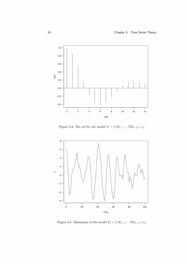
The autocorrelation function for a given model can be computed using theARMAacf function. The acf for the model above can be computed and plottedas follows.
> plot(0:14, ARMAacf(ar=c(1.5,-.75), lag=14), type="h",xlab = "Lag", ylab = "ACF")
> abline(h = 0)
The result is shown in figure 3.4.Finally, it may be useful to simulate a time series of a given form. We can
create a time series from the model Yt = 1.5Yt−1− .75Yt−2 + εt and plot it withthe following statements.
> x = arima.sim(model = list(ar=c(1.5,-.75)), n = 100)> plot(x)
The result is shown in figure 3.5. Note that there is evidence that the seriescontains a quasi-periodic component with period about 12, as suggested by theautocorrelation function.
28 Chapter 3. Time Series Theory
0 2 4 6 8 10 12 14
−0.4
−0.2
0.0
0.2
0.4
0.6
0.8
1.0
Lag
AC
F
Figure 3.4: The acf for the model Yt = 1.5Yt−1 − .75Yt−2 + εt.
Time
x
0 20 40 60 80 100
−6
−4
−2
0
2
4
6
8
Figure 3.5: Simulation of the model Yt = 1.5Yt−1 − .75Yt−2 + εt.

3.6. Moving Average Series 29
3.6 Moving Average Series
A time series {Yt} which satisfies
Yt = εt + θ1εt−1 + · · ·+ θqεt−q (3.9)
(with {εt} white noise) is said to be a moving average process of order q orMA(q) process. No additional conditions are required to ensure stationarity.
The autocovariance function for the MA(q) process is
γ(u) =
(1 + θ21 + · · ·+ θ2q)σ2 u = 0(θu + θ1θu+1 + · · ·+ θq−uθq)σ2 u = 1, . . . , q0 otherwise.
which says there is only a finite span of dependence on the series.Note that it is easy to distinguish MA and AR series by the behaviour of
their autocorrelation functions. The acf for MA series “cuts off” sharply whilethat for an AR series decays exponentially (with a possible sinusoidal ripplesuperimposed).
3.6.1 The MA(1) Series
The MA(1) series is defined by
Yt = εt + θεt−1. (3.10)
It has autocovariance function
γ(u) =
(1 + θ2)σ2 u = 0θσ2 u = 10 otherwise.
and autocorrelation function
ρ(u) =
θ
1 + θ2for u = 1,
0 otherwise.(3.11)
3.6.2 Invertibility
If we replace θ by 1/θ and σ2 by θσ2 the autocorrelation function given by 3.11is unchanged. There are thus two sets of parameter values which can explainthe structure of the series.
For the general process defined by equation 3.9, there is a similar identifia-bility problem. The problem can be resolved by requiring that the operator
1 + θ1L+ · · ·+ θqLq
be invertible – i.e. that all roots of the polynomial
1 + θ1z + · · ·+ θqzq
lie outside the unit circle.

30 Chapter 3. Time Series Theory
0 2 4 6 8 10 12 14
0.0
0.2
0.4
0.6
0.8
1.0
Lag
AC
F
Figure 3.6: The acf for the model Yt = εt + .9εt−1.
3.6.3 Computation
The function polyroot can be used to check invertibility for MA models. Re-member that the invertibility requirement is only so that each MA model is onlydefined by one set of parameters.
The function ARMAacf can be used to compute the acf for MA series. Forexample, the acf of the model
Yt = εt + 0.9εt−1
can be computed and plotted as follows.
> plot(0:14, ARMAacf(ma=.9, lag=14), type="h",xlab = "Lag", ylab = "ACF")
> abline(h = 0)
The result is shown in figure 3.6.A simulation of the series can be computed and plotted as follows.
> x = arima.sim(model = list(ma=.9), n = 100)> plot(x)
The result of the simulation is shown in figure 3.7.
3.7 Autoregressive Moving Average Series
Definition 3.7.1 If a series satisfies
Yt = φ1Yt−1 + · · ·+ φpYt−p + εt + θ1εt−1 + · · ·+ θqεt−q (3.12)

3.7. Autoregressive Moving Average Series 31
Time
x
0 20 40 60 80 100
−3
−2
−1
0
1
2
3
Figure 3.7: Simulation of the model Yt = εt + .9εt−1.
(with {εt} white noise), it is called an autoregressive-moving average series oforder (p, q), or an ARMA(p, q) series.
An ARMA(p, q) series is stationary if the roots of the polynomial
1− φ1z − · · · − φpzp
lie outside the unit circle.
3.7.1 The ARMA(1,1) Series
The ARMA(1,1) series is defined by
Yt = φYt−1 + εt + θεt−1. (3.13)
To derive the autocovariance function for Yt, note that
E(εtYt) = E[εt(φYt−1 + εt + θεt−1)]
= σ2ε
and
E(εt−1Yt) = E[εt−1(φYt−1 + εt + θεt−1)]
= φσ2ε + θσ2
ε
= (φ+ θ)σ2ε .

32 Chapter 3. Time Series Theory
Multiplying equation 3.13 by Yt−u and taking expectation yields:
γ(u) =
φγ(1) + (1 + θ(φ+ θ))σ2
ε u = 0
φγ(0) + θσ2ε u = 1
φγ(u− 1) u ≥ 2
Solving the first two equations produces
γ(0) =(1 + 2θφ+ θ2)
1− φ2σ2
ε =(1 + 2θφ+ θ2)
1− φ2σ2
ε
and using the last recursively shows
γ(u) =(1 + θφ)(φ+ θ)
1− φ2φu−1σ2
ε for u ≥ 1.
The autocorrelation function can then be computed as
ρ(u) =(1 + θφ)(φ+ θ)(1 + 2θφ+ θ2)
φu−1 for u ≥ 1.
The pattern here is similar to that for AR(1), except for the first term.
3.7.2 The ARMA(p,q) Model
It is possible to make general statements about the behaviour of general ARMA(p,q)series. When values are more than q time units apart, the memory of the moving-average part of the series is lost. The functions γ(u) and ρ(u) will then behavevery similarly to those for the AR(p) series
Yt = φ1Yt−1 + · · ·+ φpYt−p + εt
for large u, but the first few terms will exhibit additional structure.
3.7.3 Computation
Stationarity can be checked by examining the roots of the characteristic poly-nomial of the AR operator and model parameterisation can be checked by ex-amining the roots of the characteristic polynomial of the MA operator. Bothchecks can be carried out with polyroot.
The autocorrelation function for an ARMA series can be computed withARMAacf. For the model
Yt = −.5Yt−1 + εt + .3εt−1
this can be done as follows
> plot(0:14, ARMAacf(ar=-.5, ma=.3, lag=14), type="h",xlab = "Lag", ylab = "ACF")
> abline(h = 0)
and produces the result shown in figure 3.8.Simulation can be carried out using arma.sim
> x = arima.sim(model = list(ar=-.5,ma=.3), n = 100)> plot(x)
producing the result in figure 3.9.

3.7. Autoregressive Moving Average Series 33
0 2 4 6 8 10 12 14
−0.2
0.0
0.2
0.4
0.6
0.8
1.0
Lag
AC
F
Figure 3.8: The acf for the model Yt = −.5Yt−1 + εt + .3εt−1.
Time
x
0 20 40 60 80 100
−2
−1
0
1
2
Figure 3.9: Simulation of the model Yt = −.5Yt−1 + εt + .3εt−1.

34 Chapter 3. Time Series Theory
3.7.4 Common Factors
If the AR and MA operators in an ARMA(p, q) model possess common factors,then the model is over-parameterised. By dividing through by the commonfactors we can obtain a simpler model giving and identical description of theseries. It is important to recognise common factors in an ARMA model becausethey will produce numerical problems in model fitting.
3.8 The Partial Autocorrelation Function
The autocorrelation function of an MA series exhibits different behaviour fromthat of AR and general ARMA series. The acf of an MA series cuts of sharplywhereas those for AR and ARMA series exhibit exponential decay (with possi-ble sinusoidal behaviour superimposed). This makes it possible to identify anARMA series as being a purely MA one just by plotting its autocorrelation func-tion. The partial autocorrelation function provides a similar way of identifyinga series as a purely AR one.
Given a stretch of time series values
. . . , Yt−u, Yt−u+1, . . . , Yt−1, Yt, . . .
the partial correlation of Yt and Yt−u is the correlation between these randomvariables which is not conveyed through the intervening values.
If the Y values are normally distributed, the partial autocorrelation betweenYt and Yt−u can be defined as
φ(u) = cor(Yt, Yt−u|Yt−1, . . . , Yt−u+1).
A more general approach is based on regression theory. Consider predictingYt based on Yt−1, . . . , Yt−u+1. The prediction is
Yt = β1Yt−1 + β2Yt−2 · · · , βu−1Yt−u+1
with the βs chosen to minimise
E(Yt − Yt)2.
It is also possible to “think backwards in time” and consider predicting Yt−u
with the same set of predictors. The best predictor will be
Yi−u = β1Yt−u+1 + β2Yt−u+2 · · · , βu−1Yt−1.
(The coefficients are the same because the correlation structure is the samewhether the series is run forwards or backwards in time.
The partial correlation function at lag u is the correlation between the pre-diction errors.
φ(u) = cor(Yt − Yt, Yt−u − Yt−u)
By convention we take φ(1) = ρ(1).
3.8. The Partial Autocorrelation Function 35
It is quite straightforward to compute the value of φ(2). Using the resultsof section 2.4.1, the best predictor of Yt based on Yt−1 is just ρ(1)Yt−1. Thus
cov(Yt − ρ(1)Yt−1, Yt−2 − ρ(1)Yt−1) = σ2Y (ρ(2)− ρ(1)2 − ρ(1)2) + ρ(1)2)
= σ2Y (ρ(2)− ρ(1)2)
and
var(Yt − ρ(1)Yt−1) = σ2Y (1 + ρ(1)2 − 2ρ(1)2)
= σ2Y (1− ρ(1))2
This means that
φ(2) =ρ(2)− ρ(1)2
1− ρ(1)2(3.14)
Example 3.8.1 For the AR(1) series, recall that
ρ(u) = φu (u ≥ 0).
Substituting this into equation 3.14 we find
φ(2) =φ2 − φ2
1− φ2= 0.
Example 3.8.2 For the MA(1) series
ρ(u) =
θ
1 + θ2if u = 1,
0 otherwise.
Substituting this into 3.14 we find
φ(2) =0− (θ/(1 + θ2))2
1− (θ/(1 + θ2))2
=−θ2
(1 + θ2)2 − θ2
=−θ2
1 + θ2 + θ4.
More generally it is possible to show
φ(u) =−θu(1− θ2)1− θ2(u+1)
for u ≥ 0.
For the general AR(p) series, it is possible to show that φ(u) = 0 for allu > p. For such a series, the best predictor of Yt using Yt−1, . . . , Yt−u+1 foru > p is
φ1Yt−1 + · · ·+ φpYt−p.

36 Chapter 3. Time Series Theory
becauseYt − φ1Yt−1 + · · ·+ φpYt−p = εt
and εt is uncorrelated with Yt−1, Yt−2, . . ., so that the “fit” cannot be improved.The prediction error corresponding to the best linear predictor of Yt−u is
based on Yt−1, . . . , Yt−u+1 and so must be uncorrelated with εt. This showsthat φ(u) = 0.
For the general MA(q), it is possible to show that φ(u) decays exponentiallyas u→∞.
3.8.1 Computing the PACF
The definition of the partial autocorrelation function given in the previous sec-tion is conceptually simple, but it makes computations hard. In this sectionwe’ll see that there is an equivalent form which is computationally simple.
Consider the kth order autoregressive prediction of Yk+1
Yk+1 = φk1Yk + · · ·+ φkkY1 (3.15)
obtained by minimising E(Yk+1 − Yk+1)2. We will show that the kth partialautocorrelation values is given by φ(k) = φkk. The proof of this is a geometricone which takes places in the space H generated by the series {Yt}.
We begin by defining the subspace H1 = sp{Y2, . . . , Yk} and associatedprojection PH1 , the subspace H2 = sp{Y1 − PH1Y1} and the subspace Hk =sp{Y1, . . . , Yk}. Any Y ∈ H,
PHkY = PH1Y + PH2Y.
Thus
Yk+1 = PHkYk+1
= PH1Yk+1 + PH2Yk+1
= PH1Yk+1 + a(Y1 − PH1Y1),
wherea = 〈Yk+1, Y1 − PH1Y1〉/‖Y1 − PH1Y1‖2. (3.16)
Rearranging, we find
Yk+1 = PH1(Yk+1 − aY1) + aY1.
The first term on the right must be a linear combination of Y2, . . . , Yk, so com-paring with equation 3.15 we see that a = φkk.
Now, the kth partial correlation is defined as the correlation between theresiduals from the regressions of Yk+1 and Y1 on Y2, . . . , Yk. But this is just
cor(Yk+1 − PH1Yk+1, Y1 − PH1Y1)
= 〈Yk+1 − PH1Yk+1, Y1 − PH1Y1〉/‖Y1 − PH1Y1‖2
= 〈Yk+1, Y1 − PH1Y1〉/‖Y1 − PH1Y1‖2
= a

3.8. The Partial Autocorrelation Function 37
by equation 3.16.A recursive way of computing the regression coefficients in equation 3.15 from
the autocorrelation function was given by Levinson (1947) and Durbin (1960).The Durbin-Levinson algorithm updates the coefficients the from k − 1st ordermodel to those of the kth order model as follows:
φkk =
ρ(k)−k−1∑j=1
φk−1,jρk−j
1−k−1∑j=1
φk−1,jρj
φk,j = φk−1,j − φkkφk−1,k−j j = 1, 2, . . . , k − 1.
3.8.2 Computation
The R function ARMAacf can be used to obtain the partial autocorrelation func-tion associated with a stationary ARMA series. The call to ARMAacf is identicalto its use for obtaining the ordinary autocorrelation function, except it has theadditional argument pacf=TRUE.
The following code computes and plots the partial autocorrelation functionfor the ARMA(1,1) model with φ = −.5 and θ = .3.
> plot(1:14, ARMAacf(ar=-.5, ma=.3, lag=14, pacf=TRUE),type="h", xlab = "Lag", ylab = "ACF")
> abline(h = 0)
The resulting plot is shown in figure 3.10.

38 Chapter 3. Time Series Theory
2 4 6 8 10 12 14
−0.20
−0.15
−0.10
−0.05
0.00
0.05
Lag
AC
F
Figure 3.10: The partial acf for the model Yt = −.5Yt−1 + εt + .3εt−1.
Chapter 4
Identifying Time SeriesModels
4.1 ACF Estimation
We have seen that it is possible to distinguish between AR, MA and ARMAmodels by the behaviour of their acf and pacf functions. In practise, we don’tknow these functions and so we must estimate them.
Given a stretch of data Y1, . . . , YT , the usual estimate of the autocovariancefunction is
γ(u) =1T
T−u∑t=1
(Yt+u − Y )(Yt − Y )
Note that this estimator is biased — an unbiased estimator would have adivisor of T − u in place of T . There are two reasons for using this estimator.
The first of these reasons is that it produces a γ(u) which is positive definite.This means that for any constants c1, . . . , ck,
k∑u=1
k∑v=1
cucvγ(u− v) ≥ 0.
This ensures that our estimate of the variance ofk∑
u=1
cuXt−u
will be non-negative, something which might not be the case for the unbiasedestimate.
The second reason is that for many time series γ(u) → 0 as u → ∞. Forsuch time series, the biased estimate can have lower mean-squared error.
The estimate of ρ(u) based on γ(u) is
r(u) =γ(u)γ(0)
=∑
t(Yt+u − Y )(Yt − Y )∑t(Yt − Y )2
(Again, this can have better mean-squared error properties than the estimatebased on the unbiased estimate of γ(u).)
39

40 Chapter 4. Identifying Time Series Models
In order to say whether an observed correlation is significantly different fromzero, we need some distribution theory. Like most time series results, the theoryhere is asymptotic (as T →∞). The original results in this area were obtainedby Bartlett in 1947. We will look at results due to T. W. Anderson in 1971.
Suppose that
Yt = µ+∞∑
u=0
ψuεt−u
with the εt independent and identically distributed with zero mean and non-zerovariance. Suppose that
∞∑u=0
|ψu| <∞ and∞∑
u=0
u|ψu|2 <∞.
(This is true for all stationary ARMA series). The last condition can be replacedby the requirement that the {Yt} values have a finite fourth moment.
Under these conditions, for any fixed m, the joint distribution of√T (r(1)− ρ(1)),
√T (r(2)− ρ(2)), . . .
√T (r(m)− ρ(m))
is asymptotically normal with zero means and covariances
cuv =∞∑
t=0
(ρ(t+ u)ρ(t+ v) + ρ(t− u)ρ(t+ v)
− 2ρ(u)ρ(t)ρ(t+ v)− 2ρ(v)ρ(t)ρ(t+ u) (4.1)
+ 2ρ(u)ρ(v)ρ(t)2).
I.e. for large T
r(u) ≈ N(0, cuu/T ) cor(r(u), r(v)
)≈ cuv√
cuucvv.
Notice that var r(u) ↓ 0 but that the correlations stay approximately constant.Equation 4.1 is clearly not easy to interpret in general. Let’s examine some
special cases.
Example 4.1.1 White Noise.The theory applies to the case that the Yt are i.i.d.
var r(u) ≈ 1T
cor(r(u), r(v)
)≈ 0
Example 4.1.2 The AR(1) Series.In this case ρ(u) = φu for u > 0. After a good deal of algebra (summinggeometric series) one finds:
var r(u) ≈ 1T
((1 + φ2)(1− φ2u)
1− φ2− 2uφ2u
).
In particular, for u = 1,
var r(1) ≈ 1− φ2
T.

4.1. ACF Estimation 41
Table 4.1: Large Sample Results for rk for an AR(1) Model.
φ√
var r(1)√
var r(2) cor(r(1), r(2)
) √var r(10)
0.9 0.44/√T 0.807/
√T 0.97 2.44/
√T
0.7 0.71/√T 1.12/
√T 0.89 1.70/
√T
0.5 0.87/√T 1.15/
√T 0.76 1.29/
√T
0.3 0.95/√T 1.08/
√T 0.53 1.09/
√T
0.1 0.99/√T 1.01/
√T 0.20 1.01/
√T
Notice that the closer φ is to ±1, the more accurate the estimate becomes.As u→∞, φ2u → 0. In that case
var r(u) ≈ 1T
(1 + φ2
1− φ2
).
For values of φ close to ±1 this produces large variances for the r(u).For 0 < u 6 v (after much algebra),
cuv =(φv−1 − φv+u)(1 + φ2)
1− φ2+ (v − u)φv−u − (v + u)φv+u.
In particular,
cor(r(1), r(2)
)≈ 2φ
(1− φ2
1 + 2φ2 − 3φ4
)1/2
Using these formulae it is possible to produce the results in table 4.1.
Example 4.1.3 The MA(1) SeriesFor the MA(1) series it is straightforward to show that
c11 = 1− 3ρ(1)2 + 4ρ(1)4
cuu = 1− 2ρ(1)2 u > 1
c12 = 2ρ(1)(1− ρ(1)2)
Using these results it is easy to produce the results in table 4.2.
Example 4.1.4 The General MA(q) SeriesIn the case of the general MA(q) series it is easy to see that
cuu = 1 + 2q∑
v=1
ρ(v)2, for u > q,
and hence that
var r(u) =1T
(1 + 2
q∑v=1
ρ(v)2), for u > q.

42 Chapter 4. Identifying Time Series Models
Table 4.2: Large Sample Results for rk for an MA(1) Model.
θ√
var r(1)√
var r(k) (k > 1) cor(r(1), r(2)
)0.9 0.71/
√T 1.22/
√T 0.86
0.7 0.73/√T 1.20/
√T 0.84
0.5 0.79/√T 1.15/
√T 0.74
0.4 0.84/√T 1.11/
√T 0.65
Notes
1. In practise we don’t know the parameters of the model generating the datawe might have. We can still estimate the variances and covariances of ther(u) by substituting estimates of ρ(u) into the formulae above.
2. Note that there can be quite large correlations between the r(u) values socaution must be used when examining plots of r(u).
4.2 PACF Estimation
In section 3.8.1 we saw that the theoretical pacf can be computed by solvingthe Durbin-Levinson recursion
φkk =
ρ(k)−k−1∑j=1
φk−1,jρ(k − j)
1−k−1∑j=1
φk−1,jρ(j)
φk,j = φk−1,j − φkkφk−1,k−j j = 1, 2, . . . , k − 1.
and setting φ(u) = φuu.In practice, the estimated autocorrelation function is used in place of the
theoretical autocorrelation function to generate estimates of the partial auto-correlation function.
To decide whether partial autocorrelation values are significantly differentfrom zero, we can use a (1949) result of Quenouille which states that if the trueunderlying model is AR(p), then the estimated partial autocorrelations at lagsgreater than p are approximately independently normal with means equal tozero and variance 1/T . Thus ±2/
√T can be used as critical limits on φ(u) for
u > p to test the hypothesis of an AR(p) model.

4.3. System Identification 43
Time
Diff
eren
ce In
Yie
ld
1962 1964 1966 1968 1970 1972 1974
0.4
0.6
0.8
1.0
1.2
1.4
1.6
Figure 4.1: Monthly differences between the yield on mortgages andgovernment loans in the Netherlands, January 1961 to March 1974.
4.3 System Identification
Given a set of observations Y1, . . . , YT we will need to decide what the appro-priate model might be. The estimated acf and pacf are the tools which can beused to do this. If the acf exhibits slow decay and the pacf cuts off sharply afterlag p, we would identify the series as AR(p). If the pacf shows slow decay andthe acf show a sharp cutoff after lag q, we would identify the series as beingMA(q). If both the acf and pacf show slow decay we would identify the seriesas being mixed ARMA. In this case the orders of the AR and MA parts are notclear, but it is reasonable to first try ARMA(1,1) and move on to higher ordermodels if the fit of this model is not good.
Example 4.3.1 Interest Yields
Figure 4.1 shows a plot of the Monthly differences between the yield on mort-gages and government loans in the Netherlands, January 1961 to March 1974.The series appears stationary, so we can attempt to use the acf and pacf todecide whether an AR, MA or ARMA model might be appropriate.
Figures 4.2 and 4.3 show the estimated acf and pacf functions for the yieldseries. The horizontal lines in the plots are drawn at the y values ±1.96/
√159
(the series has 159 values). These provide 95% confidence limits for what canbe expected under the hypothesis of white noise. Note that these limits arepoint-wise so that we would expect to see roughly 5% of the values lying outsidethe limits.
The acf plot shows evidence of slow decay, while the pacf plot shows a“sharp

44 Chapter 4. Identifying Time Series Models
0.0 0.5 1.0 1.5
−0.2
0.0
0.2
0.4
0.6
0.8
1.0
Lag
AC
F
Figure 4.2: The acf for the yield data.
0.5 1.0 1.5
0.0
0.2
0.4
0.6
0.8
Lag
Par
tial A
CF
Figure 4.3: The pacf for the yield data.

4.4. Model Generalisation 45
Time
Yie
ld
0 10 20 30 40 50 60 70
30
40
50
60
70
80
Figure 4.4: Yields from a chemical process (from Box and Jenkins).
cutoff” after lag 1. On the basis of these two plots we might hypothesise thatan AR(1) model was an appropriate description of the data.
Example 4.3.2 Box and Jenkins Chemical Yields
Figure 4.4 shows an example from the classic time series text by Box and Jenk-ins. This series contains consecutive yields recorded from a chemical process.Again, the series is apparently stationary so that we can consider identifying anappropriate model on the basis of the acf and pacf.
Again, the acf seems to show slow decay, this time with alternating signs.The pacf shows sudden cutoff after lag 1, suggesting that again an AR(1) modelmight be appropriate.
4.4 Model Generalisation
ARMA series provide a flexible class of models for stationary mean-zero series,with AR and MA series being special cases.
Unfortunately, many series are clearly not in this general class for models.It is worthwhile looking at some generalisation of this class.
4.4.1 Non-Zero Means
When a series {Yt} has a non-zero mean µ, the mean can be subtracted and thedeviations from the mean modeled as an ARMA series.
Yt − µ = φ1(Yt−1 − µ) + · · ·+ φp(Yt−p − µ) + εt + θ1εt−1 + · · ·+ θqεt−q

46 Chapter 4. Identifying Time Series Models
0 5 10 15
−0.4
−0.2
0.0
0.2
0.4
0.6
0.8
1.0
Lag
AC
F
Figure 4.5: The acf for the chemical process data.
5 10 15
−0.4
−0.3
−0.2
−0.1
0.0
0.1
0.2
Lag
Par
tial A
CF
Figure 4.6: The pacf for the chemical process data.

4.4. Model Generalisation 47
Alternatively, the model can be adjusted by introducing a constant directly.
Yt = φ1Yt−1 + · · ·+ φpYt−p + θ0 + εt + θ1εt−1 + · · ·+ θqεt−q
The two characterisations are connected by
θ0 = µ− µ(φ1 + · · ·+ φp)
so thatµ =
θ01− φ1 − · · · − φp
orθ0 = µ(1− φ1 − · · · − φp).
4.4.2 Deterministic Trends
Consider the modelYt = f(t) + Zt,
where Zt is a stationary ARMA series and f(t) is a deterministic function of t.Considering Yt− f(t) reduces Yt to an ARMA series. (If f(t) contains unknownparameters we can estimate them.)
4.4.3 Models With Non-stationary AR Components
We’ve seen that any AR model with characteristic equation roots outside theunit circle will be non-stationary.
Example 4.4.1 Random WalksA random walk is defined by the equation
Yt = Yt−1 + εt
where {εt} is a series of uncorrelated (perhaps independent) random variables.In operator form this equation is
(1− L)Yt = εt.
The equation 1− z = 0 has a root at 1 so that Yt is non-stationary.
Example 4.4.2 Integrated Moving AveragesConsider the model
Yt = Yt−1 + εt + θεt−1.
This is similar to an ARMA(1,1) model, but again it is non-stationary.
Both these models can be transformed to stationarity by differencing —transforming to ∇Yt = Yt − Yt−1. In the first example we have,
∇Yt = εt,
which is the white noise model. In the second we have,
∇Yt = εt + θεt−1,
which is the MA(1) model.

48 Chapter 4. Identifying Time Series Models
4.4.4 The Effect of Differencing
Suppose that Yt has a linear trend
Yt = β0 + β1t+ Zt
where Zt is stationary with E(Zt) = 0.
∇Yt = β1 +∇Zt
Differencing has removed the trend. Now suppose that {Yt} has a deterministicquadratic trend
Yt = β0 + β1t+ β2t2 + Zt
then
∇Yt = (β0 + β1t+ β2t2)− (β0 + β1(t− 1) + β2(t− 1)2) +∇Zt
= β1 + β2(t2 − (t2 − 2t+ 1)) +∇Zt
= (β1 − β2) + 2β2t+∇Zt
= linear trend + stationary.
Differencing again produces
∇2Yt = 2β2 +∇2Zt.
In general, a polynomial trend of order k can be eliminated by differencing ktimes.
Now let’s consider the case of a “stochastic trend.” Suppose that
Yt = Mt + εt
where Mt is a random process which changes slowly over time. In particular,we can assume that Mt is generated by a random walk model.
Mt = Mt−1 + ηt
with ηt independent of εt. Then
∇Yt = ηt + εt − εt−1.
∇Yt is stationary and has an autocorrelation function like that of an MA(1)series.
ρ(1) =−1
2 + (ση/σε)2
More generally, “higher order” stochastic trend models can be reduced to sta-tionarity by repeated differencing.

4.5. ARIMA Models 49
4.5 ARIMA Models
If Wt = ∇dYt is an ARMA(p,q) series than Yt is said to be an integrated autore-gressive moving-average (p, d, q) series, denoted ARIMA(p,d,q). If we write
φ(L) = 1− φ1L− · · · − φpLp
andθ(L) = 1 + θ1L+ · · ·+ θqL
q
then we can write down the operator formulation
φ(L)∇dYt = θ(L)εt.
Example 4.5.1 The IMA(1,1) Model This model is widely used in businessand economics. It is defined by
Yt = Yt−1 + εt + θεt−1.
Yt can be thought of as a random walk with correlated errors.Notice that
Yt = Yt−1 + εt + θεt−1
= Yt−2 + εt−1 + θεt−2 + εt + θεt−1
= Yt−2 + εt + (1 + θ)εt−1 + θεt−2
...
= Y−m + εt + (1 + θ)εt−1 + · · ·+ (1 + θ)ε−m + θε−m−1
If we assume that Y−m = 0 (i.e. observation started at time −m),
Yt = εt + (1 + θ)εt−1 + · · ·+ (1 + θ)ε−m + θε−m−1
This representation can be used to derive the formulae
var(Yt) =(1 + θ2 + (1 + θ)2(t+m)
)σ2
ε
cor(Yk, Yt−k
)=
1 + θ2 + (1 + θ)2(t+m− k)(var(Yt)var(Yt−k)
)1/2
=
√t+m− k
t+m
≈ 1
for m large and k moderate. (We are considering behaviour after “burn-in.”)This means that we can expect to see very slow decay in the autocorrelationfunction.
The very slow decay of the acf function is characteristic of ARIMA serieswith d > 0. Figures 4.7 and 4.8 show the estimated autocorrelation functionsfrom a simulated random walk and an integrated autoregressive model. Bothfunctions show very slow declines in the acf.

50 Chapter 4. Identifying Time Series Models
0 5 10 15 20
0.0
0.2
0.4
0.6
0.8
1.0
Lag
AC
F
Figure 4.7: The autocorrelation function of the ARIMA(0,1,0) (randomwalk) model.
0 5 10 15 20
0.0
0.2
0.4
0.6
0.8
1.0
Lag
AC
F
Figure 4.8: The autocorrelation function of the ARIMA(1,1,0) modelwith φ1 = .5.

Chapter 5
Fitting and Forecasting
5.1 Model Fitting
Suppose that we have identified a particular ARIMA(p,d,q) model which appearsto describe a given time series. We now need to fit the identified model andassess how well the model fits. Fitting is usually carried out using maximumlikelihood. For a given set of model parameters, we calculate a series of one-step-ahead predictions.
Yk+1 = PHkYk+1
where Hk is the linear space spanned by Y1, . . . , Yk. The predictions are ob-tained in a recursive fashion using a process known as Kalman filtering. Eachprediction results in a prediction error Yk+1 − Yk+1. These are, by construc-tion, uncorrelated. If we add the requirement that the {Yt} series is normallydistributed, the prediction errors are independent normal random variables andthis can be used as the basis for computing the likelihood.
The parameters which need to be estimated are the AR coefficients φ1, . . . , φp,the MA coefficients θ1, . . . , θq and a constant term (either µ or θ0 as outlinedin section 4.4.1). Applying maximum-likelihood produces both estimates andstandard errors.
5.1.1 Computations
Given a time series y in R, we can fit an ARMA(p,d,q) model to the series asfollows
> z = arima(y, order=c(p, d, q))
The estimation results can be inspected by printing them.
Example 5.1.1 U.S. Unemployment RatesFigure 5.1 shows a plot of the seasonally adjusted quarterly United States un-employment rates from the first quarter of 1948 to the first quarter of 1978.If the data is stored as a time series in the R data set unemp, the plot can beproduced with the command
> plot(unemp)
51

52 Chapter 5. Fitting and Forecasting
Time
unem
p
1950 1955 1960 1965 1970 1975
3
4
5
6
7
8
9
Figure 5.1: United States quarterly unemployment rates (seasonallyadjusted).
Neither the original series nor the presence of very slow decay in the acf(figure 5.2) indicate strongly that differencing is required so we will leave theseries undifferenced and attempt to find an appropriate ARMA model.
The acf and pacf functions for the series can be computed and plotted withthe following commands
> acf(unemp)
> pacf(unemp)
The resulting plots (figures 5.2 and 5.3) show the strong signature of an AR(2)series (slow decay of the acf and sharp cutoff of the pacf after two lags.)
With the series identified we can go about estimating the unknown param-eters. We do this with the arima function in R.
> z = arima(unemp, order=c(2, 0, 0))
> z
Call:arima(x = unemp, order = c(2, 0, 0))
Coefficients:ar1 ar2 intercept
1.5499 -0.6472 5.0815s.e. 0.0681 0.0686 0.3269
sigma^2 estimated as 0.1276: log likelihood = -48.76, aic = 105.53
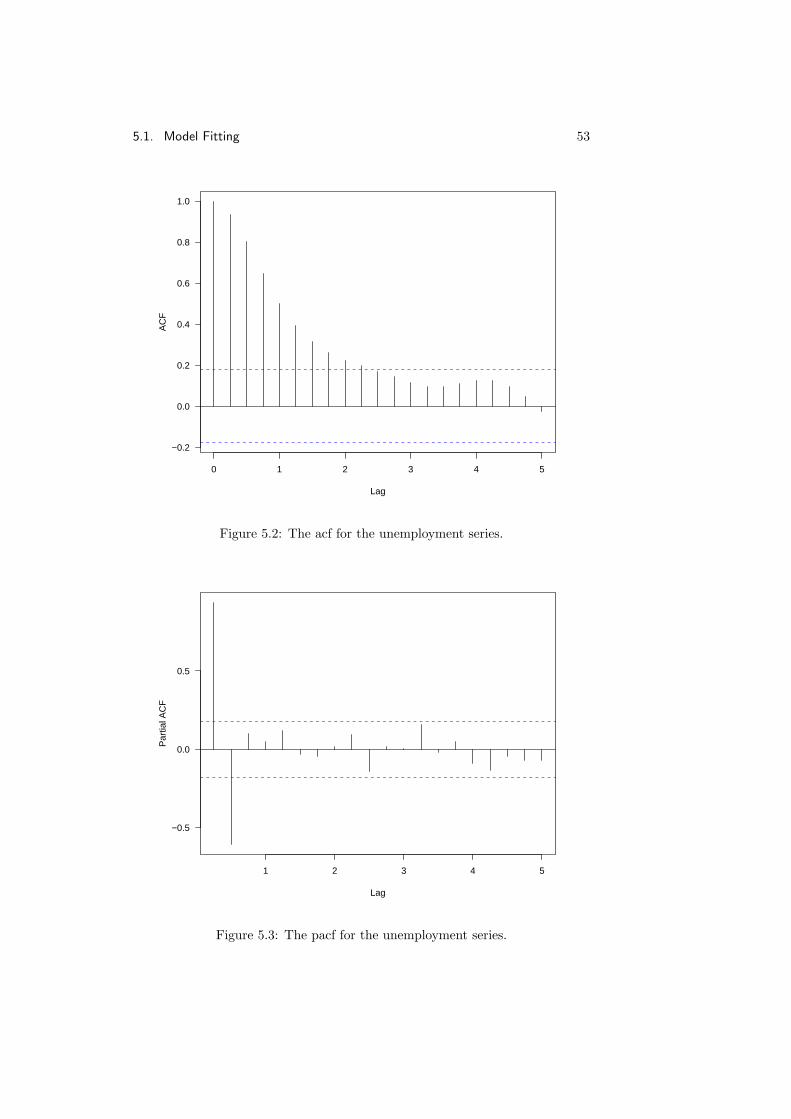
5.1. Model Fitting 53
0 1 2 3 4 5
−0.2
0.0
0.2
0.4
0.6
0.8
1.0
Lag
AC
F
Figure 5.2: The acf for the unemployment series.
1 2 3 4 5
−0.5
0.0
0.5
Lag
Par
tial A
CF
Figure 5.3: The pacf for the unemployment series.

54 Chapter 5. Fitting and Forecasting
The fitted model in this case is
Yt = 5.0815 + 1.5499 Yt−1 − 0.6472 Yt−2 + εt
where εt has an estimated variance of 0.1276.
Example 5.1.2 Railroad Bond YieldsFigure 5.4 shows a plot of the monthly yields on AA rated railroad bonds (as apercentage times 100). With the data values stored in the R variable rrbonds,the plot was produced with the command
> plot(rrbonds, ylab = "Bond Yields")
In this case it is clear that the series is non-stationary and we need to trans-form to stationarity by taking differences. The series can be differenced and theresult plotted as follows
> rrdiffs = diff(rrbonds)
> plot(rrdiffs, ylab = "Differenced Yields")
Figure 5.5 shows a plot of the differenced series and it is clear from this plotthat the assumption of stationarity is much more reasonable. To confirm this,and to suggest possible models we need to examine the acf and pacf functions.These are shown in figures 5.6 and 5.7.
The model signature here is less certain than that of the previous example.A possible interpretation is that the acf is showing rapid decay and the pacfis showing sharp cutoff after one lag. This suggests that original series can bemodelled as an ARIMA(1,1,0) series.
The estimation of parameters can be carried out for this model as follows
> z = arima(rrbonds,order=c(1,1,0))
> z
Call:arima(x = rrbonds, order = c(1, 1, 0))
Coefficients:ar1
0.4778s.e. 0.0865
sigma^2 estimated as 84.46: log likelihood = -367.47, aic = 738.94
The fitted model in this case is
∇Yt = 0.4778 ∇Yt + εt.
with εt having an estimated variance of 84.46.
5.2 Assessing Quality of Fit
Once a model has been fitted to a set of data it is always important to assesshow well the model fits. This is because the inferences we make depend crucially

5.2. Assessing Quality of Fit 55
Time
Bon
d Y
ield
s
1968 1970 1972 1974 1976
650
700
750
800
850
900
Figure 5.4: Monthly AA railroad bond yields (%× 100).
Time
Diff
eren
ced
Yie
lds
1968 1970 1972 1974 1976
−20
−10
0
10
20
30
Figure 5.5: Differenced monthly AA railroad bond yields.

56 Chapter 5. Fitting and Forecasting
0.0 0.5 1.0 1.5
−0.2
0.0
0.2
0.4
0.6
0.8
1.0
Lag
AC
F
Figure 5.6: The ACF for the differenced monthly AA railroad bondyields.
0.5 1.0 1.5
−0.2
−0.1
0.0
0.1
0.2
0.3
0.4
Lag
Par
tial A
CF
Figure 5.7: The PACF for the differenced monthly AA railroad bondyields.

5.2. Assessing Quality of Fit 57
on the appropriateness of the fitted model. The usual way of assessing goodnessof fit is through the examination of residuals.
In the case of autoregressive models it is easy to see how residuals might bedefined. In the case of the AR(p) model
Yt = φ1Yt−1 + · · ·+ φpYt−p + εt
it is clear that we can take the residuals to be
εt = Yt − φ1Yt−1 + · · ·+ φpYt−p
In the general ARMA case
Yt = φ1Yt−1 + · · ·+ φpYt−p + εt + θ1εt−1 + · · ·+ θqεt−q
orφ(L) = θ(L)εt−q
we must first transform to autoregressive form by inverting the MA operator.
θ(L)−1φ(L) = εt
or
Yt =∞∑
u=1
πuYt−u + εt.
The residuals can then be defined as
εt = Yt −∞∑
u=1
πuYt−u.
This is a useful theoretical approach, but in practise the residuals are ob-tained as a byproduct of the computation of the likelihood (they are the predic-tion errors from the one-step ahead forecasts). If the ARMA model is correct(and the series is normally distributed) then the residuals are approximatelyindependent normal random variables with mean zero and variance σ2
ε .A simple diagnostic is to simply plot the residuals and to see whether they
appear to be a white noise series. In the case of the US unemployment serieswe can do this as follows
> z = arima(unemp, order=c(2, 0, 0))
> plot(resid(z))
The results are shown in figure 5.8.It is also possible to carry out tests of normality on the residuals. This can
be done by simply producing a histogram of the residuals or by performing anormal quantile-quantile plot. This can be done as follows:
> hist(resid(z))
> qqnorm(resid(z))
A simple check of heteroscedasticity can be carried out by plotting the resid-uals against the fitted values. This is done with the following command:
> plot(unemp - resid(z), resid(z),
+ xy.lines = FALSE, xy.labels = FALSE)
None of these plots indicate that there is any problem with the fit of the model.

58 Chapter 5. Fitting and Forecasting
Time
resi
d(z)
1950 1955 1960 1965 1970 1975
−0.5
0.0
0.5
1.0
Figure 5.8: Residuals from the unemployment data.
5.3 Residual Correlations
It is tempting to examine the quality of model fit by seeing whether the residualsform an uncorrelated sequence. One might for example plot the estimated acfof the residuals and look for lags where the correlations exceed ±2/
√T . Unfor-
tunately, while these limits are approximately correct for large lags, for smalllags they overstate the variability of the estimated correlations. This should beno surprise, the effect of model-fitting is to remove as much of the correlationpresent in the series as possible. The correlations between the residuals shouldbe closer to zero than for a non-fitted series.
In addition to checking whether there are large individual correlations presentin a time series, it can be useful to pool information from successive correlationsto see whether there is significant correlation left in the residuals.
One test statistic in common use is the modified Box-Pierce (or Ljung-Box-Pierce) statistic
Q∗ = T (T + 2)K∑
k=1
r2kT − k
.
If the true underlying model is ARMA(p,q), the distribution of Q∗ is approxi-mately χ2
K−p−q.In R, the modified Box-Pierce statistic (and an older variant) can be com-
puted with the function Box.test (you should specify type="Ljung"). Analternative is to use the function tsdiag which plots the (standardised) residu-als, the acf of the residuals and the modified Box-Pierce statistic for a varietyof values of K. In the case of the US unemployment series, an appropriate

5.4. Forecasting 59
command would be
> tsdiag(z)
This produces the plot shown in figure 5.9. The first panel of the plot shows the(standardised) residuals from the model fit. The residuals look reasonably ran-dom but during the period from 1965 to 1970 there is a sequence of values whichare all negative. This indicates that there may be problems with the model fit.The second panel shows the autocorrelation function for the residuals. One ofthe correlations (that at a lag of 7 quarters) lies outside the two standard errorbounds about zero. Since we would expect one in twenty of the estimated cor-relations to exceed these bounds this does not provide evidence for a significantcorrelation. The third panel shows p-values for the Ljung-Box statistics at lagsfrom one quarter to ten quarters. There is no evidence of significant correlationin this plot.
Overall, there is some evidence of lack of fit, but there is no obvious wayof fixing the problem. Because of this we will move on to making forecasts forthe series, but keep in mind that we need to be cautious in making use of theseforecasts.
5.4 Forecasting
Once we have decided on an appropriate time-series model, estimated its un-known parameters and established that the model fits well, we can turn to theproblem of forecasting future values of the series.
The autoregressive representation
Yt =∞∑
u=1
πuYt−u + εt.
suggests predicting the next observation beyond Y1, . . . , YT using
YT+1 =∞∑
u=1
πuYT+1−u.
where the πu are obtained by substituting the estimated parameters in place ofthe theoretical ones.
Once a forecast is obtained for YT+1 we can use it to obtain a forecast forYT+2 and then use these two forcasts to generate a forecast for YT+3. Theprocess can be continued to obtain forecasts out to any point in the future.Because uncertainty increases as we predict further and further from the datawe have, we can expect the standard errors associated with our predictions toincrease.
In practise, forecasts are generated by the same Kalman filter algorithm usedto compute the likelihood used for parameter estimation.
5.4.1 Computation
Once a model has been fitted using arima, the function predict can be used toobtain forecasts. In the case of the US unemployment series we could obtain 10future forecasts as follows:

60 Chapter 5. Fitting and Forecasting
Standardized Residuals
Time
1950 1955 1960 1965 1970 1975
−2
−1
0
1
2
3
0 1 2 3 4 5
−0.2
0.0
0.2
0.4
0.6
0.8
1.0
Lag
AC
F
ACF of Residuals
●
●
●
●
●
●
●●
● ●
2 4 6 8 10
0.0
0.2
0.4
0.6
0.8
1.0
p values for Ljung−Box statistic
lag
p va
lue
Figure 5.9: Residual diagnostics for the US unemployment series.

5.5. Seasonal Models 61
> z = arima(unemp,order=c(2, 0, 0))
> p = predict(z, n.ahead = 10)
The predictions can be viewed with the command
> p$pred
Qtr1 Qtr2 Qtr3 Qtr41978 5.812919 5.491268 5.2432531979 5.067017 4.954379 4.893856 4.8729471980 4.879708 4.903719 4.936557
and their standard errors with
> p$se
Qtr1 Qtr2 Qtr3 Qtr41978 0.3572328 0.6589087 0.90950401979 1.0969935 1.2248696 1.3040856 1.34794991980 1.3689669 1.3771201 1.3792859
It can be useful to plot the forecasts on the same graph as the original timeseries. This a relatively complex task, and would probably be worth packagingup as an R function. Here is how 20 forecasts for the unemp series and theirstandard errors can be plotted
> p = predict(z, n.ahead = 20)
> xlim = range(time(unemp), time(p$pred))
> ylim = range(unemp, p$pred - 2 * p$se, p$pred + 2 * p$se)
> plot(unemp, xlim = xlim, ylim = ylim)
> lines(p$pred, lwd=2)
> lines(p$pred - 2 * p$se, lty = "dotted")
> lines(p$pred + 2 * p$se, lty = "dotted")
The result of this appears in figure 5.10.Notice that the standard errors around forecasts widen rapidly and the fore-
casts themselves seem to be tending to a constant value. If we extend theforecast period, this becomes more obvious as shown in figure 5.11. In fact, overthe long term, forecasts for stationary series ultimately converge to the mean ofthe series and the standard errors for the forecasts tend to the standard devia-tion of the series. This means that we can only expect to gain advantage fromthe use of short-term forecasts.
5.5 Seasonal Models
5.5.1 Purely Seasonal Models
Many time series exhibit strong seasonal characteristics. We’ll use s to denotethe seasonal period. For monthly series, s = 12, and for quarterly series s = 4.These are the most common cases, but seasonal patterns can show up in otherplaces (e.g. weekly patterns in daily observations or daily patterns in hourlydata).

62 Chapter 5. Fitting and Forecasting
Time
unem
p
1950 1955 1960 1965 1970 1975 1980
2
3
4
5
6
7
8
9
Figure 5.10: Forecasts for the unemployment data.
Time
1976 1978 1980 1982 1984
2
3
4
5
6
7
8
9
Figure 5.11: Long-term forecasts for the US unemployment series.

5.5. Seasonal Models 63
Seasonal effects can be modelled by including coefficients at lags which aremultiples of the seasonal period. For example, the model
Yt +Φ1Yt−s +Φ2Yt−2s + · · ·+ΦPYt−Ps = εt +Θ1εt−s +Θ2εt−2s + · · ·+Θqεt−Qs
is the seasonal analog of an ARMA model. Caution is required with modelswhich only involve coefficients at multiples of the seasonal period because theyprovide independent models for each of s seasonal sub-series and make no state-ment about the relationship between the series. For example, the model aboveapplies equally well to the case where the seasonal sub-series are identical
Yks+1 = Yks+2 = · · · = Yks+s
as it does to the case where they are independent.
5.5.2 Models with Short-Term and Seasonal Components
In practise, series will have a mixture of both seasonal and short-term dependen-cies. It is possible to consider models for such series by including both seasonaland non-seasonal terms. This can be done directly, but it turns out to be moreuseful to consider a slightly different class of model.
Recall that the general ARMA(p,q) model can be written as
φ(L)Yt = θ(L)εt.
Each of the θ(L) and φ operators can be written as polynomials in L. Thesehave the factorised form
(1 + a1L)(1 + a2L) · · · (1 + apL)Yt = (1 + b1L)(1 + b2L) · · · (1 + bpL)εt.
Non-stationarity can also be handled by introducing additional factors of theform (1−L). This suggests a different way of handling seasonal effects. We cansimply introduce additional factors of the form (1+AL12) into the autoregressiveoperator or (1 +BL12) into the moving average operator.
The operator on each side of the general model is generally written as aproduct of a polynomial in L times a polynomial in Ls. The general ARMAmodel is
Φ(Ls)φ(L)Yt = Θ(Ls)θ(L)εt,
where Φ is a polynomial of degree P , φ is a polynomial of degree p, Θ is apolynomial of order Q and θ is a polynomial of degree q. Such a model isdenoted as ARMA(p, q)× (P,Q)s.
Non-stationarity can be accommodated by introducing additional differenc-ing terms. This produces a seasonal ARIMA model, the most general form ofwhich is
Φ(Ls)φ(L)(1− L)d(1− Ls)DYt = Θ(Ls)θ(L)εt,
which is denoted by ARMA(p, d, q)× (P,D,Q)s.As an example, we’ll consider the monthly average temperatures in Dubuque,
Iowa, from January 1964 to December 1975. Figure 5.12 shows a plot of theseries. It contains a very strong seasonal pattern. The strength of the patternsuggests that we should start by differencing the series at the seasonal lag.

64 Chapter 5. Fitting and Forecasting
Time
tem
pdub
1964 1966 1968 1970 1972 1974 1976
10
20
30
40
50
60
70
Figure 5.12: Monthly average temperatures ◦C in Dubuque, Iowa.
Time
diff(
tem
pdub
, 12)
1966 1968 1970 1972 1974 1976
−10
−5
0
5
10
Figure 5.13: The seasonally differenced Dubuque temperature series.

5.5. Seasonal Models 65
0 1 2 3 4
−0.4
−0.2
0.0
0.2
0.4
0.6
0.8
1.0
Lag
AC
F
Figure 5.14: The acf of the seasonally differenced Dubuque temperatureseries.
Figure 5.13 shows a plot of the seasonally differenced series and 5.14 showsits acf function. Together the plots indicate the differenced series is stationary.To decide on an appropriate model we also need to inspect a plot of the pacf ofthe seasonally differenced series. This is shown in figure 5.15. When taken inconjunction with the structure of the acf, we have clear evidence that a seasonalMA(1) is an appropriate model for the differenced series.
The R function arima can be used to fit the full model, which is ARIMA(0, 0, 0) × (0, 1, 1)12. Assuming that the series has been read into the variabletempdub, the fitting process and display of the results can be carried out asfollows.
> z = arima(tempdub, seas = c(0,1,1))
> z
Call:arima(x = tempdub, seasonal = c(0, 1, 1))
Coefficients:sma1
-1.0000s.e. 0.0967
sigma^2 estimated as 11.69: log likelihood = -364.48,aic = 732.96

66 Chapter 5. Fitting and Forecasting
0 1 2 3 4
−0.3
−0.2
−0.1
0.0
0.1
Lag
Par
tial A
CF
Figure 5.15: The pacf of the seasonally differenced Dubuque tempera-ture series.
Before producing forecasts of the series we need to check the residuals fromthe fitting process to see that they are (close to) white noise. As before, thiscan be done with the tsdiag function.
> tsdiag(z)
As shown by figure 5.16, the model seems to fit well.
5.5.3 A More Complex Example
Figure 5.17 shows a plot of a data set presented by Box and Jenkins in theirclassic time series text. The plot shows the number of international airlinepassengers, recorded monthly. There is clearly a strong seasonal trend presentin the data — the number of passengers peaks during the Northern summer.
There is a clear seasonal effect present in the series, but the size of theseasonal effects seems to be increasing as the level of the series increases. Thenumber of passengers is clearly increasing with time, with the number travellingin July and August always being roughly 50% greater than the number travellingin January and February. This kind of proportional variability suggests that itwould be more appropriate to examine the series on a log scale. Figure 5.18shows the data plotted in this way. On that scale the series shows a consistentlevel of seasonal variation across time. It seems appropriate to analyse this timeseries on the log scale.
The transformed series is clearly nonstationary. This means that we need toconsider differencing. The series appears to contain both an upward trend and a

5.5. Seasonal Models 67
Standardized Residuals
Time
1964 1966 1968 1970 1972 1974 1976
−2
−1
0
1
2
3
0.0 0.5 1.0 1.5
−0.2
0.0
0.2
0.4
0.6
0.8
1.0
Lag
AC
F
ACF of Residuals
●●
●
●
●
●
●
●●
●
2 4 6 8 10
0.0
0.2
0.4
0.6
0.8
1.0
p values for Ljung−Box statistic
lag
p va
lue
Figure 5.16: Residual diagnostics for the Dubuque temperature series.

68 Chapter 5. Fitting and Forecasting
Time
Tho
usan
ds o
f Pas
seng
ers
1950 1952 1954 1956 1958 1960
100
200
300
400
500
600
Figure 5.17: International airline passengers, monthly totals (in thou-sands).
Time
log 1
0 Tho
usan
ds o
f Pas
seng
ers
1950 1952 1954 1956 1958 1960
2.0
2.2
2.4
2.6
2.8
Figure 5.18: The log international airline passenger series.
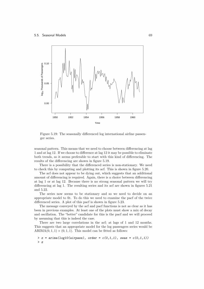
5.5. Seasonal Models 69
Time
log 1
0 Tho
usan
ds o
f Pas
seng
ers
1950 1952 1954 1956 1958 1960
0.00
0.05
0.10
Figure 5.19: The seasonally differenced log international airline passen-ger series.
seasonal pattern. This means that we need to choose between differencing at lag1 and at lag 12. If we choose to difference at lag 12 it may be possible to eliminateboth trends, so it seems preferable to start with this kind of differencing. Theresults of the differencing are shown in figure 5.19.
There is a possibility that the differenced series is non-stationary. We needto check this by computing and plotting its acf. This is shown in figure 5.20.
The acf does not appear to be dying out, which suggests that an additionalamount of differencing is required. Again, there is a choice between differencingat lag 1 or at lag 12. Because there is no strong seasonal pattern we will trydifferencing at lag 1. The resulting series and its acf are shown in figures 5.21and 5.22.
The series now seems to be stationary and so we need to decide on anappropriate model to fit. To do this we need to examine the pacf of the twicedifferenced series. A plot of this pacf is shown in figure 5.23.
The message conveyed by the acf and pacf functions is not as clear as it hasbeen in previous examples. At least one of the plots must show a mix of decayand oscillation. The “better” candidate for this is the pacf and we will proceedby assuming that this is indeed the case.
There are two large correlations in the acf; at lags of 1 and 12 months.This suggests that an appropriate model for the log passengers series would beARIMA(0, 1, 1)× (0, 1, 1). This model can be fitted as follows:
> z = arima(log10(airpass), order = c(0,1,1), seas = c(0,1,1))
> z
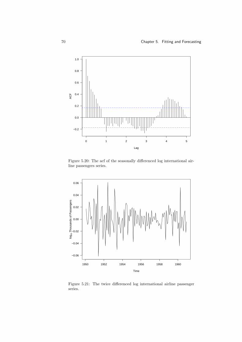
70 Chapter 5. Fitting and Forecasting
0 1 2 3 4 5
−0.2
0.0
0.2
0.4
0.6
0.8
1.0
Lag
AC
F
Figure 5.20: The acf of the seasonally differenced log international air-line passengers series.
Time
log 1
0 Tho
usan
ds o
f Pas
seng
ers
1950 1952 1954 1956 1958 1960
−0.06
−0.04
−0.02
0.00
0.02
0.04
0.06
Figure 5.21: The twice differenced log international airline passengerseries.

5.5. Seasonal Models 71
0 1 2 3 4 5
−0.4
−0.2
0.0
0.2
0.4
0.6
0.8
1.0
Lag
AC
F
Figure 5.22: The acf of the twice differenced log international airlinepassengers series.
0 1 2 3 4 5
−0.3
−0.2
−0.1
0.0
0.1
0.2
Lag
Par
tial A
CF
Figure 5.23: The pacf of the twice differenced log international airlinepassengers series.

72 Chapter 5. Fitting and Forecasting
Call:arima(x = log10(airpass), order = c(0, 1, 1),
seasonal = c(0, 1, 1))
Coefficients:ma1 sma1
-0.4018 -0.5569s.e. 0.0896 0.0731
sigma^2 estimated as 0.0002543: log likelihood = 353.96,aic = -701.92
Both coefficients are highly significant, so we can move onto examining theresiduals with the tsdiag function. The results are shown in figure 5.24 andindicate that the model fits well.
Finally, we can obtain and plot forecasts for the series. These are shown infigure 5.25.

5.5. Seasonal Models 73
Standardized Residuals
Time
1950 1952 1954 1956 1958 1960
−3
−2
−1
0
1
2
3
0.0 0.5 1.0 1.5
−0.2
0.0
0.2
0.4
0.6
0.8
1.0
Lag
AC
F
ACF of Residuals
●
●
●
●
●
●
●
●
●
●
2 4 6 8 10
0.0
0.2
0.4
0.6
0.8
1.0
p values for Ljung−Box statistic
lag
p va
lue
Figure 5.24: Residual diagnostics for the log air passenger series.

74 Chapter 5. Fitting and Forecasting
Time
Log 1
0Tho
usan
ds o
f Pas
seng
ers
1960.0 1960.5 1961.0 1961.5 1962.0 1962.5 1963.0
2.5
2.6
2.7
2.8
2.9
3.0
Figure 5.25: Forecasts for the log air passenger series.

Chapter 6
Frequency Domain Analysis
6.1 Some Background
6.1.1 Complex Exponentials, Sines and Cosines
The following formula defines the relationship between the complex exponentialfunction and the real sine and cosine functions.
eiθ = cos θ + i sin θ
From this it is possible to derive many trigonometric identities. For example,we know that
ei(θ+φ) = cos(θ + φ) + i sin(θ + φ)
and also that
ei(θ+φ) = eiθeiφ
= (cos θ + i sin θ)(cosφ+ i sinφ)= cos θ cosφ− sin θ sinφ+ i(cos θ sinφ+ sin θ cosφ).
Equating real and imaginary parts
cos(θ + φ) = cos θ cosφ− sin θ sinφsin(θ + φ) = cos θ sinφ+ sin θ cosφ.
It is also possible to “invert” the basic formula to obtain the following represen-tations for the sine and cosine functions.
cos θ =eiθ + e−iθ
2
sin θ =eiθ − e−iθ
2i.
For many people it is a natural instinct to try to rewrite eiθ in the cos θ+ i sin θform. This is often a mistake because the exponential function is usually easierto handle.
75

76 Chapter 6. Frequency Domain Analysis
Example 6.1.1 (From Homework)
T∑t=−T
eiλt =sinλ(T + 1/2)
sinλ/2
While it is possible to show this by converting immediately to cosines and sines,it is much simpler to recognise that this is just a geometric series and use theformula for summing a geometric series.
T∑t=−T
eiλt = e−iλT2T∑t=0
eiλt
= e−iλT
(eiλ(2T+1) − 1
eiλ − 1
)
=eiλ(T+1) − e−iλT
eiλ − 1
=eiλ(T+1) − e−iλT
eiλ − 1× e−iλ/2
e−iλ/2
=eiλ(T+1/2) − e−iλ(T+1/2)
eiλ/2 − e−iλ/2
=sinλ(T + 1/2)
sinλ/2
6.1.2 Properties of Cosinusoids
The general cosinusiod function is defined to be
f(t) = a cos(λt+ φ)
where a is the amplitude, λ is the angular frequency and φ is the phase of thecosinusoid.
When t takes integer values, it makes sense to restrict λ to the range [0, 2π],because
a cos((λ+ 2kπ)t+ φ) = a cos(λt+ φ+ 2kπt)= a cos(λt+ φ)
(cos is periodic with period 2π and 2kπt is a multiple of 2π.) This lack ofidentifiability is known as the aliasing problem. It is illustrated in figure 6.1.
Note thata sin(λt+ φ) = a cos(λt+ (φ+ π))
so that sines are also cosinusoids. It is also common to refer the function
aei(λt+φ)
as a complex cosinusoid.

6.1. Some Background 77
0 2 4 6 8 10
−1.0
−0.5
0.0
0.5
1.0
Figure 6.1: The aliasing problem for cosines
6.1.3 Frequency and Angular Frequency
A cosinusoid with frequency π
a cos(πt+ φ)
repeats itself every two time units. Such a function is usually said to have afrequency of 0.5 because it goes through 0.5 cycles in a unit time period.
In general
Frequency =Angular Frequency
2π.
Frequency is more “meaningful” but leads to lots of 2πs in formulae. Becauseof this, it is usual to carry out theoretical studies of time series with angularfrequency, but to perform data analysis in terms of frequency.
Theory Practisea cos(λt+ φ) a cos(2πλt+ φ)
The “curse” of time series analysis is that 2π 6= 1.
6.1.4 Invariance and Complex Exponentials
We will be considering “experimental” situations which are in some sense “time-invariant.” This means that we can expect to obtain the same types of resultstoday as we might tomorrow. One definition of invariance for a function f isthat it satisfy
f(t+ u) = f(t) t, u = 0,±1,±2, . . .
The only functions which satisfy this condition are constant.A less restrictive condition would require
f(t+ u) = Cuf(t) t, u = 0,±1,±2, . . . , and C1 6= 0 (6.1)
For positive t this means
f(t) = C1f(t− 1) = C21f(t− 2) = · · · = Ct
1f(0) t ≥ 0,

78 Chapter 6. Frequency Domain Analysis
while for negative t
f(t) = C1f(t+ 1) = C21f(t+ 2) = · · · = Ct
1f(0) t 6 0.
This means that for any t ∈ Z we can write
f(t) = Ct1f(0).
If we write C1 = eα (for α real or complex) and A = f(0), then the generalsolution of equation 6.1 is
f(t) = Aeαt.
The bounded solutions correspond to α = iλ for λ real. In other words, thegeneral bounded solution to 6.1 is
f(t) = Aeiλt.
This type of invariance also extends by linearity to functions of the form
f(t) =∑
j
cjeiλjt
because
f(t+ u) =∑
j
cjeiλj(t+u)
=∑
j
cjeiλjteiλju
=∑
j
c′jeiλjt
The study of functions which can be written as a sum of complex exponentialsis called harmonic analysis or Fourier analysis.
6.2 Filters and Filtering
6.2.1 Filters
A filter is an operation which takes one time series as input and produces anotheras output. We indicate that Y (t) is a filtered version of X(t) as follows.
Y (t) = A[X](t).
A filter is called linear if it satisfies
A[αX + βY ](t) = αA[X](t) + βA[Y ](t)
for all constants α and β, and time-invariant if it satisfies
A[LuX](t) = LuA[X](t)
for all integer values of u.An important class of linear, time-invariant filters can be written in the form
A[X](t) =∞∑
u=−∞a(u)X(t− u).
Here the a(u) are called the filter coefficients.

6.2. Filters and Filtering 79
Example 6.2.1 Moving Average Filters
Moving average filters of the form
A[X](t) =1
2M + 1
M∑u=−M
X(t− u)
are used for smoothing time series.
Example 6.2.2 The Differencing Filter
The differencing filter defined by
A[X](t) = X(t)−X(t− 1)
is used to eliminate long-term trends from time series.
6.2.2 Transfer Functions
While the filter coefficients provide a complete description of what a filter does,they may not provide much intuition about what kind of effect a filter willproduce. An alternative way of investigating what a filter does, is to examineits effect on complex exponentials (or equivalently on sine and cosine functions).For notational convenience we will define the function Eλ(t) by
Eλ(t) = eiλt.
Clearly,
LuEλ(t) = eiλ(t+u)
= eiλuEλ(t).
Time invariance and linearity then allow us to show
A[Eλ](t+ u) = LuA[Eλ](t)
= A[LuEλ](t)
= A[eiλuEλ]
= eiλuA[Eλ](t).
Setting t = 0 produces
A[Eλ](u) = eiλuA[Eλ](0).
The function A(λ) = A[Eλ](0) is known as the transfer function of the filter.The argument above has shown that
A[Eλ](u) = A(λ)Eλ(u).
In other words, linear time-invariant filtering of a complex exponential functionproduces a constant multiple of a complex exponential function with the samefrequency.

80 Chapter 6. Frequency Domain Analysis
Note that for any integer value of k,
Eλ+2πk(t) = Eλ(t)
for all t ∈ Z. This means that transfer functions are periodic with period 2π.In general, transfer functions are complex-valued. It can often be useful to
rewrite them in their polar form
A(λ) = G(λ)eiφ(λ).
G(λ) is the gain function of the filter and φ(λ) is the phase function.If the filter’s coefficients are real-valued then it is easy to show that the
transfer function satisfiesA(−λ) = A(λ).
This in turn means that the gain must satisfy
G(−λ) = G(λ)
and the phase must satisfyφ(−λ) = −φ(λ).
6.2.3 Filtering Sines and Cosines
The transfer function describes the effect of a filter on complex exponentialfunctions. Using linearity and the representations of sin and cos in terms ofcomplex exponentials it is easy to show that filtering
R cos(λt+ θ)
produces the resultG(λ)R cos(λt+ θ + φ(λ)).
The gain and phase functions (or equivalently the transfer function) of a filterdescribe the action of the filter on cosinusoids in exactly the same way as theydo for complex exponentials.
6.2.4 Filtering General Series
We have seen that a filter’s transfer function can be used to describe the effectof the filter on a single complex cosinusoid. It can also be used to describe theeffect of the filter on more general series.
If a series can be represented in the form
X(t) =∑
j
cjeiλjt,
linearity and time invariance mean
A[X](t) =∑
j
A(λj)cjeiλjt.
If A(λj) is small, the component at that frequency will be damped down. IfA(λj) is large, the component will be preserved or amplified.

6.2. Filters and Filtering 81
6.2.5 Computing Transfer Functions
Because transfer functions are a good way of describing the effect of filters,it is useful to have a simple way of computing them. Suppose that the filtercoefficients satisfy
∞∑u=−∞
|a(u)| <∞
then the transfer function is given by
A(λ) =∞∑
u=−∞a(u)e−iλu.
We can see this as follows:
A[Eλ](t) =∞∑
u=−∞a(u)Eλ(t− u)
=∞∑
u=−∞a(u)eiλ(t−u)
=∞∑
u=−∞a(u)e−iλueiλt
= A(λ)Eλ(t).
In mathematical terms, A(λ) is the discrete Fourier transform of the filter coef-ficients. The summability condition ensures the existence of the transform.
6.2.6 Sequential Filtering
Filters are often applied sequentially when processing time series data and itis often important to understand the combined effect of a sequence of filters.Suppose that A and B are filters defined by
A[X](t) =∞∑
u=−∞a(u)X(t− u),
B[X](t) =∞∑
u=−∞b(u)X(t− u).
A little algebra shows that the combined effect of B followed by A is
C[X](t) =∞∑
u=−∞c(u)X(t− u),
where
c(u) =∞∑
v=−∞a(v)b(u− v).
The sequence {c(u)} is said to be formed by the convolution of the sequences{a(u)} and {b(u)}.

82 Chapter 6. Frequency Domain Analysis
Convolutions are comparatively complex and it is difficult to determine whatthe effect of combining filters might be by just inspecting the coefficient sequenceof the convolution. Transfer functions make the task much easier.
C(λ) =∞∑
u=−∞c(u)e−iλu
=∞∑
u=−∞
∞∑v=−∞
a(v)b(u− v)e−iλu
=∞∑
u=−∞
∞∑v=−∞
a(v)e−iλvb(u− v)e−iλ(u−v)
=∞∑
u′=−∞
∞∑v=−∞
a(v)e−iλvb(u′)e−iλu′
=
( ∞∑v=−∞
a(v)e−iλv
)( ∞∑u′=−∞
b(u′)e−iλu′
)= A(λ)B(λ)
So, when filters are applied sequentially, their transfer functions multiply. Thissimple description of what happens when filters are applied sequentially is an-other reason that transfer functions are important.
6.3 Spectral Theory
6.3.1 The Power Spectrum
Suppose that X(t) is a stationary time series with autocovariance function γ(u).If γ(u) satisfies
∞∑u=−∞
|γ(u)| <∞
then we define the power spectrum of X(t) to be
fXX(λ) =12π
∞∑u=−∞
γ(u)e−iλu (6.2)
Because γ(u) = γ(−u), fXX(λ) must be real valued. It is also possible to showthat fXX(λ) ≥ 0.
Equation 6.2 can be inverted as follows:∫ 2π
0
eiλtfXX(λ)dλ =∫ 2π
0
eiλt 12π
∞∑u=−∞
γ(u)e−iλu
=∞∑
u=−∞γ(u)
12π
∫ 2π
0
eiλ(t−u)dλ.
Now12π
∫ 2π
0
eiλ(t−u)dλ =
1 if u = t,
0 otherwise,

6.3. Spectral Theory 83
which means that
γ(u) =∫ 2π
0
eiλufXX(λ)dλ.
This equation is called the spectral decomposition of the autocovariance function.Note that since γ(0) = var[X(t)], the spectral decomposition says that
var[X(t)] =∫ 2π
0
fXX(λ)dλ
This equation shows the variability in X(t) being broken down by frequency.To understand the significance of this, we need to see that the time series canbe decomposed into independent frequency components.
6.3.2 The Cramer Representation
To define the Cramer representation we have to introduce the idea of StieltjesIntegration. The Stieljes integral of g(x) with respect to F (x) over the interval[a, b], can be thought of as the limit of approximating sums of the form
N∑n=0
g(xi)[F (xi+1)− F (xi)],
where a = x0 < x1 < · · · < xN = b. The notation∫ b
a
φ(x)dF (x)
is used to indicate the limiting value.When F (x) is differentiable with f(x) = F ′(x), the definition of derivative
meansF (xi+1)− F (xi) ≈ f(xi)(xi+1 − xi)
so that the approximating sums have the form
N∑n=0
g(xi)f(xi)(xi+1 − xi).
In this case ∫ b
a
φ(x)dF (x) =∫ b
a
φ(x)f(x)dx.
On the other hand, if F (x) is a step function with a step of height ci at thevalue ui, the Stieltjes integral reduces to the sum∑
i
ciφ(ui).
The Stieltjes integral has the benefit of unifying both summation and integra-tion.
To state the Cramer representation we need to extend the Stieltjes integralto handle integration against stochastic processes.

84 Chapter 6. Frequency Domain Analysis
Definition 6.3.1 A stochastic process Z(λ) on the interval [0, 2π] is an indexedset of random variables, which assigns a random variable Z(λ) to each λ ∈[0, 2π]. The process is said to have uncorrelated (resp. independent) incrementsif for λ1 < λ2 < λ3 < λ4, the increments Z(λ2)− Z(λ1) and Z(λ4)− Z(λ3) areuncorrelated (resp. independent).
It is possible to define an integral against such a process as follows:∫ 2π
0
φ(λ)dZ(λ) = l.i.m.N−1∑n=0
φ(2πnN
)[Z(2π(n+ 1)
N
)− Z
(2πnN
)].
The Cramer representation says that it is possible to represent a stationary timeseries X(t) in the form
X(t) =∫ 2π
0
eiλtdZX(λ)
for a stochastic process ZX(λ) with uncorrelated increments.The process ZX(λ) is defined as follows. First we define
dTX(λ) =
T∑u=−T
X(u)e−iλu
and then
ZTX(λ) =
∫ λ
0
dTX(α)dα =
T∑u=−T
X(u)(
1− e−iλu
−iu
).
Finally we let T →∞ and set
ZX(λ) = limT→∞
ZX(λ).
It is possible to show that ZX(λ) is a well-defined stochastic process on [0, 2π]which has uncorrelated increments and satisfies symmetry properties such as
ZX(λ+ 2π) = ZX(λ)
ZX(−λ) = ZX(λ)
Most important of all, it is possible to make statements about the variabilityof the increments of ZX(λ). For what we are interested in, it will be necessaryto assume that the series X(t) satisfies the additional mixing condition
∞∑u=−∞
|γ(u)| <∞.
This says that values of X(t) which are well separated in time will be close touncorrelated.
If the series is mixing, the variability of the quantities
dZX(λ) = ZX(λ+ dλ)− ZX(λ).
can be written in terms of the power spectrum fXX(λ).
var(dZX(λ)) = fXX(λ)(dλ)2

6.3. Spectral Theory 85
This together with the uncorrelatedness of the increments can be written in theoperational form
cov(dZX(λ), dZX(µ)) = δ(λ− µ)fXX(λ)dλdµ, (6.3)
where δ(u) is the Dirac delta function, which is defined so that∫φ(u)δ(u− u0)du = φ(u0)
Equation 6.3 is understood to mean
cov(∫ 2π
0
φ(λ)dZX(λ),∫ 2π
0
ψ(λ)dZX(λ))
=∫ 2π
0
∫ 2π
0
φ(λ)ψ(µ) cov(dZX(λ), dZX(µ))
=∫ 2π
0
∫ 2π
0
φ(λ)ψ(µ) δ(λ− µ)fXX(λ)dλdµ
=∫ 2π
0
φ(λ)ψ(λ)fXX(λ)dλ
6.3.3 Using The Cramer Representation
The Cramer representation says that we can approximate the time series X(t)to any level of accuracy by an approximation of the form
X(t) ≈N∑
n=0
exp(i2πnN
t)Zn
where the Zn are uncorrelated random variables. This provides an intuitive wayof handling time series theory.
As an example, let’s suppose that the series X(t) has the Cramer represen-tation
X(t) =∫ 2π
0
eiλtdλ
and that we filter X(t) with a filter which has transfer function A(λ) to obtain
Y (t) = A[X](t).
The Cramer representation says that we arbitrarily approximate the seriesX(t) with the sum
N∑n=0
exp(i2πnN
t)Zn,
where the Zn are independent random variables. When this approximatingseries is filtered, the result is (by linearity)
N∑n=0
A(2πnN
)exp(i2πnN
t)Zn.

86 Chapter 6. Frequency Domain Analysis
On taking limits, we obtain
Y (t) =∫ 2π
0
eiλtA(λ)dZX(λ).
providing a spectral representation of Y (t).We can also use the Cramer representation to obtain a formula for the power
spectrum of the Y (t) series. The representation above says that
dZY (λ) = A(λ)dZX(λ),
and since
var(dZY (λ)
)= cov
(dZY (λ), dZY (λ)
)= cov
(A(λ)dZX(λ), A(λ)dZX(λ)
)= A(λ)A(λ)cov
(dZX(λ), dZX(λ)
)= |A(λ)|2var
(dZX(λ)
)we immediately see that the power spectrum for Y (t) must be
fYY (λ) = |A(λ)|2fXX(λ).
6.3.4 Power Spectrum Examples
Because of its relationship with the Cramer representation, the power spectrumis a fundamental parameter of interest when dealing with stationary time series.It can be useful to see how the power spectrum behaves for some of the stationaryseries we have encountered.
Example 6.3.1 (White Noise)The autocovariance function of a white-noise series X(t) is given by
γ(u) =
{σ2 u = 0,
0 otherwise.
The power spectrum can be computed directly from this.
fXX(λ) =12π
∞∑u=−∞
e−iλuγ(u)
=σ2
2π
This says that a white-noise series is composed of “equal amounts of everyfrequency.” The name, white noise, comes from an analogy with white light,which contains equal amounts of every colour (wavelength).

6.3. Spectral Theory 87
Example 6.3.2 The MA(1) Series.The MA(1) series is defined by
Y (t) = ε(t) + θε(t− 1)
and has an autocovariance function defined by
γ(u) =
σ2(1 + θ2) u = 0,
σ2θ u = ±1,
0 otherwise.
The power spectrum is thus
fYY (λ) =σ2
2π
(θe−iλ + (1 + θ2) + θeiλ
)=σ2
2π
(1 + θ2 + 2θ cosλ
)Example 6.3.3 The AR(1) Series.The AR(1) series is defined by
Y (t) = φY (t− 1) + ε(t)
and has an autocovariance function defined by
γ(u) = σ2φ|u|
The power spectrum is
fYY (λ) =σ2
2π
∞∑u=−∞
e−iλuφ|u|
=σ2
2π1
1 + θ2 − 2φ cosλ.
The last equality can be shown by direct algebraic manipulation. Alternatively,we can use the fact that Y (t) can be filtered to obtain white noise.
Y (t)− φY (t− 1) = ε(t)
If A(λ) is the transfer function of the filter with coefficients
a(u) =
1 u = 0,
φ u = 1,
0 otherwise.
then
|A(λ)|2fYY (λ) = fεε(λ) =σ2
2π,
88 Chapter 6. Frequency Domain Analysis
or equivalently,
fYY (λ) =σ2
2π1
|A(λ)|2.
The transfer function is easily seen to be
A(λ) = 1− φe−iλ
and hence
|A(λ)|2 = A(λ)A(λ)
= (1− φe−iλ)(1− φeiλ)
= 1 + φ2 − 2φ cosλ
from which the result follows.
6.4 Statistical Inference
6.4.1 Some Distribution Theory
In the frequency domain, inference is based on the discrete Fourier transform
dTX(λ) =
T−1∑t=0
X(t)e−iλt
of a set of T data values X(0), . . . , X(T − 1). The discrete Fourier transformhas the following analytic properties:
dTX(0) =
T−1∑t=0
X(t)
dTX(λ+ 2π) = dT
X(λ)
dTX(−λ) = dT
X(λ)
dTX(2π − λ) = dT
X(−λ)
This means that all the information contained in the discrete Fourier transformcan be displayed by plotting dT
X(λ) over the interval [0, π].Most importantly, although the discrete Fourier transform is a complex
transformation of the values X(0), . . . , X(T − 1), it can be computed rapidlyusing a fast Fourier transform (FFT) algorithm. The FFT computes the valuesof dT
X(λ) for the discrete set of frequencies
λt =2πtT, t = 0, . . . , T − 1.
Many statistical software packages contain an implementation of the FFT.

6.4. Statistical Inference 89
Theorem 6.4.1 (The Distribution of the Fourier Transform). If X(t) is astationary, mean-zero time series which satisfies the mixing condition
∞∑u=−∞
|γ(u)| <∞
and has power spectrum fXX(λ), then
E(dT
X(λ))
= 0
var
(dT
X(λ)√2πT
)→ fXX(λ)
cov
(dT
X(λ)√2πT
,dT
X(µ)√2πT
)→ 0, provided, λ 6= µ.
Finally, under some additional mixing conditions (involving higher order mo-ments), dT
X(λ) is asymptotically (complex) normal.
A complete proof of this result can be found David Brillinger’s book Time Series:Data Analysis and Theory. We will just show how some of the proof works.
First, by linearity, it is trivial to show that
E[dT
X(λ)]
= 0.
The variance result can be shown as follows
E
∣∣∣∣∣dTX(λ)√2πT
∣∣∣∣∣2
= E
[dT
X(λ)dTX(λ)
2πT
]
=1
2πT
T−1∑t=0
T−1∑s=0
E[X(t)X(s)
]e−iλte−iλs
=1
2πT
T−1∑t=0
T−1∑s=0
γ(t− s)e−iλ(t−s)
=1
2πT
T−1∑u=−T+1
(T − |u|)γ(u)e−iλu
=12π
T−1∑u=−T+1
(1− |u|
T
)γ(u)e−iλu
→ fXX(λ)
The convergence follows because because (1− |u|/T ) ↑ 1 as T →∞.To show the covariance result we need the preliminary technical result that
if ν 6= 0 then the value of ∣∣∣∣∣N2∑
s=N1
e−iνs
∣∣∣∣∣

90 Chapter 6. Frequency Domain Analysis
is bounded by some constant Bν . The result follows because
T∑s=0
e−iνs =1− e−iνT
1− e−iν
which converges to 0 as T →∞ provided ν 6= 0.
E
[dT
X(λ)√2πT
,dT
X(µ)√2πT
]=
12πT
T−1∑t=0
T−1∑s=0
E[X(t)X(s)
]e−iλte−iµs
=1
2πT
T−1∑t=0
T−1∑s=0
γ(t− s)e−iλte−iµs
=1
2πT
T−1∑t=0
T−1∑s=0
γ(t− s)e−i(λt−µs)
=1
2πT
T−1∑t=0
T−1∑s=0
γ(t− s)e−iλ(t−s)e−i(λ−µ)s
=1
2πT
T−1∑u=−T+1
min(T−1,T−1−u)∑s=max(0,−u)
γ(u)e−i(λ−µ)se−iλu
=1
2πT
T−1∑u=−T+1
γ(u)e−iλu
min(T−1,T−1−u)∑s=max(0,−u)
ei(λ−µ)s
This says that∣∣∣∣∣E[
dTX(λ)√2πT
,dT
X(µ)√2πT
]∣∣∣∣∣ 6 Bλ
T
∣∣∣∣∣ 12π
T−1∑u=−T+1
γ(u)e−iλu
∣∣∣∣∣The sum on the right converges to fXX(λ), so the whole right hand side mustconverge to 0.
If the original time series X(t) is normally distributed, then by linearity,dT
X(λ) must also be normally distributed. The general result can be found inBrillinger’s book.
6.4.2 The Periodogram and its Distribution
Asymptotically, the discrete Fourier transform has a complex normal distribu-tion with mean 0 and variance proportional to the power spectrum.
dTX(λ) ∼ ANc(0, 2πTfXX(λ)).
This says that as T →∞,
E[
12πT
∣∣∣dTX(λ)
∣∣∣2]→ fXX(λ). (6.4)

6.4. Statistical Inference 91
The quantity
ITXX(λ) =
12πT
∣∣∣dTX(λ)
∣∣∣2is called the periodogram. Equation 6.4 says that the periodogram provides anasymptotically unbiased estimator of the power spectrum.
It is relatively easy to derive the asymptotic distribution of the periodogram.We know that as T →∞,
dTX(λ)√2πT
→ Nc(0, fXX(λ)).
We can represent this limiting distribution in the form
(U + iV )√fXX(λ)/2
where U and V are independent (real-valued) normals, each with mean equalto 0 and variance equal to 1. The limiting distribution of the periodogram canthen be written as
(U2 + V 2)fXX(λ)
2
Because U and V are standard normals, the distribution of U2 + V 2 is χ22,
or an exponential distribution with mean 2. This means that the asymptoticdistribution of IT
XX(λ) is exponential with mean fXX(λ).There are two important consequences which follow because of the asymp-
totic distribution of the periodogram. First, ITXX(λ) is not a consistent estima-
tor of fXX(λ). Second, the asymptotic variance of the periodogram is fXX(λ)2.This means that from a data analytic standpoint, it is better to draw graphs oflog IT
XX(λ) rather than ITXX(λ) itself (log is the variance stabilising transforma-
tion for the exponential).
6.4.3 An Example – Sunspot Numbers
During the early 1600s Galileo used his invention, the astronomical telescope, tostudy the heavens. One of the objects he investigated was the sun, and a focus ofhis study the phenomenon of sunspots. Sunspots are dark areas which appearfrom time to time on the surface of the sun. They range in size from about1,500km to 150,000km across. The phenomenon had been known to earlierGreek and Chinese astronomers, but Galileo was the first to systematicallystudy and write about them.
Sunspots are now believed to be areas where the convection currents risingup from the interior of the sun are inhibited by its strong magnetic fields. Thetemperatures at the centre of a sunspot can be some 2000◦K below the usual6,000◦K surface temperature of the sun.
It is now known that the number of sunspots observed on the sun varies withan irregular 11 year period. An index of the level of sunspot has been kept forhundreds of years. The index is related to both the number of sunspots and thearea they cover. A value of 100 is high and anything above 150 is regarded asunusually high. The sunspot series is displayed in figure 6.2. From a statisti-cal point of view, it is desirable to transform the series to make the variability

92 Chapter 6. Frequency Domain Analysis
independent of the mean. Because the index is based on counts, variance sta-bilisation can be carried out by taking square roots. The transformed series isalso shown in figure 6.2.
Because the sun has a direct effect on the earth’s climate the sunspot cyclehas been the subject of intense study by climatologists and astronomers. Be-cause it provides a direct measure of solar activity, the sunspots series has beenstudied intensively to see if it can be used to predict medium and long-termclimate trends.
The periodogram is a useful tool to use when looking for periodicities. Fig-ures 6.3 and 6.4 show the periodogram computed for the square-root of thesunspot index. The vertical lines in the second of these figures correspond toperiodicities of 5.5 years, 11 years and 76 years. The first two of these periodic-ities correspond directly to the 11 year sunspot cycle. The 5.5 yearly period is aharmonic which is produced because the sunspot index increases more rapidlythan it declines. The 76 year periodicity corresponds to a basic oscillation inthe size of the sun. The observed diameter of the sun varies by about 140kmover a 76 year cycle.
6.4.4 Estimating The Power Spectrum
The periodogram provides an asymptotically unbiased estimator of the powerspectrum, but one which is not consistent. However, it is possible to deriveconsistent estimators from it.
Assume that the power spectrum fXX(λ) is near-constant in the region ofthe frequency λ0. This says that values of IXX(λ) with λ close to λ0 will beapproximately i.i.d. with mean fXX(λ0). Averaging these values will providean estimate of fXX(λ0) which may have a small amount of bias, but which willhave a smaller variance. By trading off variability for bias, we can potentiallyobtain a much better estimator.
We proceed by choosing a sequence of positive bandwidth values BT , andtaking the average of the periodogram values in the interval from λ0 −BT /2 toλ0 + BT /2. This produces a sequence of spectral estimates fT
XX(λ0). If BT ischosen so that BT ↓ 0, but at a rate more slowly than 1/T and if the powerspectrum is smooth in the vicinity of λ0, then the sequence fT
XX(λ0) will convergeto fXX(λ0). Such smoothed periodogram estimators provide a consistent way ofestimating the power spectrum. In practise we can either nominate a value forBT , or specify the number of values to be averaged.
The distribution of smoothed periodogram estimates has a simple asymptoticform. If k periodogram values are averaged to obtain the estimate then theestimate will have an approximate distribution which is fXX(λ0)χ2
2k distribution(because it is the sum of independent fXX(λ0)χ2
2 variables).This distribution has a variance which is proportional to its mean and so
such estimates are better viewed on a logarithmic scale. Taking logs also hasthe advantage that there is a single standard error which applies across allfrequencies.
To compute an estimate of the spectrum we must first specify the amount ofsmoothing to be used, either with a bandwidth or a specification of the numberof values to be averaged. There is no no firm rule for choosing the amount ofsmoothing and it is best to try a number of values. In regions where the spectrum

6.4. Statistical Inference 93
Tim
e
Sunspot Index
1750
1800
1850
1900
1950
050100
150
200
250
Tim
e
Sqrt Sunspot Index
1750
1800
1850
1900
1950
051015
Fig
ure
6.2:
The
suns
pot
inde
xse
ries
and
its
squa
rero
ot.

94 Chapter 6. Frequency Domain Analysis
Frequency
0 1 2 3 4 5 6
10−4
10−3
10−2
10−1
100
101
102
Figure 6.3: The log periodogram computed for the square-root of thesunspot index series.
Frequency
0.00 0.05 0.10 0.15 0.20 0.25
10−4
10−3
10−2
10−1
100
101
102
Figure 6.4: An expanded view of the the log periodogram computed forthe square-root of the sunspot index series.

6.4. Statistical Inference 95
Frequency
0 1 2 3 4 5 6
10−2
10−1
100
101
102
Figure 6.5: The log spectrum computed for the square-root of thesunspot index series.
is flat, it is appropriate to specify a large amount of smoothing. Where thereare peaks or troughs a much smaller amount of smoothing should be used.
Figure 6.5 shows an estimate of the power spectrum for the sunspot seriescomputed by averaging 7 periodogram values. A comparison with figure 6.3shows that the variability of the estimate has been reduced a great deal. On theother hand, figure 6.6 shows that peaks visible in figure 6.4 have been smoothedout, making it harder to identify the corresponding frequencies. The location ofthe lowest peak is difficult to determine.
6.4.5 Tapering and Prewhitening
Power spectrum estimates obtained by averaging periodogram values can beimproved in a number of ways. First, the process of sampling introduces dis-continuities at the ends of the time series (a sudden drop to zero). The presenceof these discontinuities introduces ripples into the periodogram and hence intopower spectrum estimates. The effect of the discontinuity can be reduced bytapering the time series. This means at each end of the series the values arereduced toward zero by multiplying by a taper function.
One common choice for the taper function is the raised cosine. If the firstK values are tapered, the effect is to multiply X(k) by
1− cos(kπ/(K + 1))2
for k = 0, . . . ,K − 1.
The effect of the tapering the last K values is defined similarly.

96 Chapter 6. Frequency Domain Analysis
Frequency
0.00 0.05 0.10 0.15 0.20 0.25
10−2
10−1
100
101
102
Figure 6.6: An expanded view of the the log spectrum computed for thesquare-root of the sunspot index series.
A second improvement which can be made in spectrum estimation is to usepre-whitening. This means removing obvious structure from the time series byfiltering it before the spectrum is estimated. After the spectrum is estimated,it is recoloured using the transfer function of the filter, in a process known asrecolouring. This process is useful when a very accurate estimate of the spectrumis required for some purpose.
6.4.6 Cross Spectral Analysis
Although it can be informative to look at the power spectrum for a single timeseries, it can be much more useful to use frequency domain methods to examinethe relationship between series. The most important problem is that of makinginferences about linear, time-invariant relationships of the form
Y (t) =∞∑
u=−∞a(u)X(t− u).
The information about the linear dependence between the time series X(t) andY (t) is carried by the cross-covariance function
cYX(u) = cov(Y (t+ u), X(t)).
Provided that X(t) and Y (t) have summable autocovariance functions we candefine the equivalent cross-spectrum in the frequency domain.
fYX(λ) =∞∑
u=−∞cYX(u)e−iλu

6.4. Statistical Inference 97
Estimation of the cross-spectrum is based on the cross-periodogram.
IYX(λ)T =1
2πTdT
Y (λ)dTX(λ)
In parallel with the result for power spectra, it is possible to show that
E(IYX(λ)T
)→ fYX(λ).
Again, in parallel with the power spectrum case, the cross-periodogram is aninconsistent estimator of the cross-spectrum, but consistent estimates can beobtained by smoothing. If BT is chosen as in the power spectrum case then theestimator fT
YX(λ0) obtained by averaging the cross-periodogram over an intervalof width BT centred on λ0 provides a consistent estimator of fYX(λ0).
fTYX(λ0) → fYX(λ0) as T →∞.
Having defined the necessary parameters, we can now set down a simpleregression model which relates two time series, namely
Y (t) =∞∑
u=−∞a(u)X(t− u) + ε(t). (6.5)
Here ε(t) is a stationary time series which is independent of X(t) (note that wedo not require that ε(t) be white noise).
Now we note that
Y (t+ u) =∞∑
v=−∞a(v)X(t+ u− v) + ε(t+ u)
and hence
Y (t+ u)X(t) =∞∑
v=−∞a(v)X(t+ u− v)X(t) + ε(t+ u)X(t).
Taking expectations through this, we see that
cYX(u) =∞∑
v=−∞a(u)cXX(v − u).
Transforming into the frequency domain, we find that
fYX(λ) =12π
∑u=−∞
∑v=−∞
a(v)cXX(v − u)e−iλu
=12π
∑u=−∞
∑v=−∞
a(v)cXX(v − u)e−iλve−iλ(u−v)
=12π
∑u=−∞
cXX(u)e−iλu∑
v=−∞a(v)e−iλv
= fXX(λ)A(λ)

98 Chapter 6. Frequency Domain Analysis
This suggests that we can estimate A(λ) by
A(λ) =fT
YX(λ)fT
XX(λ).
Taking the gain and phase of A(λ) will give us estimates of the gain and phaseof A(λ).
The independence of X(t) and ε(t) in equation 6.5 means that we have thefollowing relationship between power spectra.
fYY (λ) = |A(λ)|2fXX(λ) + fεε(λ)
where fεε(λ), the power spectrum of ε(t), is known as the residual spectrum.The last equation can be written in the form
fYY (λ) =|fYX(λ)|2
fXX(λ)2fXX(λ) + fεε(λ)
=|fYX(λ)|2
fXX(λ)+ fεε(λ)
which allows us to set down the following estimate for the residual spectrum.
fTεε(λ) = fT
YY (λ)− |fTYX(λ)|2
fTXX(λ)
To assess the quality of the fit of the model given by equation 6.5, we cancompare the spectrum of the fitted series with that of the observed series.
|A(λ)|2fXX(λ)fYY (λ)
=|fYX(λ)|2
fYY (λ)fXX(λ)
The quantity
|RYX(λ)|2 =|fYX(λ)|2
fYY (λ)fXX(λ)is called the coherence of the time series Y (t) andX(t) at frequency λ. |RYX(λ)|2provides a measure of how related the frequency λ components of X(t) and Y (t)are. Its value lies between zero and one. An obvious estimate of |RYX(λ)|2 isobtained by substituting suitable power spectrum and cross-spectrum estimatesinto the last equation.
While the estimated gain and phase of the fitted filter give us completeinformation on the nature of the fitted relationship, it can also be useful toexamine the estimated filter coefficients. The coefficients are collectively knownas the impulse response of the filter because it is the result of applying a filterwith coefficients {a(u)} to the impulse series
X(t) =
1 t = 0,
0 otherwise
is to produce the output (or response) a(t). The impulse response function canbe estimated by direct inversion of the estimated transfer function.
Finally, it is possible (but not easy) to derive the asymptotic distributions ofall the estimates presented in this section. The details of these derivations andthe generalisation to multivariate time series can be found in David Brillinger’sbook Time Series: Data Analysis and Theory.

6.5. Computation 99
6.5 Computation
6.5.1 A Simple Spectral Analysis Package for R
There is a simple spectral analysis package I put together because the currentfacilities available in R and S are not as good as they could be. You can pickup the R code from
http://www.stat.auckland.ac.nz/~ihaka/726/spectrum.R
Use the source command to read this into R.The code is not particularly sophisticated, but should give you some idea
of what is possible. You should also be able to see that it corresponds directlyto formulae you’ve seen in class. (I am planning to implement a real spectralanalysis library in the future).
Note that all frequencies (including the smoothing bandwidths) are specifiedin“cycles per unit time”. E.g. for monthly data, a frequency of 1/12 correspondsto a yearly cycle.
6.5.2 Power Spectrum Estimation
These calls are appropriate for estimating the power spectrum of a single series.More sophisticated techniques are possible, but this will get you most of theinformation present in a series.
1. Compute and plot the periodogram.
z = power.spectrum(x)plot(fxx(z))
2. Compute and plot a smoothed periodogram estimate with a given smooth-ing bandwidth.
z = power.spectrum(x, bw = .01)plot(fxx(z))
3. Compute and plot a smoothed periodogram estimate with a given smooth-ing span. The span is an odd, positive integer and the estimate will beobtained by averaging span periodogram ordinates.
z = power.spectrum(x, span = 11)plot(fxx(z))
4. There are a number of options to the plotting command. Zoom in on agiven frequency range.
plot(fxx(z), xlim = c(0, .2))
Plot the confidence limits around the estimate.
plot(fxx(z), ci = TRUE)

100 Chapter 6. Frequency Domain Analysis
6.5.3 Cross-Spectral Analysis
The model to be fitted is
Y (t) =∞∑
u=−∞a(u)X(t− u) + ε(t)
The key assumption is that ε(t) be a stationary, mixing series. X(t) and Y (t)are not required to be stationary, although this is case we have theory for.
1. Estimate the Spectra and Cross Spectra (no plotting).
z = spectrum(x, y, bw = .01)
2. Display the spectra for the X and Y series. The ci and xlim options canbe specified.
plot(fxx(z))plot(fyy(z))
3. Display the coherence (the 95% null point is shown).
plot(coherence(z))
4. Display the spectrum of the residual series (ci and xlim also apply in thiscase).
plot(residual.spectrum(z))
5. Display the gain and phase of the fitted filter (ci and xlim also apply inthis case).
plot(gain(z))plot(phase(z))
6. Display the filter coefficients (the impulse response).
plot(impulse.response(z))
6.6 Examples
The series berlin and vienna (available from the class web site) contain themonthly average temperatures (in ◦C) observed in Berlin and Vienna over theyears 1775–1950. We will examine these series using the cross-spectral tech-niques developed in section 6.4.6. We will take the Vienna series to be X(t) andthe Berlin series to be Y (t) and we will fit a model of the form
Y (t) =∞∑
u=−∞a(u)X(t− u) + ε(t).
(Note that we are doing this as a pure exploration, not because we think thatthere is any kind of causal influence of Vienna temperatures on Berlin ones.)
We will begin by trying to obtain a reasonable estimate of the spectra ofthe x and y series. It is usual to have to experiment with various amounts of

6.6. Examples 101
Bandwidth = 0.00852, Degrees of freedom = 18Frequency
Pow
er S
pect
rum
0.0 0.1 0.2 0.3 0.4 0.5
5e−
015e
+00
5e+
015e
+02
Figure 6.7: The spectrum of the Vienna temperature series.
smoothing when obtaining spectrum estimates. We’ll begin with just a smallamount of smoothing. This will enable us to look precisely at any periodiccomponents of the series. The first estimate smooths 9 periodogram estimates.
> z = spectrum(vienna, berlin, span=9)
> plot(fxx(z))
Figure 6.7 shows the resulting power spectrum. The highest peak is atfrequency 1/12 and corresponds to the yearly seasonal cycle. The peak to theright of this is at frequency 2/12 and so is a harmonic which affects the shape ofseasonal waveform. The peak very close to frequency zero indicates that thereis some type of long period variation or trend in the series.
Expanding the low frequency region of the spectrum enables us to get abetter look at the most interesting part of the spectrum. This can be done asfollows:
> plot(fxx(z), xlim = c(0, 0.2))
The result is shown in figure 6.8. No additional information is revealed.We can also extract the power spectrum for the Berlin series and examine it
in the same way using the command
> plot(fyy(z), xlim = c(0, 0.2))
The result is shown in figure 6.9. The same major seasonal peak appears inthe Berlin spectrum, but the harmonic at frequency 2/12 is diminished. Thissuggests that the temperature variation in Berlin is closer to being a pure sine

102 Chapter 6. Frequency Domain Analysis
Bandwidth = 0.00852, Degrees of freedom = 18Frequency
Pow
er S
pect
rum
0.00 0.05 0.10 0.15 0.20
5e−
015e
+00
5e+
015e
+02
Figure 6.8: The spectrum of the Vienna temperature series.
Bandwidth = 0.00852, Degrees of freedom = 18Frequency
Pow
er S
pect
rum
0.00 0.05 0.10 0.15 0.20
5e−
015e
+00
5e+
015e
+02
Figure 6.9: The spectrum of the Berlin temperature series.
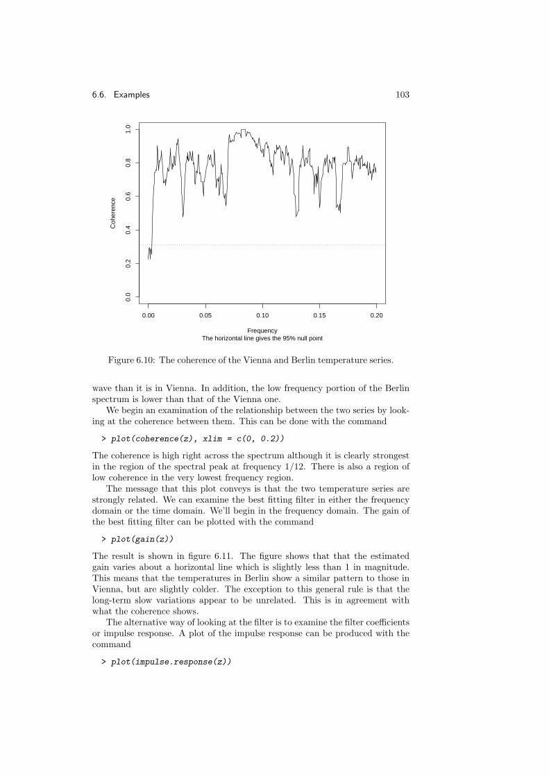
6.6. Examples 103
The horizontal line gives the 95% null pointFrequency
Coh
eren
ce
0.00 0.05 0.10 0.15 0.20
0.0
0.2
0.4
0.6
0.8
1.0
Figure 6.10: The coherence of the Vienna and Berlin temperature series.
wave than it is in Vienna. In addition, the low frequency portion of the Berlinspectrum is lower than that of the Vienna one.
We begin an examination of the relationship between the two series by look-ing at the coherence between them. This can be done with the command
> plot(coherence(z), xlim = c(0, 0.2))
The coherence is high right across the spectrum although it is clearly strongestin the region of the spectral peak at frequency 1/12. There is also a region oflow coherence in the very lowest frequency region.
The message that this plot conveys is that the two temperature series arestrongly related. We can examine the best fitting filter in either the frequencydomain or the time domain. We’ll begin in the frequency domain. The gain ofthe best fitting filter can be plotted with the command
> plot(gain(z))
The result is shown in figure 6.11. The figure shows that that the estimatedgain varies about a horizontal line which is slightly less than 1 in magnitude.This means that the temperatures in Berlin show a similar pattern to those inVienna, but are slightly colder. The exception to this general rule is that thelong-term slow variations appear to be unrelated. This is in agreement withwhat the coherence shows.
The alternative way of looking at the filter is to examine the filter coefficientsor impulse response. A plot of the impulse response can be produced with thecommand
> plot(impulse.response(z))

104 Chapter 6. Frequency Domain Analysis
Bandwidth = 0.00852, Degrees of freedom = 18Frequency
Gai
n
0.0 0.1 0.2 0.3 0.4 0.5
0.4
0.6
0.8
1.0
1.2
1.4
Figure 6.11: The gain of the filter which approximates the Berlin seriesusing the Vienna one.
−40 −20 0 20 40
0.0
0.2
0.4
0.6
0.8
Lag
Coe
ffice
nt
Figure 6.12: The coefficients of the filter which best approximates theBerlin series using the Vienna one.

6.6. Examples 105
This produces the result shown in figure 6.12. The plot shows that the averagemonthly temperatures in Berlin and Vienna move in step, with the temperaturein Berlin being between 0.8 and 0.9 times that in Vienna.
The cities of Berlin and Vienna are geographically close and weather systemspass between them in a matter of days. Because of this it should be no surprisethat the best fitting filter has the form that it does. What is surprising is thatthere is such a lack of similarity at the very lowest frequencies. This suggeststhat long term temperature variations are a local effect, possibly the result ofhuman activity.


![The Not Quite R (NQR) Project: Explorations Using the ...jay/JSM2011/KaneJSM2011.pdf · • Start from scratch, change the grammar (Duncan Temple-Lang and Ross Ihaka [3]) • R on](https://img.pdfslide.us/doc/110x75/5ec9dda1bb8ca67fb44657ff/the-not-quite-r-nqr-project-explorations-using-the-jayjsm2011-a-start.jpg)


![Introduction à [width=2cm,height=1.5cm]Rlogo · R´ef´erences R´ef´erences bibliographiques Ihaka R. and Gentleman R. (1996). R : a language for data analysis and graphics. Journal](https://img.pdfslide.us/doc/110x75/604f5ef9022e9c2c0252f2cd/introduction-width2cmheight15cmrlogo-references-references-bibliographiques.jpg)