Time Series Analysis

AutocorrelationNaive & Simple AveragingMoving AveragesExponential SmoothingRegression Analysis

Time Series Models

Trends: linear moving average, exponential smoothing,

Regression, growth curves Seasonality:

classical decomposition, multiple regression, time series & Box-Jenkins

Cyclical: classical decomposition, economic indicators,

econometric models, multiple regression and Box-Jenkins

Evaluating Methods

Forecasting method is selected - many times by intuition, previous experience, or computer resource availability

Divide the data into two sections - an initialization part and a test part

Use the forecast technique to determine the fitted values for the initialization data set

Use the forecast technique to forecast the test data set and determine the forecast errors

Evaluate errors (MAD, MPE, MSE, MAPE) Use the technique, modify, or develop new model

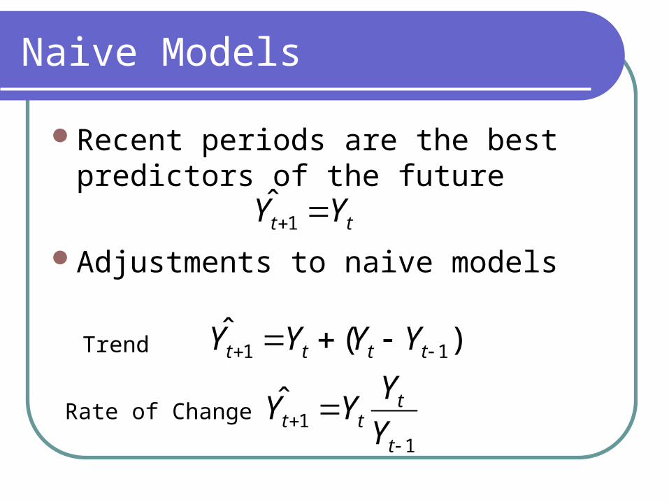
Naive Models

Recent periods are the best predictors of the future

Adjustments to naive models

tt YY 1ˆ

)(ˆ11 tttt YYYY

11

ˆ

t

ttt Y

YYY

Trend

Rate of Change

Period t Year Quarter Sales1 1990 1 5002 2 3503 3 2504 4 4005 1991 1 4506 2 3507 3 2008 4 3009 1992 1 35010 2 20011 3 15012 4 40013 1993 1 55014 2 35015 3 25016 4 55017 1994 1 55018 2 40019 3 35020 4 60021 1995 1 75022 2 50023 3 40024 4 65025 1996 1 85026 2 60027 3 45028 4 700

tt YY 1ˆ

65025 Y

Use 1990-95 as initializationUse 1996 as the test data set

Forecast the first period in 1996

Forecast error:

252525 YYe

65085025 e

Forecast for the remaining 1996 quarters and calculate the error - what do you see happening?

Naïve Models: Trended Data

Nonstationary - data values increase over time

)(ˆ11 tttt YYYY

900ˆ

)400650(650ˆ

)(ˆ

25

25

23242425

Y

Y

YYYY252525 YYe

90085025 e

Naïve Methods: Rate of Change

11

ˆ

t

ttt Y

YYY

400

650 650ˆ

ˆ

25

23

242425

Y

Y

YYY 252525 YYe

105685025 e

Can also use Naïve models for seasonal forecasts - data indicates that Quarter 1 seems to be higher than 2,3,4.

Averaging Methods

Simple Averages - quick, inexpensive (should only be used on stationary data)

Moving Averages - a constant number specified at the outset and a mean computed for the most recent observations - such as a 3 or 4 period moving average. Works best with stationary data. The larger the order of the moving average, the

greater the smoothing effect. Larger n when there are wide, infrequent fluctuations in the data.

By smoothing recent actual values, removes randomness.

Period t Year Quarter Sales1 1990 1 5002 2 3503 3 2504 4 4005 1991 1 4506 2 3507 3 2008 4 3009 1992 1 35010 2 20011 3 15012 4 40013 1993 1 55014 2 35015 3 25016 4 55017 1994 1 55018 2 40019 3 35020 4 60021 1995 1 75022 2 50023 3 40024 4 65025 1996 1 85026 2 60027 3 45028 4 700

If you suspect seasonality, with quarterly data, it makes sense to use a 4-period moving average (monthly data would use a 12 period moving average). The larger the number of periods, the smoother the fluctuations become.

575ˆ4

750500400650ˆ

4ˆ

25

25

2122232425

Y

Y

yyyyY

650ˆ4

850600450700ˆ

4ˆ

29

29

2526272829

Y

Y

yyyyY

275

575850

ˆ

25

25

252525

e

e

yye

Period t Year Quarter SalesMoving Total

MA Forecast et

1 1990 1 500 -2 2 350 -3 3 250 -4 4 400 1500 366.67 33.335 1991 1 450 1450 375.00 75.006 2 350 1450 362.50 -12.507 3 200 1400 362.50 -162.508 4 300 1300 350.00 -50.009 1992 1 350 1200 325.00 25.0010 2 200 1050 300.00 -100.0011 3 150 1000 262.50 -112.5012 4 400 1100 250.00 150.0013 1993 1 550 1300 275.00 275.0014 2 350 1450 325.00 25.0015 3 250 1550 362.50 -112.5016 4 550 1700 387.50 162.5017 1994 1 550 1700 425.00 125.0018 2 400 1750 425.00 -25.0019 3 350 1850 437.50 -87.5020 4 600 1900 462.50 137.5021 1995 1 750 2100 475.00 275.0022 2 500 2200 525.00 -25.0023 3 400 2250 550.00 -150.0024 4 650 2300 562.50 87.5025 1996 1 850 2400 575.00 275.0026 2 600 2500 600.00 0.0027 3 450 2550 625.00 -175.0028 4 700 2600 637.50 62.5029 1997 1 650.00

How many periods?

To determine how many periods to use for a moving average, remember: The smaller the number, the more weight given

to recent periods. A smaller number is desirable when there are

sudden shifts in the level of the series. The greater the number, less weight is given to

more recent periods. A larger number is desirable when there are

wide or infrequent fluctuations in the data

Double Moving Averages

Double Moving Averages - designed to handle trending data. One set of moving averages is calculated and then a second set is calculated as a moving average of the first set.

Weighted Moving Average - place more weight on recent observations. Sum of the weights needs to equal 1.

More on Moving Averages

Moving averages are used with quarterly or monthly data to help examine the components within a time series.

Used as a forecast, large-order moving averages pays very little attention to fluctuations in the data series

Minitab does a great job with SMA. However, you will need to use Excel to calculate DMA.

Moving average

Data RentsLength 15.0000NMissing 0

Moving Average Length: 3 Accuracy MeasuresMAPE: 1.404 MAD: 9.806 MSD: 132.676

Row Period Rents AVER1 Predict Error

1 1 654 * * * 2 2 658 * * * 3 3 665 659.000 * * 4 4 672 665.000 659.000 13.0000 5 5 673 670.000 665.000 8.0000 6 6 671 672.000 670.000 1.0000 7 7 693 679.000 672.000 21.0000 8 8 694 686.000 679.000 15.0000 9 9 701 696.000 686.000 15.0000 10 10 703 699.333 696.000 7.0000 11 11 702 702.000 699.333 2.6667 12 12 710 705.000 702.000 8.0000 13 13 712 708.000 705.000 7.0000 14 14 711 711.000 708.000 3.0000 15 15 728 717.000 711.000 17.0000

Row Period FORE1 Lower Upper

1 16 717 694.424 739.576

Stat, Time Series, Moving AverageEnter the variable name andthe number of periods - this example uses a 3 period moving average.MAPE, MAD and MSE (noted as MSD for Mean Squared Deviations) is automatically calculated.

Formulas for DMA

1. In Excel, Calculate a SMA.

2. Calculate the DMA from the SMA with a SMA using the same number of periods

3. Compute the differences between SMA and DMA. This value is noted as a.

4. Calculate an adjustment factor (similar to the slope in regression) that measures the change over the series, noted as b.

5. Calculate the forecast p periods into the future (usually 1)

6. Calculate the error for each period

ttt DMASMAa *2

average moving the in periods of number the is n where

ttt DMASMAn

b )(1

2

pbaY ttpt ˆ

Time Rents SMA DMA a b Forecast Error1 6542 6583 665 6594 672 6655 673 670 665 675 56 671 672 669 675 3 681 -107 693 679 674 684 5 678 158 694 686 679 693 7 690 49 701 696 687 705 9 700 1

10 703 699 694 705 6 714 -1111 702 702 699 705 3 710 -812 710 705 702 708 3 708 213 712 708 705 711 3 711 114 711 711 708 714 3 714 -315 728 717 712 722 5 717 1116 727

Weekly Rents DMA example

Cell Formulas

Excel has a built-in Moving Average function within the Data Analysis tool pack - but it is only a SMA.

Prediction Intervals

A good way to test to see if your model has good predictability to is look at the probability that the actual values will be within a 95% interval.

If n<30, use t/2,n-1

yxSzyActual 2/ˆ

Exponential Smoothing Methods

Single Exponential Smoothing (Averaging)

TrackingDouble Exponential SmoothingHolt’s MethodWinter’s Model

Exponential Smoothing Methods

Continually revising a forecast in light of more recent experiences. Averaging (smoothing) past values of a series in a decreasing (exponential) manner. The observations are weighted with more weight being given to the more recent observations

1- to valuesmoothed oldˆ

period in nobservationew

1)(0constant smoothing

periodnext for valuesmoothed ˆ

)ˆ(ˆˆ

1

1

tY

tY

newY

YYYY

t

t

t

tttt

Exponential Smoothing Methods When looking at the formula - it is really the old forecast plus

times the error in the old forecast To get started, we need a smoothing constant, an initial forecast,

and an actual value. Can use the first actual as the forecast value or you can average the first n observations. Minitab’s default is 6.

The smoothing constant serves as the weighting factor. When is close to 1, the new forecast will include a substantial adjustment for any error that occurred in the preceding forecast. When is close to 0, the new forecast is very similar to the old forecast. Iterative procedure to chose by minimizing MSE.

The smoothing constant is not an arbitrary choice - but generally falls between .1 and .5. If we want predictions to be stable and random variation smoothed, use a small . If we want a rapid response a larger value is required.

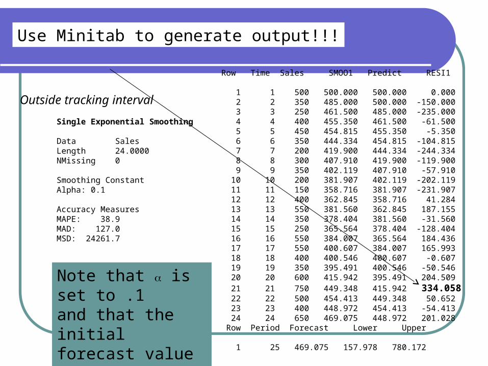
Use Minitab to generate output!!!

Single Exponential Smoothing

Data SalesLength 24.0000NMissing 0

Smoothing ConstantAlpha: 0.1 Accuracy Measures MAPE: 38.9 MAD: 127.0 MSD: 24261.7

Row Time Sales SMOO1 Predict RESI1

1 1 500 500.000 500.000 0.000 2 2 350 485.000 500.000 -150.000 3 3 250 461.500 485.000 -235.000 4 4 400 455.350 461.500 -61.500 5 5 450 454.815 455.350 -5.350 6 6 350 444.334 454.815 -104.815 7 7 200 419.900 444.334 -244.334 8 8 300 407.910 419.900 -119.900 9 9 350 402.119 407.910 -57.910 10 10 200 381.907 402.119 -202.119 11 11 150 358.716 381.907 -231.907 12 12 400 362.845 358.716 41.284 13 13 550 381.560 362.845 187.155 14 14 350 378.404 381.560 -31.560 15 15 250 365.564 378.404 -128.404 16 16 550 384.007 365.564 184.436 17 17 550 400.607 384.007 165.993 18 18 400 400.546 400.607 -0.607 19 19 350 395.491 400.546 -50.546 20 20 600 415.942 395.491 204.509 21 21 750 449.348 415.942 334.058 22 22 500 454.413 449.348 50.652 23 23 400 448.972 454.413 -54.413 24 24 650 469.075 448.972 201.028 Row Period Forecast Lower Upper

1 25 469.075 157.978 780.172

Note that is set to .1and that the initial forecast value is the first actual value

Outside tracking interval

Actual

Smoothed

Forecast

Actual

Smoothed

Forecast

0 10 20 30

150

250

350

450

550

650

750

850

Sal

es

Time

Smoothing Constant

Alpha:

MAPE:

MAD:

MSD:

0.100

37.0

134.9

27735.5

Sales data Single Exponential Smoothing .1

The small here smooths the data.

Row Time Sales Smooth Predict Error

1 1 500 500.000 500.000 0.000 2 2 350 410.000 500.000 -150.000 3 3 250 314.000 410.000 -160.000 4 4 400 365.600 314.000 86.000 5 5 450 416.240 365.600 84.400 6 6 350 376.496 416.240 -66.240 7 7 200 270.598 376.496 -176.496 8 8 300 288.239 270.598 29.402 9 9 350 325.296 288.239 61.761 10 10 200 250.118 325.296 -125.296 11 11 150 190.047 250.118 -100.118 12 12 400 316.019 190.047 209.953 13 13 550 456.408 316.019 233.981 14 14 350 392.563 456.408 -106.408 15 15 250 307.025 392.563 -142.563 16 16 550 452.810 307.025 242.975 17 17 550 511.124 452.810 97.190 18 18 400 444.450 511.124 -111.124 19 19 350 387.780 444.450 -94.450 20 20 600 515.112 387.780 212.220 21 21 750 656.045 515.112 234.888 22 22 500 562.418 656.045 -156.045 23 23 400 464.967 562.418 -162.418 24 24 650 575.987 464.967 185.033

Row Period Forecast Lower Upper

1 25 575.987 246.364 905.610

Single Exponential Smoothing

Data SalesLength 24.0000NMissing 0

Smoothing ConstantAlpha: 0.6 Accuracy Measures MAPE: 36.5 MAD: 134.5 MSD: 22248.4

You can only forecast for 1 period - because the formula requires actual data from the current period. If you forecast more than 1 period, it will remain the same as a 1 period forecast.

Actual

Smoothed

Forecast

Actual

Smoothed

Forecast

0 5 10 15 20 25

140

240

340

440

540

640

740

840

940

Sal

es

Time

Smoothing Constant

Alpha:

MAPE:

MAD:

MSD:

0.600

36.5

134.5

22248.4

Sales data Single Exponential Smoothing .6

The large in this example responds quickly to the data.

Tracking

Use a tracking signal (measure of errors over time) and setting limits. For example, if we forecast 10 periods, count the number of negative and positive errors. If the number of positive errors is substantially less or greater than n/2, then the process is out of control.

Can also use 95% prediction interval (1.96 * sqrt (MSE)). If the forecast error is outside of the interval, use a new optimal .

Looking back at the .1 single exponential smoothing:1.96*sqrt(24261) = +-305 Observation #21 is out-of-control. We

need to re-evaluate alpha level because this technique is biased.

Double Exponential Smoothing

Also known as Brown’s Method. Used to forecast a series with a linear trend.

tat time Y valuesmoothedlly exponentiadoubly A

tat time Y valuesmoothedlly exponentia

t't

t

tA

)(1

2

)1(

)1(

'

'

'1

'

1

ttt

ttt

ttt

ttt

AAb

AAa

AAA

AYA

future theinto periods is p where

pbaY ttpt

Double Exponential Smoothing

Uses a single coefficient, alpha, for both smoothing operations. Calculates the difference between single and double smoothed values as a measure of trend (at). It then adds this value to the single smoothed value together with an adjustment for the current trend (bt).

In Minitab, use the same value for the trend and level. Do NOT optimize for Brown’s Method!

Minitab sets the initial value for the smoothed series and trend adjustment by calculating the trend’s slope and intercept using the least square’s method.

If you use Excel, use the Actual values of period 1 to estimate the single and double exponentially smoothed values. Realize that Excel is assuming there is no trend present and will tend to underestimate!

Before running Brown’s method; here is single exponential for Rental data with set to .2

Actual

Smoothed

Forecast

Actual

Smoothed

Forecast

0 5 10 15

650

660

670

680

690

700

710

720

730

740

750

Re

nts

Time

Smoothing Constant

Alpha:

MAPE:

MAD:

MSD:

0.200

2.437

17.014

361.330

Rents data Single Exponential Smoothing .2

Row Time Rents Smooth Predict Error

1 1 654 654.750 655.250 -1.2500 2 2 658 658.891 659.486 -1.4857 3 3 665 664.034 663.389 1.6106 4 4 672 670.074 668.789 3.2107 5 5 673 674.406 675.343 -2.3430 6 6 671 675.980 679.300 -8.3003 7 7 693 684.928 679.547 13.4533 8 8 694 691.988 690.647 3.3530 9 9 701 699.346 698.244 2.7563 10 10 703 704.826 706.043 -3.0427 11 11 702 707.421 711.035 -9.0353 12 12 710 711.311 712.185 -2.1852 13 13 712 714.235 715.725 -3.7255 14 14 711 715.232 718.054 -7.0536 15 15 728 721.953 717.922 10.0781

Row Period Forecast Lower Upper

1 16 726.255 714.351 738.160

Double Exponential Smoothing

Data RentsLength 15.0000NMissing 0

Smoothing ConstantsAlpha (level): 0.4 Gamma (trend): 0.4 Accuracy Measures MAPE: 0.6978 MAD: 4.8589 MSD: 36.7840

The SMOOTH value is a Minitab does NOT output the value of b you can calculate the value of b1 by taking Prediction for period 2 and subtracting the Smooth value for period 1. You can store the b in Mintab by selecting the TREND option in Results.

Actual

Smoothed

Forecast

Actual

Smoothed

Forecast

0 5 10 15

650

660

670

680

690

700

710

720

730

740

Re

nts

Time

Smoothing Constants

Alpha (level):

Gamma (trend):

MAPE:

MAD:

MSD:

0.400

0.400

0.6978

4.8589

36.7840

Rentals Double Exponential Smoothing .4

Notice that the MSE is much lower than single exponential smoothing and that the smoothed value is much closer to the data. This is due to the trending.

Actual

Smoothed

Forecast

Actual

Smoothed

Forecast

0 5 10 15

650

700

750

Re

nts

Time

Smoothing Constants

Alpha (level):

Gamma (trend):

MAPE:

MAD:

MSD:

0.900

0.900

0.9006

6.2924

81.1959

Rentals Double Exponential Smoothing .9

Remember, large responds rapidly to the data.

Actual

Smoothed

Forecast

Actual

Smoothed

Forecast

0 5 10 15

650

660

670

680

690

700

710

720

730

740

Re

nts

Time

Smoothing Constants

Alpha (level):

Gamma (trend):

MAPE:

MAD:

MSD:

0.100

0.100

0.5729

3.9757

24.4308

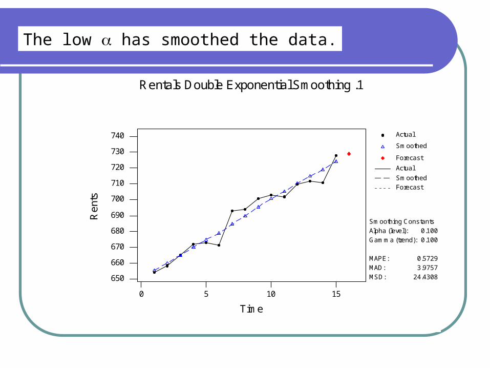
Rentals Double Exponential Smoothing .1

The low has smoothed the data.

Setting the best

The level should always be between 0 and 1. However, Minitab is known for violating this rule. We will generally use .1 to .5. It becomes an art and a science in picking the “correct” level - stay with the objective of minimizing MSE. This may require running different levels and comparing MSE values.

Holt’s Method

Extension of Brown’s double exponential smoothing but it uses two coefficients.

is the smoothing constant for the level is the trend smoothing constant - used

to remove random errorUsing Minitab, select the OPTIMAL - but

realize, Minitab will violate the between 0 and 1.

Winter’s Method

Extends Holt’s Method to include an estimate for seasonality.

is the smoothing constant for the level is the trend smoothing constant - used to remove

random error smoothing constant for seasonality This fun formula removes seasonal effects. The

forecast is modified by multiplying by a seasonal index. We will calculate this seasonal index in Chapter 8.

Row Time Sales Smooth Predict Error

1 1 500 615.051 563.257 -63.257 2 2 350 365.798 328.859 21.141 3 3 250 249.233 222.565 27.435 4 4 400 421.495 375.344 24.656 5 5 450 415.817 367.063 82.937 6 6 350 281.175 249.255 100.745 7 7 200 216.030 195.221 4.779 8 8 300 352.436 315.576 -15.576 9 9 350 342.438 300.945 49.055 10 10 200 230.704 202.255 -2.255 11 11 150 141.989 121.863 28.137 12 12 400 234.808 201.294 198.706 13 13 550 322.295 292.949 257.051 14 14 350 276.632 263.306 86.694 15 15 250 218.565 211.335 38.665 16 16 550 434.487 423.599 126.401 17 17 550 539.216 532.584 17.416 18 18 400 355.337 351.428 48.572 19 19 350 266.412 264.999 85.001 20 20 600 582.413 586.284 13.716 21 21 750 645.882 650.706 99.294 22 22 500 462.731 468.626 31.374 23 23 400 354.980 360.255 39.745 24 24 650 699.938 712.712 -62.712 Row Period Forecast Lower Upper 1 25 778.179 622.470 933.889 2 26 521.917 352.933 690.902 3 27 393.430 209.778 577.082 4 28 716.726 517.321 916.132

Winters' multiplicative model

Data SalesLength 24.0000NMissing 0

Smoothing Constants Alpha (level): 0.4Gamma (trend): 0.1Delta (seasonal): 0.3 Accuracy Measures MAPE: 15.21 MAD: 63.55 MSD: 7636.86

Multiplicative model because we are multiplying the seasonal index by the current smoothed and trend values. Can use the Storage option to store trend and seasonal results.

Actual

Smoothed

Forecast

Actual

Smoothed

Forecast

0 5 10 15 20 25

100

200

300

400

500

600

700

800

900

Sal

es

Time

Smoothing ConstantsAlpha (level):

Gamma (trend):Delta (season):

MAPE:MAD:

MSD:

0.400

0.1000.300

15.21 63.55

7636.86

Winter's Method Sales Data

More on Winter’s

In order to Forecast, you would need to have all three estimates. Use Minitab to forecast.

On the exam, you would be required to state the forecast from the output. For Brown’s, Holt, & Winter’s you will not need to calculate a forecast. You should be able to calculate a forecast for Moving averages and Simple exponential smoothing. You should also be able to develop Prediction intervals, track the forecast, and determine the best forecast by comparing MSEs.

Do not try to memorize formula’s but do know the differences between Models

For next time

We will run all models from Chapter 4 and compare with MSE and also track the errors based on 95% intervals using the data from Case 3.3. Key in this data.