Embed Size (px)
Citation preview


For other titles published in this series, go to
G. Casella S. Fienberg I. Olkin
www.springer.com/series/417
Series Editors
Springer Texts in Statistics

Robert H. Shumway • David S. Stoffer
With R Examples
Its Applications
Third edition
Time Series Analysis and

subject to proprietary rights. Printed on acid-free paper Springer is part of Springer Science+Business Media (www.springer.com)
ISSN 1431-875X
Springer New York Dordrecht Heidelberg London
© Springer Science+Business Media, LLC 2011All rights reserved. This work may not be translated or copied in whole or in part without the writtenpermission of the publisher (Springer Science+Business Media, LLC, 233 Spring Street, New York,NY 10013, USA), except for brief excerpts in connection with reviews or scholarly analysis. Use in connection with any form of information storage and retrieval, electronic adaptation, computer software, or by similar or dissimilar methodology now known or hereafter developed is forbidden. The use in this publication of trade names, trademarks, service marks, and similar terms, even if they are not identified as such, is not to be taken as an expression of opinion as to whether or not they are
ISBN 978-1-4419-7864-6 DOI 10.1007/978-1-4419-7865-3
University of CaliforniaDavis, California
Department of Statistics
USA
Department of Statistics University of Pittsburgh Pittsburgh, Pennsylvania
Prof. David S. Stoffer
e-ISBN 978-1-4419-7865-3
USA
Prof. Robert H. Shumway

To my wife, Ruth, for her support and joie de vivre, and to thememory of my thesis adviser, Solomon Kullback.
R.H.S.
To my family and friends, who constantly remind me what isimportant.
D.S.S.

Preface to the Third Edition
The goals of this book are to develop an appreciation for the richness andversatility of modern time series analysis as a tool for analyzing data, and stillmaintain a commitment to theoretical integrity, as exemplified by the seminalworks of Brillinger (1975) and Hannan (1970) and the texts by Brockwell andDavis (1991) and Fuller (1995). The advent of inexpensive powerful computinghas provided both real data and new software that can take one considerablybeyond the fitting of simple time domain models, such as have been elegantlydescribed in the landmark work of Box and Jenkins (1970). This book isdesigned to be useful as a text for courses in time series on several differentlevels and as a reference work for practitioners facing the analysis of time-correlated data in the physical, biological, and social sciences.
We have used earlier versions of the text at both the undergraduate andgraduate levels over the past decade. Our experience is that an undergraduatecourse can be accessible to students with a background in regression analysisand may include §1.1–§1.6, §2.1–§2.3, the results and numerical parts of §3.1–§3.9, and briefly the results and numerical parts of §4.1–§4.6. At the advancedundergraduate or master’s level, where the students have some mathematicalstatistics background, more detailed coverage of the same sections, with theinclusion of §2.4 and extra topics from Chapter 5 or Chapter 6 can be used asa one-semester course. Often, the extra topics are chosen by the students ac-cording to their interests. Finally, a two-semester upper-level graduate coursefor mathematics, statistics, and engineering graduate students can be craftedby adding selected theoretical appendices. For the upper-level graduate course,we should mention that we are striving for a broader but less rigorous levelof coverage than that which is attained by Brockwell and Davis (1991), theclassic entry at this level.
The major difference between this third edition of the text and the secondedition is that we provide R code for almost all of the numerical examples. Inaddition, we provide an R supplement for the text that contains the data andscripts in a compressed file called tsa3.rda; the supplement is available on thewebsite for the third edition, http://www.stat.pitt.edu/stoffer/tsa3/,

viii Preface to the Third Edition
or one of its mirrors. On the website, we also provide the code used in eachexample so that the reader may simply copy-and-paste code directly into R.Specific details are given in Appendix R and on the website for the text.Appendix R is new to this edition, and it includes a small R tutorial as wellas providing a reference for the data sets and scripts included in tsa3.rda. Sothere is no misunderstanding, we emphasize the fact that this text is abouttime series analysis, not about R. R code is provided simply to enhance theexposition by making the numerical examples reproducible.
We have tried, where possible, to keep the problem sets in order so that aninstructor may have an easy time moving from the second edition to the thirdedition. However, some of the old problems have been revised and there aresome new problems. Also, some of the data sets have been updated. We addedone section in Chapter 5 on unit roots and enhanced some of the presenta-tions throughout the text. The exposition on state-space modeling, ARMAXmodels, and (multivariate) regression with autocorrelated errors in Chapter 6have been expanded. In this edition, we use standard R functions as much aspossible, but we use our own scripts (included in tsa3.rda) when we feel itis necessary to avoid problems with a particular R function; these problemsare discussed in detail on the website for the text under R Issues.
We thank John Kimmel, Executive Editor, Springer Statistics, for his guid-ance in the preparation and production of this edition of the text. We aregrateful to Don Percival, University of Washington, for numerous suggestionsthat led to substantial improvement to the presentation in the second edition,and consequently in this edition. We thank Doug Wiens, University of Alberta,for help with some of the R code in Chapters 4 and 7, and for his many sug-gestions for improvement of the exposition. We are grateful for the continuedhelp and advice of Pierre Duchesne, University of Montreal, and AlexanderAue, University of California, Davis. We also thank the many students andother readers who took the time to mention typographical errors and othercorrections to the first and second editions. Finally, work on the this editionwas supported by the National Science Foundation while one of us (D.S.S.)was working at the Foundation under the Intergovernmental Personnel Act.
Davis, CA Robert H. ShumwayPittsburgh, PA David S. StofferSeptember 2010
Contents
Preface to the Third Edition . . . . . . . . . . . . . . . . . . . . . . . . . . . . . . . . . . . vii
1 Characteristics of Time Series . . . . . . . . . . . . . . . . . . . . . . . . . . . . . 11.1 Introduction . . . . . . . . . . . . . . . . . . . . . . . . . . . . . . . . . . . . . . . . . . . . 11.2 The Nature of Time Series Data . . . . . . . . . . . . . . . . . . . . . . . . . . . 31.3 Time Series Statistical Models . . . . . . . . . . . . . . . . . . . . . . . . . . . . 111.4 Measures of Dependence: Autocorrelation and
Cross-Correlation . . . . . . . . . . . . . . . . . . . . . . . . . . . . . . . . . . . . . . . . 171.5 Stationary Time Series . . . . . . . . . . . . . . . . . . . . . . . . . . . . . . . . . . . 221.6 Estimation of Correlation . . . . . . . . . . . . . . . . . . . . . . . . . . . . . . . . . 281.7 Vector-Valued and Multidimensional Series . . . . . . . . . . . . . . . . . 33Problems . . . . . . . . . . . . . . . . . . . . . . . . . . . . . . . . . . . . . . . . . . . . . . . . . . . 39
2 Time Series Regression and Exploratory Data Analysis . . . . 472.1 Introduction . . . . . . . . . . . . . . . . . . . . . . . . . . . . . . . . . . . . . . . . . . . . 472.2 Classical Regression in the Time Series Context . . . . . . . . . . . . . 482.3 Exploratory Data Analysis . . . . . . . . . . . . . . . . . . . . . . . . . . . . . . . . 572.4 Smoothing in the Time Series Context . . . . . . . . . . . . . . . . . . . . . 70Problems . . . . . . . . . . . . . . . . . . . . . . . . . . . . . . . . . . . . . . . . . . . . . . . . . . . 78
3 ARIMA Models . . . . . . . . . . . . . . . . . . . . . . . . . . . . . . . . . . . . . . . . . . . 833.1 Introduction . . . . . . . . . . . . . . . . . . . . . . . . . . . . . . . . . . . . . . . . . . . 833.2 Autoregressive Moving Average Models . . . . . . . . . . . . . . . . . . . . 843.3 Difference Equations . . . . . . . . . . . . . . . . . . . . . . . . . . . . . . . . . . . . . 973.4 Autocorrelation and Partial Autocorrelation . . . . . . . . . . . . . . . . 1023.5 Forecasting . . . . . . . . . . . . . . . . . . . . . . . . . . . . . . . . . . . . . . . . . . . . 1083.6 Estimation . . . . . . . . . . . . . . . . . . . . . . . . . . . . . . . . . . . . . . . . . . . . . 1213.7 Integrated Models for Nonstationary Data . . . . . . . . . . . . . . . . . 1413.8 Building ARIMA Models . . . . . . . . . . . . . . . . . . . . . . . . . . . . . . . . 1443.9 Multiplicative Seasonal ARIMA Models . . . . . . . . . . . . . . . . . . . . 154Problems . . . . . . . . . . . . . . . . . . . . . . . . . . . . . . . . . . . . . . . . . . . . . . . . . . . 162
x Contents
4 Spectral Analysis and Filtering . . . . . . . . . . . . . . . . . . . . . . . . . . . . 1734.1 Introduction . . . . . . . . . . . . . . . . . . . . . . . . . . . . . . . . . . . . . . . . . . . . 1734.2 Cyclical Behavior and Periodicity . . . . . . . . . . . . . . . . . . . . . . . . . . 1754.3 The Spectral Density . . . . . . . . . . . . . . . . . . . . . . . . . . . . . . . . . . . . 1804.4 Periodogram and Discrete Fourier Transform . . . . . . . . . . . . . . . 1874.5 Nonparametric Spectral Estimation . . . . . . . . . . . . . . . . . . . . . . . . 1964.6 Parametric Spectral Estimation . . . . . . . . . . . . . . . . . . . . . . . . . . . 2124.7 Multiple Series and Cross-Spectra . . . . . . . . . . . . . . . . . . . . . . . . . 2164.8 Linear Filters . . . . . . . . . . . . . . . . . . . . . . . . . . . . . . . . . . . . . . . . . . . 2214.9 Dynamic Fourier Analysis and Wavelets . . . . . . . . . . . . . . . . . . . . 2284.10 Lagged Regression Models . . . . . . . . . . . . . . . . . . . . . . . . . . . . . . . . 2424.11 Signal Extraction and Optimum Filtering . . . . . . . . . . . . . . . . . . . 2474.12 Spectral Analysis of Multidimensional Series . . . . . . . . . . . . . . . . 252Problems . . . . . . . . . . . . . . . . . . . . . . . . . . . . . . . . . . . . . . . . . . . . . . . . . . . 255
5 Additional Time Domain Topics . . . . . . . . . . . . . . . . . . . . . . . . . . . 2675.1 Introduction . . . . . . . . . . . . . . . . . . . . . . . . . . . . . . . . . . . . . . . . . . . . 2675.2 Long Memory ARMA and Fractional Differencing . . . . . . . . . . . 2675.3 Unit Root Testing . . . . . . . . . . . . . . . . . . . . . . . . . . . . . . . . . . . . . . . 2775.4 GARCH Models . . . . . . . . . . . . . . . . . . . . . . . . . . . . . . . . . . . . . . . . 2805.5 Threshold Models . . . . . . . . . . . . . . . . . . . . . . . . . . . . . . . . . . . . . . . 2895.6 Regression with Autocorrelated Errors . . . . . . . . . . . . . . . . . . . . . 2935.7 Lagged Regression: Transfer Function Modeling . . . . . . . . . . . . . 2965.8 Multivariate ARMAX Models . . . . . . . . . . . . . . . . . . . . . . . . . . . . . 301Problems . . . . . . . . . . . . . . . . . . . . . . . . . . . . . . . . . . . . . . . . . . . . . . . . . . . 315
6 State-Space Models . . . . . . . . . . . . . . . . . . . . . . . . . . . . . . . . . . . . . . . . 3196.1 Introduction . . . . . . . . . . . . . . . . . . . . . . . . . . . . . . . . . . . . . . . . . . . 3196.2 Filtering, Smoothing, and Forecasting . . . . . . . . . . . . . . . . . . . . . 3256.3 Maximum Likelihood Estimation . . . . . . . . . . . . . . . . . . . . . . . . . 3356.4 Missing Data Modifications . . . . . . . . . . . . . . . . . . . . . . . . . . . . . . 3446.5 Structural Models: Signal Extraction and Forecasting . . . . . . . . 3506.6 State-Space Models with Correlated Errors . . . . . . . . . . . . . . . . . 354
6.6.1 ARMAX Models . . . . . . . . . . . . . . . . . . . . . . . . . . . . . . . . . . 3556.6.2 Multivariate Regression with Autocorrelated Errors . . . . 356
6.7 Bootstrapping State-Space Models . . . . . . . . . . . . . . . . . . . . . . . . 3596.8 Dynamic Linear Models with Switching . . . . . . . . . . . . . . . . . . . . 3656.9 Stochastic Volatility . . . . . . . . . . . . . . . . . . . . . . . . . . . . . . . . . . . . . 3786.10 Nonlinear and Non-normal State-Space Models Using Monte
Carlo Methods . . . . . . . . . . . . . . . . . . . . . . . . . . . . . . . . . . . . . . . . . 387Problems . . . . . . . . . . . . . . . . . . . . . . . . . . . . . . . . . . . . . . . . . . . . . . . . . . . 398

Contents xi
7 Statistical Methods in the Frequency Domain . . . . . . . . . . . . . 4057.1 Introduction . . . . . . . . . . . . . . . . . . . . . . . . . . . . . . . . . . . . . . . . . . . . 4057.2 Spectral Matrices and Likelihood Functions . . . . . . . . . . . . . . . . . 4097.3 Regression for Jointly Stationary Series . . . . . . . . . . . . . . . . . . . . 4107.4 Regression with Deterministic Inputs . . . . . . . . . . . . . . . . . . . . . . 4207.5 Random Coefficient Regression . . . . . . . . . . . . . . . . . . . . . . . . . . . 4297.6 Analysis of Designed Experiments . . . . . . . . . . . . . . . . . . . . . . . . . 4347.7 Discrimination and Cluster Analysis . . . . . . . . . . . . . . . . . . . . . . . 4507.8 Principal Components and Factor Analysis . . . . . . . . . . . . . . . . . 4687.9 The Spectral Envelope . . . . . . . . . . . . . . . . . . . . . . . . . . . . . . . . . . 485Problems . . . . . . . . . . . . . . . . . . . . . . . . . . . . . . . . . . . . . . . . . . . . . . . . . . . 501
Appendix A: Large Sample Theory . . . . . . . . . . . . . . . . . . . . . . . . . . . . 507A.1 Convergence Modes . . . . . . . . . . . . . . . . . . . . . . . . . . . . . . . . . . . . . . 507A.2 Central Limit Theorems . . . . . . . . . . . . . . . . . . . . . . . . . . . . . . . . . . 515A.3 The Mean and Autocorrelation Functions . . . . . . . . . . . . . . . . . . . 518
Appendix B: Time Domain Theory . . . . . . . . . . . . . . . . . . . . . . . . . . . . 527B.1 Hilbert Spaces and the Projection Theorem . . . . . . . . . . . . . . . . . 527B.2 Causal Conditions for ARMA Models . . . . . . . . . . . . . . . . . . . . . . 531B.3 Large Sample Distribution of the AR(p) Conditional Least
Squares Estimators . . . . . . . . . . . . . . . . . . . . . . . . . . . . . . . . . . . . . . 533B.4 The Wold Decomposition . . . . . . . . . . . . . . . . . . . . . . . . . . . . . . . . . 537
Appendix C: Spectral Domain Theory . . . . . . . . . . . . . . . . . . . . . . . . . 539C.1 Spectral Representation Theorem . . . . . . . . . . . . . . . . . . . . . . . . . . 539C.2 Large Sample Distribution of the DFT and Smoothed
Periodogram . . . . . . . . . . . . . . . . . . . . . . . . . . . . . . . . . . . . . . . . . . . . 543C.3 The Complex Multivariate Normal Distribution . . . . . . . . . . . . . 554
Appendix R: R Supplement . . . . . . . . . . . . . . . . . . . . . . . . . . . . . . . . . . . 559R.1 First Things First . . . . . . . . . . . . . . . . . . . . . . . . . . . . . . . . . . . . . . . 559
R.1.1 Included Data Sets . . . . . . . . . . . . . . . . . . . . . . . . . . . . . . . . 560R.1.2 Included Scripts . . . . . . . . . . . . . . . . . . . . . . . . . . . . . . . . . . . 562
R.2 Getting Started . . . . . . . . . . . . . . . . . . . . . . . . . . . . . . . . . . . . . . . . . 567R.3 Time Series Primer . . . . . . . . . . . . . . . . . . . . . . . . . . . . . . . . . . . . . . 571
References . . . . . . . . . . . . . . . . . . . . . . . . . . . . . . . . . . . . . . . . . . . . . . . . . . . . . 577
Index . . . . . . . . . . . . . . . . . . . . . . . . . . . . . . . . . . . . . . . . . . . . . . . . . . . . . . . . . . 591


1
Characteristics of Time Series
1.1 Introduction
The analysis of experimental data that have been observed at different pointsin time leads to new and unique problems in statistical modeling and infer-ence. The obvious correlation introduced by the sampling of adjacent pointsin time can severely restrict the applicability of the many conventional statis-tical methods traditionally dependent on the assumption that these adjacentobservations are independent and identically distributed. The systematic ap-proach by which one goes about answering the mathematical and statisticalquestions posed by these time correlations is commonly referred to as timeseries analysis.
The impact of time series analysis on scientific applications can be par-tially documented by producing an abbreviated listing of the diverse fieldsin which important time series problems may arise. For example, many fa-miliar time series occur in the field of economics, where we are continuallyexposed to daily stock market quotations or monthly unemployment figures.
ments. An epidemiologist might be interested in the number of influenza casesobserved over some time period. In medicine, blood pressure measurementstraced over time could be useful for evaluating drugs used in treating hy-pertension. Functional magnetic resonance imaging of brain-wave time seriespatterns might be used to study how the brain reacts to certain stimuli undervarious experimental conditions.
Many of the most intensive and sophisticated applications of time seriesmethods have been to problems in the physical and environmental sciences.This fact accounts for the basic engineering flavor permeating the language oftime series analysis. One of the earliest recorded series is the monthly sunspotnumbers studied by Schuster (1906). More modern investigations may cen-ter on whether a warming is present in global temperature measurements
1
Social scientists follow population series, such as birthrates or school enroll-
Springer Texts in Statistics, DOI 10.1007/978-1-4419-7865-3_1, © Springer Science+Business Media, LLC 2011
R.H. Shumway and D.S. Stoffer, Time Series Analysis and Its Applications: With R Examples,
2 1 Characteristics of Time Series
or whether levels of pollution may influence daily mortality in Los Angeles.The modeling of speech series is an important problem related to the efficienttransmission of voice recordings. Common features in a time series character-istic known as the power spectrum are used to help computers recognize andtranslate speech. Geophysical time series such as those produced by yearly de-positions of various kinds can provide long-range proxies for temperature andrainfall. Seismic recordings can aid in mapping fault lines or in distinguishingbetween earthquakes and nuclear explosions.
The above series are only examples of experimental databases that canbe used to illustrate the process by which classical statistical methodologycan be applied in the correlated time series framework. In our view, the firststep in any time series investigation always involves careful scrutiny of therecorded data plotted over time. This scrutiny often suggests the method ofanalysis as well as statistics that will be of use in summarizing the informationin the data. Before looking more closely at the particular statistical methods,it is appropriate to mention that two separate, but not necessarily mutuallyexclusive, approaches to time series analysis exist, commonly identified as thetime domain approach and the frequency domain approach.
The time domain approach is generally motivated by the presumptionthat correlation between adjacent points in time is best explained in termsof a dependence of the current value on past values. The time domain ap-proach focuses on modeling some future value of a time series as a parametricfunction of the current and past values. In this scenario, we begin with linearregressions of the present value of a time series on its own past values andon the past values of other series. This modeling leads one to use the resultsof the time domain approach as a forecasting tool and is particularly popularwith economists for this reason.
One approach, advocated in the landmark work of Box and Jenkins (1970;see also Box et al., 1994), develops a systematic class of models called au-toregressive integrated moving average (ARIMA) models to handle time-correlated modeling and forecasting. The approach includes a provision fortreating more than one input series through multivariate ARIMA or throughtransfer function modeling. The defining feature of these models is that theyare multiplicative models, meaning that the observed data are assumed toresult from products of factors involving differential or difference equationoperators responding to a white noise input.
A more recent approach to the same problem uses additive models morefamiliar to statisticians. In this approach, the observed data are assumed toresult from sums of series, each with a specified time series structure; for exam-ple, in economics, assume a series is generated as the sum of trend, a seasonaleffect, and error. The state-space model that results is then treated by makingjudicious use of the celebrated Kalman filters and smoothers, developed origi-nally for estimation and control in space applications. Two relatively completepresentations from this point of view are in Harvey (1991) and Kitagawa andGersch (1996). Time series regression is introduced in Chapter 2, and ARIMA

1.2 The Nature of Time Series Data 3
and related time domain models are studied in Chapter 3, with the empha-sis on classical, statistical, univariate linear regression. Special topics on timedomain analysis are covered in Chapter 5; these topics include modern treat-ments of, for example, time series with long memory and GARCH modelsfor the analysis of volatility. The state-space model, Kalman filtering andsmoothing, and related topics are developed in Chapter 6.
Conversely, the frequency domain approach assumes the primary charac-teristics of interest in time series analyses relate to periodic or systematicsinusoidal variations found naturally in most data. These periodic variationsare often caused by biological, physical, or environmental phenomena of inter-est. A series of periodic shocks may influence certain areas of the brain; windmay affect vibrations on an airplane wing; sea surface temperatures causedby El Nino oscillations may affect the number of fish in the ocean. The studyof periodicity extends to economics and social sciences, where one may beinterested in yearly periodicities in such series as monthly unemployment ormonthly birth rates.
In spectral analysis, the partition of the various kinds of periodic variationin a time series is accomplished by evaluating separately the variance associ-ated with each periodicity of interest. This variance profile over frequency iscalled the power spectrum. In our view, no schism divides time domain andfrequency domain methodology, although cliques are often formed that advo-cate primarily one or the other of the approaches to analyzing data. In manycases, the two approaches may produce similar answers for long series, butthe comparative performance over short samples is better done in the timedomain. In some cases, the frequency domain formulation simply provides aconvenient means for carrying out what is conceptually a time domain calcu-lation. Hopefully, this book will demonstrate that the best path to analyzingmany data sets is to use the two approaches in a complementary fashion. Ex-positions emphasizing primarily the frequency domain approach can be foundin Bloomfield (1976, 2000), Priestley (1981), or Jenkins and Watts (1968).On a more advanced level, Hannan (1970), Brillinger (1981, 2001), Brockwelland Davis (1991), and Fuller (1996) are available as theoretical sources. Ourcoverage of the frequency domain is given in Chapters 4 and 7.
The objective of this book is to provide a unified and reasonably completeexposition of statistical methods used in time series analysis, giving seriousconsideration to both the time and frequency domain approaches. Because amyriad of possible methods for analyzing any particular experimental seriescan exist, we have integrated real data from a number of subject fields intothe exposition and have suggested methods for analyzing these data.
1.2 The Nature of Time Series Data
Some of the problems and questions of interest to the prospective time se-ries analyst can best be exposed by considering real experimental data taken

4 1 Characteristics of Time Series
Fig. 1.1. Johnson & Johnson quarterly earnings per share, 84 quarters, 1960-I to1980-IV.
from different subject areas. The following cases illustrate some of the com-mon kinds of experimental time series data as well as some of the statisticalquestions that might be asked about such data.
Example 1.1 Johnson & Johnson Quarterly Earnings
Figure 1.1 shows quarterly earnings per share for the U.S. company Johnson& Johnson, furnished by Professor Paul Griffin (personal communication) ofthe Graduate School of Management, University of California, Davis. Thereare 84 quarters (21 years) measured from the first quarter of 1960 to thelast quarter of 1980. Modeling such series begins by observing the primarypatterns in the time history. In this case, note the gradually increasing un-derlying trend and the rather regular variation superimposed on the trendthat seems to repeat over quarters. Methods for analyzing data such as theseare explored in Chapter 2 (see Problem 2.1) using regression techniques andin Chapter 6, §6.5, using structural equation modeling.
To plot the data using the R statistical package, type the following:1
1 load("tsa3.rda") # SEE THE FOOTNOTE
2 plot(jj, type="o", ylab="Quarterly Earnings per Share")
Example 1.2 Global Warming
Consider the global temperature series record shown in Figure 1.2. The dataare the global mean land–ocean temperature index from 1880 to 2009, with
1 We assume that tsa3.rda has been downloaded to a convenient directory. SeeAppendix R for further details.

1.2 The Nature of Time Series Data 5
Fig. 1.2. Yearly average global temperature deviations (1880–2009) in degrees centi-grade.
the base period 1951-1980. In particular, the data are deviations, measuredin degrees centigrade, from the 1951-1980 average, and are an update ofHansen et al. (2006). We note an apparent upward trend in the series duringthe latter part of the twentieth century that has been used as an argumentfor the global warming hypothesis. Note also the leveling off at about 1935and then another rather sharp upward trend at about 1970. The question ofinterest for global warming proponents and opponents is whether the overalltrend is natural or whether it is caused by some human-induced interface.Problem 2.8 examines 634 years of glacial sediment data that might be takenas a long-term temperature proxy. Such percentage changes in temperaturedo not seem to be unusual over a time period of 100 years. Again, thequestion of trend is of more interest than particular periodicities.
The R code for this example is similar to the code in Example 1.1:1 plot(gtemp, type="o", ylab="Global Temperature Deviations")
Example 1.3 Speech Data
More involved questions develop in applications to the physical sciences.Figure 1.3 shows a small .1 second (1000 point) sample of recorded speechfor the phrase aaa · · ·hhh, and we note the repetitive nature of the signaland the rather regular periodicities. One current problem of great inter-est is computer recognition of speech, which would require converting thisparticular signal into the recorded phrase aaa · · ·hhh. Spectral analysis canbe used in this context to produce a signature of this phrase that can becompared with signatures of various library syllables to look for a match.
6 1 Characteristics of Time Series
Time
spee
ch
0 200 400 600 800 1000
010
0020
0030
0040
00
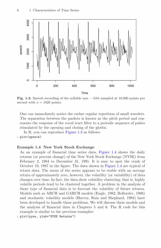
Fig. 1.3. Speech recording of the syllable aaa · · ·hhh sampled at 10,000 points persecond with n = 1020 points.
One can immediately notice the rather regular repetition of small wavelets.The separation between the packets is known as the pitch period and rep-resents the response of the vocal tract filter to a periodic sequence of pulsesstimulated by the opening and closing of the glottis.
In R, you can reproduce Figure 1.3 as follows:1 plot(speech)
Example 1.4 New York Stock Exchange
As an example of financial time series data, Figure 1.4 shows the dailyreturns (or percent change) of the New York Stock Exchange (NYSE) fromFebruary 2, 1984 to December 31, 1991. It is easy to spot the crash ofOctober 19, 1987 in the figure. The data shown in Figure 1.4 are typical ofreturn data. The mean of the series appears to be stable with an averagereturn of approximately zero, however, the volatility (or variability) of datachanges over time. In fact, the data show volatility clustering; that is, highlyvolatile periods tend to be clustered together. A problem in the analysis ofthese type of financial data is to forecast the volatility of future returns.Models such as ARCH and GARCH models (Engle, 1982; Bollerslev, 1986)and stochastic volatility models (Harvey, Ruiz and Shephard, 1994) havebeen developed to handle these problems. We will discuss these models andthe analysis of financial data in Chapters 5 and 6. The R code for thisexample is similar to the previous examples:
1 plot(nyse, ylab="NYSE Returns")

1.2 The Nature of Time Series Data 7
Time
NY
SE
Ret
urns
0 500 1000 1500 2000
−0.1
5−0
.10
−0.0
50.
000.
05
Fig. 1.4. Returns of the NYSE. The data are daily value weighted market returnsfrom February 2, 1984 to December 31, 1991 (2000 trading days). The crash ofOctober 19, 1987 occurs at t = 938.
Example 1.5 El Nino and Fish Population
We may also be interested in analyzing several time series at once. Fig-ure 1.5 shows monthly values of an environmental series called the SouthernOscillation Index (SOI) and associated Recruitment (number of new fish)furnished by Dr. Roy Mendelssohn of the Pacific Environmental FisheriesGroup (personal communication). Both series are for a period of 453 monthsranging over the years 1950–1987. The SOI measures changes in air pressure,related to sea surface temperatures in the central Pacific Ocean. The centralPacific warms every three to seven years due to the El Nino effect, which hasbeen blamed, in particular, for the 1997 floods in the midwestern portionsof the United States. Both series in Figure 1.5 tend to exhibit repetitivebehavior, with regularly repeating cycles that are easily visible. This peri-odic behavior is of interest because underlying processes of interest may beregular and the rate or frequency of oscillation characterizing the behaviorof the underlying series would help to identify them. One can also remarkthat the cycles of the SOI are repeating at a faster rate than those of theRecruitment series. The Recruitment series also shows several kinds of oscil-lations, a faster frequency that seems to repeat about every 12 months and aslower frequency that seems to repeat about every 50 months. The study ofthe kinds of cycles and their strengths is the subject of Chapter 4. The twoseries also tend to be somewhat related; it is easy to imagine that somehowthe fish population is dependent on the SOI. Perhaps even a lagged relationexists, with the SOI signaling changes in the fish population. This possibility

8 1 Characteristics of Time Series
Southern Oscillation Index
1950 1960 1970 1980
−1.0
−0.5
0.0
0.5
1.0
Recruitment
1950 1960 1970 1980
020
4060
8010
0
Fig. 1.5. Monthly SOI and Recruitment (estimated new fish), 1950-1987.
suggests trying some version of regression analysis as a procedure for relat-ing the two series. Transfer function modeling, as considered in Chapter 5,can be applied in this case to obtain a model relating Recruitment to itsown past and the past values of the SOI.
The following R code will reproduce Figure 1.5:1 par(mfrow = c(2,1)) # set up the graphics
2 plot(soi, ylab="", xlab="", main="Southern Oscillation Index")
3 plot(rec, ylab="", xlab="", main="Recruitment")
Example 1.6 fMRI Imaging
A fundamental problem in classical statistics occurs when we are given acollection of independent series or vectors of series, generated under varyingexperimental conditions or treatment configurations. Such a set of series isshown in Figure 1.6, where we observe data collected from various locationsin the brain via functional magnetic resonance imaging (fMRI). In this ex-ample, five subjects were given periodic brushing on the hand. The stimuluswas applied for 32 seconds and then stopped for 32 seconds; thus, the signalperiod is 64 seconds. The sampling rate was one observation every 2 secondsfor 256 seconds (n = 128). For this example, we averaged the results oversubjects (these were evoked responses, and all subjects were in phase). The
1.2 The Nature of Time Series Data 9
CortexBO
LD
0 20 40 60 80 100 120
−0.6
−0.2
0.2
0.6
Thalamus & Cerebellum
BOLD
0 20 40 60 80 100 120
−0.6
−0.2
0.2
0.4
0.6
Time (1 pt = 2 sec)
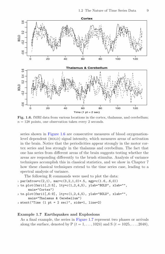
Fig. 1.6. fMRI data from various locations in the cortex, thalamus, and cerebellum;n = 128 points, one observation taken every 2 seconds.
series shown in Figure 1.6 are consecutive measures of blood oxygenation-level dependent (bold) signal intensity, which measures areas of activationin the brain. Notice that the periodicities appear strongly in the motor cor-tex series and less strongly in the thalamus and cerebellum. The fact thatone has series from different areas of the brain suggests testing whether theareas are responding differently to the brush stimulus. Analysis of variancetechniques accomplish this in classical statistics, and we show in Chapter 7how these classical techniques extend to the time series case, leading to aspectral analysis of variance.
The following R commands were used to plot the data:1 par(mfrow=c(2,1), mar=c(3,2,1,0)+.5, mgp=c(1.6,.6,0))
2 ts.plot(fmri1[,2:5], lty=c(1,2,4,5), ylab="BOLD", xlab="",
main="Cortex")
3 ts.plot(fmri1[,6:9], lty=c(1,2,4,5), ylab="BOLD", xlab="",
main="Thalamus & Cerebellum")
4 mtext("Time (1 pt = 2 sec)", side=1, line=2)
Example 1.7 Earthquakes and Explosions
As a final example, the series in Figure 1.7 represent two phases or arrivalsalong the surface, denoted by P (t = 1, . . . , 1024) and S (t = 1025, . . . , 2048),

10 1 Characteristics of Time Series
Earthquake
Time
EQ5
0 500 1000 1500 2000
−0.4
0.0
0.4
Explosion
Time
EXP6
0 500 1000 1500 2000
−0.4
0.0
0.4
Fig. 1.7. Arrival phases from an earthquake (top) and explosion (bottom) at 40points per second.
at a seismic recording station. The recording instruments in Scandinavia areobserving earthquakes and mining explosions with one of each shown in Fig-ure 1.7. The general problem of interest is in distinguishing or discriminatingbetween waveforms generated by earthquakes and those generated by explo-sions. Features that may be important are the rough amplitude ratios of thefirst phase P to the second phase S, which tend to be smaller for earth-quakes than for explosions. In the case of the two events in Figure 1.7, theratio of maximum amplitudes appears to be somewhat less than .5 for theearthquake and about 1 for the explosion. Otherwise, note a subtle differ-ence exists in the periodic nature of the S phase for the earthquake. We canagain think about spectral analysis of variance for testing the equality of theperiodic components of earthquakes and explosions. We would also like to beable to classify future P and S components from events of unknown origin,leading to the time series discriminant analysis developed in Chapter 7.
To plot the data as in this example, use the following commands in R:1 par(mfrow=c(2,1))
2 plot(EQ5, main="Earthquake")
3 plot(EXP6, main="Explosion")

1.3 Time Series Statistical Models 11
1.3 Time Series Statistical Models
The primary objective of time series analysis is to develop mathematical mod-els that provide plausible descriptions for sample data, like that encounteredin the previous section. In order to provide a statistical setting for describingthe character of data that seemingly fluctuate in a random fashion over time,we assume a time series can be defined as a collection of random variables in-dexed according to the order they are obtained in time. For example, we mayconsider a time series as a sequence of random variables, x1, x2, x3, . . . , wherethe random variable x1 denotes the value taken by the series at the first timepoint, the variable x2 denotes the value for the second time period, x3 denotesthe value for the third time period, and so on. In general, a collection of ran-dom variables, {xt}, indexed by t is referred to as a stochastic process. In thistext, t will typically be discrete and vary over the integers t = 0,±1,±2, ...,or some subset of the integers. The observed values of a stochastic process arereferred to as a realization of the stochastic process. Because it will be clearfrom the context of our discussions, we use the term time series whether weare referring generically to the process or to a particular realization and makeno notational distinction between the two concepts.
It is conventional to display a sample time series graphically by plottingthe values of the random variables on the vertical axis, or ordinate, withthe time scale as the abscissa. It is usually convenient to connect the valuesat adjacent time periods to reconstruct visually some original hypotheticalcontinuous time series that might have produced these values as a discretesample. Many of the series discussed in the previous section, for example,could have been observed at any continuous point in time and are conceptuallymore properly treated as continuous time series. The approximation of theseseries by discrete time parameter series sampled at equally spaced pointsin time is simply an acknowledgment that sampled data will, for the mostpart, be discrete because of restrictions inherent in the method of collection.Furthermore, the analysis techniques are then feasible using computers, whichare limited to digital computations. Theoretical developments also rest on theidea that a continuous parameter time series should be specified in terms offinite-dimensional distribution functions defined over a finite number of pointsin time. This is not to say that the selection of the sampling interval or rateis not an extremely important consideration. The appearance of data can bechanged completely by adopting an insufficient sampling rate. We have allseen wagon wheels in movies appear to be turning backwards because of theinsufficient number of frames sampled by the camera. This phenomenon leadsto a distortion called aliasing (see §4.2).
The fundamental visual characteristic distinguishing the different seriesshown in Examples 1.1–1.7 is their differing degrees of smoothness. One pos-sible explanation for this smoothness is that it is being induced by the suppo-sition that adjacent points in time are correlated, so the value of the series attime t, say, xt, depends in some way on the past values xt−1, xt−2, . . .. This
12 1 Characteristics of Time Series
model expresses a fundamental way in which we might think about gener-ating realistic-looking time series. To begin to develop an approach to usingcollections of random variables to model time series, consider Example 1.8.
Example 1.8 White Noise
A simple kind of generated series might be a collection of uncorrelated ran-dom variables, wt, with mean 0 and finite variance σ2
w. The time seriesgenerated from uncorrelated variables is used as a model for noise in en-gineering applications, where it is called white noise; we shall sometimesdenote this process as wt ∼ wn(0, σ2
w). The designation white originatesfrom the analogy with white light and indicates that all possible periodicoscillations are present with equal strength.
We will, at times, also require the noise to be independent and identicallydistributed (iid) random variables with mean 0 and variance σ2
w. We shalldistinguish this case by saying white independent noise, or by writing wt ∼iid(0, σ2
w). A particularly useful white noise series is Gaussian white noise,wherein the wt are independent normal random variables, with mean 0 andvariance σ2
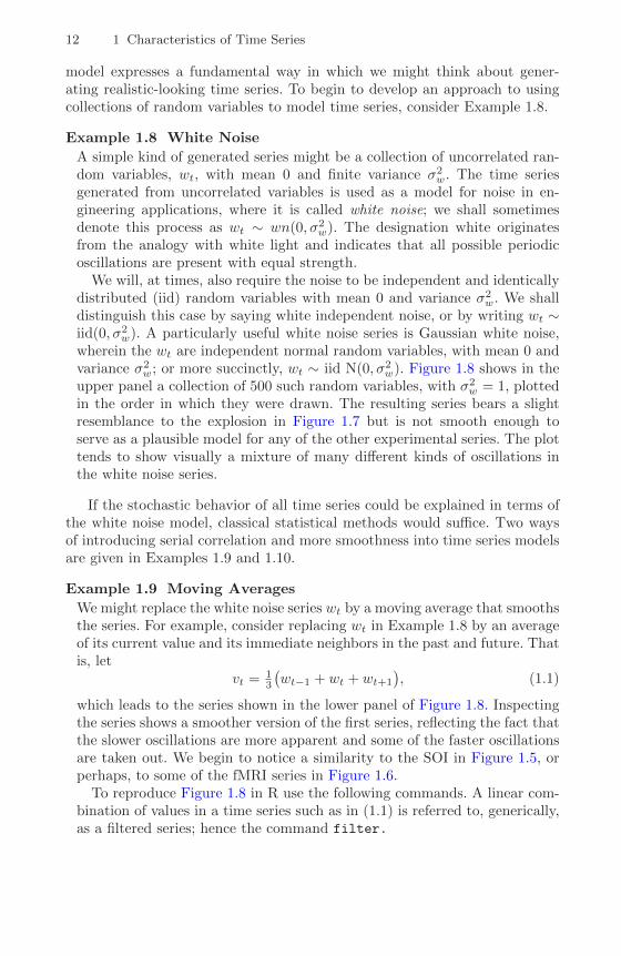
w; or more succinctly, wt ∼ iid N(0, σ2w). Figure 1.8 shows in the
upper panel a collection of 500 such random variables, with σ2w = 1, plotted
in the order in which they were drawn. The resulting series bears a slightresemblance to the explosion in Figure 1.7 but is not smooth enough toserve as a plausible model for any of the other experimental series. The plottends to show visually a mixture of many different kinds of oscillations inthe white noise series.
If the stochastic behavior of all time series could be explained in terms ofthe white noise model, classical statistical methods would suffice. Two waysof introducing serial correlation and more smoothness into time series modelsare given in Examples 1.9 and 1.10.
Example 1.9 Moving Averages
We might replace the white noise series wt by a moving average that smoothsthe series. For example, consider replacing wt in Example 1.8 by an averageof its current value and its immediate neighbors in the past and future. Thatis, let
vt = 13
(wt−1 + wt + wt+1
), (1.1)
which leads to the series shown in the lower panel of Figure 1.8. Inspectingthe series shows a smoother version of the first series, reflecting the fact thatthe slower oscillations are more apparent and some of the faster oscillationsare taken out. We begin to notice a similarity to the SOI in Figure 1.5, orperhaps, to some of the fMRI series in Figure 1.6.
To reproduce Figure 1.8 in R use the following commands. A linear com-bination of values in a time series such as in (1.1) is referred to, generically,as a filtered series; hence the command filter.

1.3 Time Series Statistical Models 13
white noise
Time
w
0 100 200 300 400 500
−3−1
01
2
moving average
v
0 100 200 300 400 500
−1.5
−0.5
0.5
1.5
Fig. 1.8. Gaussian white noise series (top) and three-point moving average of theGaussian white noise series (bottom).
1 w = rnorm(500,0,1) # 500 N(0,1) variates
2 v = filter(w, sides=2, rep(1/3,3)) # moving average
3 par(mfrow=c(2,1))
4 plot.ts(w, main="white noise")
5 plot.ts(v, main="moving average")
The speech series in Figure 1.3 and the Recruitment series in Figure 1.5,as well as some of the MRI series in Figure 1.6, differ from the moving averageseries because one particular kind of oscillatory behavior seems to predom-inate, producing a sinusoidal type of behavior. A number of methods existfor generating series with this quasi-periodic behavior; we illustrate a popularone based on the autoregressive model considered in Chapter 3.
Example 1.10 Autoregressions
Suppose we consider the white noise series wt of Example 1.8 as input andcalculate the output using the second-order equation
xt = xt−1 − .9xt−2 + wt (1.2)
successively for t = 1, 2, . . . , 500. Equation (1.2) represents a regression orprediction of the current value xt of a time series as a function of the pasttwo values of the series, and, hence, the term autoregression is suggested
14 1 Characteristics of Time Series
autoregressionx
0 100 200 300 400 500
−6−4
−20
24
6
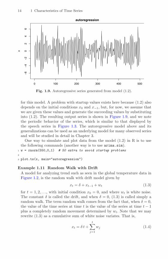
Fig. 1.9. Autoregressive series generated from model (1.2).
for this model. A problem with startup values exists here because (1.2) alsodepends on the initial conditions x0 and x−1, but, for now, we assume thatwe are given these values and generate the succeeding values by substitutinginto (1.2). The resulting output series is shown in Figure 1.9, and we notethe periodic behavior of the series, which is similar to that displayed bythe speech series in Figure 1.3. The autoregressive model above and itsgeneralizations can be used as an underlying model for many observed seriesand will be studied in detail in Chapter 3.
One way to simulate and plot data from the model (1.2) in R is to usethe following commands (another way is to use arima.sim).
1 w = rnorm(550,0,1) # 50 extra to avoid startup problems
2 x = filter(w, filter=c(1,-.9), method="recursive")[-(1:50)]
3 plot.ts(x, main="autoregression")
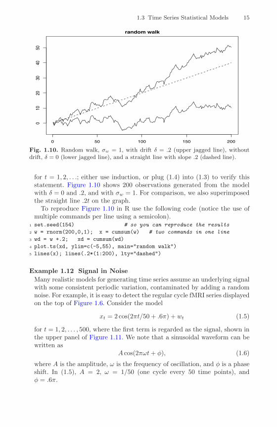
Example 1.11 Random Walk with Drift
A model for analyzing trend such as seen in the global temperature data inFigure 1.2, is the random walk with drift model given by
xt = δ + xt−1 + wt (1.3)
for t = 1, 2, . . ., with initial condition x0 = 0, and where wt is white noise.The constant δ is called the drift, and when δ = 0, (1.3) is called simply arandom walk. The term random walk comes from the fact that, when δ = 0,the value of the time series at time t is the value of the series at time t− 1plus a completely random movement determined by wt. Note that we mayrewrite (1.3) as a cumulative sum of white noise variates. That is,
xt = δ t+
t∑j=1
wj (1.4)
1.3 Time Series Statistical Models 15
random walk
0 50 100 150 200
010
2030
4050
Fig. 1.10. Random walk, σw = 1, with drift δ = .2 (upper jagged line), withoutdrift, δ = 0 (lower jagged line), and a straight line with slope .2 (dashed line).
for t = 1, 2, . . .; either use induction, or plug (1.4) into (1.3) to verify thisstatement. Figure 1.10 shows 200 observations generated from the modelwith δ = 0 and .2, and with σw = 1. For comparison, we also superimposedthe straight line .2t on the graph.
To reproduce Figure 1.10 in R use the following code (notice the use ofmultiple commands per line using a semicolon).
1 set.seed(154) # so you can reproduce the results
2 w = rnorm(200,0,1); x = cumsum(w) # two commands in one line
3 wd = w +.2; xd = cumsum(wd)
4 plot.ts(xd, ylim=c(-5,55), main="random walk")
5 lines(x); lines(.2*(1:200), lty="dashed")
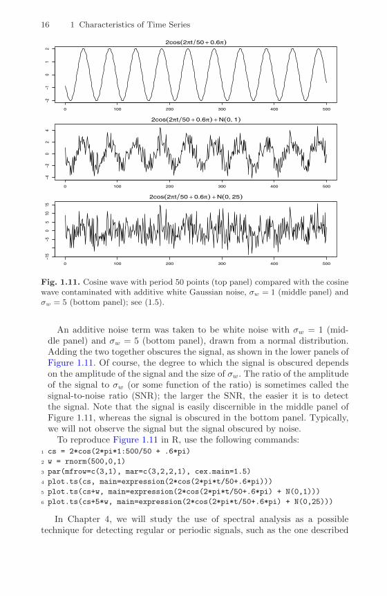
Example 1.12 Signal in Noise
Many realistic models for generating time series assume an underlying signalwith some consistent periodic variation, contaminated by adding a randomnoise. For example, it is easy to detect the regular cycle fMRI series displayedon the top of Figure 1.6. Consider the model
xt = 2 cos(2πt/50 + .6π) + wt (1.5)
for t = 1, 2, . . . , 500, where the first term is regarded as the signal, shown inthe upper panel of Figure 1.11. We note that a sinusoidal waveform can bewritten as
A cos(2πωt+ φ), (1.6)
where A is the amplitude, ω is the frequency of oscillation, and φ is a phaseshift. In (1.5), A = 2, ω = 1/50 (one cycle every 50 time points), andφ = .6π.
16 1 Characteristics of Time Series
2cos2t 50 0.6
0 100 200 300 400 500
−2−1
01
2
2cos2t 50 0.6 N01
0 100 200 300 400 500
−4−2
02
4
2cos2t 50 0.6 N025
0 100 200 300 400 500
−15
−50
510
15
Fig. 1.11. Cosine wave with period 50 points (top panel) compared with the cosinewave contaminated with additive white Gaussian noise, σw = 1 (middle panel) andσw = 5 (bottom panel); see (1.5).
An additive noise term was taken to be white noise with σw = 1 (mid-dle panel) and σw = 5 (bottom panel), drawn from a normal distribution.Adding the two together obscures the signal, as shown in the lower panels ofFigure 1.11. Of course, the degree to which the signal is obscured dependson the amplitude of the signal and the size of σw. The ratio of the amplitudeof the signal to σw (or some function of the ratio) is sometimes called thesignal-to-noise ratio (SNR); the larger the SNR, the easier it is to detectthe signal. Note that the signal is easily discernible in the middle panel ofFigure 1.11, whereas the signal is obscured in the bottom panel. Typically,we will not observe the signal but the signal obscured by noise.
To reproduce Figure 1.11 in R, use the following commands:1 cs = 2*cos(2*pi*1:500/50 + .6*pi)
2 w = rnorm(500,0,1)
3 par(mfrow=c(3,1), mar=c(3,2,2,1), cex.main=1.5)
4 plot.ts(cs, main=expression(2*cos(2*pi*t/50+.6*pi)))
5 plot.ts(cs+w, main=expression(2*cos(2*pi*t/50+.6*pi) + N(0,1)))
6 plot.ts(cs+5*w, main=expression(2*cos(2*pi*t/50+.6*pi) + N(0,25)))
In Chapter 4, we will study the use of spectral analysis as a possibletechnique for detecting regular or periodic signals, such as the one described

1.4Measures of Dependence 17
in Example 1.12. In general, we would emphasize the importance of simpleadditive models such as given above in the form
xt = st + vt, (1.7)
where st denotes some unknown signal and vt denotes a time series that maybe white or correlated over time. The problems of detecting a signal and thenin estimating or extracting the waveform of st are of great interest in manyareas of engineering and the physical and biological sciences. In economics,the underlying signal may be a trend or it may be a seasonal component of aseries. Models such as (1.7), where the signal has an autoregressive structure,form the motivation for the state-space model of Chapter 6.
In the above examples, we have tried to motivate the use of various com-binations of random variables emulating real time series data. Smoothnesscharacteristics of observed time series were introduced by combining the ran-dom variables in various ways. Averaging independent random variables overadjacent time points, as in Example 1.9, or looking at the output of differ-ence equations that respond to white noise inputs, as in Example 1.10, arecommon ways of generating correlated data. In the next section, we introducevarious theoretical measures used for describing how time series behave. Asis usual in statistics, the complete description involves the multivariate dis-tribution function of the jointly sampled values x1, x2, . . . , xn, whereas moreeconomical descriptions can be had in terms of the mean and autocorrelationfunctions. Because correlation is an essential feature of time series analysis, themost useful descriptive measures are those expressed in terms of covarianceand correlation functions.
1.4 Measures of Dependence: Autocorrelation andCross-Correlation
A complete description of a time series, observed as a collection of n randomvariables at arbitrary integer time points t1, t2, . . . , tn, for any positive integern, is provided by the joint distribution function, evaluated as the probabilitythat the values of the series are jointly less than the n constants, c1, c2, . . . , cn;i.e.,
F (c1, c2, . . . , cn) = P(xt1 ≤ c1, xt2 ≤ c2, . . . , xtn ≤ cn
). (1.8)
Unfortunately, the multidimensional distribution function cannot usually bewritten easily unless the random variables are jointly normal, in which casethe joint density has the well-known form displayed in (1.31).
Although the joint distribution function describes the data completely, itis an unwieldy tool for displaying and analyzing time series data. The dis-tribution function (1.8) must be evaluated as a function of n arguments, soany plotting of the corresponding multivariate density functions is virtuallyimpossible. The marginal distribution functions

18 1 Characteristics of Time Series
Ft(x) = P{xt ≤ x}
or the corresponding marginal density functions
ft(x) =∂Ft(x)
∂x,
when they exist, are often informative for examining the marginal behaviorof a series.2 Another informative marginal descriptive measure is the meanfunction.
Definition 1.1 The mean function is defined as
µxt = E(xt) =
∫ ∞−∞
xft(x) dx, (1.9)
provided it exists, where E denotes the usual expected value operator. Whenno confusion exists about which time series we are referring to, we will dropa subscript and write µxt as µt.
Example 1.13 Mean Function of a Moving Average Series
If wt denotes a white noise series, then µwt = E(wt) = 0 for all t. The topseries in Figure 1.8 reflects this, as the series clearly fluctuates around amean value of zero. Smoothing the series as in Example 1.9 does not changethe mean because we can write
µvt = E(vt) = 13 [E(wt−1) + E(wt) + E(wt+1)] = 0.
Example 1.14 Mean Function of a Random Walk with Drift
Consider the random walk with drift model given in (1.4),
xt = δ t+t∑
j=1
wj , t = 1, 2, . . . .
Because E(wt) = 0 for all t, and δ is a constant, we have
µxt = E(xt) = δ t+
t∑j=1
E(wj) = δ t
which is a straight line with slope δ. A realization of a random walk withdrift can be compared to its mean function in Figure 1.10.
2 If xt is Gaussian with mean µt and variance σ2t , abbreviated as xt ∼ N(µt, σ
2t ),
the marginal density is given by ft(x) =1
σt√
2πexp
{− 1
2σ2t
(x− µt)2}
.

1.4Measures of Dependence 19
Example 1.15 Mean Function of Signal Plus Noise
A great many practical applications depend on assuming the observed datahave been generated by a fixed signal waveform superimposed on a zero-mean noise process, leading to an additive signal model of the form (1.5). Itis clear, because the signal in (1.5) is a fixed function of time, we will have
µxt = E(xt) = E[2 cos(2πt/50 + .6π) + wt
]= 2 cos(2πt/50 + .6π) + E(wt)
= 2 cos(2πt/50 + .6π),
and the mean function is just the cosine wave.
The lack of independence between two adjacent values xs and xt can beassessed numerically, as in classical statistics, using the notions of covarianceand correlation. Assuming the variance of xt is finite, we have the followingdefinition.
Definition 1.2 The autocovariance function is defined as the second mo-ment product
γx(s, t) = cov(xs, xt) = E[(xs − µs)(xt − µt)], (1.10)
for all s and t. When no possible confusion exists about which time series weare referring to, we will drop the subscript and write γx(s, t) as γ(s, t).
Note that γx(s, t) = γx(t, s) for all time points s and t. The autocovariancemeasures the linear dependence between two points on the same series ob-served at different times. Very smooth series exhibit autocovariance functionsthat stay large even when the t and s are far apart, whereas choppy series tendto have autocovariance functions that are nearly zero for large separations.The autocovariance (1.10) is the average cross-product relative to the jointdistribution F (xs, xt). Recall from classical statistics that if γx(s, t) = 0, xsand xt are not linearly related, but there still may be some dependence struc-ture between them. If, however, xs and xt are bivariate normal, γx(s, t) = 0ensures their independence. It is clear that, for s = t, the autocovariancereduces to the (assumed finite) variance, because
γx(t, t) = E[(xt − µt)2] = var(xt). (1.11)
Example 1.16 Autocovariance of White Noise
The white noise series wt has E(wt) = 0 and
γw(s, t) = cov(ws, wt) =
{σ2w s = t,
0 s 6= t.(1.12)
A realization of white noise with σ2w = 1 is shown in the top panel of
Figure 1.8.

20 1 Characteristics of Time Series
Example 1.17 Autocovariance of a Moving Average
Consider applying a three-point moving average to the white noise series wtof the previous example as in Example 1.9. In this case,
γv(s, t) = cov(vs, vt) = cov{
13 (ws−1 + ws + ws+1) , 13 (wt−1 + wt + wt+1)
}.
When s = t we have3
γv(t, t) = 19cov{(wt−1 + wt + wt+1), (wt−1 + wt + wt+1)}
= 19 [cov(wt−1, wt−1) + cov(wt, wt) + cov(wt+1, wt+1)]
= 39σ
2w.
When s = t+ 1,
γv(t+ 1, t) = 19cov{(wt + wt+1 + wt+2), (wt−1 + wt + wt+1)}
= 19 [cov(wt, wt) + cov(wt+1, wt+1)]
= 29σ
2w,
using (1.12). Similar computations give γv(t − 1, t) = 2σ2w/9, γv(t + 2, t) =
γv(t− 2, t) = σ2w/9, and 0 when |t− s| > 2. We summarize the values for all
s and t as
γv(s, t) =
39σ
2w s = t,
29σ
2w |s− t| = 1,
19σ
2w |s− t| = 2,
0 |s− t| > 2.
(1.13)
Example 1.17 shows clearly that the smoothing operation introduces acovariance function that decreases as the separation between the two timepoints increases and disappears completely when the time points are separatedby three or more time points. This particular autocovariance is interestingbecause it only depends on the time separation or lag and not on the absolutelocation of the points along the series. We shall see later that this dependencesuggests a mathematical model for the concept of weak stationarity.
Example 1.18 Autocovariance of a Random Walk
For the random walk model, xt =∑tj=1 wj , we have
γx(s, t) = cov(xs, xt) = cov
s∑j=1
wj ,
t∑k=1
wk
= min{s, t}σ2w,
because the wt are uncorrelated random variables. Note that, as opposedto the previous examples, the autocovariance function of a random walk
3 If the random variables U =∑mj=1 ajXj and V =
∑rk=1 bkYk are linear com-
binations of random variables {Xj} and {Yk}, respectively, then cov(U, V ) =∑mj=1
∑rk=1 ajbkcov(Xj , Yk). Furthermore, var(U) = cov(U,U).
1.4Measures of Dependence 21
depends on the particular time values s and t, and not on the time separationor lag. Also, notice that the variance of the random walk, var(xt) = γx(t, t) =t σ2
w, increases without bound as time t increases. The effect of this varianceincrease can be seen in Figure 1.10 where the processes start to move awayfrom their mean functions δ t (note that δ = 0 and .2 in that example).
As in classical statistics, it is more convenient to deal with a measure ofassociation between −1 and 1, and this leads to the following definition.
Definition 1.3 The autocorrelation function (ACF) is defined as
ρ(s, t) =γ(s, t)√
γ(s, s)γ(t, t). (1.14)
The ACF measures the linear predictability of the series at time t, say xt,using only the value xs. We can show easily that −1 ≤ ρ(s, t) ≤ 1 using theCauchy–Schwarz inequality.4 If we can predict xt perfectly from xs througha linear relationship, xt = β0 + β1xs, then the correlation will be +1 whenβ1 > 0, and −1 when β1 < 0. Hence, we have a rough measure of the abilityto forecast the series at time t from the value at time s.
Often, we would like to measure the predictability of another series yt fromthe series xs. Assuming both series have finite variances, we have the followingdefinition.
Definition 1.4 The cross-covariance function between two series, xt andyt, is
γxy(s, t) = cov(xs, yt) = E[(xs − µxs)(yt − µyt)]. (1.15)
There is also a scaled version of the cross-covariance function.
Definition 1.5 The cross-correlation function (CCF) is given by
ρxy(s, t) =γxy(s, t)√
γx(s, s)γy(t, t). (1.16)
We may easily extend the above ideas to the case of more than two series,say, xt1, xt2, . . . , xtr; that is, multivariate time series with r components. Forexample, the extension of (1.10) in this case is
γjk(s, t) = E[(xsj − µsj)(xtk − µtk)] j, k = 1, 2, . . . , r. (1.17)
In the definitions above, the autocovariance and cross-covariance functionsmay change as one moves along the series because the values depend on both s
4 The Cauchy–Schwarz inequality implies |γ(s, t)|2 ≤ γ(s, s)γ(t, t).
22 1 Characteristics of Time Series
and t, the locations of the points in time. In Example 1.17, the autocovariancefunction depends on the separation of xs and xt, say, h = |s− t|, and not onwhere the points are located in time. As long as the points are separated byh units, the location of the two points does not matter. This notion, calledweak stationarity, when the mean is constant, is fundamental in allowing usto analyze sample time series data when only a single series is available.
1.5 Stationary Time Series
The preceding definitions of the mean and autocovariance functions are com-pletely general. Although we have not made any special assumptions aboutthe behavior of the time series, many of the preceding examples have hintedthat a sort of regularity may exist over time in the behavior of a time series.We introduce the notion of regularity using a concept called stationarity.
Definition 1.6 A strictly stationary time series is one for which the prob-abilistic behavior of every collection of values
{xt1 , xt2 , . . . , xtk}
is identical to that of the time shifted set
{xt1+h, xt2+h, . . . , xtk+h}.
That is,
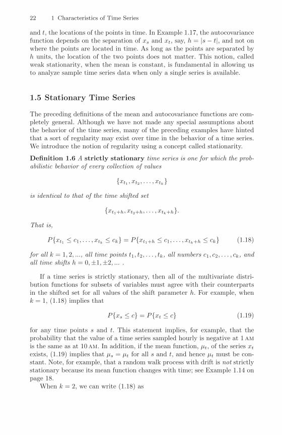
P{xt1 ≤ c1, . . . , xtk ≤ ck} = P{xt1+h ≤ c1, . . . , xtk+h ≤ ck} (1.18)
for all k = 1, 2, ..., all time points t1, t2, . . . , tk, all numbers c1, c2, . . . , ck, andall time shifts h = 0,±1,±2, ... .
If a time series is strictly stationary, then all of the multivariate distri-bution functions for subsets of variables must agree with their counterpartsin the shifted set for all values of the shift parameter h. For example, whenk = 1, (1.18) implies that
P{xs ≤ c} = P{xt ≤ c} (1.19)
for any time points s and t. This statement implies, for example, that theprobability that the value of a time series sampled hourly is negative at 1amis the same as at 10am. In addition, if the mean function, µt, of the series xtexists, (1.19) implies that µs = µt for all s and t, and hence µt must be con-stant. Note, for example, that a random walk process with drift is not strictlystationary because its mean function changes with time; see Example 1.14 onpage 18.
When k = 2, we can write (1.18) as

1.5 Stationary Time Series 23
P{xs ≤ c1, xt ≤ c2} = P{xs+h ≤ c1, xt+h ≤ c2} (1.20)
for any time points s and t and shift h. Thus, if the variance function of theprocess exists, (1.20) implies that the autocovariance function of the series xtsatisfies
γ(s, t) = γ(s+ h, t+ h)
for all s and t and h. We may interpret this result by saying the autocovariancefunction of the process depends only on the time difference between s and t,and not on the actual times.
The version of stationarity in Definition 1.6 is too strong for most appli-cations. Moreover, it is difficult to assess strict stationarity from a single dataset. Rather than imposing conditions on all possible distributions of a timeseries, we will use a milder version that imposes conditions only on the firsttwo moments of the series. We now have the following definition.
Definition 1.7 A weakly stationary time series, xt, is a finite varianceprocess such that
(i) the mean value function, µt, defined in (1.9) is constant and does notdepend on time t, and
(ii) the autocovariance function, γ(s, t), defined in (1.10) depends on s andt only through their difference |s− t|.
Henceforth, we will use the term stationary to mean weakly stationary; if aprocess is stationary in the strict sense, we will use the term strictly stationary.
It should be clear from the discussion of strict stationarity following Defini-tion 1.6 that a strictly stationary, finite variance, time series is also stationary.The converse is not true unless there are further conditions. One importantcase where stationarity implies strict stationarity is if the time series is Gaus-sian [meaning all finite distributions, (1.18), of the series are Gaussian]. Wewill make this concept more precise at the end of this section.
Because the mean function, E(xt) = µt, of a stationary time series isindependent of time t, we will write
µt = µ. (1.21)
Also, because the autocovariance function, γ(s, t), of a stationary time series,xt, depends on s and t only through their difference |s− t|, we may simplifythe notation. Let s = t+ h, where h represents the time shift or lag. Then
γ(t+ h, t) = cov(xt+h, xt) = cov(xh, x0) = γ(h, 0)
because the time difference between times t + h and t is the same as thetime difference between times h and 0. Thus, the autocovariance function ofa stationary time series does not depend on the time argument t. Henceforth,for convenience, we will drop the second argument of γ(h, 0).

24 1 Characteristics of Time Series
−4 −2 0 2 4
0.00
0.15
0.30
Lag
ACov
F
Fig. 1.12. Autocovariance function of a three-point moving average.
Definition 1.8 The autocovariance function of a stationary time se-ries will be written as
γ(h) = cov(xt+h, xt) = E[(xt+h − µ)(xt − µ)]. (1.22)
Definition 1.9 The autocorrelation function (ACF) of a stationarytime series will be written using (1.14) as
ρ(h) =γ(t+ h, t)√
γ(t+ h, t+ h)γ(t, t)=γ(h)
γ(0). (1.23)
The Cauchy–Schwarz inequality shows again that −1 ≤ ρ(h) ≤ 1 for allh, enabling one to assess the relative importance of a given autocorrelationvalue by comparing with the extreme values −1 and 1.
Example 1.19 Stationarity of White Noise
The mean and autocovariance functions of the white noise series discussedin Examples 1.8 and 1.16 are easily evaluated as µwt = 0 and
γw(h) = cov(wt+h, wt) =
{σ2w h = 0,
0 h 6= 0.
Thus, white noise satisfies the conditions of Definition 1.7 and is weaklystationary or stationary. If the white noise variates are also normally dis-tributed or Gaussian, the series is also strictly stationary, as can be seen byevaluating (1.18) using the fact that the noise would also be iid.
Example 1.20 Stationarity of a Moving Average
The three-point moving average process of Example 1.9 is stationary be-cause, from Examples 1.13 and 1.17, the mean and autocovariance functionsµvt = 0, and

1.5 Stationary Time Series 25
γv(h) =
39σ
2w h = 0,
29σ
2w h = ±1,
19σ
2w h = ±2,
0 |h| > 2
are independent of time t, satisfying the conditions of Definition 1.7. Fig-ure 1.12 shows a plot of the autocovariance as a function of lag h withσ2w = 1. Interestingly, the autocovariance function is symmetric about lag
zero and decays as a function of lag.
The autocovariance function of a stationary process has several usefulproperties (also, see Problem 1.25). First, the value at h = 0, namely
γ(0) = E[(xt − µ)2] (1.24)
is the variance of the time series; note that the Cauchy–Schwarz inequalityimplies
|γ(h)| ≤ γ(0).
A final useful property, noted in the previous example, is that the autoco-variance function of a stationary series is symmetric around the origin; thatis,
γ(h) = γ(−h) (1.25)
for all h. This property follows because shifting the series by h means that
γ(h) = γ(t+ h− t)= E[(xt+h − µ)(xt − µ)]= E[(xt − µ)(xt+h − µ)]= γ(t− (t+ h))= γ(−h),
which shows how to use the notation as well as proving the result.When several series are available, a notion of stationarity still applies with
additional conditions.
Definition 1.10 Two time series, say, xt and yt, are said to be jointly sta-tionary if they are each stationary, and the cross-covariance function
γxy(h) = cov(xt+h, yt) = E[(xt+h − µx)(yt − µy)] (1.26)
is a function only of lag h.
Definition 1.11 The cross-correlation function (CCF) of jointly station-ary time series xt and yt is defined as
ρxy(h) =γxy(h)√γx(0)γy(0)
. (1.27)

26 1 Characteristics of Time Series
Again, we have the result −1 ≤ ρxy(h) ≤ 1 which enables comparison withthe extreme values −1 and 1 when looking at the relation between xt+h andyt. The cross-correlation function is not generally symmetric about zero [i.e.,typically ρxy(h) 6= ρxy(−h)]; however, it is the case that
ρxy(h) = ρyx(−h), (1.28)
which can be shown by manipulations similar to those used to show (1.25).
Example 1.21 Joint Stationarity
Consider the two series, xt and yt, formed from the sum and difference oftwo successive values of a white noise process, say,
xt = wt + wt−1
andyt = wt − wt−1,
where wt are independent random variables with zero means and varianceσ2w. It is easy to show that γx(0) = γy(0) = 2σ2
w and γx(1) = γx(−1) =σ2w, γy(1) = γy(−1) = −σ2
w. Also,
γxy(1) = cov(xt+1, yt) = cov(wt+1 + wt, wt − wt−1) = σ2w
because only one term is nonzero (recall footnote 3 on page 20). Similarly,γxy(0) = 0, γxy(−1) = −σ2
w. We obtain, using (1.27),
ρxy(h) =
0 h = 0,
1/2 h = 1,
−1/2 h = −1,
0 |h| ≥ 2.
Clearly, the autocovariance and cross-covariance functions depend only onthe lag separation, h, so the series are jointly stationary.
Example 1.22 Prediction Using Cross-Correlation
As a simple example of cross-correlation, consider the problem of determin-ing possible leading or lagging relations between two series xt and yt. If themodel
yt = Axt−` + wt
holds, the series xt is said to lead yt for ` > 0 and is said to lag yt for ` < 0.Hence, the analysis of leading and lagging relations might be important inpredicting the value of yt from xt. Assuming, for convenience, that xt andyt have zero means, and the noise wt is uncorrelated with the xt series, thecross-covariance function can be computed as

1.5 Stationary Time Series 27
γyx(h) = cov(yt+h, xt) = cov(Axt+h−` + wt+h, xt)
= cov(Axt+h−`, xt) = Aγx(h− `).
The cross-covariance function will look like the autocovariance of the inputseries xt, with a peak on the positive side if xt leads yt and a peak on thenegative side if xt lags yt.
The concept of weak stationarity forms the basis for much of the analy-sis performed with time series. The fundamental properties of the mean andautocovariance functions (1.21) and (1.22) are satisfied by many theoreticalmodels that appear to generate plausible sample realizations. In Examples 1.9and 1.10, two series were generated that produced stationary looking realiza-tions, and in Example 1.20, we showed that the series in Example 1.9 was, infact, weakly stationary. Both examples are special cases of the so-called linearprocess.
Definition 1.12 A linear process, xt, is defined to be a linear combinationof white noise variates wt, and is given by
xt = µ+∞∑
j=−∞ψjwt−j ,
∞∑j=−∞
|ψj | <∞. (1.29)
For the linear process (see Problem 1.11), we may show that the autoco-variance function is given by
γ(h) = σ2w
∞∑j=−∞
ψj+hψj (1.30)
for h ≥ 0; recall that γ(−h) = γ(h). This method exhibits the autocovariancefunction of the process in terms of the lagged products of the coefficients. Notethat, for Example 1.9, we have ψ0 = ψ−1 = ψ1 = 1/3 and the result in Ex-ample 1.20 comes out immediately. The autoregressive series in Example 1.10can also be put in this form, as can the general autoregressive moving averageprocesses considered in Chapter 3.
Finally, as previously mentioned, an important case in which a weaklystationary series is also strictly stationary is the normal or Gaussian series.
Definition 1.13 A process, {xt}, is said to be a Gaussian process if then-dimensional vectors xxx = (xt1 , xt2 , . . . , xtn)′, for every collection of timepoints t1, t2, . . . , tn, and every positive integer n, have a multivariate normaldistribution.
Defining the n × 1 mean vector E(xxx) ≡ µµµ = (µt1 , µt2 , . . . , µtn)′ and then× n covariance matrix as var(xxx) ≡ Γ = {γ(ti, tj); i, j = 1, . . . , n}, which is

28 1 Characteristics of Time Series
assumed to be positive definite, the multivariate normal density function canbe written as
f(xxx) = (2π)−n/2|Γ |−1/2 exp
{−1
2(xxx− µµµ)′Γ−1(xxx− µµµ)
}, (1.31)
where |·| denotes the determinant. This distribution forms the basis for solvingproblems involving statistical inference for time series. If a Gaussian timeseries, {xt}, is weakly stationary, then µt = µ and γ(ti, tj) = γ(|ti − tj |),so that the vector µµµ and the matrix Γ are independent of time. These factsimply that all the finite distributions, (1.31), of the series {xt} depend onlyon time lag and not on the actual times, and hence the series must be strictlystationary.
1.6 Estimation of Correlation
Although the theoretical autocorrelation and cross-correlation functions areuseful for describing the properties of certain hypothesized models, most ofthe analyses must be performed using sampled data. This limitation meansthe sampled points x1, x2, . . . , xn only are available for estimating the mean,autocovariance, and autocorrelation functions. From the point of view of clas-sical statistics, this poses a problem because we will typically not have iidcopies of xt that are available for estimating the covariance and correlationfunctions. In the usual situation with only one realization, however, the as-sumption of stationarity becomes critical. Somehow, we must use averagesover this single realization to estimate the population means and covariancefunctions.
Accordingly, if a time series is stationary, the mean function (1.21) µt = µis constant so that we can estimate it by the sample mean,
x =1
n
n∑t=1
xt. (1.32)
The standard error of the estimate is the square root of var(x), which can becomputed using first principles (recall footnote 3 on page 20), and is given by
var(x) = var
(1
n
n∑t=1
xt
)=
1
n2cov
(n∑t=1
xt,
n∑s=1
xs
)
=1
n2
(nγx(0) + (n− 1)γx(1) + (n− 2)γx(2) + · · ·+ γx(n− 1)
+ (n− 1)γx(−1) + (n− 2)γx(−2) + · · ·+ γx(1− n))
=1
n
n∑h=−n
(1− |h|
n
)γx(h). (1.33)

1.6 Estimation of Correlation 29
If the process is white noise, (1.33) reduces to the familiar σ2x/n recalling that
γx(0) = σ2x. Note that, in the case of dependence, the standard error of x may
be smaller or larger than the white noise case depending on the nature of thecorrelation structure (see Problem 1.19)
The theoretical autocovariance function, (1.22), is estimated by the sampleautocovariance function defined as follows.
Definition 1.14 The sample autocovariance function is defined as
γ(h) = n−1n−h∑t=1
(xt+h − x)(xt − x), (1.34)
with γ(−h) = γ(h) for h = 0, 1, . . . , n− 1.
The sum in (1.34) runs over a restricted range because xt+h is not availablefor t + h > n. The estimator in (1.34) is preferred to the one that would beobtained by dividing by n−h because (1.34) is a non-negative definite function.The autocovariance function, γ(h), of a stationary process is non-negativedefinite (see Problem 1.25) ensuring that variances of linear combinations ofthe variates xt will never be negative. And, because var(a1xt1 + · · ·+ anxtn)is never negative, the estimate of that variance should also be non-negative.The estimator in (1.34) guarantees this result, but no such guarantee exists ifwe divide by n−h; this is explored further in Problem 1.25. Note that neitherdividing by n nor n− h in (1.34) yields an unbiased estimator of γ(h).
Definition 1.15 The sample autocorrelation function is defined, analo-gously to (1.23), as
ρ(h) =γ(h)
γ(0). (1.35)
The sample autocorrelation function has a sampling distribution that al-lows us to assess whether the data comes from a completely random or whiteseries or whether correlations are statistically significant at some lags.
Property 1.1 Large-Sample Distribution of the ACFUnder general conditions,5 if xt is white noise, then for n large, the sample
ACF, ρx(h), for h = 1, 2, . . . ,H, where H is fixed but arbitrary, is approxi-mately normally distributed with zero mean and standard deviation given by
σρx(h) =1√n. (1.36)
5 The general conditions are that xt is iid with finite fourth moment. A sufficientcondition for this to hold is that xt is white Gaussian noise. Precise details aregiven in Theorem A.7 in Appendix A.

30 1 Characteristics of Time Series
Based on the previous result, we obtain a rough method of assessingwhether peaks in ρ(h) are significant by determining whether the observedpeak is outside the interval ±2/
√n (or plus/minus two standard errors); for
a white noise sequence, approximately 95% of the sample ACFs should bewithin these limits. The applications of this property develop because manystatistical modeling procedures depend on reducing a time series to a whitenoise series using various kinds of transformations. After such a procedure isapplied, the plotted ACFs of the residuals should then lie roughly within thelimits given above.
Definition 1.16 The estimators for the cross-covariance function, γxy(h), asgiven in (1.26) and the cross-correlation, ρxy(h), in (1.27) are given, respec-tively, by the sample cross-covariance function
γxy(h) = n−1n−h∑t=1
(xt+h − x)(yt − y), (1.37)
where γxy(−h) = γyx(h) determines the function for negative lags, and thesample cross-correlation function
ρxy(h) =γxy(h)√γx(0)γy(0)
. (1.38)
The sample cross-correlation function can be examined graphically as afunction of lag h to search for leading or lagging relations in the data usingthe property mentioned in Example 1.22 for the theoretical cross-covariancefunction. Because −1 ≤ ρxy(h) ≤ 1, the practical importance of peaks canbe assessed by comparing their magnitudes with their theoretical maximumvalues. Furthermore, for xt and yt independent linear processes of the form(1.29), we have the following property.
Property 1.2 Large-Sample Distribution of Cross-CorrelationUnder Independence
The large sample distribution of ρxy(h) is normal with mean zero and
σρxy =1√n
(1.39)
if at least one of the processes is independent white noise (see Theorem A.8in Appendix A).
Example 1.23 A Simulated Time Series
To give an example of the procedure for calculating numerically the auto-covariance and cross-covariance functions, consider a contrived set of data

1.6 Estimation of Correlation 31
Table 1.1. Sample Realization of the Contrived Series yt
t 1 2 3 4 5 6 7 8 9 10
Coin H H T H T T T H T Hxt 1 1 −1 1 −1 −1 −1 1 −1 1yt 6.7 5.3 3.3 6.7 3.3 4.7 4.7 6.7 3.3 6.7
yt − y 1.56 .16 −1.84 1.56 −1.84 −.44 −.44 1.56 −1.84 1.56
generated by tossing a fair coin, letting xt = 1 when a head is obtained andxt = −1 when a tail is obtained. Construct yt as
yt = 5 + xt − .7xt−1. (1.40)
Table 1.1 shows sample realizations of the appropriate processes with x0 =−1 and n = 10.
The sample autocorrelation for the series yt can be calculated using (1.34)and (1.35) for h = 0, 1, 2, . . .. It is not necessary to calculate for negativevalues because of the symmetry. For example, for h = 3, the autocorrelationbecomes the ratio of
γy(3) = 110
7∑t=1
(yt+3 − y)(yt − y)
= 110
[(1.56)(1.56) + (−1.84)(.16) + (−.44)(−1.84) + (−.44)(1.56)
+ (1.56)(−1.84) + (−1.84)(−.44) + (1.56)(−.44)]
= −.048
toγy(0) = 1
10 [(1.56)2 + (.16)2 + · · ·+ (1.56)2] = 2.030
so that
ρy(3) =−.048
2.030= −.024.
The theoretical ACF can be obtained from the model (1.40) using the factthat the mean of xt is zero and the variance of xt is one. It can be shownthat
ρy(1) =−.7
1 + .72= −.47
and ρy(h) = 0 for |h| > 1 (Problem 1.24). Table 1.2 compares the theo-retical ACF with sample ACFs for a realization where n = 10 and anotherrealization where n = 100; we note the increased variability in the smallersize sample.
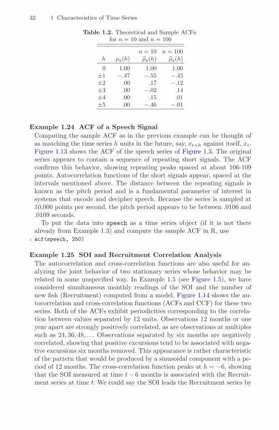
32 1 Characteristics of Time Series
Table 1.2. Theoretical and Sample ACFsfor n = 10 and n = 100
n = 10 n = 100h ρy(h) ρy(h) ρy(h)
0 1.00 1.00 1.00±1 −.47 −.55 −.45±2 .00 .17 −.12±3 .00 −.02 .14±4 .00 .15 .01±5 .00 −.46 −.01
Example 1.24 ACF of a Speech Signal
Computing the sample ACF as in the previous example can be thought ofas matching the time series h units in the future, say, xt+h against itself, xt.Figure 1.13 shows the ACF of the speech series of Figure 1.3. The originalseries appears to contain a sequence of repeating short signals. The ACFconfirms this behavior, showing repeating peaks spaced at about 106-109points. Autocorrelation functions of the short signals appear, spaced at theintervals mentioned above. The distance between the repeating signals isknown as the pitch period and is a fundamental parameter of interest insystems that encode and decipher speech. Because the series is sampled at10,000 points per second, the pitch period appears to be between .0106 and.0109 seconds.
To put the data into speech as a time series object (if it is not therealready from Example 1.3) and compute the sample ACF in R, use
1 acf(speech, 250)
Example 1.25 SOI and Recruitment Correlation Analysis
The autocorrelation and cross-correlation functions are also useful for an-alyzing the joint behavior of two stationary series whose behavior may berelated in some unspecified way. In Example 1.5 (see Figure 1.5), we haveconsidered simultaneous monthly readings of the SOI and the number ofnew fish (Recruitment) computed from a model. Figure 1.14 shows the au-tocorrelation and cross-correlation functions (ACFs and CCF) for these twoseries. Both of the ACFs exhibit periodicities corresponding to the correla-tion between values separated by 12 units. Observations 12 months or oneyear apart are strongly positively correlated, as are observations at multiplessuch as 24, 36, 48, . . . Observations separated by six months are negativelycorrelated, showing that positive excursions tend to be associated with nega-tive excursions six months removed. This appearance is rather characteristicof the pattern that would be produced by a sinusoidal component with a pe-riod of 12 months. The cross-correlation function peaks at h = −6, showingthat the SOI measured at time t− 6 months is associated with the Recruit-ment series at time t. We could say the SOI leads the Recruitment series by
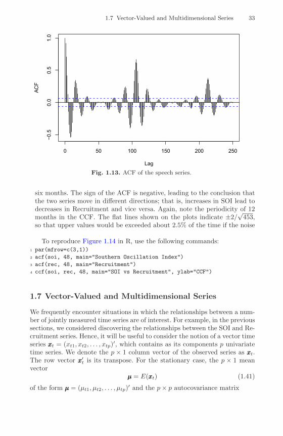
1.7 Vector-Valued and Multidimensional Series 33
0 50 100 150 200 250
−0.5
0.0
0.5
1.0
Lag
ACF
Fig. 1.13. ACF of the speech series.
six months. The sign of the ACF is negative, leading to the conclusion thatthe two series move in different directions; that is, increases in SOI lead todecreases in Recruitment and vice versa. Again, note the periodicity of 12months in the CCF. The flat lines shown on the plots indicate ±2/
√453,
so that upper values would be exceeded about 2.5% of the time if the noisewere white [see (1.36) and (1.39)].
To reproduce Figure 1.14 in R, use the following commands:1 par(mfrow=c(3,1))
2 acf(soi, 48, main="Southern Oscillation Index")
3 acf(rec, 48, main="Recruitment")
4 ccf(soi, rec, 48, main="SOI vs Recruitment", ylab="CCF")
1.7 Vector-Valued and Multidimensional Series
We frequently encounter situations in which the relationships between a num-ber of jointly measured time series are of interest. For example, in the previoussections, we considered discovering the relationships between the SOI and Re-cruitment series. Hence, it will be useful to consider the notion of a vector timeseries xxxt = (xt1, xt2, . . . , xtp)
′, which contains as its components p univariatetime series. We denote the p × 1 column vector of the observed series as xxxt.The row vector xxx′t is its transpose. For the stationary case, the p × 1 meanvector
µµµ = E(xxxt) (1.41)
of the form µµµ = (µt1, µt2, . . . , µtp)′ and the p× p autocovariance matrix
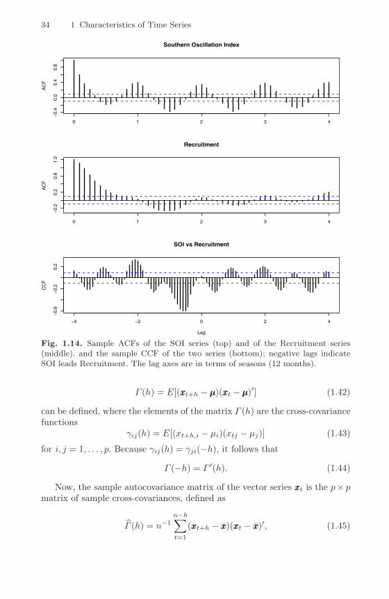
34 1 Characteristics of Time Series
0 1 2 3 4
−0.4
0.0
0.4
0.8
AC
FSouthern Oscillation Index
0 1 2 3 4
−0.2
0.2
0.6
1.0
AC
F
Recruitment
−4 −2 0 2 4
−0.6
−0.2
0.2
Lag
CC
F
SOI vs Recruitment
Fig. 1.14. Sample ACFs of the SOI series (top) and of the Recruitment series(middle), and the sample CCF of the two series (bottom); negative lags indicateSOI leads Recruitment. The lag axes are in terms of seasons (12 months).
Γ (h) = E[(xxxt+h − µµµ)(xxxt − µµµ)′] (1.42)
can be defined, where the elements of the matrix Γ (h) are the cross-covariancefunctions
γij(h) = E[(xt+h,i − µi)(xtj − µj)] (1.43)
for i, j = 1, . . . , p. Because γij(h) = γji(−h), it follows that
Γ (−h) = Γ ′(h). (1.44)
Now, the sample autocovariance matrix of the vector series xxxt is the p× pmatrix of sample cross-covariances, defined as
Γ (h) = n−1n−h∑t=1
(xxxt+h − xxx)(xxxt − xxx)′, (1.45)

1.7 Vector-Valued and Multidimensional Series 35
rows
20
40
60
cols
10
20
30
temperature
4
6
8
10
Fig. 1.15. Two-dimensional time series of temperature measurements taken on arectangular field (64× 36 with 17-foot spacing). Data are from Bazza et al. (1988).
where
xxx = n−1n∑t=1
xxxt (1.46)
denotes the p×1 sample mean vector. The symmetry property of the theoret-ical autocovariance (1.44) extends to the sample autocovariance (1.45), whichis defined for negative values by taking
Γ (−h) = Γ (h)′. (1.47)
In many applied problems, an observed series may be indexed by morethan time alone. For example, the position in space of an experimental unitmight be described by two coordinates, say, s1 and s2. We may proceed inthese cases by defining a multidimensional process xsss as a function of the r×1vector sss = (s1, s2, . . . , sr)
′, where si denotes the coordinate of the ith index.
Example 1.26 Soil Surface Temperatures
As an example, the two-dimensional (r = 2) temperature series xs1,s2 inFigure 1.15 is indexed by a row number s1 and a column number s2 that

36 1 Characteristics of Time Series
represent positions on a 64× 36 spatial grid set out on an agricultural field.The value of the temperature measured at row s1 and column s2, is denotedby xsss = xs1,s2. We can note from the two-dimensional plot that a distinctchange occurs in the character of the two-dimensional surface starting atabout row 40, where the oscillations along the row axis become fairly stableand periodic. For example, averaging over the 36 columns, we may computean average value for each s1 as in Figure 1.16. It is clear that the noisepresent in the first part of the two-dimensional series is nicely averaged out,and we see a clear and consistent temperature signal.
To generate Figures 1.15 and 1.16 in R, use the following commands:1 persp(1:64, 1:36, soiltemp, phi=30, theta=30, scale=FALSE, expand=4,
ticktype="detailed", xlab="rows", ylab="cols",
zlab="temperature")
2 plot.ts(rowMeans(soiltemp), xlab="row", ylab="Average Temperature")
The autocovariance function of a stationary multidimensional process, xsss,can be defined as a function of the multidimensional lag vector, say, hhh =(h1, h2, . . . , hr)
′, as
γ(hhh) = E[(xsss+hhh − µ)(xsss − µ)], (1.48)
whereµ = E(xsss) (1.49)
does not depend on the spatial coordinate sss. For the two dimensional tem-perature process, (1.48) becomes
γ(h1, h2) = E[(xs1+h1,s2+h2− µ)(xs1,s2 − µ)], (1.50)
which is a function of lag, both in the row (h1) and column (h2) directions.The multidimensional sample autocovariance function is defined as
γ(hhh) = (S1S2 · · ·Sr)−1∑s1
∑s2
· · ·∑sr
(xsss+hhh − x)(xsss − x), (1.51)
where sss = (s1, s2, . . . , sr)′ and the range of summation for each argument is
1 ≤ si ≤ Si−hi, for i = 1, . . . , r. The mean is computed over the r-dimensionalarray, that is,
x = (S1S2 · · ·Sr)−1∑s1
∑s2
· · ·∑sr
xs1,s2,··· ,sr , (1.52)
where the arguments si are summed over 1 ≤ si ≤ Si. The multidimensionalsample autocorrelation function follows, as usual, by taking the scaled ratio
ρ(hhh) =γ(hhh)
γ(0). (1.53)

1.7 Vector-Valued and Multidimensional Series 37
row
Aver
age
Tem
pera
ture
0 10 20 30 40 50 60
5.5
6.0
6.5
7.0
7.5
Fig. 1.16. Row averages of the two-dimensional soil temperature profile. xs1 =∑s2xs1,s2/36.
Example 1.27 Sample ACF of the Soil Temperature Series
The autocorrelation function of the two-dimensional (2d) temperature pro-cess can be written in the form
ρ(h1, h2) =γ(h1, h2)
γ(0, 0),
where
γ(h1, h2) = (S1S2)−1∑s1
∑s2
(xs1+h1,s2+h2− x)(xs1,s2 − x)
Figure 1.17 shows the autocorrelation function for the temperature data,and we note the systematic periodic variation that appears along the rows.The autocovariance over columns seems to be strongest for h1 = 0, implyingcolumns may form replicates of some underlying process that has a period-icity over the rows. This idea can be investigated by examining the meanseries over columns as shown in Figure 1.16.
The easiest way (that we know of) to calculate a 2d ACF in R is byusing the fast Fourier transform (FFT) as shown below. Unfortunately, thematerial needed to understand this approach is given in Chapter 4, §4.4. The2d autocovariance function is obtained in two steps and is contained in cs
below; γ(0, 0) is the (1,1) element so that ρ(h1, h2) is obtained by dividingeach element by that value. The 2d ACF is contained in rs below, and therest of the code is simply to arrange the results to yield a nice display.

38 1 Characteristics of Time Series
row lags
−40
−20
0
20
40
colu
mn
lags
−20
−10
0
10
20
AC
F
0.0
0.2
0.4
0.6
0.8
1.0
Fig. 1.17. Two-dimensional autocorrelation function for the soil temperature data.
1 fs = abs(fft(soiltemp-mean(soiltemp)))^2/(64*36)
2 cs = Re(fft(fs, inverse=TRUE)/sqrt(64*36)) # ACovF
3 rs = cs/cs[1,1] # ACF
4 rs2 = cbind(rs[1:41,21:2], rs[1:41,1:21])
5 rs3 = rbind(rs2[41:2,], rs2)
6 par(mar = c(1,2.5,0,0)+.1)
7 persp(-40:40, -20:20, rs3, phi=30, theta=30, expand=30,
scale="FALSE", ticktype="detailed", xlab="row lags",
ylab="column lags", zlab="ACF")
The sampling requirements for multidimensional processes are rather se-vere because values must be available over some uniform grid in order tocompute the ACF. In some areas of application, such as in soil science, wemay prefer to sample a limited number of rows or transects and hope theseare essentially replicates of the basic underlying phenomenon of interest. One-dimensional methods can then be applied. When observations are irregular intime space, modifications to the estimators need to be made. Systematic ap-proaches to the problems introduced by irregularly spaced observations havebeen developed by Journel and Huijbregts (1978) or Cressie (1993). We shallnot pursue such methods in detail here, but it is worth noting that the intro-duction of the variogram
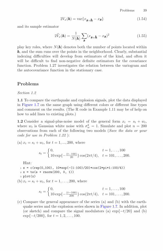
Problems 39
2Vx(hhh) = var{xsss+hhh − xsss} (1.54)
and its sample estimator
2Vx(hhh) =1
N(hhh)
∑sss
(xsss+hhh − xsss)2 (1.55)
play key roles, where N(hhh) denotes both the number of points located withinhhh, and the sum runs over the points in the neighborhood. Clearly, substantialindexing difficulties will develop from estimators of the kind, and often itwill be difficult to find non-negative definite estimators for the covariancefunction. Problem 1.27 investigates the relation between the variogram andthe autocovariance function in the stationary case.
Problems
Section 1.2
1.1 To compare the earthquake and explosion signals, plot the data displayedin Figure 1.7 on the same graph using different colors or different line typesand comment on the results. (The R code in Example 1.11 may be of help onhow to add lines to existing plots.)
1.2 Consider a signal-plus-noise model of the general form xt = st + wt,where wt is Gaussian white noise with σ2
w = 1. Simulate and plot n = 200observations from each of the following two models (Save the data or yourcode for use in Problem 1.22 ):
(a) xt = st + wt, for t = 1, ..., 200, where
st =
{0, t = 1, . . . , 100
10 exp{− (t−100)20 } cos(2πt/4), t = 101, . . . , 200.
Hint:1 s = c(rep(0,100), 10*exp(-(1:100)/20)*cos(2*pi*1:100/4))
2 x = ts(s + rnorm(200, 0, 1))
3 plot(x)
(b)xt = st + wt, for t = 1, . . . , 200, where
st =
{0, t = 1, . . . , 100
10 exp{− (t−100)200 } cos(2πt/4), t = 101, . . . , 200.
(c) Compare the general appearance of the series (a) and (b) with the earth-quake series and the explosion series shown in Figure 1.7. In addition, plot(or sketch) and compare the signal modulators (a) exp{−t/20} and (b)exp{−t/200}, for t = 1, 2, . . . , 100.
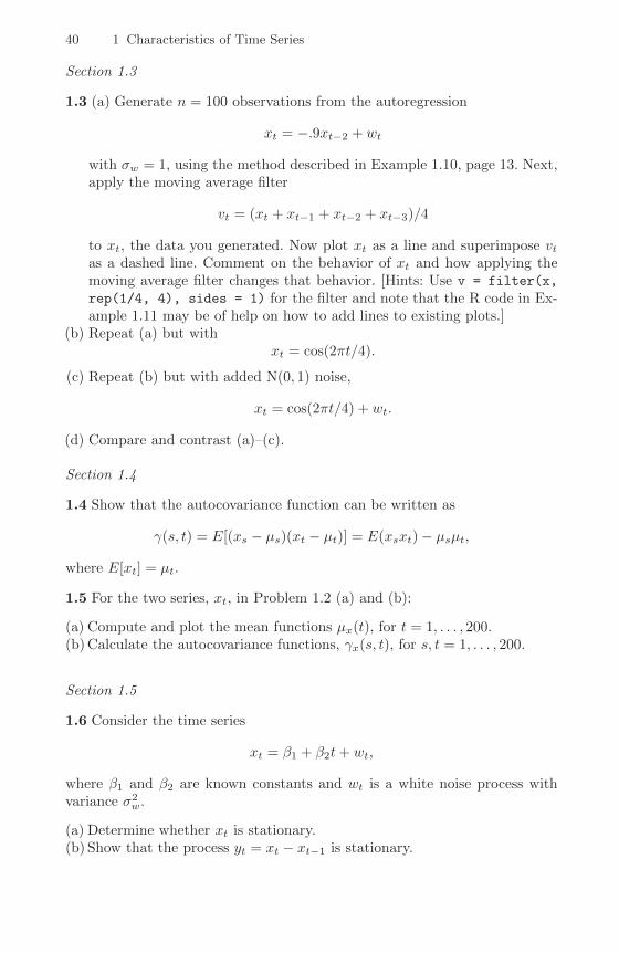
40 1 Characteristics of Time Series
Section 1.3
1.3 (a) Generate n = 100 observations from the autoregression
xt = −.9xt−2 + wt
with σw = 1, using the method described in Example 1.10, page 13. Next,apply the moving average filter
vt = (xt + xt−1 + xt−2 + xt−3)/4
to xt, the data you generated. Now plot xt as a line and superimpose vtas a dashed line. Comment on the behavior of xt and how applying themoving average filter changes that behavior. [Hints: Use v = filter(x,
rep(1/4, 4), sides = 1) for the filter and note that the R code in Ex-ample 1.11 may be of help on how to add lines to existing plots.]
(b) Repeat (a) but withxt = cos(2πt/4).
(c) Repeat (b) but with added N(0, 1) noise,
xt = cos(2πt/4) + wt.
(d) Compare and contrast (a)–(c).
Section 1.4
1.4 Show that the autocovariance function can be written as
γ(s, t) = E[(xs − µs)(xt − µt)] = E(xsxt)− µsµt,
where E[xt] = µt.
1.5 For the two series, xt, in Problem 1.2 (a) and (b):
(a) Compute and plot the mean functions µx(t), for t = 1, . . . , 200.(b) Calculate the autocovariance functions, γx(s, t), for s, t = 1, . . . , 200.
Section 1.5
1.6 Consider the time series
xt = β1 + β2t+ wt,
where β1 and β2 are known constants and wt is a white noise process withvariance σ2
w.
(a) Determine whether xt is stationary.(b) Show that the process yt = xt − xt−1 is stationary.
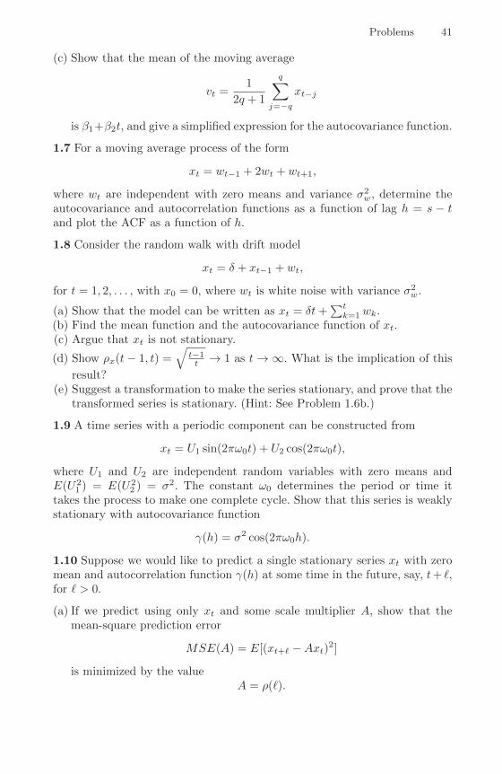
Problems 41
(c) Show that the mean of the moving average
vt =1
2q + 1
q∑j=−q
xt−j
is β1+β2t, and give a simplified expression for the autocovariance function.
1.7 For a moving average process of the form
xt = wt−1 + 2wt + wt+1,
where wt are independent with zero means and variance σ2w, determine the
autocovariance and autocorrelation functions as a function of lag h = s − tand plot the ACF as a function of h.
1.8 Consider the random walk with drift model
xt = δ + xt−1 + wt,
for t = 1, 2, . . . , with x0 = 0, where wt is white noise with variance σ2w.
(a) Show that the model can be written as xt = δt+∑tk=1 wk.
(b) Find the mean function and the autocovariance function of xt.(c) Argue that xt is not stationary.
(d) Show ρx(t− 1, t) =√
t−1t → 1 as t→∞. What is the implication of this
result?(e) Suggest a transformation to make the series stationary, and prove that the
transformed series is stationary. (Hint: See Problem 1.6b.)
1.9 A time series with a periodic component can be constructed from
xt = U1 sin(2πω0t) + U2 cos(2πω0t),
where U1 and U2 are independent random variables with zero means andE(U2
1 ) = E(U22 ) = σ2. The constant ω0 determines the period or time it
takes the process to make one complete cycle. Show that this series is weaklystationary with autocovariance function
γ(h) = σ2 cos(2πω0h).
1.10 Suppose we would like to predict a single stationary series xt with zeromean and autocorrelation function γ(h) at some time in the future, say, t+ `,for ` > 0.
(a) If we predict using only xt and some scale multiplier A, show that themean-square prediction error
MSE(A) = E[(xt+` −Axt)2]
is minimized by the valueA = ρ(`).

42 1 Characteristics of Time Series
(b) Show that the minimum mean-square prediction error is
MSE(A) = γ(0)[1− ρ2(`)].
(c) Show that if xt+` = Axt, then ρ(`) = 1 if A > 0, and ρ(`) = −1 if A < 0.
1.11 Consider the linear process defined in (1.29).
(a) Verify that the autocovariance function of the process is given by (1.30).Use the result to verify your answer to Problem 1.7.
(b) Show that xt exists as a limit in mean square (see Appendix A).
1.12 For two weakly stationary series xt and yt, verify (1.28).
1.13 Consider the two seriesxt = wt
yt = wt − θwt−1 + ut,
where wt and ut are independent white noise series with variances σ2w and σ2
u,respectively, and θ is an unspecified constant.
(a) Express the ACF, ρy(h), for h = 0,±1,±2, . . . of the series yt as a functionof σ2
w, σ2u, and θ.
(b) Determine the CCF, ρxy(h) relating xt and yt.(c) Show that xt and yt are jointly stationary.
1.14 Let xt be a stationary normal process with mean µx and autocovariancefunction γ(h). Define the nonlinear time series
yt = exp{xt}.
(a) Express the mean function E(yt) in terms of µx and γ(0). The momentgenerating function of a normal random variable x with mean µ and vari-ance σ2 is
Mx(λ) = E[exp{λx}] = exp
{µλ+
1
2σ2λ2
}.
(b) Determine the autocovariance function of yt. The sum of the two normalrandom variables xt+h + xt is still a normal random variable.
1.15 Let wt, for t = 0,±1,±2, . . . be a normal white noise process, and con-sider the series
xt = wtwt−1.
Determine the mean and autocovariance function of xt, and state whether itis stationary.

Problems 43
1.16 Consider the seriesxt = sin(2πUt),
t = 1, 2, . . ., where U has a uniform distribution on the interval (0, 1).
(a) Prove xt is weakly stationary.(b) Prove xt is not strictly stationary. [Hint: consider the joint bivariate cdf
(1.18) at the points t = 1, s = 2 with h = 1, and find values of ct, cs wherestrict stationarity does not hold.]
1.17 Suppose we have the linear process xt generated by
xt = wt − θwt−1,
t = 0, 1, 2, . . ., where {wt} is independent and identically distributed withcharacteristic function φw(·), and θ is a fixed constant. [Replace “characteristicfunction” with “moment generating function” if instructed to do so.]
(a) Express the joint characteristic function of x1, x2, . . . , xn, say,
φx1,x2,...,xn(λ1, λ2, . . . , λn),
in terms of φw(·).(b) Deduce from (a) that xt is strictly stationary.
1.18 Suppose that xt is a linear process of the form (1.29). Prove
∞∑h=−∞
|γ(h)| <∞.
Section 1.6
1.19 Suppose x1, . . . , xn is a sample from the process xt = µ + wt − .8wt−1,where wt ∼ wn(0, σ2
w).
(a) Show that mean function is E(xt) = µ.(b) Use (1.33) to calculate the standard error of x for estimating µ.(c) Compare (b) to the case where xt is white noise and show that (b) is
smaller. Explain the result.
1.20 (a) Simulate a series of n = 500 Gaussian white noise observations as inExample 1.8 and compute the sample ACF, ρ(h), to lag 20. Compare thesample ACF you obtain to the actual ACF, ρ(h). [Recall Example 1.19.]
(b) Repeat part (a) using only n = 50. How does changing n affect the results?
1.21 (a) Simulate a series of n = 500 moving average observations as in Ex-ample 1.9 and compute the sample ACF, ρ(h), to lag 20. Compare thesample ACF you obtain to the actual ACF, ρ(h). [Recall Example 1.20.]
(b) Repeat part (a) using only n = 50. How does changing n affect the results?

44 1 Characteristics of Time Series
1.22 Although the model in Problem 1.2(a) is not stationary (Why?), thesample ACF can be informative. For the data you generated in that problem,calculate and plot the sample ACF, and then comment.
1.23 Simulate a series of n = 500 observations from the signal-plus-noisemodel presented in Example 1.12 with σ2
w = 1. Compute the sample ACF tolag 100 of the data you generated and comment.
1.24 For the time series yt described in Example 1.23, verify the stated resultthat ρy(1) = −.47 and ρy(h) = 0 for h > 1.
1.25 A real-valued function g(t), defined on the integers, is non-negative def-inite if and only if
n∑i=1
n∑j=1
aig(ti − tj)aj ≥ 0
for all positive integers n and for all vectors aaa = (a1, a2, . . . , an)′ and ttt =(t1, t2, . . . , tn)′. For the matrix G = {g(ti− tj); i, j = 1, 2, . . . , n}, this impliesthat aaa′Gaaa ≥ 0 for all vectors aaa. It is called positive definite if we can replace‘≥’ with ‘>’ for all aaa 6= 000, the zero vector.
(a) Prove that γ(h), the autocovariance function of a stationary process, is anon-negative definite function.
(b) Verify that the sample autocovariance γ(h) is a non-negative definite func-tion.
Section 1.7
1.26 Consider a collection of time series x1t, x2t, . . . , xNt that are observingsome common signal µt observed in noise processes e1t, e2t, . . . , eNt, with amodel for the j-th observed series given by
xjt = µt + ejt.
Suppose the noise series have zero means and are uncorrelated for differentj. The common autocovariance functions of all series are given by γe(s, t).Define the sample mean
xt =1
N
N∑j=1
xjt.
(a) Show that E[xt] = µt.(b) Show that E[(xt − µ)2)] = N−1γe(t, t).(c) How can we use the results in estimating the common signal?

Problems 45
1.27 A concept used in geostatistics, see Journel and Huijbregts (1978) orCressie (1993), is that of the variogram, defined for a spatial process xsss,sss = (s1, s2), for s1, s2 = 0,±1,±2, ..., as
Vx(hhh) =1
2E[(xsss+hhh − xsss)2],
where hhh = (h1, h2), for h1, h2 = 0,±1,±2, ... Show that, for a stationaryprocess, the variogram and autocovariance functions can be related through
Vx(hhh) = γ(000)− γ(hhh),
where γ(hhh) is the usual lag hhh covariance function and 000 = (0, 0). Note the easyextension to any spatial dimension.
The following problems require the material given in Appendix A
1.28 Suppose xt = β0 +β1t, where β0 and β1 are constants. Prove as n→∞,ρx(h)→ 1 for fixed h, where ρx(h) is the ACF (1.35).
1.29 (a) Suppose xt is a weakly stationary time series with mean zero andwith absolutely summable autocovariance function, γ(h), such that
∞∑h=−∞
γ(h) = 0.
Prove that√n x
p→ 0, where x is the sample mean (1.32).(b) Give an example of a process that satisfies the conditions of part (a). What
is special about this process?
1.30 Let xt be a linear process of the form (A.43)–(A.44). If we define
γ(h) = n−1n∑t=1
(xt+h − µx)(xt − µx),
show thatn1/2
(γ(h)− γ(h)
)= op(1).
Hint: The Markov Inequality
P{|x| ≥ ε} < E|x|ε
can be helpful for the cross-product terms.
1.31 For a linear process of the form
xt =∞∑j=0
φjwt−j ,

46 1 Characteristics of Time Series
where {wt} satisfies the conditions of Theorem A.7 and |φ| < 1, show that
√n
(ρx(1)− ρx(1))√1− ρ2x(1)
d→ N(0, 1),
and construct a 95% confidence interval for φ when ρx(1) = .64 and n = 100.
1.32 Let {xt; t = 0,±1,±2, . . .} be iid(0, σ2).
(a) For h ≥ 1 and k ≥ 1, show that xtxt+h and xsxs+k are uncorrelated forall s 6= t.
(b) For fixed h ≥ 1, show that the h× 1 vector
σ−2n−1/2n∑t=1
(xtxt+1, . . . , xtxt+h)′d→ (z1, . . . , zh)′
where z1, . . . , zh are iid N(0, 1) random variables. [Note: the sequence{xtxt+h; t = 1, 2, . . .} is h-dependent and white noise (0, σ4). Also, re-call the Cramer-Wold device.]
(c) Show, for each h ≥ 1,
n−1/2
[n∑t=1
xtxt+h −n−h∑t=1
(xt − x)(xt+h − x)
]p→ 0 as n→∞
where x = n−1∑nt=1 xt.
(d) Noting that n−1∑nt=1 x
2tp→ σ2, conclude that
n1/2 [ρ(1), . . . , ρ(h)]′ d→ (z1, . . . , zh)′
where ρ(h) is the sample ACF of the data x1, . . . , xn.
2
Time Series Regression and ExploratoryData Analysis
2.1 Introduction
The linear model and its applications are at least as dominant in the timeseries context as in classical statistics. Regression models are important fortime domain models discussed in Chapters 3, 5, and 6, and in the frequencydomain models considered in Chapters 4 and 7. The primary ideas dependon being able to express a response series, say xt, as a linear combinationof inputs, say zt1, zt2, . . . , ztq. Estimating the coefficients β1, β2, . . . , βq in thelinear combinations by least squares provides a method for modeling xt interms of the inputs.
In the time domain applications of Chapter 3, for example, we will expressxt as a linear combination of previous values xt−1, xt−2, . . . , xt−p, of the cur-rently observed series. The outputs xt may also depend on lagged values ofanother series, say yt−1, yt−2, . . . , yt−q, that have influence. It is easy to seethat forecasting becomes an option when prediction models can be formulatedin this form. Time series smoothing and filtering can be expressed in termsof local regression models. Polynomials and regression splines also provideimportant techniques for smoothing.
If one admits sines and cosines as inputs, the frequency domain ideas thatlead to the periodogram and spectrum of Chapter 4 follow from a regressionmodel. Extensions to filters of infinite extent can be handled using regressionin the frequency domain. In particular, many regression problems in the fre-quency domain can be carried out as a function of the periodic componentsof the input and output series, providing useful scientific intuition into fieldslike acoustics, oceanographics, engineering, biomedicine, and geophysics.
The above considerations motivate us to include a separate chapter onregression and some of its applications that is written on an elementary leveland is formulated in terms of time series. The assumption of linearity, sta-tionarity, and homogeneity of variances over time is critical in the regression
© Springer Science+Business Media, LLC 2011
R.H. Shumway and D.S. Stoffer, Time Series Analysis and Its Applications: With R Examples,Springer Texts in Statistics, DOI 10.1007/978-1-4419-7865-3_2,
47

48 2 Time Series Regression and Exploratory Data Analysis
context, and therefore we include some material on transformations and othertechniques useful in exploratory data analysis.
2.2 Classical Regression in the Time Series Context
We begin our discussion of linear regression in the time series context byassuming some output or dependent time series, say, xt, for t = 1, . . . , n,is being influenced by a collection of possible inputs or independent series,say, zt1, zt2, . . . , ztq, where we first regard the inputs as fixed and known.This assumption, necessary for applying conventional linear regression, willbe relaxed later on. We express this relation through the linear regressionmodel
xt = β1zt1 + β2zt2 + · · ·+ βqztq + wt, (2.1)
where β1, β2, . . . , βq are unknown fixed regression coefficients, and {wt} isa random error or noise process consisting of independent and identicallydistributed (iid) normal variables with mean zero and variance σ2
w; we willrelax the iid assumption later. A more general setting within which to embedmean square estimation and linear regression is given in Appendix B, wherewe introduce Hilbert spaces and the Projection Theorem.
Example 2.1 Estimating a Linear Trend
Consider the global temperature data, say xt, shown in Figures 1.2 and 2.1.As discussed in Example 1.2, there is an apparent upward trend in the seriesthat has been used to argue the global warming hypothesis. We might usesimple linear regression to estimate that trend by fitting the model
xt = β1 + β2t+ wt, t = 1880, 1857, . . . , 2009.
This is in the form of the regression model (2.1) when we make the identifi-cation q = 2, zt1 = 1 and zt2 = t. Note that we are making the assumptionthat the errors, wt, are an iid normal sequence, which may not be true.We will address this problem further in §2.3; the problem of autocorrelatederrors is discussed in detail in §5.5. Also note that we could have used, forexample, t = 1, . . . , 130, without affecting the interpretation of the slopecoefficient, β2; only the intercept, β1, would be affected.
Using simple linear regression, we obtained the estimated coefficients β1 =−11.2, and β2 = .006 (with a standard error of .0003) yielding a highlysignificant estimated increase of .6 degrees centigrade per 100 years. Wediscuss the precise way in which the solution was accomplished after theexample. Finally, Figure 2.1 shows the global temperature data, say xt, withthe estimated trend, say xt = −11.2 + .006t, superimposed. It is apparentthat the estimated trend line obtained via simple linear regression does notquite capture the trend of the data and better models will be needed.
To perform this analysis in R, use the following commands:

2.2 Classical Regression in the Time Series Context 49
Fig. 2.1. Global temperature deviations shown in Figure 1.2 with fitted linear trendline.
1 summary(fit <- lm(gtemp~time(gtemp))) # regress gtemp on time
2 plot(gtemp, type="o", ylab="Global Temperature Deviation")
3 abline(fit) # add regression line to the plot
The linear model described by (2.1) above can be conveniently written ina more general notation by defining the column vectors zzzt = (zt1, zt2, . . . , ztq)
′
and βββ = (β1, β2, . . . , βq)′, where ′ denotes transpose, so (2.1) can be written
in the alternate formxt = βββ′zzzt + wt. (2.2)
where wt ∼ iid N(0, σ2w). It is natural to consider estimating the unknown
coefficient vector βββ by minimizing the error sum of squares
Q =
n∑t=1
w2t =
n∑t=1
(xt − βββ′zzzt)2, (2.3)
with respect to β1, β2, . . . , βq. Minimizing Q yields the ordinary least squaresestimator of βββ. This minimization can be accomplished by differentiating (2.3)with respect to the vector βββ or by using the properties of projections. In thenotation above, this procedure gives the normal equations( n∑
t=1
zzztzzz′t
)βββ =
n∑t=1
zzztxt. (2.4)
The notation can be simplified by defining Z = [zzz1 | zzz2 | · · · | zzzn]′ as then × q matrix composed of the n samples of the input variables, the ob-served n × 1 vector xxx = (x1, x2, . . . , xn)′ and the n × 1 vector of errors

50 2 Time Series Regression and Exploratory Data Analysis
www = (w1, w2, . . . , wn)′. In this case, model (2.2) may be written as
xxx = Zβββ +www. (2.5)
The normal equations, (2.4), can now be written as
(Z ′Z) βββ = Z ′xxx (2.6)
and the solutionβββ = (Z ′Z)−1Z ′xxx (2.7)
when the matrix Z ′Z is nonsingular. The minimized error sum of squares(2.3), denoted SSE, can be written as
SSE =n∑t=1
(xt − βββ′zzzt)
2
= (xxx− Zβββ)′(xxx− Zβββ)
= xxx′xxx− βββ′Z ′xxx
= xxx′xxx− xxx′Z(Z ′Z)−1Z ′xxx,
(2.8)
to give some useful versions for later reference. The ordinary least squaresestimators are unbiased, i.e., E(βββ) = βββ, and have the smallest variance withinthe class of linear unbiased estimators.
If the errors wt are normally distributed, βββ is also the maximum likelihoodestimator for βββ and is normally distributed with
cov(βββ) = σ2w
( n∑t=1
zzztzzz′t
)−1= σ2
w(Z ′Z)−1 = σ2wC, (2.9)
whereC = (Z ′Z)−1 (2.10)
is a convenient notation for later equations. An unbiased estimator for thevariance σ2
w is
s2w = MSE =SSE
n− q, (2.11)
where MSE denotes the mean squared error, which is contrasted with themaximum likelihood estimator σ2
w = SSE/n. Under the normal assumption,s2w is distributed proportionally to a chi-squared random variable with n− qdegrees of freedom, denoted by χ2
n−q, and independently of β. It follows that
tn−q =(βi − βi)sw√cii
(2.12)
has the t-distribution with n − q degrees of freedom; cii denotes the i-thdiagonal element of C, as defined in (2.10).
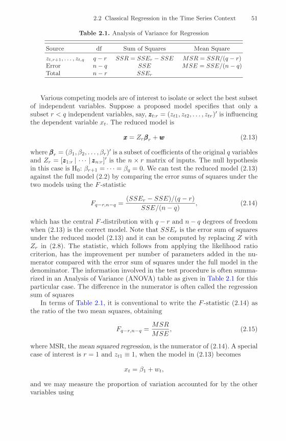
2.2 Classical Regression in the Time Series Context 51
Table 2.1. Analysis of Variance for Regression
Source df Sum of Squares Mean Square
zt,r+1, . . . , zt,q q − r SSR = SSEr − SSE MSR = SSR/(q − r)Error n− q SSE MSE = SSE/(n− q)Total n− r SSEr
Various competing models are of interest to isolate or select the best subsetof independent variables. Suppose a proposed model specifies that only asubset r < q independent variables, say, zzzt:r = (zt1, zt2, . . . , ztr)
′ is influencingthe dependent variable xt. The reduced model is
xxx = Zrβββr +www (2.13)
where βββr = (β1, β2, . . . , βr)′ is a subset of coefficients of the original q variables
and Zr = [zzz1:r | · · · | zzzn:r]′ is the n × r matrix of inputs. The null hypothesisin this case is H0: βr+1 = · · · = βq = 0. We can test the reduced model (2.13)against the full model (2.2) by comparing the error sums of squares under thetwo models using the F -statistic
Fq−r,n−q =(SSEr − SSE)/(q − r)
SSE/(n− q), (2.14)
which has the central F -distribution with q − r and n− q degrees of freedomwhen (2.13) is the correct model. Note that SSEr is the error sum of squaresunder the reduced model (2.13) and it can be computed by replacing Z withZr in (2.8). The statistic, which follows from applying the likelihood ratiocriterion, has the improvement per number of parameters added in the nu-merator compared with the error sum of squares under the full model in thedenominator. The information involved in the test procedure is often summa-rized in an Analysis of Variance (ANOVA) table as given in Table 2.1 for thisparticular case. The difference in the numerator is often called the regressionsum of squares
In terms of Table 2.1, it is conventional to write the F -statistic (2.14) asthe ratio of the two mean squares, obtaining
Fq−r,n−q =MSR
MSE, (2.15)
where MSR, the mean squared regression, is the numerator of (2.14). A specialcase of interest is r = 1 and zt1 ≡ 1, when the model in (2.13) becomes
xt = β1 + wt,
and we may measure the proportion of variation accounted for by the othervariables using
52 2 Time Series Regression and Exploratory Data Analysis
R2 =SSE1 − SSE
SSE1, (2.16)
where the residual sum of squares under the reduced model
SSE1 =n∑t=1
(xt − x)2, (2.17)
in this case is just the sum of squared deviations from the mean x. The mea-sure R2 is also the squared multiple correlation between xt and the variableszt2, zt3, . . . , ztq.
The techniques discussed in the previous paragraph can be used to testvarious models against one another using the F test given in (2.14), (2.15),and the ANOVA table. These tests have been used in the past in a stepwisemanner, where variables are added or deleted when the values from the F -test either exceed or fail to exceed some predetermined levels. The procedure,called stepwise multiple regression, is useful in arriving at a set of usefulvariables. An alternative is to focus on a procedure for model selection thatdoes not proceed sequentially, but simply evaluates each model on its ownmerits. Suppose we consider a normal regression model with k coefficientsand denote the maximum likelihood estimator for the variance as
σ2k =
SSEkn
, (2.18)
where SSEk denotes the residual sum of squares under the model with kregression coefficients. Then, Akaike (1969, 1973, 1974) suggested measuringthe goodness of fit for this particular model by balancing the error of the fitagainst the number of parameters in the model; we define the following.1
Definition 2.1 Akaike’s Information Criterion (AIC)
AIC = log σ2k +
n+ 2k
n, (2.19)
where σ2k is given by (2.18) and k is the number of parameters in the model.
The value of k yielding the minimum AIC specifies the best model. Theidea is roughly that minimizing σ2
k would be a reasonable objective, exceptthat it decreases monotonically as k increases. Therefore, we ought to penalizethe error variance by a term proportional to the number of parameters. Thechoice for the penalty term given by (2.19) is not the only one, and a consid-erable literature is available advocating different penalty terms. A corrected
1 Formally, AIC is defined as −2 logLk + 2k where Lk is the maximized log-likelihood and k is the number of parameters in the model. For the normal regres-sion problem, AIC can be reduced to the form given by (2.19). AIC is an estimateof the Kullback-Leibler discrepency between a true model and a candidate model;see Problems 2.4 and 2.5 for further details.

2.2 Classical Regression in the Time Series Context 53
form, suggested by Sugiura (1978), and expanded by Hurvich and Tsai (1989),can be based on small-sample distributional results for the linear regressionmodel (details are provided in Problems 2.4 and 2.5). The corrected form isdefined as follows.
Definition 2.2 AIC, Bias Corrected (AICc)
AICc = log σ2k +
n+ k
n− k − 2, (2.20)
where σ2k is given by (2.18), k is the number of parameters in the model, and
n is the sample size.
We may also derive a correction term based on Bayesian arguments, as inSchwarz (1978), which leads to the following.
Definition 2.3 Bayesian Information Criterion (BIC)
BIC = log σ2k +
k log n
n, (2.21)
using the same notation as in Definition 2.2.
BIC is also called the Schwarz Information Criterion (SIC); see also Ris-sanen (1978) for an approach yielding the same statistic based on a minimumdescription length argument. Various simulation studies have tended to ver-ify that BIC does well at getting the correct order in large samples, whereasAICc tends to be superior in smaller samples where the relative number ofparameters is large; see McQuarrie and Tsai (1998) for detailed comparisons.In fitting regression models, two measures that have been used in the past areadjusted R-squared, which is essentially s2w, and Mallows Cp, Mallows (1973),which we do not consider in this context.
Example 2.2 Pollution, Temperature and Mortality
The data shown in Figure 2.2 are extracted series from a study by Shumwayet al. (1988) of the possible effects of temperature and pollution on weeklymortality in Los Angeles County. Note the strong seasonal components in allof the series, corresponding to winter-summer variations and the downwardtrend in the cardiovascular mortality over the 10-year period.
A scatterplot matrix, shown in Figure 2.3, indicates a possible linear rela-tion between mortality and the pollutant particulates and a possible relationto temperature. Note the curvilinear shape of the temperature mortalitycurve, indicating that higher temperatures as well as lower temperaturesare associated with increases in cardiovascular mortality.
Based on the scatterplot matrix, we entertain, tentatively, four modelswhere Mt denotes cardiovascular mortality, Tt denotes temperature and Ptdenotes the particulate levels. They are
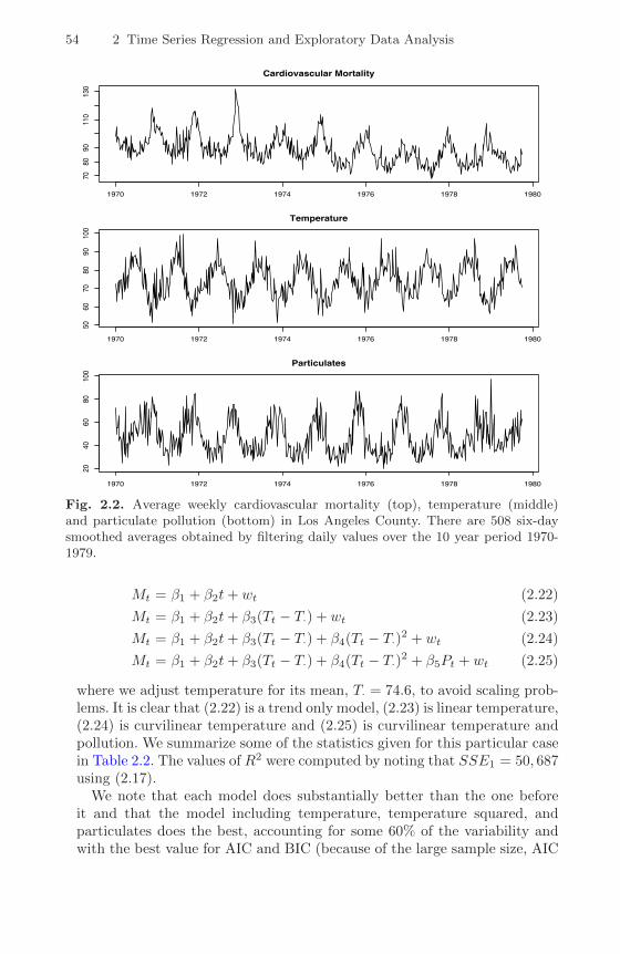
54 2 Time Series Regression and Exploratory Data Analysis
Cardiovascular Mortality
1970 1972 1974 1976 1978 1980
7080
9011
013
0
Temperature
1970 1972 1974 1976 1978 1980
5060
7080
9010
0
Particulates
1970 1972 1974 1976 1978 1980
2040
6080
100
Fig. 2.2. Average weekly cardiovascular mortality (top), temperature (middle)and particulate pollution (bottom) in Los Angeles County. There are 508 six-daysmoothed averages obtained by filtering daily values over the 10 year period 1970-1979.
Mt = β1 + β2t+ wt (2.22)
Mt = β1 + β2t+ β3(Tt − T·) + wt (2.23)
Mt = β1 + β2t+ β3(Tt − T·) + β4(Tt − T·)2 + wt (2.24)
Mt = β1 + β2t+ β3(Tt − T·) + β4(Tt − T·)2 + β5Pt + wt (2.25)
where we adjust temperature for its mean, T· = 74.6, to avoid scaling prob-lems. It is clear that (2.22) is a trend only model, (2.23) is linear temperature,(2.24) is curvilinear temperature and (2.25) is curvilinear temperature andpollution. We summarize some of the statistics given for this particular casein Table 2.2. The values of R2 were computed by noting that SSE1 = 50, 687using (2.17).
We note that each model does substantially better than the one beforeit and that the model including temperature, temperature squared, andparticulates does the best, accounting for some 60% of the variability andwith the best value for AIC and BIC (because of the large sample size, AIC
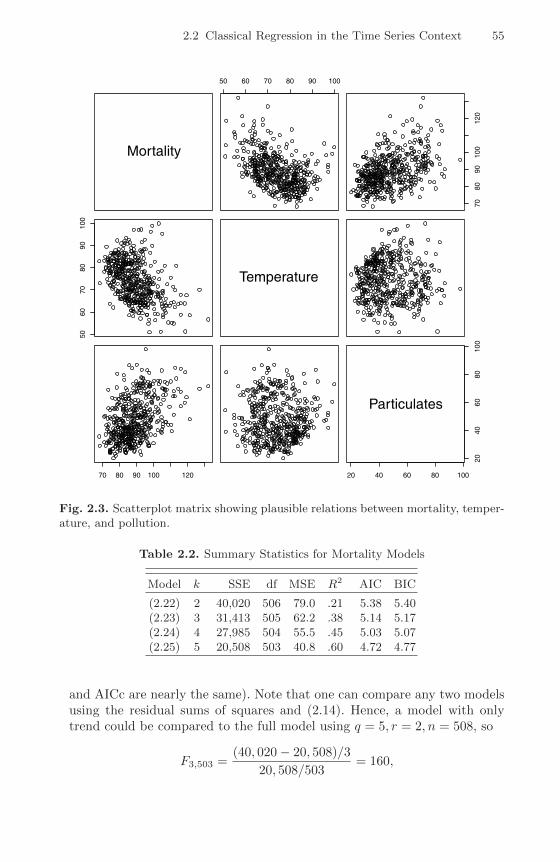
2.2 Classical Regression in the Time Series Context 55
Mortality
50 60 70 80 90 100
7080
9010
012
0
5060
7080
9010
0
Temperature
70 80 90 100 120 20 40 60 80 10020
4060
8010
0
Particulates
Fig. 2.3. Scatterplot matrix showing plausible relations between mortality, temper-ature, and pollution.
Table 2.2. Summary Statistics for Mortality Models
Model k SSE df MSE R2 AIC BIC
(2.22) 2 40,020 506 79.0 .21 5.38 5.40(2.23) 3 31,413 505 62.2 .38 5.14 5.17(2.24) 4 27,985 504 55.5 .45 5.03 5.07(2.25) 5 20,508 503 40.8 .60 4.72 4.77
and AICc are nearly the same). Note that one can compare any two modelsusing the residual sums of squares and (2.14). Hence, a model with onlytrend could be compared to the full model using q = 5, r = 2, n = 508, so
F3,503 =(40, 020− 20, 508)/3
20, 508/503= 160,
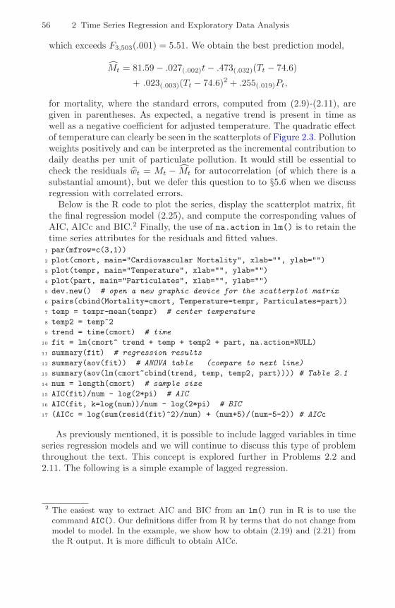
56 2 Time Series Regression and Exploratory Data Analysis
which exceeds F3,503(.001) = 5.51. We obtain the best prediction model,
Mt = 81.59− .027(.002)t− .473(.032)(Tt − 74.6)
+ .023(.003)(Tt − 74.6)2 + .255(.019)Pt,
for mortality, where the standard errors, computed from (2.9)-(2.11), aregiven in parentheses. As expected, a negative trend is present in time aswell as a negative coefficient for adjusted temperature. The quadratic effectof temperature can clearly be seen in the scatterplots of Figure 2.3. Pollutionweights positively and can be interpreted as the incremental contribution todaily deaths per unit of particulate pollution. It would still be essential tocheck the residuals wt = Mt − Mt for autocorrelation (of which there is asubstantial amount), but we defer this question to to §5.6 when we discussregression with correlated errors.
Below is the R code to plot the series, display the scatterplot matrix, fitthe final regression model (2.25), and compute the corresponding values ofAIC, AICc and BIC.2 Finally, the use of na.action in lm() is to retain thetime series attributes for the residuals and fitted values.
1 par(mfrow=c(3,1))
2 plot(cmort, main="Cardiovascular Mortality", xlab="", ylab="")
3 plot(tempr, main="Temperature", xlab="", ylab="")
4 plot(part, main="Particulates", xlab="", ylab="")
5 dev.new() # open a new graphic device for the scatterplot matrix
6 pairs(cbind(Mortality=cmort, Temperature=tempr, Particulates=part))
7 temp = tempr-mean(tempr) # center temperature
8 temp2 = temp^2
9 trend = time(cmort) # time
10 fit = lm(cmort~ trend + temp + temp2 + part, na.action=NULL)
11 summary(fit) # regression results
12 summary(aov(fit)) # ANOVA table (compare to next line)
13 summary(aov(lm(cmort~cbind(trend, temp, temp2, part)))) # Table 2.1
14 num = length(cmort) # sample size
15 AIC(fit)/num - log(2*pi) # AIC
16 AIC(fit, k=log(num))/num - log(2*pi) # BIC
17 (AICc = log(sum(resid(fit)^2)/num) + (num+5)/(num-5-2)) # AICc
As previously mentioned, it is possible to include lagged variables in timeseries regression models and we will continue to discuss this type of problemthroughout the text. This concept is explored further in Problems 2.2 and2.11. The following is a simple example of lagged regression.
2 The easiest way to extract AIC and BIC from an lm() run in R is to use thecommand AIC(). Our definitions differ from R by terms that do not change frommodel to model. In the example, we show how to obtain (2.19) and (2.21) fromthe R output. It is more difficult to obtain AICc.
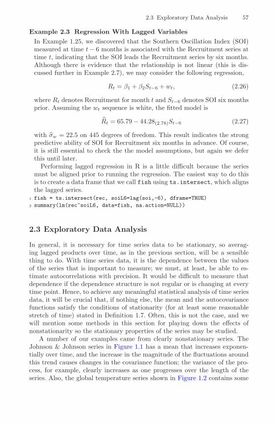
2.3 Exploratory Data Analysis 57
Example 2.3 Regression With Lagged Variables
In Example 1.25, we discovered that the Southern Oscillation Index (SOI)measured at time t− 6 months is associated with the Recruitment series attime t, indicating that the SOI leads the Recruitment series by six months.Although there is evidence that the relationship is not linear (this is dis-cussed further in Example 2.7), we may consider the following regression,
Rt = β1 + β2St−6 + wt, (2.26)
where Rt denotes Recruitment for month t and St−6 denotes SOI six monthsprior. Assuming the wt sequence is white, the fitted model is
Rt = 65.79− 44.28(2.78)St−6 (2.27)
with σw = 22.5 on 445 degrees of freedom. This result indicates the strongpredictive ability of SOI for Recruitment six months in advance. Of course,it is still essential to check the the model assumptions, but again we deferthis until later.
Performing lagged regression in R is a little difficult because the seriesmust be aligned prior to running the regression. The easiest way to do thisis to create a data frame that we call fish using ts.intersect, which alignsthe lagged series.
1 fish = ts.intersect(rec, soiL6=lag(soi,-6), dframe=TRUE)
2 summary(lm(rec~soiL6, data=fish, na.action=NULL))
2.3 Exploratory Data Analysis
In general, it is necessary for time series data to be stationary, so averag-ing lagged products over time, as in the previous section, will be a sensiblething to do. With time series data, it is the dependence between the valuesof the series that is important to measure; we must, at least, be able to es-timate autocorrelations with precision. It would be difficult to measure thatdependence if the dependence structure is not regular or is changing at everytime point. Hence, to achieve any meaningful statistical analysis of time seriesdata, it will be crucial that, if nothing else, the mean and the autocovariancefunctions satisfy the conditions of stationarity (for at least some reasonablestretch of time) stated in Definition 1.7. Often, this is not the case, and wewill mention some methods in this section for playing down the effects ofnonstationarity so the stationary properties of the series may be studied.
A number of our examples came from clearly nonstationary series. TheJohnson & Johnson series in Figure 1.1 has a mean that increases exponen-tially over time, and the increase in the magnitude of the fluctuations aroundthis trend causes changes in the covariance function; the variance of the pro-cess, for example, clearly increases as one progresses over the length of theseries. Also, the global temperature series shown in Figure 1.2 contains some

58 2 Time Series Regression and Exploratory Data Analysis
evidence of a trend over time; human-induced global warming advocates seizeon this as empirical evidence to advance their hypothesis that temperaturesare increasing.
Perhaps the easiest form of nonstationarity to work with is the trend sta-tionary model wherein the process has stationary behavior around a trend.We may write this type of model as
xt = µt + yt (2.28)
where xt are the observations, µt denotes the trend, and yt is a stationaryprocess. Quite often, strong trend, µt, will obscure the behavior of the sta-tionary process, yt, as we shall see in numerous examples. Hence, there is someadvantage to removing the trend as a first step in an exploratory analysis ofsuch time series. The steps involved are to obtain a reasonable estimate of thetrend component, say µt, and then work with the residuals
yt = xt − µt. (2.29)
Consider the following example.
Example 2.4 Detrending Global Temperature
Here we suppose the model is of the form of (2.28),
xt = µt + yt,
where, as we suggested in the analysis of the global temperature data pre-sented in Example 2.1, a straight line might be a reasonable model for thetrend, i.e.,
µt = β1 + β2 t.
In that example, we estimated the trend using ordinary least squares3 andfound
µt = −11.2 + .006 t.
Figure 2.1 shows the data with the estimated trend line superimposed. Toobtain the detrended series we simply subtract µt from the observations, xt,to obtain the detrended series
yt = xt + 11.2− .006 t.
The top graph of Figure 2.4 shows the detrended series. Figure 2.5 showsthe ACF of the original data (top panel) as well as the ACF of the detrendeddata (middle panel).
3 Because the error term, yt, is not assumed to be iid, the reader may feel thatweighted least squares is called for in this case. The problem is, we do not knowthe behavior of yt and that is precisely what we are trying to assess at this stage.A notable result by Grenander and Rosenblatt (1957, Ch 7), however, is thatunder mild conditions on yt, for polynomial regression or periodic regression,asymptotically, ordinary least squares is equivalent to weighted least squares.

2.3 Exploratory Data Analysis 59
Fig. 2.4. Detrended (top) and differenced (bottom) global temperature series. Theoriginal data are shown in Figures 1.2 and 2.1.
To detrend in the series in R, use the following commands. We also showhow to difference and plot the differenced data; we discuss differencing af-ter this example. In addition, we show how to generate the sample ACFsdisplayed in Figure 2.5.
1 fit = lm(gtemp~time(gtemp), na.action=NULL) # regress gtemp on time
2 par(mfrow=c(2,1))
3 plot(resid(fit), type="o", main="detrended")
4 plot(diff(gtemp), type="o", main="first difference")
5 par(mfrow=c(3,1)) # plot ACFs
6 acf(gtemp, 48, main="gtemp")
7 acf(resid(fit), 48, main="detrended")
8 acf(diff(gtemp), 48, main="first difference")
In Example 1.11 and the corresponding Figure 1.10 we saw that a randomwalk might also be a good model for trend. That is, rather than modelingtrend as fixed (as in Example 2.4), we might model trend as a stochasticcomponent using the random walk with drift model,
µt = δ + µt−1 + wt, (2.30)
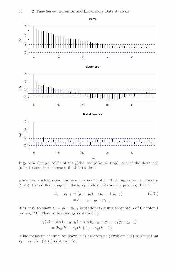
60 2 Time Series Regression and Exploratory Data Analysis
0 10 20 30 40
−0.2
0.2
0.6
1.0
ACF
gtemp
0 10 20 30 40
−0.2
0.2
0.6
1.0
ACF
detrended
0 10 20 30 40
−0.2
0.2
0.6
1.0
Lag
ACF
first difference
Fig. 2.5. Sample ACFs of the global temperature (top), and of the detrended(middle) and the differenced (bottom) series.
where wt is white noise and is independent of yt. If the appropriate model is(2.28), then differencing the data, xt, yields a stationary process; that is,
xt − xt−1 = (µt + yt)− (µt−1 + yt−1) (2.31)
= δ + wt + yt − yt−1.
It is easy to show zt = yt − yt−1 is stationary using footnote 3 of Chapter 1on page 20. That is, because yt is stationary,
γz(h) = cov(zt+h, zt) = cov(yt+h − yt+h−1, yt − yt−1)
= 2γy(h)− γy(h+ 1)− γy(h− 1)
is independent of time; we leave it as an exercise (Problem 2.7) to show thatxt − xt−1 in (2.31) is stationary.

2.3 Exploratory Data Analysis 61
One advantage of differencing over detrending to remove trend is thatno parameters are estimated in the differencing operation. One disadvantage,however, is that differencing does not yield an estimate of the stationaryprocess yt as can be seen in (2.31). If an estimate of yt is essential, thendetrending may be more appropriate. If the goal is to coerce the data tostationarity, then differencing may be more appropriate. Differencing is alsoa viable tool if the trend is fixed, as in Example 2.4. That is, e.g., if µt =β1 + β2 t in the model (2.28), differencing the data produces stationarity (seeProblem 2.6):
xt − xt−1 = (µt + yt)− (µt−1 + yt−1) = β2 + yt − yt−1.
Because differencing plays a central role in time series analysis, it receivesits own notation. The first difference is denoted as
∇xt = xt − xt−1. (2.32)
As we have seen, the first difference eliminates a linear trend. A second differ-ence, that is, the difference of (2.32), can eliminate a quadratic trend, and soon. In order to define higher differences, we need a variation in notation thatwe will use often in our discussion of ARIMA models in Chapter 3.
Definition 2.4 We define the backshift operator by
Bxt = xt−1
and extend it to powers B2xt = B(Bxt) = Bxt−1 = xt−2, and so on. Thus,
Bkxt = xt−k. (2.33)
It is clear that we may then rewrite (2.32) as
∇xt = (1−B)xt, (2.34)
and we may extend the notion further. For example, the second differencebecomes
∇2xt = (1−B)2xt = (1− 2B +B2)xt= xt − 2xt−1 + xt−2
by the linearity of the operator. To check, just take the difference of the firstdifference ∇(∇xt) = ∇(xt − xt−1) = (xt − xt−1)− (xt−1 − xt−2).
Definition 2.5 Differences of order d are defined as
∇d = (1−B)d, (2.35)
where we may expand the operator (1−B)d algebraically to evaluate for higherinteger values of d. When d = 1, we drop it from the notation.
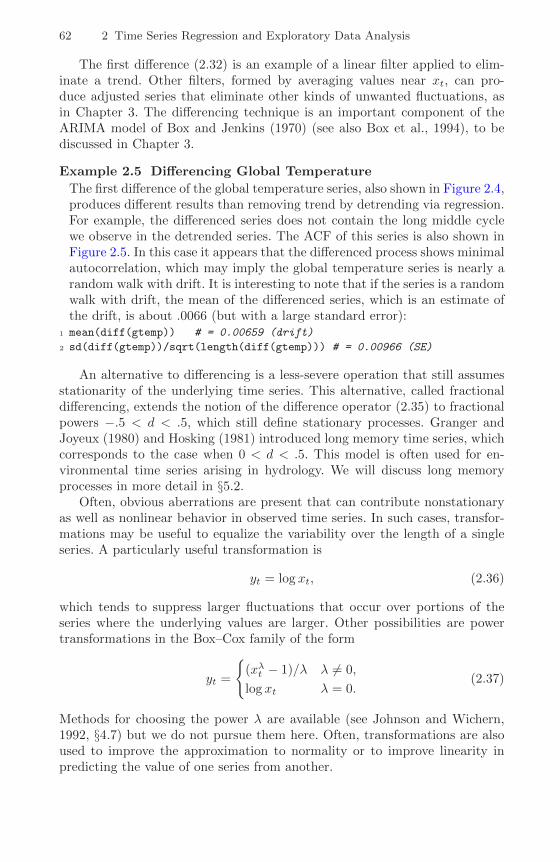
62 2 Time Series Regression and Exploratory Data Analysis
The first difference (2.32) is an example of a linear filter applied to elim-inate a trend. Other filters, formed by averaging values near xt, can pro-duce adjusted series that eliminate other kinds of unwanted fluctuations, asin Chapter 3. The differencing technique is an important component of theARIMA model of Box and Jenkins (1970) (see also Box et al., 1994), to bediscussed in Chapter 3.
Example 2.5 Differencing Global Temperature
The first difference of the global temperature series, also shown in Figure 2.4,produces different results than removing trend by detrending via regression.For example, the differenced series does not contain the long middle cyclewe observe in the detrended series. The ACF of this series is also shown inFigure 2.5. In this case it appears that the differenced process shows minimalautocorrelation, which may imply the global temperature series is nearly arandom walk with drift. It is interesting to note that if the series is a randomwalk with drift, the mean of the differenced series, which is an estimate ofthe drift, is about .0066 (but with a large standard error):
1 mean(diff(gtemp)) # = 0.00659 (drift)
2 sd(diff(gtemp))/sqrt(length(diff(gtemp))) # = 0.00966 (SE)
An alternative to differencing is a less-severe operation that still assumesstationarity of the underlying time series. This alternative, called fractionaldifferencing, extends the notion of the difference operator (2.35) to fractionalpowers −.5 < d < .5, which still define stationary processes. Granger andJoyeux (1980) and Hosking (1981) introduced long memory time series, whichcorresponds to the case when 0 < d < .5. This model is often used for en-vironmental time series arising in hydrology. We will discuss long memoryprocesses in more detail in §5.2.
Often, obvious aberrations are present that can contribute nonstationaryas well as nonlinear behavior in observed time series. In such cases, transfor-mations may be useful to equalize the variability over the length of a singleseries. A particularly useful transformation is
yt = log xt, (2.36)
which tends to suppress larger fluctuations that occur over portions of theseries where the underlying values are larger. Other possibilities are powertransformations in the Box–Cox family of the form
yt =
{(xλt − 1)/λ λ 6= 0,
log xt λ = 0.(2.37)
Methods for choosing the power λ are available (see Johnson and Wichern,1992, §4.7) but we do not pursue them here. Often, transformations are alsoused to improve the approximation to normality or to improve linearity inpredicting the value of one series from another.

2.3 Exploratory Data Analysis 63
varve
0 100 200 300 400 500 600
050
100
150
log(varve)
0 100 200 300 400 500 600
23
45
Fig. 2.6. Glacial varve thicknesses (top) from Massachusetts for n = 634 yearscompared with log transformed thicknesses (bottom).
Example 2.6 Paleoclimatic Glacial Varves
Melting glaciers deposit yearly layers of sand and silt during the springmelting seasons, which can be reconstructed yearly over a period rangingfrom the time deglaciation began in New England (about 12,600 years ago)to the time it ended (about 6,000 years ago). Such sedimentary deposits,called varves, can be used as proxies for paleoclimatic parameters, such astemperature, because, in a warm year, more sand and silt are depositedfrom the receding glacier. Figure 2.6 shows the thicknesses of the yearlyvarves collected from one location in Massachusetts for 634 years, beginning11,834 years ago. For further information, see Shumway and Verosub (1992).Because the variation in thicknesses increases in proportion to the amountdeposited, a logarithmic transformation could remove the nonstationarityobservable in the variance as a function of time. Figure 2.6 shows the originaland transformed varves, and it is clear that this improvement has occurred.We may also plot the histogram of the original and transformed data, asin Problem 2.8, to argue that the approximation to normality is improved.The ordinary first differences (2.34) are also computed in Problem 2.8, andwe note that the first differences have a significant negative correlation at
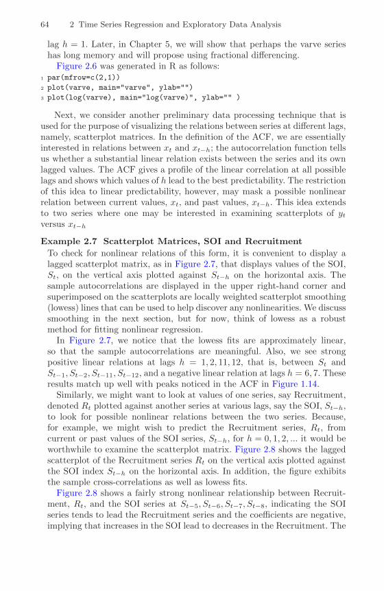
64 2 Time Series Regression and Exploratory Data Analysis
lag h = 1. Later, in Chapter 5, we will show that perhaps the varve serieshas long memory and will propose using fractional differencing.
Figure 2.6 was generated in R as follows:1 par(mfrow=c(2,1))
2 plot(varve, main="varve", ylab="")
3 plot(log(varve), main="log(varve)", ylab="" )
Next, we consider another preliminary data processing technique that isused for the purpose of visualizing the relations between series at different lags,namely, scatterplot matrices. In the definition of the ACF, we are essentiallyinterested in relations between xt and xt−h; the autocorrelation function tellsus whether a substantial linear relation exists between the series and its ownlagged values. The ACF gives a profile of the linear correlation at all possiblelags and shows which values of h lead to the best predictability. The restrictionof this idea to linear predictability, however, may mask a possible nonlinearrelation between current values, xt, and past values, xt−h. This idea extendsto two series where one may be interested in examining scatterplots of ytversus xt−h
Example 2.7 Scatterplot Matrices, SOI and Recruitment
To check for nonlinear relations of this form, it is convenient to display alagged scatterplot matrix, as in Figure 2.7, that displays values of the SOI,St, on the vertical axis plotted against St−h on the horizontal axis. Thesample autocorrelations are displayed in the upper right-hand corner andsuperimposed on the scatterplots are locally weighted scatterplot smoothing(lowess) lines that can be used to help discover any nonlinearities. We discusssmoothing in the next section, but for now, think of lowess as a robustmethod for fitting nonlinear regression.
In Figure 2.7, we notice that the lowess fits are approximately linear,so that the sample autocorrelations are meaningful. Also, we see strongpositive linear relations at lags h = 1, 2, 11, 12, that is, between St andSt−1, St−2, St−11, St−12, and a negative linear relation at lags h = 6, 7. Theseresults match up well with peaks noticed in the ACF in Figure 1.14.
Similarly, we might want to look at values of one series, say Recruitment,denoted Rt plotted against another series at various lags, say the SOI, St−h,to look for possible nonlinear relations between the two series. Because,for example, we might wish to predict the Recruitment series, Rt, fromcurrent or past values of the SOI series, St−h, for h = 0, 1, 2, ... it would beworthwhile to examine the scatterplot matrix. Figure 2.8 shows the laggedscatterplot of the Recruitment series Rt on the vertical axis plotted againstthe SOI index St−h on the horizontal axis. In addition, the figure exhibitsthe sample cross-correlations as well as lowess fits.
Figure 2.8 shows a fairly strong nonlinear relationship between Recruit-ment, Rt, and the SOI series at St−5, St−6, St−7, St−8, indicating the SOIseries tends to lead the Recruitment series and the coefficients are negative,implying that increases in the SOI lead to decreases in the Recruitment. The
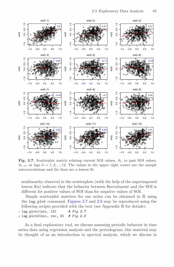
2.3 Exploratory Data Analysis 65
−1.0 −0.5 0.0 0.5 1.0
−1.
00.
00.
51.
0soi(t−1)
soi(t
)
0.6
−1.0 −0.5 0.0 0.5 1.0
−1.
00.
00.
51.
0
soi(t−2)
soi(t
)
0.37
−1.0 −0.5 0.0 0.5 1.0
−1.
00.
00.
51.
0
soi(t−3)
soi(t
)
0.21
−1.0 −0.5 0.0 0.5 1.0
−1.
00.
00.
51.
0
soi(t−4)
soi(t
)
0.05
−1.0 −0.5 0.0 0.5 1.0
−1.
00.
00.
51.
0
soi(t−5)
soi(t
)−0.11
−1.0 −0.5 0.0 0.5 1.0
−1.
00.
00.
51.
0
soi(t−6)
soi(t
)
−0.19
−1.0 −0.5 0.0 0.5 1.0
−1.
00.
00.
51.
0
soi(t−7)
soi(t
)
−0.18
−1.0 −0.5 0.0 0.5 1.0
−1.
00.
00.
51.
0
soi(t−8)
soi(t
)
−0.1
−1.0 −0.5 0.0 0.5 1.0−
1.0
0.0
0.5
1.0
soi(t−9)
soi(t
)
0.05
−1.0 −0.5 0.0 0.5 1.0
−1.
00.
00.
51.
0
soi(t−10)
soi(t
)
0.22
−1.0 −0.5 0.0 0.5 1.0
−1.
00.
00.
51.
0
soi(t−11)
soi(t
)
0.36
−1.0 −0.5 0.0 0.5 1.0
−1.
00.
00.
51.
0
soi(t−12)
soi(t
)
0.41
Fig. 2.7. Scatterplot matrix relating current SOI values, St, to past SOI values,St−h, at lags h = 1, 2, ..., 12. The values in the upper right corner are the sampleautocorrelations and the lines are a lowess fit.
nonlinearity observed in the scatterplots (with the help of the superimposedlowess fits) indicate that the behavior between Recruitment and the SOI isdifferent for positive values of SOI than for negative values of SOI.
Simple scatterplot matrices for one series can be obtained in R usingthe lag.plot command. Figures 2.7 and 2.8 may be reproduced using thefollowing scripts provided with the text (see Appendix R for detials):
1 lag.plot1(soi, 12) # Fig 2.7
2 lag.plot2(soi, rec, 8) # Fig 2.8
As a final exploratory tool, we discuss assessing periodic behavior in timeseries data using regression analysis and the periodogram; this material maybe thought of as an introduction to spectral analysis, which we discuss in
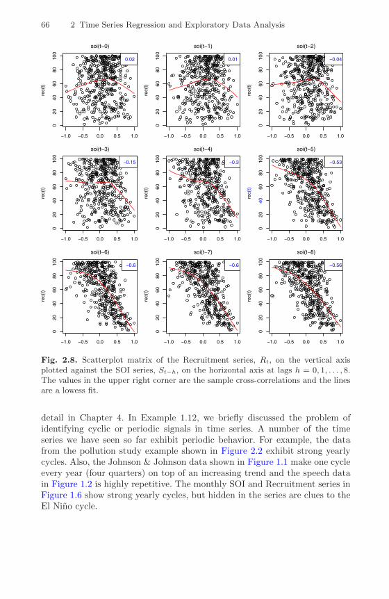
66 2 Time Series Regression and Exploratory Data Analysis
−1.0 −0.5 0.0 0.5 1.0
020
4060
8010
0soi(t−0)
rec(
t)
0.02
−1.0 −0.5 0.0 0.5 1.0
020
4060
8010
0
soi(t−1)
rec(
t)
0.01
−1.0 −0.5 0.0 0.5 1.0
020
4060
8010
0
soi(t−2)
rec(
t)
−0.04
−1.0 −0.5 0.0 0.5 1.0
020
4060
8010
0
soi(t−3)
rec(
t)
−0.15
−1.0 −0.5 0.0 0.5 1.0
020
4060
8010
0soi(t−4)
rec(
t)
−0.3
−1.0 −0.5 0.0 0.5 1.0
020
4060
8010
0
soi(t−5)
rec(
t)
−0.53
−1.0 −0.5 0.0 0.5 1.0
020
4060
8010
0
soi(t−6)
rec(
t)
−0.6
−1.0 −0.5 0.0 0.5 1.0
020
4060
8010
0
soi(t−7)
rec(
t)
−0.6
−1.0 −0.5 0.0 0.5 1.0
020
4060
8010
0soi(t−8)re
c(t)
−0.56
Fig. 2.8. Scatterplot matrix of the Recruitment series, Rt, on the vertical axisplotted against the SOI series, St−h, on the horizontal axis at lags h = 0, 1, . . . , 8.The values in the upper right corner are the sample cross-correlations and the linesare a lowess fit.
detail in Chapter 4. In Example 1.12, we briefly discussed the problem ofidentifying cyclic or periodic signals in time series. A number of the timeseries we have seen so far exhibit periodic behavior. For example, the datafrom the pollution study example shown in Figure 2.2 exhibit strong yearlycycles. Also, the Johnson & Johnson data shown in Figure 1.1 make one cycleevery year (four quarters) on top of an increasing trend and the speech datain Figure 1.2 is highly repetitive. The monthly SOI and Recruitment series inFigure 1.6 show strong yearly cycles, but hidden in the series are clues to theEl Nino cycle.
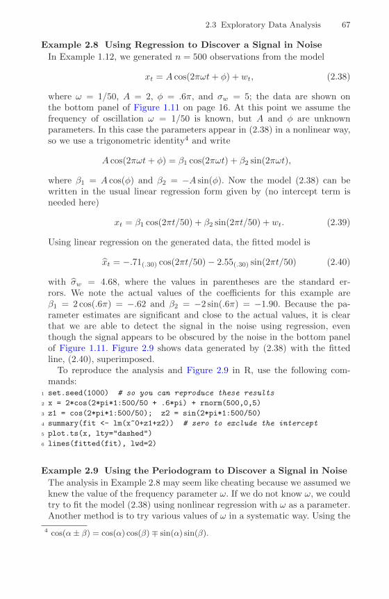
2.3 Exploratory Data Analysis 67
Example 2.8 Using Regression to Discover a Signal in Noise
In Example 1.12, we generated n = 500 observations from the model
xt = A cos(2πωt+ φ) + wt, (2.38)
where ω = 1/50, A = 2, φ = .6π, and σw = 5; the data are shown onthe bottom panel of Figure 1.11 on page 16. At this point we assume thefrequency of oscillation ω = 1/50 is known, but A and φ are unknownparameters. In this case the parameters appear in (2.38) in a nonlinear way,so we use a trigonometric identity4 and write
A cos(2πωt+ φ) = β1 cos(2πωt) + β2 sin(2πωt),
where β1 = A cos(φ) and β2 = −A sin(φ). Now the model (2.38) can bewritten in the usual linear regression form given by (no intercept term isneeded here)
xt = β1 cos(2πt/50) + β2 sin(2πt/50) + wt. (2.39)
Using linear regression on the generated data, the fitted model is
xt = −.71(.30) cos(2πt/50)− 2.55(.30) sin(2πt/50) (2.40)
with σw = 4.68, where the values in parentheses are the standard er-rors. We note the actual values of the coefficients for this example areβ1 = 2 cos(.6π) = −.62 and β2 = −2 sin(.6π) = −1.90. Because the pa-rameter estimates are significant and close to the actual values, it is clearthat we are able to detect the signal in the noise using regression, eventhough the signal appears to be obscured by the noise in the bottom panelof Figure 1.11. Figure 2.9 shows data generated by (2.38) with the fittedline, (2.40), superimposed.
To reproduce the analysis and Figure 2.9 in R, use the following com-mands:
1 set.seed(1000) # so you can reproduce these results
2 x = 2*cos(2*pi*1:500/50 + .6*pi) + rnorm(500,0,5)
3 z1 = cos(2*pi*1:500/50); z2 = sin(2*pi*1:500/50)
4 summary(fit <- lm(x~0+z1+z2)) # zero to exclude the intercept
5 plot.ts(x, lty="dashed")
6 lines(fitted(fit), lwd=2)
Example 2.9 Using the Periodogram to Discover a Signal in Noise
The analysis in Example 2.8 may seem like cheating because we assumed weknew the value of the frequency parameter ω. If we do not know ω, we couldtry to fit the model (2.38) using nonlinear regression with ω as a parameter.Another method is to try various values of ω in a systematic way. Using the
4 cos(α± β) = cos(α) cos(β)∓ sin(α) sin(β).
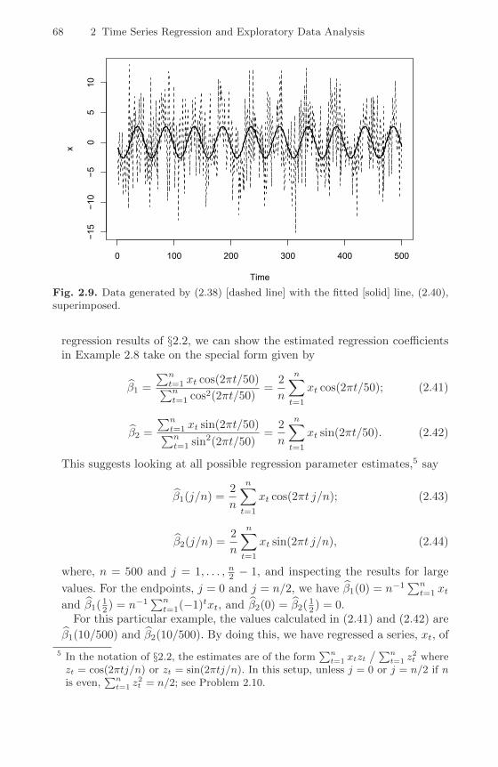
68 2 Time Series Regression and Exploratory Data Analysis
Time
x
0 100 200 300 400 500
−15
−10
−50
510
Fig. 2.9. Data generated by (2.38) [dashed line] with the fitted [solid] line, (2.40),superimposed.
regression results of §2.2, we can show the estimated regression coefficientsin Example 2.8 take on the special form given by
β1 =
∑nt=1 xt cos(2πt/50)∑nt=1 cos2(2πt/50)
=2
n
n∑t=1
xt cos(2πt/50); (2.41)
β2 =
∑nt=1 xt sin(2πt/50)∑nt=1 sin2(2πt/50)
=2
n
n∑t=1
xt sin(2πt/50). (2.42)
This suggests looking at all possible regression parameter estimates,5 say
β1(j/n) =2
n
n∑t=1
xt cos(2πt j/n); (2.43)
β2(j/n) =2
n
n∑t=1
xt sin(2πt j/n), (2.44)
where, n = 500 and j = 1, . . . , n2 − 1, and inspecting the results for large
values. For the endpoints, j = 0 and j = n/2, we have β1(0) = n−1∑nt=1 xt
and β1( 12 ) = n−1
∑nt=1(−1)txt, and β2(0) = β2( 1
2 ) = 0.For this particular example, the values calculated in (2.41) and (2.42) are
β1(10/500) and β2(10/500). By doing this, we have regressed a series, xt, of
5 In the notation of §2.2, the estimates are of the form∑nt=1 xtzt
/ ∑nt=1 z
2t where
zt = cos(2πtj/n) or zt = sin(2πtj/n). In this setup, unless j = 0 or j = n/2 if nis even,
∑nt=1 z
2t = n/2; see Problem 2.10.

2.3 Exploratory Data Analysis 69
0.0 0.1 0.2 0.3 0.4 0.5
01
23
45
67
Frequency
Sca
led
Perio
dogr
am
Fig. 2.10. The scaled periodogram, (2.45), of the 500 observations generated by(2.38); the data are displayed in Figures 1.11 and 2.9.
length n using n regression parameters, so that we will have a perfect fit.The point, however, is that if the data contain any cyclic behavior we arelikely to catch it by performing these saturated regressions.
Next, note that the regression coefficients β1(j/n) and β2(j/n), for eachj, are essentially measuring the correlation of the data with a sinusoid os-cillating at j cycles in n time points.6 Hence, an appropriate measure of thepresence of a frequency of oscillation of j cycles in n time points in the datawould be
P (j/n) = β21(j/n) + β2
2(j/n), (2.45)
which is basically a measure of squared correlation. The quantity (2.45)is sometimes called the periodogram, but we will call P (j/n) the scaledperiodogram and we will investigate its properties in Chapter 4. Figure 2.10shows the scaled periodogram for the data generated by (2.38), and it easilydiscovers the periodic component with frequency ω = .02 = 10/500 eventhough it is difficult to visually notice that component in Figure 1.11 dueto the noise.
Finally, we mention that it is not necessary to run a large regression
xt =
n/2∑j=0
β1(j/n) cos(2πtj/n) + β2(j/n) sin(2πtj/n) (2.46)
to obtain the values of β1(j/n) and β2(j/n) [with β2(0) = β2(1/2) = 0]because they can be computed quickly if n (assumed even here) is a highly
6 Sample correlations are of the form∑t xtzt
/ (∑t x
2t
∑t z
2t
)1/2.
70 2 Time Series Regression and Exploratory Data Analysis
composite integer. There is no error in (2.46) because there are n obser-vations and n parameters; the regression fit will be perfect. The discreteFourier transform (DFT) is a complex-valued weighted average of the datagiven by
d(j/n) = n−1/2n∑t=1
xt exp(−2πitj/n)
= n−1/2
(n∑t=1
xt cos(2πtj/n)− in∑t=1
xt sin(2πtj/n)
) (2.47)
where the frequencies j/n are called the Fourier or fundamental frequencies.Because of a large number of redundancies in the calculation, (2.47) may becomputed quickly using the fast Fourier transform (FFT)7, which is availablein many computing packages such as Matlab R©, S-PLUS R© and R. Note that8
|d(j/n)|2 =1
n
(n∑t=1
xt cos(2πtj/n)
)2
+1
n
(n∑t=1
xt sin(2πtj/n)
)2
(2.48)
and it is this quantity that is called the periodogram; we will write
I(j/n) = |d(j/n)|2.
We may calculate the scaled periodogram, (2.45), using the periodogram as
P (j/n) =4
nI(j/n). (2.49)
We will discuss this approach in more detail and provide examples with datain Chapter 4.
Figure 2.10 can be created in R using the following commands (and thedata already generated in x):
1 I = abs(fft(x))^2/500 # the periodogram
2 P = (4/500)*I[1:250] # the scaled periodogram
3 f = 0:249/500 # frequencies
4 plot(f, P, type="l", xlab="Frequency", ylab="Scaled Periodogram")
2.4 Smoothing in the Time Series Context
In §1.4, we introduced the concept of smoothing a time series, and in Ex-ample 1.9, we discussed using a moving average to smooth white noise. Thismethod is useful in discovering certain traits in a time series, such as long-term
7 Different packages scale the FFT differently; consult the documentation. R cal-culates (2.47) without scaling by n−1/2.
8 If z = a− ib is complex, then |z|2 = zz = (a− ib)(a+ ib) = a2 + b2.

2.4 Smoothing in the Time Series Context 71
Fig. 2.11. The weekly cardiovascular mortality series discussed in Example 2.2smoothed using a five-week moving average and a 53-week moving average.
trend and seasonal components. In particular, if xt represents the observations,then
mt =k∑
j=−k
ajxt−j , (2.50)
where aj = a−j ≥ 0 and∑kj=−k aj = 1 is a symmetric moving average of the
data.
Example 2.10 Moving Average Smoother
For example, Figure 2.11 shows the weekly mortality series discussed inExample 2.2, a five-point moving average (which is essentially a monthlyaverage with k = 2) that helps bring out the seasonal component and a53-point moving average (which is essentially a yearly average with k = 26)that helps bring out the (negative) trend in cardiovascular mortality. In bothcases, the weights, a−k, . . . , a0, . . . , ak, we used were all the same, and equalto 1/(2k + 1).9
To reproduce Figure 2.11 in R:1 ma5 = filter(cmort, sides=2, rep(1,5)/5)
2 ma53 = filter(cmort, sides=2, rep(1,53)/53)
3 plot(cmort, type="p", ylab="mortality")
4 lines(ma5); lines(ma53)
9 Sometimes, the end weights, a−k and ak are set equal to half the value of theother weights.

72 2 Time Series Regression and Exploratory Data Analysis
Fig. 2.12. The weekly cardiovascular mortality series with a cubic trend and cubictrend plus periodic regression.
Many other techniques are available for smoothing time series data basedon methods from scatterplot smoothers. The general setup for a time plot is
xt = ft + yt, (2.51)
where ft is some smooth function of time, and yt is a stationary process. Wemay think of the moving average smoother mt, given in (2.50), as an estimatorof ft. An obvious choice for ft in (2.51) is polynomial regression
ft = β0 + β1t+ · · ·+ βptp. (2.52)
We have seen the results of a linear fit on the global temperature data inExample 2.1. For periodic data, one might employ periodic regression
ft = α0 + α1 cos(2πω1t) + β1 sin(2πω1t)
+ · · ·+ αp cos(2πωpt) + βp sin(2πωpt), (2.53)
where ω1, . . . , ωp are distinct, specified frequencies. In addition, one mightconsider combining (2.52) and (2.53). These smoothers can be applied usingclassical linear regression.
Example 2.11 Polynomial and Periodic Regression Smoothers
Figure 2.12 shows the weekly mortality series with an estimated (via ordi-nary least squares) cubic smoother
ft = β0 + β1t+ β2t2 + β3t
3

2.4 Smoothing in the Time Series Context 73
superimposed to emphasize the trend, and an estimated (via ordinary leastsquares) cubic smoother plus a periodic regression
ft = β0 + β1t+ β2t2 + β3t
3 + α1 cos(2πt/52) + α2 sin(2πt/52)
superimposed to emphasize trend and seasonality.The R commands for this example are as follows (we note that the sam-
pling rate is 1/52, so that wk below is essentially t/52).1 wk = time(cmort) - mean(time(cmort))
2 wk2 = wk^2; wk3 = wk^3
3 cs = cos(2*pi*wk); sn = sin(2*pi*wk)
4 reg1 = lm(cmort~wk + wk2 + wk3, na.action=NULL)
5 reg2 = lm(cmort~wk + wk2 + wk3 + cs + sn, na.action=NULL)
6 plot(cmort, type="p", ylab="mortality")
7 lines(fitted(reg1)); lines(fitted(reg2))
Modern regression techniques can be used to fit general smoothers to thepairs of points (t, xt) where the estimate of ft is smooth. Many of the tech-niques can easily be applied to time series data using the R or S-PLUS sta-tistical packages; see Venables and Ripley (1994, Chapter 10) for details onapplying these methods in S-PLUS (R is similar). A problem with the tech-niques used in Example 2.11 is that they assume ft is the same function overthe range of time, t; we might say that the technique is global. The movingaverage smoothers in Example 2.10 fit the data better because the techniqueis local; that is, moving average smoothers allow for the possibility that ft isa different function over time. We describe some other local methods in thefollowing examples.
Example 2.12 Kernel Smoothing
Kernel smoothing is a moving average smoother that uses a weight function,or kernel, to average the observations. Figure 2.13 shows kernel smoothingof the mortality series, where ft in (2.51) is estimated by
ft =n∑i=1
wi(t)xi, (2.54)
where
wi(t) = K(t−ib
) / n∑j=1
K(t−jb
). (2.55)
are the weights and K(·) is a kernel function. This estimator, which wasoriginally explored by Parzen (1962) and Rosenblatt (1956b), is often calledthe Nadaraya–Watson estimator (Watson, 1966); typically, the normal ker-nel, K(z) = 1√
2πexp(−z2/2), is used. To implement this in R, use the
ksmooth function. The wider the bandwidth, b, the smoother the result.In Figure 2.13, the values of b for this example were b = 5/52 (roughly

74 2 Time Series Regression and Exploratory Data Analysis
Fig. 2.13. Kernel smoothers of the mortality data.
weighted two to three week averages because b/2 is the inner quartile rangeof the kernel) for the seasonal component, and b = 104/52 = 2 (roughlyweighted yearly averages) for the trend component.
Figure 2.13 can be reproduced in R (or S-PLUS) as follows.1 plot(cmort, type="p", ylab="mortality")
2 lines(ksmooth(time(cmort), cmort, "normal", bandwidth=5/52))
3 lines(ksmooth(time(cmort), cmort, "normal", bandwidth=2))
Example 2.13 Lowess and Nearest Neighbor Regression
Another approach to smoothing a time plot is nearest neighbor regression.The technique is based on k-nearest neighbors linear regression, wherein oneuses the data {xt−k/2, . . . , xt, . . . , xt+k/2} to predict xt using linear regres-
sion; the result is ft. For example, Figure 2.14 shows cardiovascular mor-tality and the nearest neighbor method using the R (or S-PLUS) smoothersupsmu. We used k = n/2 to estimate the trend and k = n/100 to esti-mate the seasonal component. In general, supsmu uses a variable windowfor smoothing (see Friedman, 1984), but it can be used for correlated databy fixing the smoothing window, as was done here.
Lowess is a method of smoothing that is rather complex, but the basic ideais close to nearest neighbor regression. Figure 2.14 shows smoothing of mor-tality using the R or S-PLUS function lowess (see Cleveland, 1979). First,a certain proportion of nearest neighbors to xt are included in a weightingscheme; values closer to xt in time get more weight. Then, a robust weightedregression is used to predict xt and obtain the smoothed estimate of ft. Thelarger the fraction of nearest neighbors included, the smoother the estimate

2.4 Smoothing in the Time Series Context 75
nearest neighborm
orta
lity
1970 1972 1974 1976 1978 1980
7080
9011
013
0
lowess
mor
talit
y
1970 1972 1974 1976 1978 1980
7080
9011
013
0
Fig. 2.14. Nearest neighbor (supsmu) and locally weighted regression (lowess)smoothers of the mortality data.
ft will be. In Figure 2.14, the smoother uses about two-thirds of the datato obtain an estimate of the trend component, and the seasonal componentuses 2% of the data.
Figure 2.14 can be reproduced in R or S-PLUS as follows.1 par(mfrow=c(2,1))
2 plot(cmort, type="p", ylab="mortality", main="nearest neighbor")
3 lines(supsmu(time(cmort), cmort, span=.5))
4 lines(supsmu(time(cmort), cmort, span=.01))
5 plot(cmort, type="p", ylab="mortality", main="lowess")
6 lines(lowess(cmort, f=.02)); lines(lowess(cmort, f=2/3))
Example 2.14 Smoothing Splines
An extension of polynomial regression is to first divide time t = 1, . . . , n,into k intervals, [t0 = 1, t1], [t1 + 1, t2] , . . . , [tk−1 + 1, tk = n]. The valuest0, t1, . . . , tk are called knots. Then, in each interval, one fits a regression ofthe form (2.52); typically, p = 3, and this is called cubic splines.
A related method is smoothing splines, which minimizes a compromisebetween the fit and the degree of smoothness given by
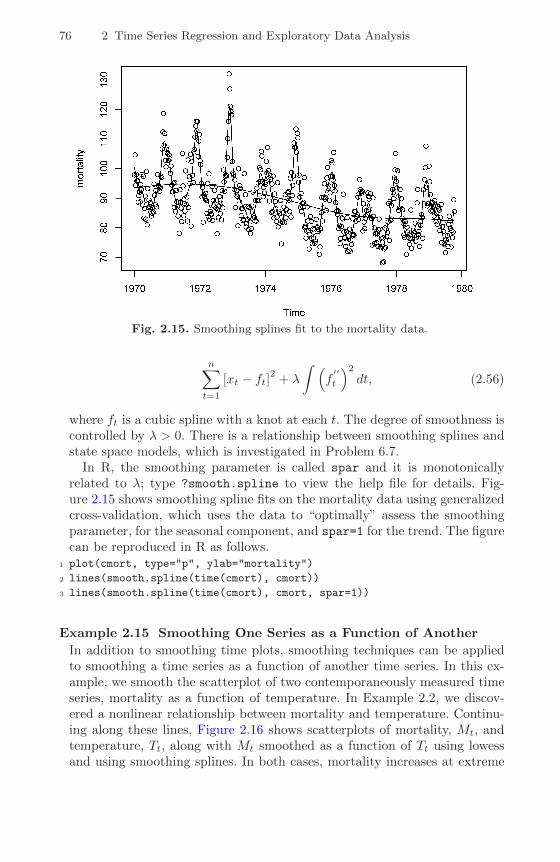
76 2 Time Series Regression and Exploratory Data Analysis
Fig. 2.15. Smoothing splines fit to the mortality data.
n∑t=1
[xt − ft]2 + λ
∫ (f′′
t
)2dt, (2.56)
where ft is a cubic spline with a knot at each t. The degree of smoothness iscontrolled by λ > 0. There is a relationship between smoothing splines andstate space models, which is investigated in Problem 6.7.
In R, the smoothing parameter is called spar and it is monotonicallyrelated to λ; type ?smooth.spline to view the help file for details. Fig-ure 2.15 shows smoothing spline fits on the mortality data using generalizedcross-validation, which uses the data to “optimally” assess the smoothingparameter, for the seasonal component, and spar=1 for the trend. The figurecan be reproduced in R as follows.
1 plot(cmort, type="p", ylab="mortality")
2 lines(smooth.spline(time(cmort), cmort))
3 lines(smooth.spline(time(cmort), cmort, spar=1))
Example 2.15 Smoothing One Series as a Function of Another
In addition to smoothing time plots, smoothing techniques can be appliedto smoothing a time series as a function of another time series. In this ex-ample, we smooth the scatterplot of two contemporaneously measured timeseries, mortality as a function of temperature. In Example 2.2, we discov-ered a nonlinear relationship between mortality and temperature. Continu-ing along these lines, Figure 2.16 shows scatterplots of mortality, Mt, andtemperature, Tt, along with Mt smoothed as a function of Tt using lowessand using smoothing splines. In both cases, mortality increases at extreme

2.4 Smoothing in the Time Series Context 77
50 60 70 80 90 100
7080
9011
013
0
lowess
Temperature
Mor
talit
y
50 60 70 80 90 100
7080
9011
013
0
smoothing splines
Temperature
Mor
talit
y
Fig. 2.16. Smoothers of mortality as a function of temperature using lowess andsmoothing splines.
temperatures, but in an asymmetric way; mortality is higher at colder tem-peratures than at hotter temperatures. The minimum mortality rate seemsto occur at approximately 80◦ F.
Figure 2.16 can be reproduced in R as follows.1 par(mfrow=c(2,1), mar=c(3,2,1,0)+.5, mgp=c(1.6,.6,0))
2 plot(tempr, cmort, main="lowess", xlab="Temperature",
ylab="Mortality")
3 lines(lowess(tempr,cmort))
4 plot(tempr, cmort, main="smoothing splines", xlab="Temperature",
ylab="Mortality")
5 lines(smooth.spline(tempr, cmort))
As a final word of caution, the methods mentioned in this section may nottake into account the fact that the data are serially correlated, and most ofthe techniques have been designed for independent observations. That is, forexample, the smoothers shown in Figure 2.16 are calculated under the falseassumption that the pairs (Mt, Tt), are iid pairs of observations. In addition,

78 2 Time Series Regression and Exploratory Data Analysis
the degree of smoothness used in the previous examples were chosen arbitrarilyto bring out what might be considered obvious features in the data set.
Problems
Section 2.2
2.1 For the Johnson & Johnson data, say yt, shown in Figure 1.1, let xt =log(yt).
(a) Fit the regression model
xt = βt+ α1Q1(t) + α2Q2(t) + α3Q3(t) + α4Q4(t) + wt
where Qi(t) = 1 if time t corresponds to quarter i = 1, 2, 3, 4, and zerootherwise. The Qi(t)’s are called indicator variables. We will assume fornow that wt is a Gaussian white noise sequence. What is the interpreta-tion of the parameters β, α1, α2, α3, and α4? (Detailed code is given inAppendix R on page 574.)
(b) What happens if you include an intercept term in the model in (a)?(c) Graph the data, xt, and superimpose the fitted values, say xt, on the
graph. Examine the residuals, xt− xt, and state your conclusions. Does itappear that the model fits the data well (do the residuals look white)?
2.2 For the mortality data examined in Example 2.2:
(a) Add another component to the regression in (2.25) that accounts for theparticulate count four weeks prior; that is, add Pt−4 to the regression in(2.25). State your conclusion.
(b) Draw a scatterplot matrix of Mt, Tt, Pt and Pt−4 and then calculate thepairwise correlations between the series. Compare the relationship betweenMt and Pt versus Mt and Pt−4.
2.3 Repeat the following exercise six times and then discuss the results. Gen-erate a random walk with drift, (1.4), of length n = 100 with δ = .01 andσw = 1. Call the data xt for t = 1, . . . , 100. Fit the regression xt = βt + wtusing least squares. Plot the data, the mean function (i.e., µt = .01 t) and the
fitted line, xt = β t, on the same graph. Discuss your results.
The following R code may be useful:
1 par(mfcol = c(3,2)) # set up graphics
2 for (i in 1:6){
3 x = ts(cumsum(rnorm(100,.01,1))) # the data
4 reg = lm(x~0+time(x), na.action=NULL) # the regression
5 plot(x) # plot data
6 lines(.01*time(x), col="red", lty="dashed") # plot mean
7 abline(reg, col="blue") } # plot regression line
Problems 79
2.4 Kullback-Leibler Information. Given the random vector yyy, we define theinformation for discriminating between two densities in the same family, in-dexed by a parameter θθθ, say f(yyy; θθθ1) and f(yyy; θθθ2), as
I(θθθ1; θθθ2) =1
nE1 log
f(yyy; θθθ1)
f(yyy; θθθ2), (2.57)
where E1 denotes expectation with respect to the density determined by θθθ1.For the Gaussian regression model, the parameters are θθθ = (βββ′, σ2)′. Showthat we obtain
I(θθθ1; θθθ2) =1
2
(σ21
σ22
− logσ21
σ22
− 1
)+
1
2
(βββ1 − βββ2)′Z ′Z(βββ1 − βββ2)
nσ22
(2.58)
in that case.
2.5 Model Selection. Both selection criteria (2.19) and (2.20) are derived frominformation theoretic arguments, based on the well-known Kullback-Leiblerdiscrimination information numbers (see Kullback and Leibler, 1951, Kull-back, 1958). We give an argument due to Hurvich and Tsai (1989). We thinkof the measure (2.58) as measuring the discrepancy between the two densities,characterized by the parameter values θθθ′1 = (βββ′1, σ
21)′ and θθθ′2 = (βββ′2, σ
22)′. Now,
if the true value of the parameter vector is θθθ1, we argue that the best modelwould be one that minimizes the discrepancy between the theoretical valueand the sample, say I(θθθ1; θθθ). Because θθθ1 will not be known, Hurvich and Tsai
(1989) considered finding an unbiased estimator for E1[I(βββ1, σ21 ; βββ,σ
2)], where
I(βββ1, σ21 ; βββ,σ
2) =1
2
(σ21
σ2− log
σ21
σ2− 1
)+
1
2
(βββ1 − βββ)′Z ′Z(βββ1 − βββ)
nσ2
and βββ is a k × 1 regression vector. Show that
E1[I(βββ1, σ21 ; βββ,σ
2)] =1
2
(− log σ2
1 + E1 log σ2 +n+ k
n− k − 2− 1
), (2.59)
using the distributional properties of the regression coefficients and error vari-ance. An unbiased estimator for E1 log σ2 is log σ2. Hence, we have shownthat the expectation of the above discrimination information is as claimed.As models with differing dimensions k are considered, only the second andthird terms in (2.59) will vary and we only need unbiased estimators for thosetwo terms. This gives the form of AICc quoted in (2.20) in the chapter. Youwill need the two distributional results
nσ2
σ21
∼ χ2n−k and
(βββ − βββ1)′Z ′Z(βββ − βββ1)
σ21
∼ χ2k
The two quantities are distributed independently as chi-squared distributionswith the indicated degrees of freedom. If x ∼ χ2
n, E(1/x) = 1/(n− 2).
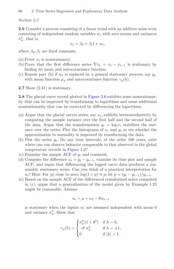
80 2 Time Series Regression and Exploratory Data Analysis
Section 2.3
2.6 Consider a process consisting of a linear trend with an additive noise termconsisting of independent random variables wt with zero means and variancesσ2w, that is,
xt = β0 + β1t+ wt,
where β0, β1 are fixed constants.
(a) Prove xt is nonstationary.(b) Prove that the first difference series ∇xt = xt − xt−1 is stationary by
finding its mean and autocovariance function.(c) Repeat part (b) if wt is replaced by a general stationary process, say yt,
with mean function µy and autocovariance function γy(h).
2.7 Show (2.31) is stationary.
2.8 The glacial varve record plotted in Figure 2.6 exhibits some nonstationar-ity that can be improved by transforming to logarithms and some additionalnonstationarity that can be corrected by differencing the logarithms.
(a) Argue that the glacial varves series, say xt, exhibits heteroscedasticity bycomputing the sample variance over the first half and the second half ofthe data. Argue that the transformation yt = log xt stabilizes the vari-ance over the series. Plot the histograms of xt and yt to see whether theapproximation to normality is improved by transforming the data.
(b) Plot the series yt. Do any time intervals, of the order 100 years, existwhere one can observe behavior comparable to that observed in the globaltemperature records in Figure 1.2?
(c) Examine the sample ACF of yt and comment.(d) Compute the difference ut = yt − yt−1, examine its time plot and sample
ACF, and argue that differencing the logged varve data produces a rea-sonably stationary series. Can you think of a practical interpretation forut? Hint: For |p| close to zero, log(1 + p) ≈ p; let p = (yt − yt−1)/yt−1.
(e) Based on the sample ACF of the differenced transformed series computedin (c), argue that a generalization of the model given by Example 1.23might be reasonable. Assume
ut = µ+ wt − θwt−1
is stationary when the inputs wt are assumed independent with mean 0and variance σ2
w. Show that
γu(h) =
σ2w(1 + θ2) if h = 0,
−θ σ2w if h = ±1,
0 if |h| > 1.

Problems 81
(f) Based on part (e), use ρu(1) and the estimate of the variance of ut, γu(0),to derive estimates of θ and σ2
w. This is an application of the method ofmoments from classical statistics, where estimators of the parameters arederived by equating sample moments to theoretical moments.
2.9 In this problem, we will explore the periodic nature of St, the SOI seriesdisplayed in Figure 1.5.
(a) Detrend the series by fitting a regression of St on time t. Is there a signif-icant trend in the sea surface temperature? Comment.
(b) Calculate the periodogram for the detrended series obtained in part (a).Identify the frequencies of the two main peaks (with an obvious one at thefrequency of one cycle every 12 months). What is the probable El Ninocycle indicated by the minor peak?
2.10 Consider the model (2.46) used in Example 2.9,
xt =n∑j=0
β1(j/n) cos(2πtj/n) + β2(j/n) sin(2πtj/n).
(a) Display the model design matrix Z [see (2.5)] for n = 4.(b) Show numerically that the columns of Z in part (a) satisfy part (d) and
then display (Z ′Z)−1 for this case.(c) If x1, x2, x3, x4 are four observations, write the estimates of the four betas,
β1(0), β1(1/4), β2(1/4), β1(1/2), in terms of the observations.(d) Verify that for any positive integer n and j, k = 0, 1, . . . , [[n/2]], where [[·]]
denotes the greatest integer function:10
(i) Except for j = 0 or j = n/2,
n∑t=1
cos2(2πtj/n) =
n∑t=1
sin2(2πtj/n) = n/2
.(ii) When j = 0 or j = n/2,
n∑t=1
cos2(2πtj/n) = n but
n∑t=1
sin2(2πtj/n) = 0.
(iii) For j 6= k,
n∑t=1
cos(2πtj/n) cos(2πtk/n) =n∑t=1
sin(2πtj/n) sin(2πtk/n) = 0.
Also, for any j and k,
n∑t=1
cos(2πtj/n) sin(2πtk/n) = 0.
10 Some useful facts: 2 cos(α) = eiα + e−iα, 2i sin(α) = eiα − e−iα, and∑nt=1 z
t =z(1− zn)/(1− z) for z 6= 1.

82 2 Time Series Regression and Exploratory Data Analysis
Section 2.4
2.11 Consider the two weekly time series oil and gas. The oil series is indollars per barrel, while the gas series is in cents per gallon; see Appendix Rfor details.
(a) Plot the data on the same graph. Which of the simulated series displayed in§1.3 do these series most resemble? Do you believe the series are stationary(explain your answer)?
(b) In economics, it is often the percentage change in price (termed growth rateor return), rather than the absolute price change, that is important. Arguethat a transformation of the form yt = ∇ log xt might be applied to thedata, where xt is the oil or gas price series [see the hint in Problem 2.8(d)].
(c) Transform the data as described in part (b), plot the data on the samegraph, look at the sample ACFs of the transformed data, and comment.[Hint: poil = diff(log(oil)) and pgas = diff(log(gas)).]
(d) Plot the CCF of the transformed data and comment The small, but signif-icant values when gas leads oil might be considered as feedback. [Hint:ccf(poil, pgas) will have poil leading for negative lag values.]
(e) Exhibit scatterplots of the oil and gas growth rate series for up to threeweeks of lead time of oil prices; include a nonparametric smoother in eachplot and comment on the results (e.g., Are there outliers? Are the rela-tionships linear?). [Hint: lag.plot2(poil, pgas, 3).]
(f) There have been a number of studies questioning whether gasoline pricesrespond more quickly when oil prices are rising than when oil prices arefalling (“asymmetry”). We will attempt to explore this question here withsimple lagged regression; we will ignore some obvious problems such asoutliers and autocorrelated errors, so this will not be a definitive analysis.Let Gt and Ot denote the gas and oil growth rates.
(i) Fit the regression (and comment on the results)
Gt = α1 + α2It + β1Ot + β2Ot−1 + wt,
where It = 1 if Ot ≥ 0 and 0 otherwise (It is the indicator of nogrowth or positive growth in oil price). Hint:
1 indi = ifelse(poil < 0, 0, 1)
2 mess = ts.intersect(pgas, poil, poilL = lag(poil,-1), indi)
3 summary(fit <- lm(pgas~ poil + poilL + indi, data=mess))
(ii) What is the fitted model when there is negative growth in oil price attime t? What is the fitted model when there is no or positive growthin oil price? Do these results support the asymmetry hypothesis?
(iii) Analyze the residuals from the fit and comment.
2.12 Use two different smoothing techniques described in §2.4 to estimate thetrend in the global temperature series displayed in Figure 1.2. Comment.

3
ARIMA Models
3.1 Introduction
In Chapters 1 and 2, we introduced autocorrelation and cross-correlation func-tions (ACFs and CCFs) as tools for clarifying relations that may occur withinand between time series at various lags. In addition, we explained how tobuild linear models based on classical regression theory for exploiting the as-sociations indicated by large values of the ACF or CCF. The time domain, orregression, methods of this chapter are appropriate when we are dealing withpossibly nonstationary, shorter time series; these series are the rule ratherthan the exception in many applications. In addition, if the emphasis is onforecasting future values, then the problem is easily treated as a regressionproblem. This chapter develops a number of regression techniques for time se-ries that are all related to classical ordinary and weighted or correlated leastsquares.
Classical regression is often insufficient for explaining all of the interestingdynamics of a time series. For example, the ACF of the residuals of the sim-
Chapter 2) reveals additional structure in the data that the regression did notcapture. Instead, the introduction of correlation as a phenomenon that maybe generated through lagged linear relations leads to proposing the autore-gressive (AR) and autoregressive moving average (ARMA) models. Addingnonstationary models to the mix leads to the autoregressive integrated mov-ing average (ARIMA) model popularized in the landmark work by Box andJenkins (1970). The Box–Jenkins method for identifying a plausible ARIMAmodel is given in this chapter along with techniques for parameter estimationand forecasting for these models. A partial theoretical justification of the useof ARMA models is discussed in Appendix B, §B.4.
© Springer Science+Business Media, LLC 2011
R.H. Shumway and D.S. Stoffer, Time Series Analysis and Its Applications: With R Examples, 83
ple linear regression fit to the global temperature data (see Example 2.4 of
Springer Texts in Statistics, DOI 10.1007/978-1-4419-7865-3_3,

84 3 ARIMA Models
3.2 Autoregressive Moving Average Models
The classical regression model of Chapter 2 was developed for the static case,namely, we only allow the dependent variable to be influenced by currentvalues of the independent variables. In the time series case, it is desirableto allow the dependent variable to be influenced by the past values of theindependent variables and possibly by its own past values. If the present canbe plausibly modeled in terms of only the past values of the independentinputs, we have the enticing prospect that forecasting will be possible.
Introduction to Autoregressive Models
Autoregressive models are based on the idea that the current value of theseries, xt, can be explained as a function of p past values, xt−1, xt−2, . . . , xt−p,where p determines the number of steps into the past needed to forecastthe current value. As a typical case, recall Example 1.10 in which data weregenerated using the model
xt = xt−1 − .90xt−2 + wt,
where wt is white Gaussian noise with σ2w = 1. We have now assumed the
current value is a particular linear function of past values. The regularity thatpersists in Figure 1.9 gives an indication that forecasting for such a modelmight be a distinct possibility, say, through some version such as
xnn+1 = xn − .90xn−1,
where the quantity on the left-hand side denotes the forecast at the nextperiod n + 1 based on the observed data, x1, x2, . . . , xn. We will make thisnotion more precise in our discussion of forecasting (§3.5).
The extent to which it might be possible to forecast a real data series fromits own past values can be assessed by looking at the autocorrelation functionand the lagged scatterplot matrices discussed in Chapter 2. For example, thelagged scatterplot matrix for the Southern Oscillation Index (SOI), shownin Figure 2.7, gives a distinct indication that lags 1 and 2, for example, arelinearly associated with the current value. The ACF shown in Figure 1.14shows relatively large positive values at lags 1, 2, 12, 24, and 36 and largenegative values at 18, 30, and 42. We note also the possible relation betweenthe SOI and Recruitment series indicated in the scatterplot matrix shown inFigure 2.8. We will indicate in later sections on transfer function and vectorAR modeling how to handle the dependence on values taken by other series.
The preceding discussion motivates the following definition.
Definition 3.1 An autoregressive model of order p, abbreviated AR(p),is of the form
xt = φ1xt−1 + φ2xt−2 + · · ·+ φpxt−p + wt, (3.1)
3.2 Autoregressive Moving Average Models 85
where xt is stationary, and φ1, φ2, . . . , φp are constants (φp 6= 0). Although itis not necessary yet, we assume that wt is a Gaussian white noise series withmean zero and variance σ2
w, unless otherwise stated. The mean of xt in (3.1)is zero. If the mean, µ, of xt is not zero, replace xt by xt − µ in (3.1),
xt − µ = φ1(xt−1 − µ) + φ2(xt−2 − µ) + · · ·+ φp(xt−p − µ) + wt,
or writext = α+ φ1xt−1 + φ2xt−2 + · · ·+ φpxt−p + wt, (3.2)
where α = µ(1− φ1 − · · · − φp).
We note that (3.2) is similar to the regression model of §2.2, and hencethe term auto (or self) regression. Some technical difficulties, however, developfrom applying that model because the regressors, xt−1, . . . , xt−p, are randomcomponents, whereas zzzt was assumed to be fixed. A useful form follows byusing the backshift operator (2.33) to write the AR(p) model, (3.1), as
(1− φ1B − φ2B2 − · · · − φpBp)xt = wt, (3.3)
or even more concisely asφ(B)xt = wt. (3.4)
The properties of φ(B) are important in solving (3.4) for xt. This leads to thefollowing definition.
Definition 3.2 The autoregressive operator is defined to be
φ(B) = 1− φ1B − φ2B2 − · · · − φpBp. (3.5)
We initiate the investigation of AR models by considering the first-ordermodel, AR(1), given by xt = φxt−1 +wt. Iterating backwards k times, we get
xt = φxt−1 + wt = φ(φxt−2 + wt−1) + wt= φ2xt−2 + φwt−1 + wt...
= φkxt−k +
k−1∑j=0
φjwt−j .
This method suggests that, by continuing to iterate backward, and providedthat |φ| < 1 and xt is stationary, we can represent an AR(1) model as a linearprocess given by1
xt =∞∑j=0
φjwt−j . (3.6)
1 Note that limk→∞E(xt −
∑k−1j=0 φ
jwt−j)2
= limk→∞ φ2kE
(x2t−k
)= 0, so (3.6)
exists in the mean square sense (see Appendix A for a definition).

86 3 ARIMA Models
The AR(1) process defined by (3.6) is stationary with mean
E(xt) =
∞∑j=0
φjE(wt−j) = 0,
and autocovariance function,
γ(h) = cov(xt+h, xt) = E
( ∞∑j=0
φjwt+h−j
)( ∞∑k=0
φkwt−k
)= E
[(wt+h + · · ·+ φhwt + φh+1wt−1 + · · ·
)(wt + φwt−1 + · · · )
]= σ2
w
∞∑j=0
φh+jφj = σ2wφ
h∞∑j=0
φ2j =σ2wφ
h
1− φ2, h ≥ 0.
(3.7)
Recall that γ(h) = γ(−h), so we will only exhibit the autocovariance functionfor h ≥ 0. From (3.7), the ACF of an AR(1) is
ρ(h) =γ(h)
γ(0)= φh, h ≥ 0, (3.8)
and ρ(h) satisfies the recursion
ρ(h) = φ ρ(h− 1), h = 1, 2, . . . . (3.9)
We will discuss the ACF of a general AR(p) model in §3.4.
Example 3.1 The Sample Path of an AR(1) Process
Figure 3.1 shows a time plot of two AR(1) processes, one with φ = .9 andone with φ = −.9; in both cases, σ2
w = 1. In the first case, ρ(h) = .9h, forh ≥ 0, so observations close together in time are positively correlated witheach other. This result means that observations at contiguous time pointswill tend to be close in value to each other; this fact shows up in the topof Figure 3.1 as a very smooth sample path for xt. Now, contrast this withthe case in which φ = −.9, so that ρ(h) = (−.9)h, for h ≥ 0. This resultmeans that observations at contiguous time points are negatively correlatedbut observations two time points apart are positively correlated. This factshows up in the bottom of Figure 3.1, where, for example, if an observation,xt, is positive, the next observation, xt+1, is typically negative, and the nextobservation, xt+2, is typically positive. Thus, in this case, the sample pathis very choppy.
The following R code can be used to obtain a figure similar to Figure 3.1:1 par(mfrow=c(2,1))
2 plot(arima.sim(list(order=c(1,0,0), ar=.9), n=100), ylab="x",
main=(expression(AR(1)~~~phi==+.9)))
3 plot(arima.sim(list(order=c(1,0,0), ar=-.9), n=100), ylab="x",
main=(expression(AR(1)~~~phi==-.9)))

3.2 Autoregressive Moving Average Models 87
AR(1) = +.9
0 20 40 60 80 100
−6−4
−20
24
AR(1) = −.9
0 20 40 60 80 100
−6−4
−20
24
6
Fig. 3.1. Simulated AR(1) models: φ = .9 (top); φ = −.9 (bottom).
Example 3.2 Explosive AR Models and Causality
In Example 1.18, it was discovered that the random walk xt = xt−1 + wtis not stationary. We might wonder whether there is a stationary AR(1)process with |φ| > 1. Such processes are called explosive because the valuesof the time series quickly become large in magnitude. Clearly, because |φ|jincreases without bound as j →∞,
∑k−1j=0 φ
jwt−j will not converge (in meansquare) as k →∞, so the intuition used to get (3.6) will not work directly.We can, however, modify that argument to obtain a stationary model asfollows. Write xt+1 = φxt + wt+1, in which case,
xt = φ−1xt+1 − φ−1wt+1 = φ−1(φ−1xt+2 − φ−1wt+2
)− φ−1wt+1
...
= φ−kxt+k −k−1∑j=1
φ−jwt+j , (3.10)
by iterating forward k steps. Because |φ|−1 < 1, this result suggests thestationary future dependent AR(1) model
88 3 ARIMA Models
xt = −∞∑j=1
φ−jwt+j . (3.11)
The reader can verify that this is stationary and of the AR(1) form xt =φxt−1 + wt. Unfortunately, this model is useless because it requires us toknow the future to be able to predict the future. When a process does notdepend on the future, such as the AR(1) when |φ| < 1, we will say the processis causal. In the explosive case of this example, the process is stationary, butit is also future dependent, and not causal.
Example 3.3 Every Explosion Has a Cause
Excluding explosive models from consideration is not a problem because themodels have causal counterparts. For example, if
xt = φxt−1 + wt with |φ| > 1
and wt ∼ iid N(0, σ2w), then using (3.11), {xt} is a non-causal stationary
Gaussian process with E(xt) = 0 and
γx(h) = cov(xt+h, xt) = cov
− ∞∑j=1
φ−jwt+h+j , −∞∑k=1
φ−kwt+k
= σ2
wφ−2 φ−h/(1− φ−2).
Thus, using (3.7), the causal process defined by
yt = φ−1yt−1 + vt
where vt ∼ iid N(0, σ2wφ−2) is stochastically equal to the xt process (i.e.,
all finite distributions of the processes are the same). For example, if xt =2xt−1 +wt with σ2
w = 1, then yt = 12yt−1 +vt with σ2
v = 1/4 is an equivalentcausal process (see Problem 3.3). This concept generalizes to higher orders,but it is easier to show using Chapter 4 techniques; see Example 4.7.
The technique of iterating backward to get an idea of the stationary so-lution of AR models works well when p = 1, but not for larger orders. Ageneral technique is that of matching coefficients. Consider the AR(1) modelin operator form
φ(B)xt = wt, (3.12)
where φ(B) = 1 − φB, and |φ| < 1. Also, write the model in equation (3.6)using operator form as
xt =∞∑j=0
ψjwt−j = ψ(B)wt, (3.13)

3.2 Autoregressive Moving Average Models 89
where ψ(B) =∑∞j=0 ψjB
j and ψj = φj . Suppose we did not know that
ψj = φj . We could substitute ψ(B)wt from (3.13) for xt in (3.12) to obtain
φ(B)ψ(B)wt = wt. (3.14)
The coefficients of B on the left-hand side of (3.14) must be equal to those onright-hand side of (3.14), which means
(1− φB)(1 + ψ1B + ψ2B2 + · · ·+ ψjB
j + · · · ) = 1. (3.15)
Reorganizing the coefficients in (3.15),
1 + (ψ1 − φ)B + (ψ2 − ψ1φ)B2 + · · ·+ (ψj − ψj−1φ)Bj + · · · = 1,
we see that for each j = 1, 2, . . ., the coefficient of Bj on the left must be zerobecause it is zero on the right. The coefficient of B on the left is (ψ1−φ), andequating this to zero, ψ1− φ = 0, leads to ψ1 = φ. Continuing, the coefficientof B2 is (ψ2 − ψ1φ), so ψ2 = φ2. In general,
ψj = ψj−1φ,
with ψ0 = 1, which leads to the solution ψj = φj .Another way to think about the operations we just performed is to consider
the AR(1) model in operator form, φ(B)xt = wt. Now multiply both sides byφ−1(B) (assuming the inverse operator exists) to get
φ−1(B)φ(B)xt = φ−1(B)wt,
orxt = φ−1(B)wt.
We know already that
φ−1(B) = 1 + φB + φ2B2 + · · ·+ φjBj + · · · ,
that is, φ−1(B) is ψ(B) in (3.13). Thus, we notice that working with operatorsis like working with polynomials. That is, consider the polynomial φ(z) =1− φz, where z is a complex number and |φ| < 1. Then,
φ−1(z) =1
(1− φz)= 1 + φz + φ2z2 + · · ·+ φjzj + · · · , |z| ≤ 1,
and the coefficients of Bj in φ−1(B) are the same as the coefficients of zj inφ−1(z). In other words, we may treat the backshift operator, B, as a com-plex number, z. These results will be generalized in our discussion of ARMAmodels. We will find the polynomials corresponding to the operators useful inexploring the general properties of ARMA models.

90 3 ARIMA Models
Introduction to Moving Average Models
As an alternative to the autoregressive representation in which the xt on theleft-hand side of the equation are assumed to be combined linearly, the movingaverage model of order q, abbreviated as MA(q), assumes the white noise wton the right-hand side of the defining equation are combined linearly to formthe observed data.
Definition 3.3 The moving average model of order q, or MA(q) model,is defined to be
xt = wt + θ1wt−1 + θ2wt−2 + · · ·+ θqwt−q, (3.16)
where there are q lags in the moving average and θ1, θ2, . . . , θq (θq 6= 0) areparameters.2 Although it is not necessary yet, we assume that wt is a Gaussianwhite noise series with mean zero and variance σ2
w, unless otherwise stated.
The system is the same as the infinite moving average defined as the linearprocess (3.13), where ψ0 = 1, ψj = θj , for j = 1, . . . , q, and ψj = 0 for othervalues. We may also write the MA(q) process in the equivalent form
xt = θ(B)wt, (3.17)
using the following definition.
Definition 3.4 The moving average operator is
θ(B) = 1 + θ1B + θ2B2 + · · ·+ θqB
q. (3.18)
Unlike the autoregressive process, the moving average process is stationaryfor any values of the parameters θ1, . . . , θq; details of this result are providedin §3.4.
Example 3.4 The MA(1) Process
Consider the MA(1) model xt = wt + θwt−1. Then, E(xt) = 0,
γ(h) =
(1 + θ2)σ2
w h = 0,
θσ2w h = 1,
0 h > 1,
and the ACF is
ρ(h) =
θ
(1+θ2)h = 1,
0 h > 1.
Note |ρ(1)| ≤ 1/2 for all values of θ (Problem 3.1). Also, xt is correlated withxt−1, but not with xt−2, xt−3, . . . . Contrast this with the case of the AR(1)
2 Some texts and software packages write the MA model with negative coefficients;that is, xt = wt − θ1wt−1 − θ2wt−2 − · · · − θqwt−q.
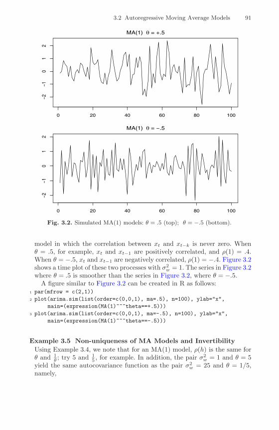
3.2 Autoregressive Moving Average Models 91
MA(1) = +.5
0 20 40 60 80 100
−2−1
01
2
MA(1) = −.5
0 20 40 60 80 100
−2−1
01
2
Fig. 3.2. Simulated MA(1) models: θ = .5 (top); θ = −.5 (bottom).
model in which the correlation between xt and xt−k is never zero. Whenθ = .5, for example, xt and xt−1 are positively correlated, and ρ(1) = .4.When θ = −.5, xt and xt−1 are negatively correlated, ρ(1) = −.4. Figure 3.2shows a time plot of these two processes with σ2
w = 1. The series in Figure 3.2where θ = .5 is smoother than the series in Figure 3.2, where θ = −.5.
A figure similar to Figure 3.2 can be created in R as follows:1 par(mfrow = c(2,1))
2 plot(arima.sim(list(order=c(0,0,1), ma=.5), n=100), ylab="x",
main=(expression(MA(1)~~~theta==+.5)))
3 plot(arima.sim(list(order=c(0,0,1), ma=-.5), n=100), ylab="x",
main=(expression(MA(1)~~~theta==-.5)))
Example 3.5 Non-uniqueness of MA Models and Invertibility
Using Example 3.4, we note that for an MA(1) model, ρ(h) is the same forθ and 1
θ ; try 5 and 15 , for example. In addition, the pair σ2
w = 1 and θ = 5yield the same autocovariance function as the pair σ2
w = 25 and θ = 1/5,namely,

92 3 ARIMA Models
γ(h) =
26 h = 0,
5 h = 1,
0 h > 1.
Thus, the MA(1) processes
xt = wt + 15wt−1, wt ∼ iid N(0, 25)
andyt = vt + 5vt−1, vt ∼ iid N(0, 1)
are the same because of normality (i.e., all finite distributions are the same).We can only observe the time series, xt or yt, and not the noise, wt or vt,so we cannot distinguish between the models. Hence, we will have to chooseonly one of them. For convenience, by mimicking the criterion of causalityfor AR models, we will choose the model with an infinite AR representation.Such a process is called an invertible process.
To discover which model is the invertible model, we can reverse the rolesof xt and wt (because we are mimicking the AR case) and write the MA(1)model as wt = −θwt−1 + xt. Following the steps that led to (3.6), if |θ| < 1,then wt =
∑∞j=0(−θ)jxt−j , which is the desired infinite AR representation
of the model. Hence, given a choice, we will choose the model with σ2w = 25
and θ = 1/5 because it is invertible.
As in the AR case, the polynomial, θ(z), corresponding to the movingaverage operators, θ(B), will be useful in exploring general properties of MAprocesses. For example, following the steps of equations (3.12)–(3.15), we canwrite the MA(1) model as xt = θ(B)wt, where θ(B) = 1 + θB. If |θ| < 1,then we can write the model as π(B)xt = wt, where π(B) = θ−1(B). Letθ(z) = 1 + θz, for |z| ≤ 1, then π(z) = θ−1(z) = 1/(1 + θz) =
∑∞j=0(−θ)jzj ,
and we determine that π(B) =∑∞j=0(−θ)jBj .
Autoregressive Moving Average Models
We now proceed with the general development of autoregressive, moving aver-age, and mixed autoregressive moving average (ARMA), models for stationarytime series.
Definition 3.5 A time series {xt; t = 0,±1,±2, . . .} is ARMA(p, q) if it isstationary and
xt = φ1xt−1 + · · ·+ φpxt−p + wt + θ1wt−1 + · · ·+ θqwt−q, (3.19)
with φp 6= 0, θq 6= 0, and σ2w > 0. The parameters p and q are called the
autoregressive and the moving average orders, respectively. If xt has a nonzeromean µ, we set α = µ(1− φ1 − · · · − φp) and write the model as
xt = α+ φ1xt−1 + · · ·+ φpxt−p + wt + θ1wt−1 + · · ·+ θqwt−q. (3.20)

3.2 Autoregressive Moving Average Models 93
Although it is not necessary yet, we assume that wt is a Gaussian white noiseseries with mean zero and variance σ2
w, unless otherwise stated.
As previously noted, when q = 0, the model is called an autoregressivemodel of order p, AR(p), and when p = 0, the model is called a moving averagemodel of order q, MA(q). To aid in the investigation of ARMA models, it willbe useful to write them using the AR operator, (3.5), and the MA operator,(3.18). In particular, the ARMA(p, q) model in (3.19) can then be written inconcise form as
φ(B)xt = θ(B)wt. (3.21)
Before we discuss the conditions under which (3.19) is causal and invertible,we point out a potential problem with the ARMA model.
Example 3.6 Parameter Redundancy
Consider a white noise process xt = wt. Equivalently, we can write this as.5xt−1 = .5wt−1 by shifting back one unit of time and multiplying by .5.Now, subtract the two representations to obtain
xt − .5xt−1 = wt − .5wt−1,
orxt = .5xt−1 − .5wt−1 + wt, (3.22)
which looks like an ARMA(1, 1) model. Of course, xt is still white noise;nothing has changed in this regard [i.e., xt = wt is the solution to (3.22)],but we have hidden the fact that xt is white noise because of the parameterredundancy or over-parameterization. Write the parameter redundant modelin operator form as φ(B)xt = θ(B)wt, or
(1− .5B)xt = (1− .5B)wt.
Apply the operator φ(B)−1 = (1− .5B)−1 to both sides to obtain
xt = (1− .5B)−1(1− .5B)xt = (1− .5B)−1(1− .5B)wt = wt,
which is the original model. We can easily detect the problem of over-parameterization with the use of the operators or their associated polynomi-als. That is, write the AR polynomial φ(z) = (1− .5z), the MA polynomialθ(z) = (1 − .5z), and note that both polynomials have a common factor,namely (1 − .5z). This common factor immediately identifies the parame-ter redundancy. Discarding the common factor in each leaves φ(z) = 1 andθ(z) = 1, from which we conclude φ(B) = 1 and θ(B) = 1, and we de-duce that the model is actually white noise. The consideration of parameterredundancy will be crucial when we discuss estimation for general ARMAmodels. As this example points out, we might fit an ARMA(1, 1) model towhite noise data and find that the parameter estimates are significant. Ifwe were unaware of parameter redundancy, we might claim the data arecorrelated when in fact they are not (Problem 3.20).
94 3 ARIMA Models
Examples 3.2, 3.5, and 3.6 point to a number of problems with the generaldefinition of ARMA(p, q) models, as given by (3.19), or, equivalently, by (3.21).To summarize, we have seen the following problems:
(i) parameter redundant models,(ii) stationary AR models that depend on the future, and
(iii) MA models that are not unique.
To overcome these problems, we will require some additional restrictionson the model parameters. First, we make the following definitions.
Definition 3.6 The AR and MA polynomials are defined as
φ(z) = 1− φ1z − · · · − φpzp, φp 6= 0, (3.23)
andθ(z) = 1 + θ1z + · · ·+ θqz
q, θq 6= 0, (3.24)
respectively, where z is a complex number.
To address the first problem, we will henceforth refer to an ARMA(p, q)model to mean that it is in its simplest form. That is, in addition to theoriginal definition given in equation (3.19), we will also require that φ(z)and θ(z) have no common factors. So, the process, xt = .5xt−1− .5wt−1 +wt,discussed in Example 3.6 is not referred to as an ARMA(1, 1) process because,in its reduced form, xt is white noise.
To address the problem of future-dependent models, we formally introducethe concept of causality.
Definition 3.7 An ARMA(p, q) model is said to be causal, if the time series{xt; t = 0,±1,±2, . . .} can be written as a one-sided linear process:
xt =∞∑j=0
ψjwt−j = ψ(B)wt, (3.25)
where ψ(B) =∑∞j=0 ψjB
j, and∑∞j=0 |ψj | <∞; we set ψ0 = 1.
In Example 3.2, the AR(1) process, xt = φxt−1 + wt, is causal only when|φ| < 1. Equivalently, the process is causal only when the root of φ(z) = 1−φzis bigger than one in absolute value. That is, the root, say, z0, of φ(z) isz0 = 1/φ (because φ(z0) = 0) and |z0| > 1 because |φ| < 1. In general, wehave the following property.
Property 3.1 Causality of an ARMA(p, q) ProcessAn ARMA(p, q) model is causal if and only if φ(z) 6= 0 for |z| ≤ 1. The
coefficients of the linear process given in (3.25) can be determined by solving
ψ(z) =
∞∑j=0
ψjzj =
θ(z)
φ(z), |z| ≤ 1.

3.2 Autoregressive Moving Average Models 95
Another way to phrase Property 3.1 is that an ARMA process is causalonly when the roots of φ(z) lie outside the unit circle; that is, φ(z) = 0only when |z| > 1. Finally, to address the problem of uniqueness discussedin Example 3.5, we choose the model that allows an infinite autoregressiverepresentation.
Definition 3.8 An ARMA(p, q) model is said to be invertible, if the timeseries {xt; t = 0,±1,±2, . . .} can be written as
π(B)xt =
∞∑j=0
πjxt−j = wt, (3.26)
where π(B) =∑∞j=0 πjB
j, and∑∞j=0 |πj | <∞; we set π0 = 1.
Analogous to Property 3.1, we have the following property.
Property 3.2 Invertibility of an ARMA(p, q) ProcessAn ARMA(p, q) model is invertible if and only if θ(z) 6= 0 for |z| ≤ 1. The
coefficients πj of π(B) given in (3.26) can be determined by solving
π(z) =
∞∑j=0
πjzj =
φ(z)
θ(z), |z| ≤ 1.
Another way to phrase Property 3.2 is that an ARMA process is invertibleonly when the roots of θ(z) lie outside the unit circle; that is, θ(z) = 0 onlywhen |z| > 1. The proof of Property 3.1 is given in Appendix B (the proof ofProperty 3.2 is similar and, hence, is not provided). The following examplesillustrate these concepts.
Example 3.7 Parameter Redundancy, Causality, Invertibility
Consider the process
xt = .4xt−1 + .45xt−2 + wt + wt−1 + .25wt−2,
or, in operator form,
(1− .4B − .45B2)xt = (1 +B + .25B2)wt.
At first, xt appears to be an ARMA(2, 2) process. But, the associatedpolynomials
φ(z) = 1− .4z − .45z2 = (1 + .5z)(1− .9z)
θ(z) = (1 + z + .25z2) = (1 + .5z)2
have a common factor that can be canceled. After cancellation, the poly-nomials become φ(z) = (1 − .9z) and θ(z) = (1 + .5z), so the model is anARMA(1, 1) model, (1− .9B)xt = (1 + .5B)wt, or
96 3 ARIMA Models
xt = .9xt−1 + .5wt−1 + wt. (3.27)
The model is causal because φ(z) = (1 − .9z) = 0 when z = 10/9, whichis outside the unit circle. The model is also invertible because the root ofθ(z) = (1 + .5z) is z = −2, which is outside the unit circle.
To write the model as a linear process, we can obtain the ψ-weights usingProperty 3.1, φ(z)ψ(z) = θ(z), or
(1− .9z)(ψ0 + ψ1z + ψ2z2 + · · · ) = (1 + .5z).
Matching coefficients we get ψ0 = 1, ψ1 = .5 + .9 = 1.4, and ψj = .9ψj−1for j > 1. Thus, ψj = 1.4(.9)j−1 for j ≥ 1 and (3.27) can be written as
xt = wt + 1.4∞∑j=1
.9j−1wt−j .
Similarly, the invertible representation using Property 3.2 is
xt = 1.4∞∑j=1
(−.5)j−1xt−j + wt.
Example 3.8 Causal Conditions for an AR(2) Process
For an AR(1) model, (1−φB)xt = wt, to be causal, the root of φ(z) = 1−φzmust lie outside of the unit circle. In this case, the root (or zero) occurs atz0 = 1/φ [i.e., φ(z0) = 0], so it is easy to go from the causal requirement onthe root, |1/φ| > 1, to a requirement on the parameter, |φ| < 1. It is not soeasy to establish this relationship for higher order models.
For example, the AR(2) model, (1− φ1B − φ2B2)xt = wt, is causal whenthe two roots of φ(z) = 1 − φ1z − φ2z2 lie outside of the unit circle. Usingthe quadratic formula, this requirement can be written as∣∣∣∣∣φ1 ±
√φ21 + 4φ2−2φ2
∣∣∣∣∣ > 1.
The roots of φ(z) may be real and distinct, real and equal, or a complexconjugate pair. If we denote those roots by z1 and z2, we can write φ(z) =(1−z−11 z)(1−z−12 z); note that φ(z1) = φ(z2) = 0. The model can be writtenin operator form as (1−z−11 B)(1−z−12 B)xt = wt. From this representation,it follows that φ1 = (z−11 + z−12 ) and φ2 = −(z1z2)−1. This relationship andthe fact that |z1| > 1 and |z2| > 1 can be used to establish the followingequivalent condition for causality:
φ1 + φ2 < 1, φ2 − φ1 < 1, and |φ2| < 1. (3.28)
This causality condition specifies a triangular region in the parameter space.We leave the details of the equivalence to the reader (Problem 3.5).

3.3 Difference Equations 97
3.3 Difference Equations
The study of the behavior of ARMA processes and their ACFs is greatlyenhanced by a basic knowledge of difference equations, simply because theyare difference equations. This topic is also useful in the study of time domainmodels and stochastic processes in general. We will give a brief and heuristicaccount of the topic along with some examples of the usefulness of the theory.For details, the reader is referred to Mickens (1990).
Suppose we have a sequence of numbers u0, u1, u2, . . . such that
un − αun−1 = 0, α 6= 0, n = 1, 2, . . . . (3.29)
For example, recall (3.9) in which we showed that the ACF of an AR(1)process is a sequence, ρ(h), satisfying
ρ(h)− φρ(h− 1) = 0, h = 1, 2, . . . .
Equation (3.29) represents a homogeneous difference equation of order 1. Tosolve the equation, we write:
u1 = αu0
u2 = αu1 = α2u0...
un = αun−1 = αnu0.
Given an initial condition u0 = c, we may solve (3.29), namely, un = αnc.In operator notation, (3.29) can be written as (1− αB)un = 0. The poly-
nomial associated with (3.29) is α(z) = 1 − αz, and the root, say, z0, of thispolynomial is z0 = 1/α; that is α(z0) = 0. We know a solution (in fact, thesolution) to (3.29), with initial condition u0 = c, is
un = αnc =(z−10
)nc. (3.30)
That is, the solution to the difference equation (3.29) depends only on theinitial condition and the inverse of the root to the associated polynomial α(z).
Now suppose that the sequence satisfies
un − α1un−1 − α2un−2 = 0, α2 6= 0, n = 2, 3, . . . (3.31)
This equation is a homogeneous difference equation of order 2. The corre-sponding polynomial is
α(z) = 1− α1z − α2z2,
which has two roots, say, z1 and z2; that is, α(z1) = α(z2) = 0. We willconsider two cases. First suppose z1 6= z2. Then the general solution to (3.31)is
98 3 ARIMA Models
un = c1z−n1 + c2z
−n2 , (3.32)
where c1 and c2 depend on the initial conditions. The claim that is a solutioncan be verified by direct substitution of (3.32) into (3.31):(c1z−n1 + c2z
−n2
)− α1
(c1z−(n−1)1 + c2z
−(n−1)2
)− α2
(c1z−(n−2)1 + c2z
−(n−2)2
)= c1z
−n1
(1− α1z1 − α2z
21
)+ c2z
−n2
(1− α1z2 − α2z
22
)= c1z
−n1 α(z1) + c2z
−n2 α(z2) = 0.
Given two initial conditions u0 and u1, we may solve for c1 and c2:
u0 = c1 + c2 and u1 = c1z−11 + c2z
−12 ,
where z1 and z2 can be solved for in terms of α1 and α2 using the quadraticformula, for example.
When the roots are equal, z1 = z2 (= z0), a general solution to (3.31) is
un = z−n0 (c1 + c2n). (3.33)
This claim can also be verified by direct substitution of (3.33) into (3.31):
z−n0 (c1 + c2n)− α1
(z−(n−1)0 [c1 + c2(n− 1)]
)− α2
(z−(n−2)0 [c1 + c2(n− 2)]
)= z−n0 (c1 + c2n)
(1− α1z0 − α2z
20
)+ c2z
−n+10 (α1 + 2α2z0)
= c2z−n+10 (α1 + 2α2z0) .
To show that (α1 + 2α2z0) = 0, write 1 − α1z − α2z2 = (1 − z−10 z)2, and
take derivatives with respect to z on both sides of the equation to obtain(α1 + 2α2z) = 2z−10 (1 − z−10 z). Thus, (α1 + 2α2z0) = 2z−10 (1 − z−10 z0) = 0,as was to be shown. Finally, given two initial conditions, u0 and u1, we cansolve for c1 and c2:
u0 = c1 and u1 = (c1 + c2)z−10 .
It can also be shown that these solutions are unique.To summarize these results, in the case of distinct roots, the solution to
the homogeneous difference equation of degree two was
un = z−n1 × (a polynomial in n of degree m1 − 1)
+ z−n2 × (a polynomial in n of degree m2 − 1),(3.34)
wherem1 is the multiplicity of the root z1 andm2 is the multiplicity of the rootz2. In this example, of course, m1 = m2 = 1, and we called the polynomialsof degree zero c1 and c2, respectively. In the case of the repeated root, thesolution was
un = z−n0 × (a polynomial in n of degree m0 − 1), (3.35)
where m0 is the multiplicity of the root z0; that is, m0 = 2. In this case, wewrote the polynomial of degree one as c1 + c2n. In both cases, we solved forc1 and c2 given two initial conditions, u0 and u1.

3.3 Difference Equations 99
Example 3.9 The ACF of an AR(2) Process
Suppose xt = φ1xt−1 +φ2xt−2 +wt is a causal AR(2) process. Multiply eachside of the model by xt−h for h > 0, and take expectation:
E(xtxt−h) = φ1E(xt−1xt−h) + φ2E(xt−2xt−h) + E(wtxt−h).
The result is
γ(h) = φ1γ(h− 1) + φ2γ(h− 2), h = 1, 2, . . . . (3.36)
In (3.36), we used the fact that E(xt) = 0 and for h > 0,
E(wtxt−h) = E(wt
∞∑j=0
ψjwt−h−j
)= 0.
Divide (3.36) through by γ(0) to obtain the difference equation for the ACFof the process:
ρ(h)− φ1ρ(h− 1)− φ2ρ(h− 2) = 0, h = 1, 2, . . . . (3.37)
The initial conditions are ρ(0) = 1 and ρ(−1) = φ1/(1 − φ2), which isobtained by evaluating (3.37) for h = 1 and noting that ρ(1) = ρ(−1).
Using the results for the homogeneous difference equation of order two, letz1 and z2 be the roots of the associated polynomial, φ(z) = 1− φ1z − φ2z2.Because the model is causal, we know the roots are outside the unit circle:|z1| > 1 and |z2| > 1. Now, consider the solution for three cases:(i) When z1 and z2 are real and distinct, then
ρ(h) = c1z−h1 + c2z
−h2 ,
so ρ(h)→ 0 exponentially fast as h→∞.(ii) When z1 = z2 (= z0) are real and equal, then
ρ(h) = z−h0 (c1 + c2h),
so ρ(h)→ 0 exponentially fast as h→∞.(iii) When z1 = z2 are a complex conjugate pair, then c2 = c1 (because ρ(h)
is real), andρ(h) = c1z
−h1 + c1z
−h1 .
Write c1 and z1 in polar coordinates, for example, z1 = |z1|eiθ, where θis the angle whose tangent is the ratio of the imaginary part and the realpart of z1 (sometimes called arg(z1); the range of θ is [−π, π]). Then,using the fact that eiα + e−iα = 2 cos(α), the solution has the form
ρ(h) = a|z1|−h cos(hθ + b),
where a and b are determined by the initial conditions. Again, ρ(h)dampens to zero exponentially fast as h → ∞, but it does so in a si-nusoidal fashion. The implication of this result is shown in the nextexample.
100 3 ARIMA Models
Example 3.10 An AR(2) with Complex Roots
Figure 3.3 shows n = 144 observations from the AR(2) model
xt = 1.5xt−1 − .75xt−2 + wt,
with σ2w = 1, and with complex roots chosen so the process exhibits pseudo-
cyclic behavior at the rate of one cycle every 12 time points. The autore-gressive polynomial for this model is φ(z) = 1 − 1.5z + .75z2. The roots ofφ(z) are 1± i/
√3, and θ = tan−1(1/
√3) = 2π/12 radians per unit time. To
convert the angle to cycles per unit time, divide by 2π to get 1/12 cyclesper unit time. The ACF for this model is shown in §3.4, Figure 3.4.
To calculate the roots of the polynomial and solve for arg in R:1 z = c(1,-1.5,.75) # coefficients of the polynomial
2 (a = polyroot(z)[1]) # print one root: 1+0.57735i = 1 + i/sqrt(3)
3 arg = Arg(a)/(2*pi) # arg in cycles/pt
4 1/arg # = 12, the pseudo period
To reproduce Figure 3.3:1 set.seed(90210)
2 ar2 = arima.sim(list(order=c(2,0,0), ar=c(1.5,-.75)), n = 144)
3 plot(1:144/12, ar2, type="l", xlab="Time (one unit = 12 points)")
4 abline(v=0:12, lty="dotted", lwd=2)
To calculate and display the ACF for this model:1 ACF = ARMAacf(ar=c(1.5,-.75), ma=0, 50)
2 plot(ACF, type="h", xlab="lag")
3 abline(h=0)
We now exhibit the solution for the general homogeneous difference equa-tion of order p:
un − α1un−1 − · · · − αpun−p = 0, αp 6= 0, n = p, p+ 1, . . . . (3.38)
The associated polynomial is
α(z) = 1− α1z − · · · − αpzp.
Suppose α(z) has r distinct roots, z1 with multiplicity m1, z2 with multiplicitym2, . . . , and zr with multiplicity mr, such that m1 +m2 + · · ·+mr = p. Thegeneral solution to the difference equation (3.38) is
un = z−n1 P1(n) + z−n2 P2(n) + · · ·+ z−nr Pr(n), (3.39)
where Pj(n), for j = 1, 2, . . . , r, is a polynomial in n, of degree mj − 1. Givenp initial conditions u0, . . . , up−1, we can solve for the Pj(n) explicitly.
Example 3.11 The ψψψ-weights for an ARMA Model
For a causal ARMA(p, q) model, φ(B)xt = θ(B)wt, where the zeros of φ(z)are outside the unit circle, recall that we may write

3.3 Difference Equations 101
0 2 4 6 8 10 12
−50
5
Time (one unit = 12 points)
ar2
Fig. 3.3. Simulated AR(2) model, n = 144 with φ1 = 1.5 and φ2 = −.75.
xt =∞∑j=0
ψjwt−j ,
where the ψ-weights are determined using Property 3.1.For the pure MA(q) model, ψ0 = 1, ψj = θj , for j = 1, . . . , q, and ψj = 0,
otherwise. For the general case of ARMA(p, q) models, the task of solvingfor the ψ-weights is much more complicated, as was demonstrated in Exam-ple 3.7. The use of the theory of homogeneous difference equations can helphere. To solve for the ψ-weights in general, we must match the coefficientsin φ(z)ψ(z) = θ(z):
(1− φ1z − φ2z2 − · · · )(ψ0 + ψ1z + ψ2z2 + · · · ) = (1 + θ1z + θ2z
2 + · · · ).
The first few values are
ψ0 = 1ψ1 − φ1ψ0 = θ1
ψ2 − φ1ψ1 − φ2ψ0 = θ2ψ3 − φ1ψ2 − φ2ψ1 − φ3ψ0 = θ3
...
where we would take φj = 0 for j > p, and θj = 0 for j > q. The ψ-weightssatisfy the homogeneous difference equation given by
ψj −p∑k=1
φkψj−k = 0, j ≥ max(p, q + 1), (3.40)
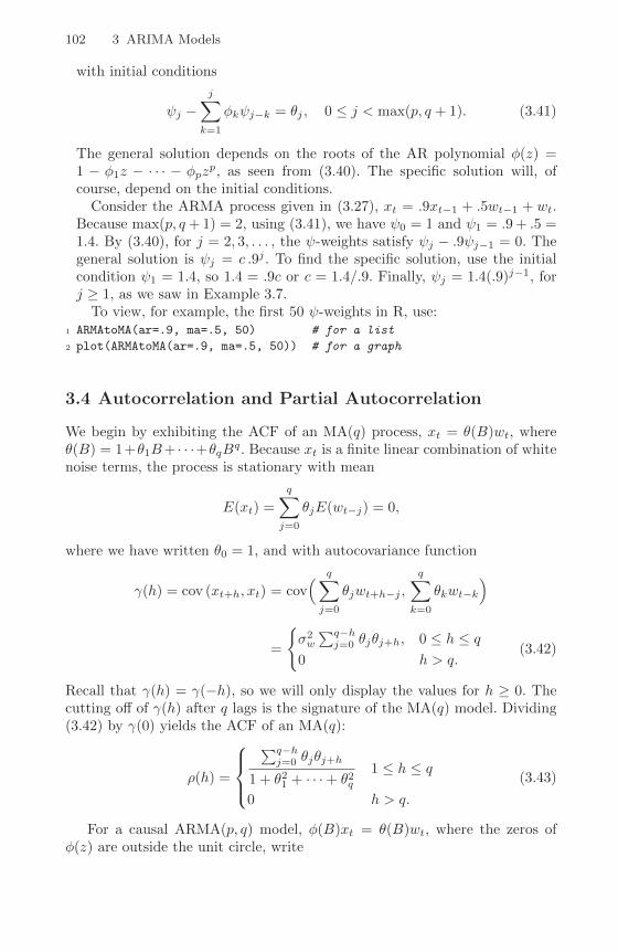
102 3 ARIMA Models
with initial conditions
ψj −j∑
k=1
φkψj−k = θj , 0 ≤ j < max(p, q + 1). (3.41)
The general solution depends on the roots of the AR polynomial φ(z) =1 − φ1z − · · · − φpz
p, as seen from (3.40). The specific solution will, ofcourse, depend on the initial conditions.
Consider the ARMA process given in (3.27), xt = .9xt−1 + .5wt−1 + wt.Because max(p, q+ 1) = 2, using (3.41), we have ψ0 = 1 and ψ1 = .9 + .5 =1.4. By (3.40), for j = 2, 3, . . . , the ψ-weights satisfy ψj − .9ψj−1 = 0. Thegeneral solution is ψj = c .9j . To find the specific solution, use the initialcondition ψ1 = 1.4, so 1.4 = .9c or c = 1.4/.9. Finally, ψj = 1.4(.9)j−1, forj ≥ 1, as we saw in Example 3.7.
To view, for example, the first 50 ψ-weights in R, use:1 ARMAtoMA(ar=.9, ma=.5, 50) # for a list
2 plot(ARMAtoMA(ar=.9, ma=.5, 50)) # for a graph
3.4 Autocorrelation and Partial Autocorrelation
We begin by exhibiting the ACF of an MA(q) process, xt = θ(B)wt, whereθ(B) = 1+θ1B+ · · ·+θqB
q. Because xt is a finite linear combination of whitenoise terms, the process is stationary with mean
E(xt) =
q∑j=0
θjE(wt−j) = 0,
where we have written θ0 = 1, and with autocovariance function
γ(h) = cov (xt+h, xt) = cov( q∑j=0
θjwt+h−j ,
q∑k=0
θkwt−k
)
=
{σ2w
∑q−hj=0 θjθj+h, 0 ≤ h ≤ q
0 h > q.(3.42)
Recall that γ(h) = γ(−h), so we will only display the values for h ≥ 0. Thecutting off of γ(h) after q lags is the signature of the MA(q) model. Dividing(3.42) by γ(0) yields the ACF of an MA(q):
ρ(h) =
∑q−hj=0 θjθj+h
1 + θ21 + · · ·+ θ2q1 ≤ h ≤ q
0 h > q.
(3.43)
For a causal ARMA(p, q) model, φ(B)xt = θ(B)wt, where the zeros ofφ(z) are outside the unit circle, write
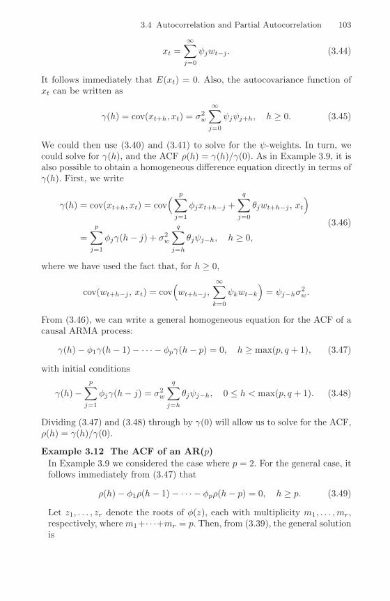
3.4 Autocorrelation and Partial Autocorrelation 103
xt =
∞∑j=0
ψjwt−j . (3.44)
It follows immediately that E(xt) = 0. Also, the autocovariance function ofxt can be written as
γ(h) = cov(xt+h, xt) = σ2w
∞∑j=0
ψjψj+h, h ≥ 0. (3.45)
We could then use (3.40) and (3.41) to solve for the ψ-weights. In turn, wecould solve for γ(h), and the ACF ρ(h) = γ(h)/γ(0). As in Example 3.9, it isalso possible to obtain a homogeneous difference equation directly in terms ofγ(h). First, we write
γ(h) = cov(xt+h, xt) = cov( p∑j=1
φjxt+h−j +
q∑j=0
θjwt+h−j , xt
)=
p∑j=1
φjγ(h− j) + σ2w
q∑j=h
θjψj−h, h ≥ 0,
(3.46)
where we have used the fact that, for h ≥ 0,
cov(wt+h−j , xt) = cov(wt+h−j ,
∞∑k=0
ψkwt−k
)= ψj−hσ
2w.
From (3.46), we can write a general homogeneous equation for the ACF of acausal ARMA process:
γ(h)− φ1γ(h− 1)− · · · − φpγ(h− p) = 0, h ≥ max(p, q + 1), (3.47)
with initial conditions
γ(h)−p∑j=1
φjγ(h− j) = σ2w
q∑j=h
θjψj−h, 0 ≤ h < max(p, q + 1). (3.48)
Dividing (3.47) and (3.48) through by γ(0) will allow us to solve for the ACF,ρ(h) = γ(h)/γ(0).
Example 3.12 The ACF of an AR(p)
In Example 3.9 we considered the case where p = 2. For the general case, itfollows immediately from (3.47) that
ρ(h)− φ1ρ(h− 1)− · · · − φpρ(h− p) = 0, h ≥ p. (3.49)
Let z1, . . . , zr denote the roots of φ(z), each with multiplicity m1, . . . ,mr,respectively, where m1+· · ·+mr = p. Then, from (3.39), the general solutionis
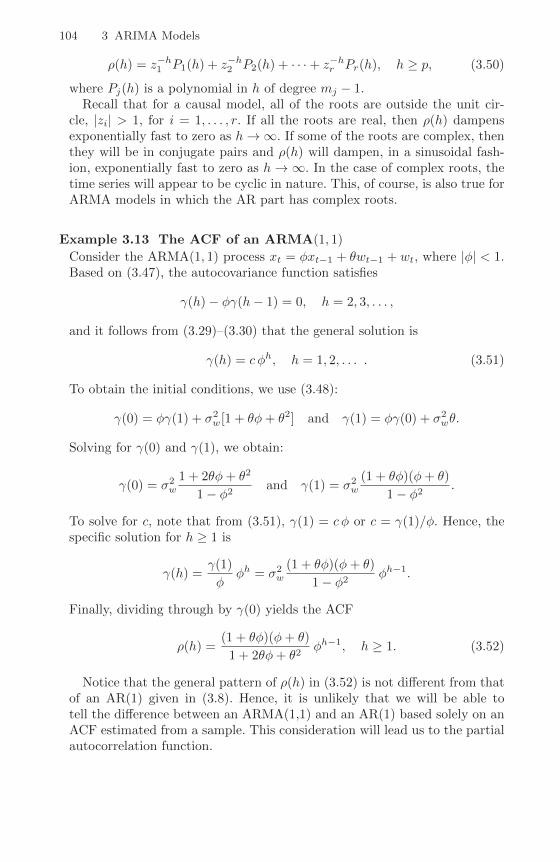
104 3 ARIMA Models
ρ(h) = z−h1 P1(h) + z−h2 P2(h) + · · ·+ z−hr Pr(h), h ≥ p, (3.50)
where Pj(h) is a polynomial in h of degree mj − 1.Recall that for a causal model, all of the roots are outside the unit cir-
cle, |zi| > 1, for i = 1, . . . , r. If all the roots are real, then ρ(h) dampensexponentially fast to zero as h→∞. If some of the roots are complex, thenthey will be in conjugate pairs and ρ(h) will dampen, in a sinusoidal fash-ion, exponentially fast to zero as h→∞. In the case of complex roots, thetime series will appear to be cyclic in nature. This, of course, is also true forARMA models in which the AR part has complex roots.
Example 3.13 The ACF of an ARMA(1, 1)
Consider the ARMA(1, 1) process xt = φxt−1 + θwt−1 + wt, where |φ| < 1.Based on (3.47), the autocovariance function satisfies
γ(h)− φγ(h− 1) = 0, h = 2, 3, . . . ,
and it follows from (3.29)–(3.30) that the general solution is
γ(h) = c φh, h = 1, 2, . . . . (3.51)
To obtain the initial conditions, we use (3.48):
γ(0) = φγ(1) + σ2w[1 + θφ+ θ2] and γ(1) = φγ(0) + σ2
wθ.
Solving for γ(0) and γ(1), we obtain:
γ(0) = σ2w
1 + 2θφ+ θ2
1− φ2and γ(1) = σ2
w
(1 + θφ)(φ+ θ)
1− φ2.
To solve for c, note that from (3.51), γ(1) = c φ or c = γ(1)/φ. Hence, thespecific solution for h ≥ 1 is
γ(h) =γ(1)
φφh = σ2
w
(1 + θφ)(φ+ θ)
1− φ2φh−1.
Finally, dividing through by γ(0) yields the ACF
ρ(h) =(1 + θφ)(φ+ θ)
1 + 2θφ+ θ2φh−1, h ≥ 1. (3.52)
Notice that the general pattern of ρ(h) in (3.52) is not different from thatof an AR(1) given in (3.8). Hence, it is unlikely that we will be able totell the difference between an ARMA(1,1) and an AR(1) based solely on anACF estimated from a sample. This consideration will lead us to the partialautocorrelation function.

3.4 Autocorrelation and Partial Autocorrelation 105
The Partial Autocorrelation Function (PACF)
We have seen in (3.43), for MA(q) models, the ACF will be zero for lagsgreater than q. Moreover, because θq 6= 0, the ACF will not be zero at lagq. Thus, the ACF provides a considerable amount of information about theorder of the dependence when the process is a moving average process. If theprocess, however, is ARMA or AR, the ACF alone tells us little about theorders of dependence. Hence, it is worthwhile pursuing a function that willbehave like the ACF of MA models, but for AR models, namely, the partialautocorrelation function (PACF).
To motivate the idea, consider a causal AR(1) model, xt = φxt−1 + wt.Then,
γx(2) = cov(xt, xt−2) = cov(φxt−1 + wt, xt−2)
= cov(φ2xt−2 + φwt−1 + wt, xt−2) = φ2γx(0).
This result follows from causality because xt−2 involves {wt−2, wt−3, . . .},which are all uncorrelated with wt and wt−1. The correlation between xtand xt−2 is not zero, as it would be for an MA(1), because xt is dependent onxt−2 through xt−1. Suppose we break this chain of dependence by removing(or partial out) the effect xt−1. That is, we consider the correlation betweenxt − φxt−1 and xt−2 − φxt−1, because it is the correlation between xt andxt−2 with the linear dependence of each on xt−1 removed. In this way, wehave broken the dependence chain between xt and xt−2. In fact,
cov(xt − φxt−1, xt−2 − φxt−1) = cov(wt, xt−2 − φxt−1) = 0.
Hence, the tool we need is partial autocorrelation, which is the correlationbetween xs and xt with the linear effect of everything “in the middle” removed.
To formally define the PACF for mean-zero stationary time series, let xt+h,for h ≥ 2, denote the regression3 of xt+h on {xt+h−1, xt+h−2, . . . , xt+1}, whichwe write as
xt+h = β1xt+h−1 + β2xt+h−2 + · · ·+ βh−1xt+1. (3.53)
No intercept term is needed in (3.53) because the mean of xt is zero (other-wise, replace xt by xt − µx in this discussion). In addition, let xt denote theregression of xt on {xt+1, xt+2, . . . , xt+h−1}, then
xt = β1xt+1 + β2xt+2 + · · ·+ βh−1xt+h−1. (3.54)
Because of stationarity, the coefficients, β1, . . . , βh−1 are the same in (3.53)and (3.54); we will explain this result in the next section.
3 The term regression here refers to regression in the population sense. That is,xt+h is the linear combination of {xt+h−1, xt+h−2, . . . , xt+1} that minimizes themean squared error E(xt+h −
∑h−1j=1 αjxt+j)
2.

106 3 ARIMA Models
Definition 3.9 The partial autocorrelation function (PACF) of a sta-tionary process, xt, denoted φhh, for h = 1, 2, . . . , is
φ11 = corr(xt+1, xt) = ρ(1) (3.55)
andφhh = corr(xt+h − xt+h, xt − xt), h ≥ 2. (3.56)
Both (xt+h−xt+h) and (xt−xt) are uncorrelated with {xt+1, . . . , xt+h−1}.The PACF, φhh, is the correlation between xt+h and xt with the linear depen-dence of {xt+1, . . . , xt+h−1} on each, removed. If the process xt is Gaussian,then φhh = corr(xt+h, xt | xt+1, . . . , xt+h−1); that is, φhh is the correlationcoefficient between xt+h and xt in the bivariate distribution of (xt+h, xt) con-ditional on {xt+1, . . . , xt+h−1}.
Example 3.14 The PACF of an AR(1)
Consider the PACF of the AR(1) process given by xt = φxt−1 + wt, with|φ| < 1. By definition, φ11 = ρ(1) = φ. To calculate φ22, consider theregression of xt+2 on xt+1, say, xt+2 = βxt+1. We choose β to minimize
E(xt+2 − xt+2)2 = E(xt+2 − βxt+1)2 = γ(0)− 2βγ(1) + β2γ(0).
Taking derivatives with respect to β and setting the result equal to zero, wehave β = γ(1)/γ(0) = ρ(1) = φ. Next, consider the regression of xt on xt+1,say xt = βxt+1. We choose β to minimize
E(xt − xt)2 = E(xt − βxt+1)2 = γ(0)− 2βγ(1) + β2γ(0).
This is the same equation as before, so β = φ. Hence,
φ22 = corr(xt+2 − xt+2, xt − xt) = corr(xt+2 − φxt+1, xt − φxt+1)
= corr(wt+2, xt − φxt+1) = 0
by causality. Thus, φ22 = 0. In the next example, we will see that in thiscase, φhh = 0 for all h > 1.
Example 3.15 The PACF of an AR(p)
The model implies xt+h =∑pj=1 φjxt+h−j + wt+h, where the roots of
φ(z) are outside the unit circle. When h > p, the regression of xt+h on{xt+1, . . . , xt+h−1}, is
xt+h =
p∑j=1
φjxt+h−j .
We have not proved this obvious result yet, but we will prove it in the nextsection. Thus, when h > p,
φhh = corr(xt+h − xt+h, xt − xt) = corr(wt+h, xt − xt) = 0,

3.4 Autocorrelation and Partial Autocorrelation 107
5 10 15 20
−0.5
0.0
0.5
1.0
lag
AC
F
5 10 15 20
−0.5
0.0
0.5
1.0
lag
PA
CF
Fig. 3.4. The ACF and PACF of an AR(2) model with φ1 = 1.5 and φ2 = −.75.
because, by causality, xt − xt depends only on {wt+h−1, wt+h−2, . . .}; recallequation (3.54). When h ≤ p, φpp is not zero, and φ11, . . . , φp−1,p−1 are notnecessarily zero. We will see later that, in fact, φpp = φp. Figure 3.4 showsthe ACF and the PACF of the AR(2) model presented in Example 3.10.
To reproduce Figure 3.4 in R, use the following commands:1 ACF = ARMAacf(ar=c(1.5,-.75), ma=0, 24)[-1]
2 PACF = ARMAacf(ar=c(1.5,-.75), ma=0, 24, pacf=TRUE)
3 par(mfrow=c(1,2))
4 plot(ACF, type="h", xlab="lag", ylim=c(-.8,1)); abline(h=0)
5 plot(PACF, type="h", xlab="lag", ylim=c(-.8,1)); abline(h=0)
Example 3.16 The PACF of an Invertible MA(q)
For an invertible MA(q), we can write xt = −∑∞j=1 πjxt−j +wt. Moreover,
no finite representation exists. From this result, it should be apparent thatthe PACF will never cut off, as in the case of an AR(p).
For an MA(1), xt = wt + θwt−1, with |θ| < 1, calculations similar toExample 3.14 will yield φ22 = −θ2/(1 + θ2 + θ4). For the MA(1) in general,we can show that
φhh = − (−θ)h(1− θ2)
1− θ2(h+1), h ≥ 1.
In the next section, we will discuss methods of calculating the PACF. ThePACF for MA models behaves much like the ACF for AR models. Also, thePACF for AR models behaves much like the ACF for MA models. Becausean invertible ARMA model has an infinite AR representation, the PACF willnot cut off. We may summarize these results in Table 3.1.

108 3 ARIMA Models
Table 3.1. Behavior of the ACF and PACF for ARMA Models
AR(p) MA(q) ARMA(p, q)
ACF Tails off Cuts off Tails offafter lag q
PACF Cuts off Tails off Tails offafter lag p
Example 3.17 Preliminary Analysis of the Recruitment Series
We consider the problem of modeling the Recruitment series shown in Fig-ure 1.5. There are 453 months of observed recruitment ranging over theyears 1950-1987. The ACF and the PACF given in Figure 3.5 are con-sistent with the behavior of an AR(2). The ACF has cycles correspond-ing roughly to a 12-month period, and the PACF has large values forh = 1, 2 and then is essentially zero for higher order lags. Based on Ta-ble 3.1, these results suggest that a second-order (p = 2) autoregres-sive model might provide a good fit. Although we will discuss estimationin detail in §3.6, we ran a regression (see §2.2) using the data triplets{(x; z1, z2) : (x3;x2, x1), (x4;x3, x2), . . . , (x453;x452, x451)} to fit a model ofthe form
xt = φ0 + φ1xt−1 + φ2xt−2 + wt
for t = 3, 4, . . . , 453. The values of the estimates were φ0 = 6.74(1.11),
φ1 = 1.35(.04), φ2 = −.46(.04), and σ2w = 89.72, where the estimated standard
errors are in parentheses.The following R code can be used for this analysis. We use the script acf2
to print and plot the ACF and PACF; see Appendix R for details.1 acf2(rec, 48) # will produce values and a graphic
2 (regr = ar.ols(rec, order=2, demean=FALSE, intercept=TRUE))
3 regr$asy.se.coef # standard errors of the estimates
3.5 Forecasting
In forecasting, the goal is to predict future values of a time series, xn+m, m =1, 2, . . ., based on the data collected to the present, xxx = {xn, xn−1, . . . , x1}.Throughout this section, we will assume xt is stationary and the model pa-rameters are known. The problem of forecasting when the model parametersare unknown will be discussed in the next section; also, see Problem 3.26. Theminimum mean square error predictor of xn+m is
xnn+m = E(xn+m∣∣ xxx) (3.57)
because the conditional expectation minimizes the mean square error
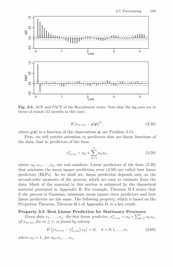
3.5 Forecasting 109
0 1 2 3 4
−0.5
0.0
0.5
1.0
LAG
ACF
0 1 2 3 4
−0.5
0.0
0.5
1.0
LAG
PACF
Fig. 3.5. ACF and PACF of the Recruitment series. Note that the lag axes are interms of season (12 months in this case).
E [xn+m − g(xxx)]2, (3.58)
where g(xxx) is a function of the observations xxx; see Problem 3.14.First, we will restrict attention to predictors that are linear functions of
the data, that is, predictors of the form
xnn+m = α0 +n∑k=1
αkxk, (3.59)
where α0, α1, . . . , αn are real numbers. Linear predictors of the form (3.59)that minimize the mean square prediction error (3.58) are called best linearpredictors (BLPs). As we shall see, linear prediction depends only on thesecond-order moments of the process, which are easy to estimate from thedata. Much of the material in this section is enhanced by the theoreticalmaterial presented in Appendix B. For example, Theorem B.3 states thatif the process is Gaussian, minimum mean square error predictors and bestlinear predictors are the same. The following property, which is based on theProjection Theorem, Theorem B.1 of Appendix B, is a key result.
Property 3.3 Best Linear Prediction for Stationary ProcessesGiven data x1, . . . , xn, the best linear predictor, xnn+m = α0 +
∑nk=1 αkxk,
of xn+m, for m ≥ 1, is found by solving
E[(xn+m − xnn+m
)xk]
= 0, k = 0, 1, . . . , n, (3.60)
where x0 = 1, for α0, α1, . . . αn.
110 3 ARIMA Models
The equations specified in (3.60) are called the prediction equations, andthey are used to solve for the coefficients {α0, α1, . . . , αn}. If E(xt) = µ, thefirst equation (k = 0) of (3.60) implies
E(xnn+m) = E(xn+m) = µ.
Thus, taking expectation in (3.59), we have
µ = α0 +n∑k=1
αkµ or α0 = µ(
1−n∑k=1
αk
).
Hence, the form of the BLP is
xnn+m = µ+n∑k=1
αk(xk − µ).
Thus, until we discuss estimation, there is no loss of generality in consideringthe case that µ = 0, in which case, α0 = 0.
First, consider one-step-ahead prediction. That is, given {x1, . . . , xn}, wewish to forecast the value of the time series at the next time point, xn+1. TheBLP of xn+1 is of the form
xnn+1 = φn1xn + φn2xn−1 + · · ·+ φnnx1, (3.61)
where, for purposes that will become clear shortly, we have written αk in(3.59), as φn,n+1−k in (3.61), for k = 1, . . . , n. Using Property 3.3, the coeffi-cients {φn1, φn2, . . . , φnn} satisfy
E[(xn+1 −
n∑j=1
φnjxn+1−j
)xn+1−k
]= 0, k = 1, . . . , n,
orn∑j=1
φnjγ(k − j) = γ(k), k = 1, . . . , n. (3.62)
The prediction equations (3.62) can be written in matrix notation as
Γnφφφn = γγγn, (3.63)
where Γn = {γ(k − j)}nj,k=1 is an n × n matrix, φφφn = (φn1, . . . , φnn)′ is an
n× 1 vector, and γγγn = (γ(1), . . . , γ(n))′
is an n× 1 vector.The matrix Γn is nonnegative definite. If Γn is singular, there are many
solutions to (3.63), but, by the Projection Theorem (Theorem B.1), xnn+1 isunique. If Γn is nonsingular, the elements of φφφn are unique, and are given by
φφφn = Γ−1n γγγn. (3.64)
3.5 Forecasting 111
For ARMA models, the fact that σ2w > 0 and γ(h)→ 0 as h→∞ is enough to
ensure that Γn is positive definite (Problem 3.12). It is sometimes convenientto write the one-step-ahead forecast in vector notation
xnn+1 = φφφ′nxxx, (3.65)
where xxx = (xn, xn−1, . . . , x1)′.The mean square one-step-ahead prediction error is
Pnn+1 = E(xn+1 − xnn+1)2 = γ(0)− γγγ′nΓ−1n γγγn. (3.66)
To verify (3.66) using (3.64) and (3.65),
E(xn+1 − xnn+1)2 = E(xn+1 − φφφ′nxxx)2 = E(xn+1 − γγγ′nΓ−1n xxx)2
= E(x2n+1 − 2γγγ′nΓ−1n xxxxn+1 + γγγ′nΓ
−1n xxxxxx′Γ−1n γγγn)
= γ(0)− 2γγγ′nΓ−1n γγγn + γγγ′nΓ
−1n ΓnΓ
−1n γγγn
= γ(0)− γγγ′nΓ−1n γγγn.
Example 3.18 Prediction for an AR(2)
Suppose we have a causal AR(2) process xt = φ1xt−1+φ2xt−2+wt, and oneobservation x1. Then, using equation (3.64), the one-step-ahead predictionof x2 based on x1 is
x12 = φ11x1 =γ(1)
γ(0)x1 = ρ(1)x1.
Now, suppose we want the one-step-ahead prediction of x3 based on twoobservations x1 and x2; i.e., x23 = φ21x2 + φ22x1. We could use (3.62)
φ21γ(0) + φ22γ(1) = γ(1)
φ21γ(1) + φ22γ(0) = γ(2)
to solve for φ21 and φ22, or use the matrix form in (3.64) and solve(φ21φ22
)=
(γ(0) γ(1)γ(1) γ(0)
)−1(γ(1)γ(2)
),
but, it should be apparent from the model that x23 = φ1x2 + φ2x1. Becauseφ1x2 + φ2x1 satisfies the prediction equations (3.60),
E{[x3 − (φ1x2 + φ2x1)]x1} = E(w3x1) = 0,
E{[x3 − (φ1x2 + φ2x1)]x2} = E(w3x2) = 0,
it follows that, indeed, x23 = φ1x2 + φ2x1, and by the uniqueness of thecoefficients in this case, that φ21 = φ1 and φ22 = φ2. Continuing in this way,it is easy to verify that, for n ≥ 2,
xnn+1 = φ1xn + φ2xn−1.
That is, φn1 = φ1, φn2 = φ2, and φnj = 0, for j = 3, 4, . . . , n.

112 3 ARIMA Models
From Example 3.18, it should be clear (Problem 3.40) that, if the timeseries is a causal AR(p) process, then, for n ≥ p,
xnn+1 = φ1xn + φ2xn−1 + · · ·+ φpxn−p+1. (3.67)
For ARMA models in general, the prediction equations will not be as simpleas the pure AR case. In addition, for n large, the use of (3.64) is prohibitivebecause it requires the inversion of a large matrix. There are, however, iterativesolutions that do not require any matrix inversion. In particular, we mentionthe recursive solution due to Levinson (1947) and Durbin (1960).
Property 3.4 The Durbin–Levinson AlgorithmEquations (3.64) and (3.66) can be solved iteratively as follows:
φ00 = 0, P 01 = γ(0). (3.68)
For n ≥ 1,
φnn =ρ(n)−
∑n−1k=1 φn−1,k ρ(n− k)
1−∑n−1k=1 φn−1,k ρ(k)
, Pnn+1 = Pn−1n (1− φ2nn), (3.69)
where, for n ≥ 2,
φnk = φn−1,k − φnnφn−1,n−k, k = 1, 2, . . . , n− 1. (3.70)
The proof of Property 3.4 is left as an exercise; see Problem 3.13.
Example 3.19 Using the Durbin–Levinson Algorithm
To use the algorithm, start with φ00 = 0, P 01 = γ(0). Then, for n = 1,
φ11 = ρ(1), P 12 = γ(0)[1− φ211].
For n = 2,
φ22 =ρ(2)− φ11 ρ(1)
1− φ11 ρ(1), φ21 = φ11 − φ22φ11,
P 23 = P 1
2 [1− φ222] = γ(0)[1− φ211][1− φ222].
For n = 3,
φ33 =ρ(3)− φ21 ρ(2)− φ22 ρ(1)
1− φ21 ρ(1)− φ22 ρ(2),
φ32 = φ22 − φ33φ21, φ31 = φ21 − φ33φ22,P 34 = P 2
3 [1− φ233] = γ(0)[1− φ211][1− φ222][1− φ233],
and so on. Note that, in general, the standard error of the one-step-aheadforecast is the square root of
Pnn+1 = γ(0)n∏j=1
[1− φ2jj ]. (3.71)

3.5 Forecasting 113
An important consequence of the Durbin–Levinson algorithm is (see Prob-lem 3.13) as follows.
Property 3.5 Iterative Solution for the PACFThe PACF of a stationary process xt, can be obtained iteratively via (3.69)
as φnn, for n = 1, 2, . . . .
Using Property 3.5 and putting n = p in (3.61) and (3.67), it follows thatfor an AR(p) model,
xpp+1 = φp1 xp + φp2 xp−1 + · · ·+ φpp x1
= φ1 xp + φ2 xp−1 + · · ·+ φp x1.(3.72)
Result (3.72) shows that for an AR(p) model, the partial autocorrelation coef-ficient at lag p, φpp, is also the last coefficient in the model, φp, as was claimedin Example 3.15.
Example 3.20 The PACF of an AR(2)
We will use the results of Example 3.19 and Property 3.5 to calculate thefirst three values, φ11, φ22, φ33, of the PACF. Recall from Example 3.9 thatρ(h) − φ1ρ(h − 1) − φ2ρ(h − 2) = 0 for h ≥ 1. When h = 1, 2, 3, we haveρ(1) = φ1/(1− φ2), ρ(2) = φ1ρ(1) + φ2, ρ(3)− φ1ρ(2)− φ2ρ(1) = 0. Thus,
φ11 = ρ(1) =φ1
1− φ2
φ22 =ρ(2)− ρ(1)2
1− ρ(1)2=
[φ1
(φ1
1−φ2
)+ φ2
]−(
φ1
1−φ2
)21−
(φ1
1−φ2
)2 = φ2
φ21 = ρ(1)[1− φ2] = φ1
φ33 =ρ(3)− φ1ρ(2)− φ2ρ(1)
1− φ1ρ(1)− φ2ρ(2)= 0.
Notice that, as shown in (3.72), φ22 = φ2 for an AR(2) model.
So far, we have concentrated on one-step-ahead prediction, but Prop-erty 3.3 allows us to calculate the BLP of xn+m for any m ≥ 1. Given data,{x1, . . . , xn}, the m-step-ahead predictor is
xnn+m = φ(m)n1 xn + φ
(m)n2 xn−1 + · · ·+ φ(m)
nn x1, (3.73)
where {φ(m)n1 , φ
(m)n2 , . . . , φ
(m)nn } satisfy the prediction equations,
n∑j=1
φ(m)nj E(xn+1−jxn+1−k) = E(xn+mxn+1−k), k = 1, . . . , n,
or
114 3 ARIMA Models
n∑j=1
φ(m)nj γ(k − j) = γ(m+ k − 1), k = 1, . . . , n. (3.74)
The prediction equations can again be written in matrix notation as
Γnφφφ(m)n = γγγ(m)
n , (3.75)
where γγγ(m)n = (γ(m), . . . , γ(m+ n− 1))
′, and φφφ(m)
n = (φ(m)n1 , . . . , φ
(m)nn )′ are
n× 1 vectors.The mean square m-step-ahead prediction error is
Pnn+m = E(xn+m − xnn+m
)2= γ(0)− γγγ(m)′
n Γ−1n γγγ(m)n . (3.76)
Another useful algorithm for calculating forecasts was given by Brockwelland Davis (1991, Chapter 5). This algorithm follows directly from applyingthe projection theorem (Theorem B.1) to the innovations, xt − xt−1t , for t =1, . . . , n, using the fact that the innovations xt − xt−1t and xs − xs−1s areuncorrelated for s 6= t (see Problem 3.41). We present the case in which xt isa mean-zero stationary time series.
Property 3.6 The Innovations AlgorithmThe one-step-ahead predictors, xtt+1, and their mean-squared errors, P tt+1,
can be calculated iteratively as
x01 = 0, P 01 = γ(0)
xtt+1 =t∑
j=1
θtj(xt+1−j − xt−jt+1−j), t = 1, 2, . . . (3.77)
P tt+1 = γ(0)−t−1∑j=0
θ2t,t−jPjj+1 t = 1, 2, . . . , (3.78)
where, for j = 0, 1, . . . , t− 1,
θt,t−j =(γ(t− j)−
j−1∑k=0
θj,j−kθt,t−kPkk+1
) /P jj+1. (3.79)
Given data x1, . . . , xn, the innovations algorithm can be calculated suc-cessively for t = 1, then t = 2 and so on, in which case the calculation of xnn+1
and Pnn+1 is made at the final step t = n. The m-step-ahead predictor andits mean-square error based on the innovations algorithm (Problem 3.41) aregiven by
xnn+m =n+m−1∑j=m
θn+m−1,j(xn+m−j − xn+m−j−1n+m−j ), (3.80)
Pnn+m = γ(0)−n+m−1∑j=m
θ2n+m−1,jPn+m−j−1n+m−j , (3.81)
where the θn+m−1,j are obtained by continued iteration of (3.79).

3.5 Forecasting 115
Example 3.21 Prediction for an MA(1)
The innovations algorithm lends itself well to prediction for moving averageprocesses. Consider an MA(1) model, xt = wt + θwt−1. Recall that γ(0) =(1 + θ2)σ2
w, γ(1) = θσ2w, and γ(h) = 0 for h > 1. Then, using Property 3.6,
we have
θn1 = θσ2w/P
n−1n
θnj = 0, j = 2, . . . , n
P 01 = (1 + θ2)σ2
w
Pnn+1 = (1 + θ2 − θθn1)σ2w.
Finally, from (3.77), the one-step-ahead predictor is
xnn+1 = θ(xn − xn−1n
)σ2w/P
n−1n .
Forecasting ARMA Processes
The general prediction equations (3.60) provide little insight into forecastingfor ARMA models in general. There are a number of different ways to expressthese forecasts, and each aids in understanding the special structure of ARMAprediction. Throughout, we assume xt is a causal and invertible ARMA(p, q)process, φ(B)xt = θ(B)wt, where wt ∼ iid N(0, σ2
w). In the non-zero meancase, E(xt) = µx, simply replace xt with xt − µx in the model. First, weconsider two types of forecasts. We write xnn+m to mean the minimum meansquare error predictor of xn+m based on the data {xn, . . . , x1}, that is,
xnn+m = E(xn+m∣∣ xn, . . . , x1).
For ARMA models, it is easier to calculate the predictor of xn+m, assumingwe have the complete history of the process {xn, xn−1, . . . , x1, x0, x−1, . . .}.We will denote the predictor of xn+m based on the infinite past as
xn+m = E(xn+m∣∣ xn, xn−1, . . . , x1, x0, x−1, . . .).
In general, xnn+m and xn+m are not the same, but the idea here is that, forlarge samples, xn+m will provide a good approximation to xnn+m.
Now, write xn+m in its causal and invertible forms:
xn+m =
∞∑j=0
ψjwn+m−j , ψ0 = 1 (3.82)
wn+m =∞∑j=0
πjxn+m−j , π0 = 1. (3.83)
116 3 ARIMA Models
Then, taking conditional expectations in (3.82), we have
xn+m =
∞∑j=0
ψjwn+m−j =
∞∑j=m
ψjwn+m−j , (3.84)
because, by causality and invertibility,
wt = E(wt∣∣ xn, xn−1, . . . , x0, x−1, . . .) =
{0 t > n
wt t ≤ n.
Similarly, taking conditional expectations in (3.83), we have
0 = xn+m +∞∑j=1
πj xn+m−j ,
or
xn+m = −m−1∑j=1
πj xn+m−j −∞∑j=m
πjxn+m−j , (3.85)
using the fact E(xt∣∣ xn, xn−1, . . . , x0, x−1, . . .) = xt, for t ≤ n. Prediction is
accomplished recursively using (3.85), starting with the one-step-ahead pre-dictor, m = 1, and then continuing for m = 2, 3, . . .. Using (3.84), we canwrite
xn+m − xn+m =m−1∑j=0
ψjwn+m−j ,
so the mean-square prediction error can be written as
Pnn+m = E(xn+m − xn+m)2 = σ2w
m−1∑j=0
ψ2j . (3.86)
Also, we note, for a fixed sample size, n, the prediction errors are correlated.That is, for k ≥ 1,
E{(xn+m − xn+m)(xn+m+k − xn+m+k)} = σ2w
m−1∑j=0
ψjψj+k. (3.87)
Example 3.22 Long-Range Forecasts
Consider forecasting an ARMA process with mean µx. Replacing xn+m withxn+m − µx in (3.82), and taking conditional expectation as is in (3.84), wededuce that the m-step-ahead forecast can be written as
xn+m = µx +∞∑j=m
ψjwn+m−j . (3.88)
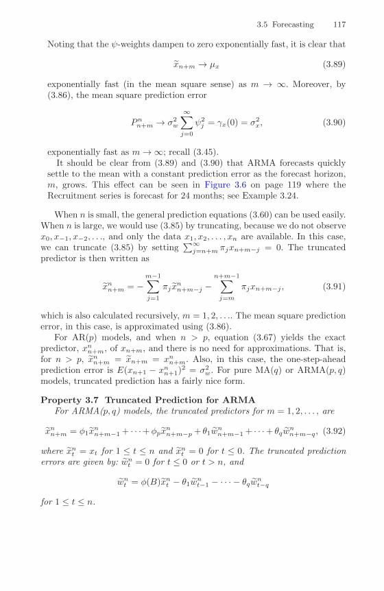
3.5 Forecasting 117
Noting that the ψ-weights dampen to zero exponentially fast, it is clear that
xn+m → µx (3.89)
exponentially fast (in the mean square sense) as m → ∞. Moreover, by(3.86), the mean square prediction error
Pnn+m → σ2w
∞∑j=0
ψ2j = γx(0) = σ2
x, (3.90)
exponentially fast as m→∞; recall (3.45).It should be clear from (3.89) and (3.90) that ARMA forecasts quickly
settle to the mean with a constant prediction error as the forecast horizon,m, grows. This effect can be seen in Figure 3.6 on page 119 where theRecruitment series is forecast for 24 months; see Example 3.24.
When n is small, the general prediction equations (3.60) can be used easily.When n is large, we would use (3.85) by truncating, because we do not observex0, x−1, x−2, . . ., and only the data x1, x2, . . . , xn are available. In this case,we can truncate (3.85) by setting
∑∞j=n+m πjxn+m−j = 0. The truncated
predictor is then written as
xnn+m = −m−1∑j=1
πj xnn+m−j −
n+m−1∑j=m
πjxn+m−j , (3.91)
which is also calculated recursively, m = 1, 2, . . .. The mean square predictionerror, in this case, is approximated using (3.86).
For AR(p) models, and when n > p, equation (3.67) yields the exactpredictor, xnn+m, of xn+m, and there is no need for approximations. That is,for n > p, xnn+m = xn+m = xnn+m. Also, in this case, the one-step-aheadprediction error is E(xn+1 − xnn+1)2 = σ2
w. For pure MA(q) or ARMA(p, q)models, truncated prediction has a fairly nice form.
Property 3.7 Truncated Prediction for ARMAFor ARMA(p, q) models, the truncated predictors for m = 1, 2, . . . , are
xnn+m = φ1xnn+m−1 + · · ·+φpx
nn+m−p + θ1w
nn+m−1 + · · ·+ θqw
nn+m−q, (3.92)
where xnt = xt for 1 ≤ t ≤ n and xnt = 0 for t ≤ 0. The truncated predictionerrors are given by: wnt = 0 for t ≤ 0 or t > n, and
wnt = φ(B)xnt − θ1wnt−1 − · · · − θqwnt−q
for 1 ≤ t ≤ n.

118 3 ARIMA Models
Example 3.23 Forecasting an ARMA(1, 1) Series
Given data x1, . . . , xn, for forecasting purposes, write the model as
xn+1 = φxn + wn+1 + θwn.
Then, based on (3.92), the one-step-ahead truncated forecast is
xnn+1 = φxn + 0 + θwnn.
For m ≥ 2, we havexnn+m = φxnn+m−1,
which can be calculated recursively, m = 2, 3, . . . .To calculate wnn, which is needed to initialize the successive forecasts, the
model can be written as wt = xt − φxt−1 − θwt−1 for t = 1, . . . , n. Fortruncated forecasting using (3.92), put wn0 = 0, x0 = 0, and then iterate theerrors forward in time
wnt = xt − φxt−1 − θwnt−1, t = 1, . . . , n.
The approximate forecast variance is computed from (3.86) using the ψ-weights determined as in Example 3.11. In particular, the ψ-weights satisfyψj = (φ+ θ)φj−1, for j ≥ 1. This result gives
Pnn+m = σ2w
[1 + (φ+ θ)2
m−1∑j=1
φ2(j−1)]
= σ2w
[1 +
(φ+ θ)2(1− φ2(m−1))(1− φ2)
].
To assess the precision of the forecasts, prediction intervals are typicallycalculated along with the forecasts. In general, (1−α) prediction intervals areof the form
xnn+m ± cα2√Pnn+m, (3.93)
where cα/2 is chosen to get the desired degree of confidence. For example,if the process is Gaussian, then choosing cα/2 = 2 will yield an approxi-mate 95% prediction interval for xn+m. If we are interested in establishingprediction intervals over more than one time period, then cα/2 should be ad-justed appropriately, for example, by using Bonferroni’s inequality [see (4.55)in Chapter 4 or Johnson and Wichern, 1992, Chapter 5].
Example 3.24 Forecasting the Recruitment Series
Using the parameter estimates as the actual parameter values, Figure 3.6shows the result of forecasting the Recruitment series given in Example 3.17over a 24-month horizon, m = 1, 2, . . . , 24. The actual forecasts are calcu-lated as
xnn+m = 6.74 + 1.35xnn+m−1 − .46xnn+m−2
for n = 453 and m = 1, 2, . . . , 12. Recall that xst = xt when t ≤ s. Theforecasts errors Pnn+m are calculated using (3.86). Recall that σ2
w = 89.72,
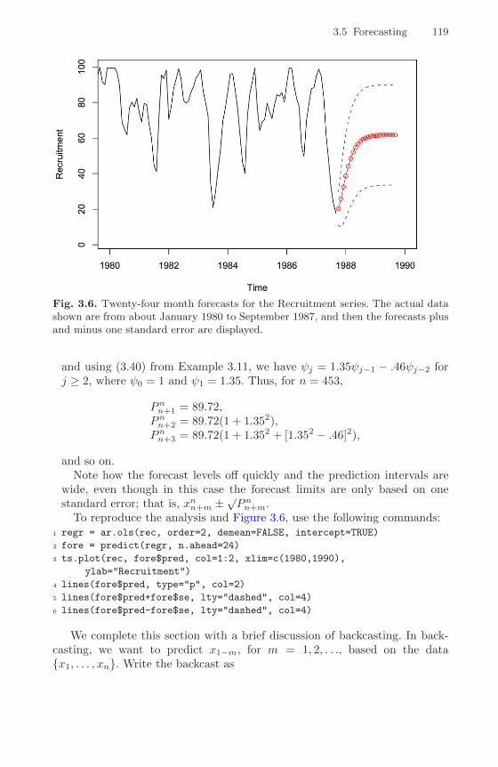
3.5 Forecasting 119
Fig. 3.6. Twenty-four month forecasts for the Recruitment series. The actual datashown are from about January 1980 to September 1987, and then the forecasts plusand minus one standard error are displayed.
and using (3.40) from Example 3.11, we have ψj = 1.35ψj−1 − .46ψj−2 forj ≥ 2, where ψ0 = 1 and ψ1 = 1.35. Thus, for n = 453,
Pnn+1 = 89.72,Pnn+2 = 89.72(1 + 1.352),Pnn+3 = 89.72(1 + 1.352 + [1.352 − .46]2),
and so on.Note how the forecast levels off quickly and the prediction intervals are
wide, even though in this case the forecast limits are only based on onestandard error; that is, xnn+m ±
√Pnn+m.
To reproduce the analysis and Figure 3.6, use the following commands:1 regr = ar.ols(rec, order=2, demean=FALSE, intercept=TRUE)
2 fore = predict(regr, n.ahead=24)
3 ts.plot(rec, fore$pred, col=1:2, xlim=c(1980,1990),
ylab="Recruitment")
4 lines(fore$pred, type="p", col=2)
5 lines(fore$pred+fore$se, lty="dashed", col=4)
6 lines(fore$pred-fore$se, lty="dashed", col=4)
We complete this section with a brief discussion of backcasting. In back-casting, we want to predict x1−m, for m = 1, 2, . . ., based on the data{x1, . . . , xn}. Write the backcast as

120 3 ARIMA Models
xn1−m =
n∑j=1
αjxj . (3.94)
Analogous to (3.74), the prediction equations (assuming µx = 0) are
n∑j=1
αjE(xjxk) = E(x1−mxk), k = 1, . . . , n, (3.95)
orn∑j=1
αjγ(k − j) = γ(m+ k − 1), k = 1, . . . , n. (3.96)
These equations are precisely the prediction equations for forward prediction.
That is, αj ≡ φ(m)nj , for j = 1, . . . , n, where the φ
(m)nj are given by (3.75).
Finally, the backcasts are given by
xn1−m = φ(m)n1 x1 + · · ·+ φ(m)
nn xn, m = 1, 2, . . . . (3.97)
Example 3.25 Backcasting an ARMA(1, 1)
Consider an ARMA(1, 1) process, xt = φxt−1 + θwt−1 +wt; we will call thisthe forward model. We have just seen that best linear prediction backwardin time is the same as best linear prediction forward in time for stationarymodels. Because we are assuming ARMA models are Gaussian, we also havethat minimum mean square error prediction backward in time is the sameas forward in time for ARMA models.4 Thus, the process can equivalentlybe generated by the backward model,
xt = φxt+1 + θvt+1 + vt,
where {vt} is a Gaussian white noise process with variance σ2w. We may
write xt =∑∞j=0 ψjvt+j , where ψ0 = 1; this means that xt is uncorrelated
with {vt−1, vt−2, . . .}, in analogy to the forward model.Given data {x1, . . . ., xn}, truncate vnn = E(vn |x1, . . . ., xn) to zero and
then iterate backward. That is, put vnn = 0, as an initial approximation, andthen generate the errors backward
vnt = xt − φxt+1 − θvnt+1, t = (n− 1), (n− 2), . . . , 1.
Then,xn0 = φx1 + θvn1 + vn0 = φx1 + θvn1 ,
because vnt = 0 for t ≤ 0. Continuing, the general truncated backcasts aregiven by
xn1−m = φxn2−m, m = 2, 3, . . . .
4 In the stationary Gaussian case, (a) the distribution of {xn+1, xn, . . . , x1} is thesame as (b) the distribution of {x0, x1 . . . , xn}. In forecasting we use (a) to ob-tain E(xn+1 |xn, . . . , x1); in backcasting we use (b) to obtain E(x0 |x1, . . . , xn).Because (a) and (b) are the same, the two problems are equivalent.
3.6 Estimation 121
3.6 Estimation
Throughout this section, we assume we have n observations, x1, . . . , xn, froma causal and invertible Gaussian ARMA(p, q) process in which, initially, theorder parameters, p and q, are known. Our goal is to estimate the parameters,φ1, . . . , φp, θ1, . . . , θq, and σ2
w. We will discuss the problem of determining pand q later in this section.
We begin with method of moments estimators. The idea behind these esti-mators is that of equating population moments to sample moments and thensolving for the parameters in terms of the sample moments. We immediatelysee that, if E(xt) = µ, then the method of moments estimator of µ is thesample average, x. Thus, while discussing method of moments, we will as-sume µ = 0. Although the method of moments can produce good estimators,they can sometimes lead to suboptimal estimators. We first consider the casein which the method leads to optimal (efficient) estimators, that is, AR(p)models.
When the process is AR(p),
xt = φ1xt−1 + · · ·+ φpxt−p + wt,
the first p+ 1 equations of (3.47) and (3.48) lead to the following:
Definition 3.10 The Yule–Walker equations are given by
γ(h) = φ1γ(h− 1) + · · ·+ φpγ(h− p), h = 1, 2, . . . , p, (3.98)
σ2w = γ(0)− φ1γ(1)− · · · − φpγ(p). (3.99)
In matrix notation, the Yule–Walker equations are
Γpφφφ = γγγp, σ2w = γ(0)− φφφ′γγγp, (3.100)
where Γp = {γ(k−j)}pj,k=1 is a p×p matrix, φφφ = (φ1, . . . , φp)′ is a p×1 vector,
and γγγp = (γ(1), . . . , γ(p))′
is a p × 1 vector. Using the method of moments,we replace γ(h) in (3.100) by γ(h) [see equation (1.34)] and solve
φφφ = Γ−1p γγγp, σ2w = γ(0)− γγγ′pΓ−1p γγγp. (3.101)
These estimators are typically called the Yule–Walker estimators. For calcula-tion purposes, it is sometimes more convenient to work with the sample ACF.By factoring γ(0) in (3.101), we can write the Yule–Walker estimates as
φφφ = RRR−1p ρρρp, σ2
w = γ(0)[1− ρρρ′pRRR
−1p ρρρp
], (3.102)
where Rp = {ρ(k − j)}pj,k=1 is a p × p matrix and ρρρp = (ρ(1), . . . , ρ(p))′
is ap× 1 vector.
For AR(p) models, if the sample size is large, the Yule–Walker estimatorsare approximately normally distributed, and σ2
w is close to the true value ofσ2w. We state these results in Property 3.8; for details, see Appendix B, §B.3.
122 3 ARIMA Models
Property 3.8 Large Sample Results for Yule–Walker EstimatorsThe asymptotic (n → ∞) behavior of the Yule–Walker estimators in the
case of causal AR(p) processes is as follows:
√n(φφφ− φφφ
)d→ N
(000, σ2
wΓ−1p
), σ2
wp→ σ2
w. (3.103)
The Durbin–Levinson algorithm, (3.68)-(3.70), can be used to calculate φφφ
without inverting Γp or Rp, by replacing γ(h) by γ(h) in the algorithm. In
running the algorithm, we will iteratively calculate the h × 1 vector, φφφh =
(φh1, . . . , φhh)′, for h = 1, 2, . . .. Thus, in addition to obtaining the desired
forecasts, the Durbin–Levinson algorithm yields φhh, the sample PACF. Using(3.103), we can show the following property.
Property 3.9 Large Sample Distribution of the PACFFor a causal AR(p) process, asymptotically (n→∞),
√n φhh
d→ N (0, 1) , for h > p. (3.104)
Example 3.26 Yule–Walker Estimation for an AR(2) Process
The data shown in Figure 3.3 were n = 144 simulated observations from theAR(2) model
xt = 1.5xt−1 − .75xt−2 + wt,
where wt ∼ iid N(0, 1). For these data, γ(0) = 8.903, ρ(1) = .849, andρ(2) = .519. Thus,
φφφ =
(φ1φ2
)=
[1 .849.849 1
]−1(.849.519
)=
(1.463−.723
)and
σ2w = 8.903
[1− (.849, .519)
(1.463−.723
)]= 1.187.
By Property 3.8, the asymptotic variance–covariance matrix of φφφ,
1
144
1.187
8.903
[1 .849.849 1
]−1=
[.0582 −.003−.003 .0582
],
can be used to get confidence regions for, or make inferences about φφφ andits components. For example, an approximate 95% confidence interval forφ2 is −.723 ± 2(.058), or (−.838,−.608), which contains the true value ofφ2 = −.75.
For these data, the first three sample partial autocorrelations are φ11 =ρ(1) = .849, φ22 = φ2 = −.721, and φ33 = −.085. According to Property 3.9,
the asymptotic standard error of φ33 is 1/√
144 = .083, and the observedvalue, −.085, is about only one standard deviation from φ33 = 0.

3.6 Estimation 123
Example 3.27 Yule–Walker Estimation of the Recruitment Series
In Example 3.17 we fit an AR(2) model to the recruitment series usingregression. Below are the results of fitting the same model using Yule-Walkerestimation in R, which are nearly identical to the values in Example 3.17.
1 rec.yw = ar.yw(rec, order=2)
2 rec.yw$x.mean # = 62.26 (mean estimate)
3 rec.yw$ar # = 1.33, -.44 (parameter estimates)
4 sqrt(diag(rec.yw$asy.var.coef)) # = .04, .04 (standard errors)
5 rec.yw$var.pred # = 94.80 (error variance estimate)
To obtain the 24 month ahead predictions and their standard errors, andthen plot the results as in Example 3.24, use the R commands:
1 rec.pr = predict(rec.yw, n.ahead=24)
2 U = rec.pr$pred + rec.pr$se
3 L = rec.pr$pred - rec.pr$se
4 minx = min(rec,L); maxx = max(rec,U)
5 ts.plot(rec, rec.pr$pred, xlim=c(1980,1990), ylim=c(minx,maxx))
6 lines(rec.pr$pred, col="red", type="o")
7 lines(U, col="blue", lty="dashed")
8 lines(L, col="blue", lty="dashed")
In the case of AR(p) models, the Yule–Walker estimators given in (3.102)are optimal in the sense that the asymptotic distribution, (3.103), is thebest asymptotic normal distribution. This is because, given initial conditions,AR(p) models are linear models, and the Yule–Walker estimators are essen-tially least squares estimators. If we use method of moments for MA or ARMAmodels, we will not get optimal estimators because such processes are nonlin-ear in the parameters.
Example 3.28 Method of Moments Estimation for an MA(1)
Consider the time seriesxt = wt + θwt−1,
where |θ| < 1. The model can then be written as
xt =∞∑j=1
(−θ)jxt−j + wt,
which is nonlinear in θ. The first two population autocovariances are γ(0) =σ2w(1 + θ2) and γ(1) = σ2
wθ, so the estimate of θ is found by solving:
ρ(1) =γ(1)
γ(0)=
θ
1 + θ2.
Two solutions exist, so we would pick the invertible one. If |ρ(1)| ≤ 12 , the
solutions are real, otherwise, a real solution does not exist. Even though|ρ(1)| < 1
2 for an invertible MA(1), it may happen that |ρ(1)| ≥ 12 because
it is an estimator. For example, the following simulation in R produces avalue of ρ(1) = .507 when the true value is ρ(1) = .9/(1 + .92) = .497.
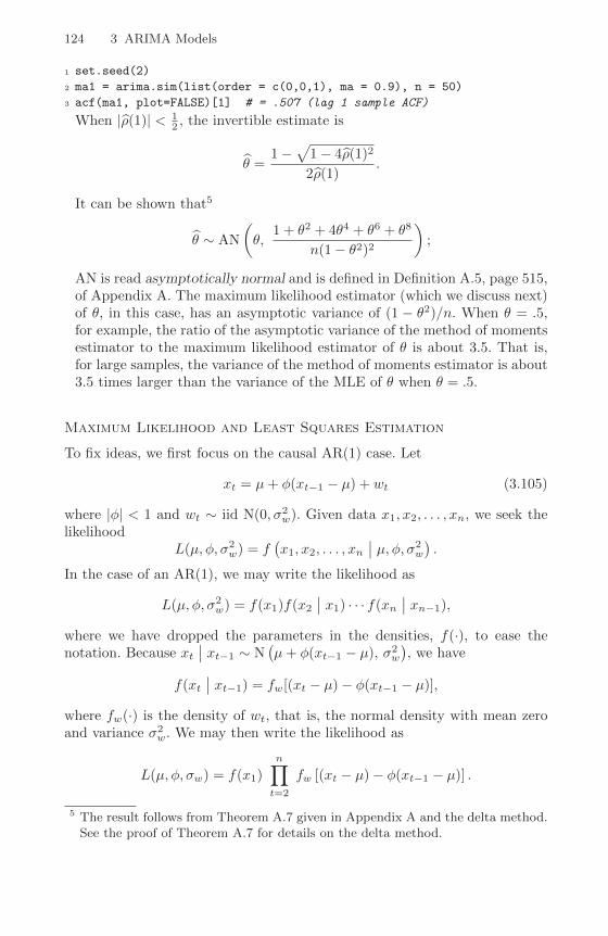
124 3 ARIMA Models
1 set.seed(2)
2 ma1 = arima.sim(list(order = c(0,0,1), ma = 0.9), n = 50)
3 acf(ma1, plot=FALSE)[1] # = .507 (lag 1 sample ACF)
When |ρ(1)| < 12 , the invertible estimate is
θ =1−
√1− 4ρ(1)2
2ρ(1).
It can be shown that5
θ ∼ AN
(θ,
1 + θ2 + 4θ4 + θ6 + θ8
n(1− θ2)2
);
AN is read asymptotically normal and is defined in Definition A.5, page 515,of Appendix A. The maximum likelihood estimator (which we discuss next)of θ, in this case, has an asymptotic variance of (1 − θ2)/n. When θ = .5,for example, the ratio of the asymptotic variance of the method of momentsestimator to the maximum likelihood estimator of θ is about 3.5. That is,for large samples, the variance of the method of moments estimator is about3.5 times larger than the variance of the MLE of θ when θ = .5.
Maximum Likelihood and Least Squares Estimation
To fix ideas, we first focus on the causal AR(1) case. Let
xt = µ+ φ(xt−1 − µ) + wt (3.105)
where |φ| < 1 and wt ∼ iid N(0, σ2w). Given data x1, x2, . . . , xn, we seek the
likelihoodL(µ, φ, σ2
w) = f(x1, x2, . . . , xn
∣∣ µ, φ, σ2w
).
In the case of an AR(1), we may write the likelihood as
L(µ, φ, σ2w) = f(x1)f(x2
∣∣ x1) · · · f(xn∣∣ xn−1),
where we have dropped the parameters in the densities, f(·), to ease thenotation. Because xt
∣∣ xt−1 ∼ N(µ+ φ(xt−1 − µ), σ2
w
), we have
f(xt∣∣ xt−1) = fw[(xt − µ)− φ(xt−1 − µ)],
where fw(·) is the density of wt, that is, the normal density with mean zeroand variance σ2
w. We may then write the likelihood as
L(µ, φ, σw) = f(x1)n∏t=2
fw [(xt − µ)− φ(xt−1 − µ)] .
5 The result follows from Theorem A.7 given in Appendix A and the delta method.See the proof of Theorem A.7 for details on the delta method.

3.6 Estimation 125
To find f(x1), we can use the causal representation
x1 = µ+∞∑j=0
φjw1−j
to see that x1 is normal, with mean µ and variance σ2w/(1− φ2). Finally, for
an AR(1), the likelihood is
L(µ, φ, σ2w) = (2πσ2
w)−n/2(1− φ2)1/2 exp
[−S(µ, φ)
2σ2w
], (3.106)
where
S(µ, φ) = (1− φ2)(x1 − µ)2 +n∑t=2
[(xt − µ)− φ(xt−1 − µ)]2. (3.107)
Typically, S(µ, φ) is called the unconditional sum of squares. We could havealso considered the estimation of µ and φ using unconditional least squares,that is, estimation by minimizing S(µ, φ).
Taking the partial derivative of the log of (3.106) with respect to σ2w and
setting the result equal to zero, we see that for any given values of µ and φin the parameter space, σ2
w = n−1S(µ, φ) maximizes the likelihood. Thus, themaximum likelihood estimate of σ2
w is
σ2w = n−1S(µ, φ), (3.108)
where µ and φ are the MLEs of µ and φ, respectively. If we replace n in (3.108)by n− 2, we would obtain the unconditional least squares estimate of σ2
w.If, in (3.106), we take logs, replace σ2
w by σ2w, and ignore constants, µ and
φ are the values that minimize the criterion function
l(µ, φ) = log[n−1S(µ, φ)
]− n−1 log(1− φ2); (3.109)
that is, l(µ, φ) ∝ −2 logL(µ, φ, σ2w).6 Because (3.107) and (3.109) are com-
plicated functions of the parameters, the minimization of l(µ, φ) or S(µ, φ) isaccomplished numerically. In the case of AR models, we have the advantagethat, conditional on initial values, they are linear models. That is, we candrop the term in the likelihood that causes the nonlinearity. Conditioning onx1, the conditional likelihood becomes
L(µ, φ, σ2w
∣∣ x1) =n∏t=2
fw [(xt − µ)− φ(xt−1 − µ)]
= (2πσ2w)−(n−1)/2 exp
[−Sc(µ, φ)
2σ2w
], (3.110)
6 The criterion function is sometimes called the profile or concentrated likelihood.

126 3 ARIMA Models
where the conditional sum of squares is
Sc(µ, φ) =n∑t=2
[(xt − µ)− φ(xt−1 − µ)]2. (3.111)
The conditional MLE of σ2w is
σ2w = Sc(µ, φ)/(n− 1), (3.112)
and µ and φ are the values that minimize the conditional sum of squares,Sc(µ, φ). Letting α = µ(1− φ), the conditional sum of squares can be writtenas
Sc(µ, φ) =n∑t=2
[xt − (α+ φxt−1)]2. (3.113)
The problem is now the linear regression problem stated in §2.2. Followingthe results from least squares estimation, we have α = x(2) − φx(1), where
x(1) = (n− 1)−1∑n−1t=1 xt, and x(2) = (n− 1)−1
∑nt=2 xt, and the conditional
estimates are then
µ =x(2) − φx(1)
1− φ(3.114)
φ =
∑nt=2(xt − x(2))(xt−1 − x(1))∑n
t=2(xt−1 − x(1))2. (3.115)
From (3.114) and (3.115), we see that µ ≈ x and φ ≈ ρ(1). That is, theYule–Walker estimators and the conditional least squares estimators are ap-proximately the same. The only difference is the inclusion or exclusion ofterms involving the endpoints, x1 and xn. We can also adjust the estimate ofσ2w in (3.112) to be equivalent to the least squares estimator, that is, divide
Sc(µ, φ) by (n− 3) instead of (n− 1) in (3.112).For general AR(p) models, maximum likelihood estimation, unconditional
least squares, and conditional least squares follow analogously to the AR(1)example. For general ARMA models, it is difficult to write the likelihood as anexplicit function of the parameters. Instead, it is advantageous to write thelikelihood in terms of the innovations, or one-step-ahead prediction errors,xt − xt−1t . This will also be useful in Chapter 6 when we study state-spacemodels.
For a normal ARMA(p, q) model, let βββ = (µ, φ1, . . . , φp, θ1, . . . , θq)′ be the
(p+ q+ 1)-dimensional vector of the model parameters. The likelihood can bewritten as
L(βββ, σ2w) =
n∏t=1
f(xt∣∣ xt−1, . . . , x1).
The conditional distribution of xt given xt−1, . . . , x1 is Gaussian with meanxt−1t and variance P t−1t . Recall from (3.71) that P t−1t = γ(0)
∏t−1j=1(1− φ2jj).
For ARMA models, γ(0) = σ2w
∑∞j=0 ψ
2j , in which case we may write

3.6 Estimation 127
P t−1t = σ2w
∞∑j=0
ψ2j
t−1∏j=1
(1− φ2jj)
def= σ2
w rt,
where rt is the term in the braces. Note that the rt terms are functions onlyof the regression parameters and that they may be computed recursively asrt+1 = (1− φ2tt)rt with initial condition r1 =
∑∞j=0 ψ
2j . The likelihood of the
data can now be written as
L(βββ, σ2w) = (2πσ2
w)−n/2 [r1(βββ)r2(βββ) · · · rn(βββ)]−1/2
exp
[−S(βββ)
2σ2w
], (3.116)
where
S(βββ) =n∑t=1
[(xt − xt−1t (βββ))2
rt(βββ)
]. (3.117)
Both xt−1t and rt are functions of βββ alone, and we make that fact explicitin (3.116)-(3.117). Given values for βββ and σ2
w, the likelihood may be evalu-ated using the techniques of §3.5. Maximum likelihood estimation would nowproceed by maximizing (3.116) with respect to βββ and σ2
w. As in the AR(1)example, we have
σ2w = n−1S(βββ), (3.118)
where βββ is the value of βββ that minimizes the concentrated likelihood
l(βββ) = log[n−1S(βββ)
]+ n−1
n∑t=1
log rt(βββ). (3.119)
For the AR(1) model (3.105) discussed previously, recall that x01 = µ andxt−1t = µ + φ(xt−1 − µ), for t = 2, . . . , n. Also, using the fact that φ11 = φand φhh = 0 for h > 1, we have r1 =
∑∞j=0 φ
2j = (1 − φ2)−1, r2 = (1 −φ2)−1(1−φ2) = 1, and in general, rt = 1 for t = 2, . . . , n. Hence, the likelihoodpresented in (3.106) is identical to the innovations form of the likelihood givenby (3.116). Moreover, the generic S(βββ) in (3.117) is S(µ, φ) given in (3.107)and the generic l(βββ) in (3.119) is l(µ, φ) in (3.109).
Unconditional least squares would be performed by minimizing (3.117)with respect to βββ. Conditional least squares estimation would involve mini-mizing (3.117) with respect to βββ but where, to ease the computational burden,the predictions and their errors are obtained by conditioning on initial valuesof the data. In general, numerical optimization routines are used to obtain theactual estimates and their standard errors.
Example 3.29 The Newton–Raphson and Scoring Algorithms
Two common numerical optimization routines for accomplishing maximumlikelihood estimation are Newton–Raphson and scoring. We will give a briefaccount of the mathematical ideas here. The actual implementation of thesealgorithms is much more complicated than our discussion might imply. For
128 3 ARIMA Models
details, the reader is referred to any of the Numerical Recipes books, forexample, Press et al. (1993).
Let l(βββ) be a criterion function of k parameters βββ = (β1, . . . , βk) that wewish to minimize with respect to βββ. For example, consider the likelihoodfunction given by (3.109) or by (3.119). Suppose l(βββ) is the extremum that
we are interested in finding, and βββ is found by solving ∂l(βββ)/∂βj = 0, forj = 1, . . . , k. Let l(1)(βββ) denote the k × 1 vector of partials
l(1)(βββ) =
(∂l(βββ)
∂β1, . . . ,
∂l(βββ)
∂βk
)′.
Note, l(1)(βββ) = 000, the k× 1 zero vector. Let l(2)(βββ) denote the k× k matrixof second-order partials
l(2)(βββ) =
{− ∂l
2(βββ)
∂βi∂βj
}ki,j=1
,
and assume l(2)(βββ) is nonsingular. Let βββ(0) be an initial estimator of βββ. Then,using a Taylor expansion, we have the following approximation:
000 = l(1)(βββ) ≈ l(1)(βββ(0))− l(2)(βββ(0))[βββ − βββ(0)
].
Setting the right-hand side equal to zero and solving for βββ [call the solutionβββ(1)], we get
βββ(1) = βββ(0) +[l(2)(βββ(0))
]−1l(1)(βββ(0)).
The Newton–Raphson algorithm proceeds by iterating this result, replacingβββ(0) by βββ(1) to get βββ(2), and so on, until convergence. Under a set of appro-priate conditions, the sequence of estimators, βββ(1), βββ(2), . . ., will converge to
βββ, the MLE of βββ.For maximum likelihood estimation, the criterion function used is l(βββ)
given by (3.119); l(1)(βββ) is called the score vector, and l(2)(βββ) is called theHessian. In the method of scoring, we replace l(2)(βββ) by E[l(2)(βββ)], the in-formation matrix. Under appropriate conditions, the inverse of the informa-tion matrix is the asymptotic variance–covariance matrix of the estimatorβββ. This is sometimes approximated by the inverse of the Hessian at βββ. Ifthe derivatives are difficult to obtain, it is possible to use quasi-maximumlikelihood estimation where numerical techniques are used to approximatethe derivatives.
Example 3.30 MLE for the Recruitment Series
So far, we have fit an AR(2) model to the Recruitment series using ordinaryleast squares (Example 3.17) and using Yule–Walker (Example 3.27). Thefollowing is an R session used to fit an AR(2) model via maximum likelihoodestimation to the Recruitment series; these results can be compared to theresults in Examples 3.17 and 3.27.
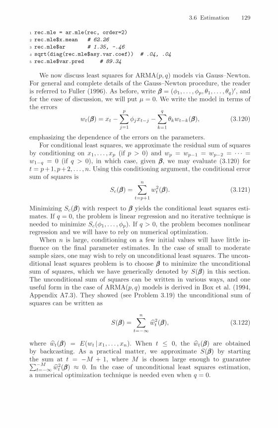
3.6 Estimation 129
1 rec.mle = ar.mle(rec, order=2)
2 rec.mle$x.mean # 62.26
3 rec.mle$ar # 1.35, -.46
4 sqrt(diag(rec.mle$asy.var.coef)) # .04, .04
5 rec.mle$var.pred # 89.34
We now discuss least squares for ARMA(p, q) models via Gauss–Newton.For general and complete details of the Gauss–Newton procedure, the readeris referred to Fuller (1996). As before, write βββ = (φ1, . . . , φp, θ1, . . . , θq)
′, andfor the ease of discussion, we will put µ = 0. We write the model in terms ofthe errors
wt(βββ) = xt −p∑j=1
φjxt−j −q∑
k=1
θkwt−k(βββ), (3.120)
emphasizing the dependence of the errors on the parameters.For conditional least squares, we approximate the residual sum of squares
by conditioning on x1, . . . , xp (if p > 0) and wp = wp−1 = wp−2 = · · · =w1−q = 0 (if q > 0), in which case, given βββ, we may evaluate (3.120) fort = p+1, p+2, . . . , n. Using this conditioning argument, the conditional errorsum of squares is
Sc(βββ) =
n∑t=p+1
w2t (βββ). (3.121)
Minimizing Sc(βββ) with respect to βββ yields the conditional least squares esti-mates. If q = 0, the problem is linear regression and no iterative technique isneeded to minimize Sc(φ1, . . . , φp). If q > 0, the problem becomes nonlinearregression and we will have to rely on numerical optimization.
When n is large, conditioning on a few initial values will have little in-fluence on the final parameter estimates. In the case of small to moderatesample sizes, one may wish to rely on unconditional least squares. The uncon-ditional least squares problem is to choose βββ to minimize the unconditionalsum of squares, which we have generically denoted by S(βββ) in this section.The unconditional sum of squares can be written in various ways, and oneuseful form in the case of ARMA(p, q) models is derived in Box et al. (1994,Appendix A7.3). They showed (see Problem 3.19) the unconditional sum ofsquares can be written as
S(βββ) =
n∑t=−∞
w2t (βββ), (3.122)
where wt(βββ) = E(wt |x1, . . . , xn). When t ≤ 0, the wt(βββ) are obtainedby backcasting. As a practical matter, we approximate S(βββ) by startingthe sum at t = −M + 1, where M is chosen large enough to guarantee∑−Mt=−∞ w2
t (βββ) ≈ 0. In the case of unconditional least squares estimation,a numerical optimization technique is needed even when q = 0.

130 3 ARIMA Models
To employ Gauss–Newton, let βββ(0) = (φ(0)1 , . . . , φ
(0)p , θ
(0)1 , . . . , θ
(0)q )′ be an
initial estimate of βββ. For example, we could obtain βββ(0) by method of moments.The first-order Taylor expansion of wt(βββ) is
wt(βββ) ≈ wt(βββ(0))−(βββ − βββ(0)
)′zzzt(βββ(0)), (3.123)
where
zzzt(βββ(0)) =
(−∂wt(βββ(0))
∂β1, . . . ,−
∂wt(βββ(0))
∂βp+q
)′, t = 1, . . . , n.
The linear approximation of Sc(βββ) is
Q(βββ) =n∑
t=p+1
[wt(βββ(0))−
(βββ − βββ(0)
)′zzzt(βββ(0))
]2(3.124)
and this is the quantity that we will minimize. For approximate unconditionalleast squares, we would start the sum in (3.124) at t = −M + 1, for a largevalue of M , and work with the backcasted values.
Using the results of ordinary least squares (§2.2), we know
(βββ − βββ(0)) =(n−1
n∑t=p+1
zzzt(βββ(0))zzz′t(βββ(0))
)−1(n−1
n∑t=p+1
zzzt(βββ(0))wt(βββ(0)))
(3.125)minimizes Q(βββ). From (3.125), we write the one-step Gauss–Newton estimateas
βββ(1) = βββ(0) +∆(βββ(0)), (3.126)
where ∆(βββ(0)) denotes the right-hand side of (3.125). Gauss–Newton esti-mation is accomplished by replacing βββ(0) by βββ(1) in (3.126). This process isrepeated by calculating, at iteration j = 2, 3, . . .,
βββ(j) = βββ(j−1) +∆(βββ(j−1))
until convergence.
Example 3.31 Gauss–Newton for an MA(1)
Consider an invertible MA(1) process, xt = wt+θwt−1. Write the truncatederrors as
wt(θ) = xt − θwt−1(θ), t = 1, . . . , n, (3.127)
where we condition on w0(θ) = 0. Taking derivatives,
−∂wt(θ)∂θ
= wt−1(θ) + θ∂wt−1(θ)
∂θ, t = 1, . . . , n, (3.128)
where ∂w0(θ)/∂θ = 0. Using the notation of (3.123), we can also write(3.128) as

3.6 Estimation 131
0 5 10 15 20 25 30 35
−0.4
0.0
0.4
0.8
LAG
ACF
0 5 10 15 20 25 30 35
−0.4
0.0
0.4
0.8
LAG
PACF
Fig. 3.7. ACF and PACF of transformed glacial varves.
zt(θ) = wt−1(θ)− θzt−1(θ), t = 1, . . . , n, (3.129)
where z0(θ) = 0.Let θ(0) be an initial estimate of θ, for example, the estimate given in Ex-
ample 3.28. Then, the Gauss–Newton procedure for conditional least squaresis given by
θ(j+1) = θ(j) +
∑nt=1 zt(θ(j))wt(θ(j))∑n
t=1 z2t (θ(j))
, j = 0, 1, 2, . . . , (3.130)
where the values in (3.130) are calculated recursively using (3.127) and(3.129). The calculations are stopped when |θ(j+1) − θ(j)|, or |Q(θ(j+1)) −Q(θ(j))|, are smaller than some preset amount.
Example 3.32 Fitting the Glacial Varve Series
Consider the series of glacial varve thicknesses from Massachusetts for n =634 years, as analyzed in Example 2.6 and in Problem 2.8, where it wasargued that a first-order moving average model might fit the logarithmicallytransformed and differenced varve series, say,
∇ log(xt) = log(xt)− log(xt−1) = log
(xtxt−1
),
which can be interpreted as being approximately the percentage change inthe thickness.
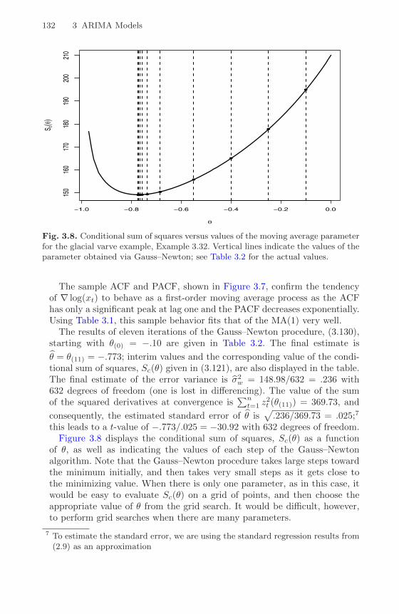
132 3 ARIMA Models
−1.0 −0.8 −0.6 −0.4 −0.2 0.0
150
160
170
180
190
200
210
S c
Fig. 3.8. Conditional sum of squares versus values of the moving average parameterfor the glacial varve example, Example 3.32. Vertical lines indicate the values of theparameter obtained via Gauss–Newton; see Table 3.2 for the actual values.
The sample ACF and PACF, shown in Figure 3.7, confirm the tendencyof ∇ log(xt) to behave as a first-order moving average process as the ACFhas only a significant peak at lag one and the PACF decreases exponentially.Using Table 3.1, this sample behavior fits that of the MA(1) very well.
The results of eleven iterations of the Gauss–Newton procedure, (3.130),starting with θ(0) = −.10 are given in Table 3.2. The final estimate is
θ = θ(11) = −.773; interim values and the corresponding value of the condi-tional sum of squares, Sc(θ) given in (3.121), are also displayed in the table.The final estimate of the error variance is σ2
w = 148.98/632 = .236 with632 degrees of freedom (one is lost in differencing). The value of the sumof the squared derivatives at convergence is
∑nt=1 z
2t (θ(11)) = 369.73, and
consequently, the estimated standard error of θ is√.236/369.73 = .025;7
this leads to a t-value of −.773/.025 = −30.92 with 632 degrees of freedom.Figure 3.8 displays the conditional sum of squares, Sc(θ) as a function
of θ, as well as indicating the values of each step of the Gauss–Newtonalgorithm. Note that the Gauss–Newton procedure takes large steps towardthe minimum initially, and then takes very small steps as it gets close tothe minimizing value. When there is only one parameter, as in this case, itwould be easy to evaluate Sc(θ) on a grid of points, and then choose theappropriate value of θ from the grid search. It would be difficult, however,to perform grid searches when there are many parameters.
7 To estimate the standard error, we are using the standard regression results from(2.9) as an approximation

3.6 Estimation 133
Table 3.2. Gauss–Newton Results for Example 3.32
j θ(j) Sc(θ(j))∑nt=1 z
2t (θ(j))
0 −0.100 195.0010 183.34641 −0.250 177.7614 163.30382 −0.400 165.0027 161.62793 −0.550 155.6723 182.64324 −0.684 150.2896 247.49425 −0.736 149.2283 304.31256 −0.757 149.0272 337.92007 −0.766 148.9885 355.04658 −0.770 148.9812 363.28139 −0.771 148.9804 365.404510 −0.772 148.9799 367.554411 −0.773 148.9799 369.7314
In the general case of causal and invertible ARMA(p, q) models, maxi-mum likelihood estimation and conditional and unconditional least squaresestimation (and Yule–Walker estimation in the case of AR models) all lead tooptimal estimators. The proof of this general result can be found in a num-ber of texts on theoretical time series analysis (for example, Brockwell andDavis, 1991, or Hannan, 1970, to mention a few). We will denote the ARMAcoefficient parameters by βββ = (φ1, . . . , φp, θ1, . . . , θq)
′.
Property 3.10 Large Sample Distribution of the EstimatorsUnder appropriate conditions, for causal and invertible ARMA processes,
the maximum likelihood, the unconditional least squares, and the conditionalleast squares estimators, each initialized by the method of moments estimator,all provide optimal estimators of σ2
w and βββ, in the sense that σ2w is consistent,
and the asymptotic distribution of βββ is the best asymptotic normal distribution.In particular, as n→∞,
√n(βββ − βββ
)d→ N
(000, σ2
w ΓΓΓ−1p,q). (3.131)
The asymptotic variance–covariance matrix of the estimator βββ is the inverseof the information matrix. In particular, the (p+ q)× (p+ q) matrix Γp,q, hasthe form
Γp,q =
(Γφφ ΓφθΓθφ Γθθ
). (3.132)
The p×p matrix Γφφ is given by (3.100), that is, the ij-th element of Γφφ, fori, j = 1, . . . , p, is γx(i−j) from an AR(p) process, φ(B)xt = wt. Similarly, Γθθis a q × q matrix with the ij-th element, for i, j = 1, . . . , q, equal to γy(i− j)from an AR(q) process, θ(B)yt = wt. The p × q matrix Γφθ = {γxy(i − j)},for i = 1, . . . , p; j = 1, . . . , q; that is, the ij-th element is the cross-covariance
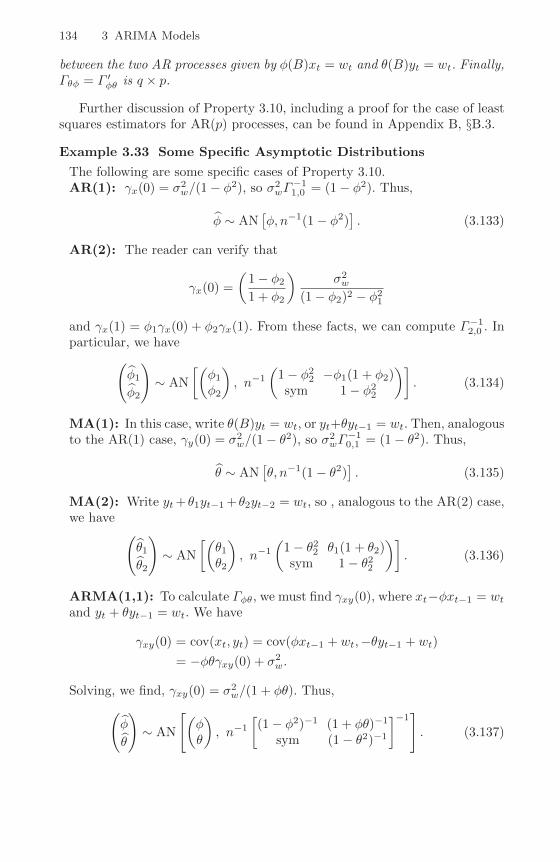
134 3 ARIMA Models
between the two AR processes given by φ(B)xt = wt and θ(B)yt = wt. Finally,Γθφ = Γ ′φθ is q × p.
Further discussion of Property 3.10, including a proof for the case of leastsquares estimators for AR(p) processes, can be found in Appendix B, §B.3.
Example 3.33 Some Specific Asymptotic Distributions
The following are some specific cases of Property 3.10.AR(1): γx(0) = σ2
w/(1− φ2), so σ2wΓ−11,0 = (1− φ2). Thus,
φ ∼ AN[φ, n−1(1− φ2)
]. (3.133)
AR(2): The reader can verify that
γx(0) =
(1− φ21 + φ2
)σ2w
(1− φ2)2 − φ21
and γx(1) = φ1γx(0) + φ2γx(1). From these facts, we can compute Γ−12,0 . Inparticular, we have(
φ1φ2
)∼ AN
[(φ1φ2
), n−1
(1− φ22 −φ1(1 + φ2)sym 1− φ22
)]. (3.134)
MA(1): In this case, write θ(B)yt = wt, or yt+θyt−1 = wt. Then, analogousto the AR(1) case, γy(0) = σ2
w/(1− θ2), so σ2wΓ−10,1 = (1− θ2). Thus,
θ ∼ AN[θ, n−1(1− θ2)
]. (3.135)
MA(2): Write yt+θ1yt−1 +θ2yt−2 = wt, so , analogous to the AR(2) case,we have (
θ1θ2
)∼ AN
[(θ1θ2
), n−1
(1− θ22 θ1(1 + θ2)sym 1− θ22
)]. (3.136)
ARMA(1,1): To calculate Γφθ, we must find γxy(0), where xt−φxt−1 = wtand yt + θyt−1 = wt. We have
γxy(0) = cov(xt, yt) = cov(φxt−1 + wt,−θyt−1 + wt)
= −φθγxy(0) + σ2w.
Solving, we find, γxy(0) = σ2w/(1 + φθ). Thus,(
φ
θ
)∼ AN
[(φθ
), n−1
[(1− φ2)−1 (1 + φθ)−1
sym (1− θ2)−1
]−1]. (3.137)

3.6 Estimation 135
Example 3.34 Overfitting Caveat
The asymptotic behavior of the parameter estimators gives us an additionalinsight into the problem of fitting ARMA models to data. For example,suppose a time series follows an AR(1) process and we decide to fit anAR(2) to the data. Do any problems occur in doing this? More generally,why not simply fit large-order AR models to make sure that we capturethe dynamics of the process? After all, if the process is truly an AR(1), theother autoregressive parameters will not be significant. The answer is thatif we overfit, we obtain less efficient, or less precise parameter estimates.For example, if we fit an AR(1) to an AR(1) process, for large n, var(φ1) ≈n−1(1 − φ21). But, if we fit an AR(2) to the AR(1) process, for large n,
var(φ1) ≈ n−1(1− φ22) = n−1 because φ2 = 0. Thus, the variance of φ1 hasbeen inflated, making the estimator less precise.
We do want to mention, however, that overfitting can be used as a di-agnostic tool. For example, if we fit an AR(2) model to the data and aresatisfied with that model, then adding one more parameter and fitting anAR(3) should lead to approximately the same model as in the AR(2) fit. Wewill discuss model diagnostics in more detail in §3.8.
The reader might wonder, for example, why the asymptotic distributionsof φ from an AR(1) and θ from an MA(1) are of the same form; compare(3.133) to (3.135). It is possible to explain this unexpected result heuristicallyusing the intuition of linear regression. That is, for the normal regressionmodel presented in §2.2 with no intercept term, xt = βzt + wt, we know β isnormally distributed with mean β, and from (2.9),
var{√
n(β − β
)}= nσ2
w
(n∑t=1
z2t
)−1= σ2
w
(n−1
n∑t=1
z2t
)−1.
For the causal AR(1) model given by xt = φxt−1 + wt, the intuition ofregression tells us to expect that, for n large,
√n(φ− φ
)is approximately normal with mean zero and with variance given by
σ2w
(n−1
n∑t=2
x2t−1
)−1.
Now, n−1∑nt=2 x
2t−1 is the sample variance (recall that the mean of xt is zero)
of the xt, so as n becomes large we would expect it to approach var(xt) =
γ(0) = σ2w/(1− φ2). Thus, the large sample variance of
√n(φ− φ
)is
σ2wγx(0)−1 = σ2
w
(σ2w
1− φ2
)−1= (1− φ2);

136 3 ARIMA Models
that is, (3.133) holds.In the case of an MA(1), we may use the discussion of Example 3.31 to
write an approximate regression model for the MA(1). That is, consider theapproximation (3.129) as the regression model
zt(θ) = −θzt−1(θ) + wt−1,
where now, zt−1(θ) as defined in Example 3.31, plays the role of the regressor.Continuing with the analogy, we would expect the asymptotic distribution of√n(θ − θ
)to be normal, with mean zero, and approximate variance
σ2w
(n−1
n∑t=2
z2t−1(θ)
)−1.
As in the AR(1) case, n−1∑nt=2 z
2t−1(θ) is the sample variance of the zt(θ)
so, for large n, this should be var{zt(θ)} = γz(0), say. But note, as seen from(3.129), zt(θ) is approximately an AR(1) process with parameter −θ. Thus,
σ2wγz(0)−1 = σ2
w
(σ2w
1− (−θ)2
)−1= (1− θ2),
which agrees with (3.135). Finally, the asymptotic distributions of the ARparameter estimates and the MA parameter estimates are of the same formbecause in the MA case, the “regressors” are the differential processes zt(θ)that have AR structure, and it is this structure that determines the asymptoticvariance of the estimators. For a rigorous account of this approach for thegeneral case, see Fuller (1996, Theorem 5.5.4).
In Example 3.32, the estimated standard error of θ was .025. In that ex-ample, we used regression results to estimate the standard error as the squareroot of
n−1σ2w
(n−1
n∑t=1
z2t (θ)
)−1=
σ2w∑n
t=1 z2t (θ)
,
where n = 632, σ2w = .236,
∑nt=1 z
2t (θ) = 369.73 and θ = −.773. Using (3.135),
we could have also calculated this value using the asymptotic approximation,the square root of (1− (−.773)2)/632, which is also .025.
If n is small, or if the parameters are close to the boundaries, the asymp-totic approximations can be quite poor. The bootstrap can be helpful in thiscase; for a broad treatment of the bootstrap, see Efron and Tibshirani (1994).We discuss the case of an AR(1) here and leave the general discussion forChapter 6. For now, we give a simple example of the bootstrap for an AR(1)process.
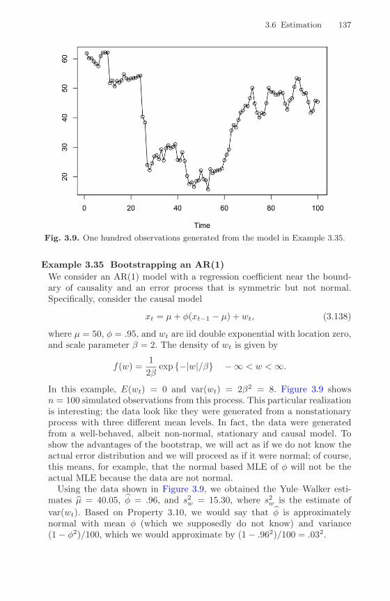
3.6 Estimation 137
Fig. 3.9. One hundred observations generated from the model in Example 3.35.
Example 3.35 Bootstrapping an AR(1)
We consider an AR(1) model with a regression coefficient near the bound-ary of causality and an error process that is symmetric but not normal.Specifically, consider the causal model
xt = µ+ φ(xt−1 − µ) + wt, (3.138)
where µ = 50, φ = .95, and wt are iid double exponential with location zero,and scale parameter β = 2. The density of wt is given by
f(w) =1
2βexp {−|w|/β} −∞ < w <∞.
In this example, E(wt) = 0 and var(wt) = 2β2 = 8. Figure 3.9 showsn = 100 simulated observations from this process. This particular realizationis interesting; the data look like they were generated from a nonstationaryprocess with three different mean levels. In fact, the data were generatedfrom a well-behaved, albeit non-normal, stationary and causal model. Toshow the advantages of the bootstrap, we will act as if we do not know theactual error distribution and we will proceed as if it were normal; of course,this means, for example, that the normal based MLE of φ will not be theactual MLE because the data are not normal.
Using the data shown in Figure 3.9, we obtained the Yule–Walker esti-mates µ = 40.05, φ = .96, and s2w = 15.30, where s2w is the estimate of
var(wt). Based on Property 3.10, we would say that φ is approximatelynormal with mean φ (which we supposedly do not know) and variance(1− φ2)/100, which we would approximate by (1− .962)/100 = .032.
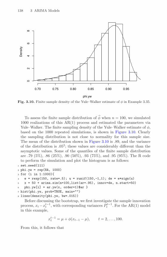
138 3 ARIMA Models
phi.yw
Den
sity
0.70 0.75 0.80 0.85 0.90 0.95
02
46
8
Fig. 3.10. Finite sample density of the Yule–Walker estimate of φ in Example 3.35.
To assess the finite sample distribution of φ when n = 100, we simulated1000 realizations of this AR(1) process and estimated the parameters viaYule–Walker. The finite sampling density of the Yule–Walker estimate of φ,based on the 1000 repeated simulations, is shown in Figure 3.10. Clearlythe sampling distribution is not close to normality for this sample size.The mean of the distribution shown in Figure 3.10 is .89, and the varianceof the distribution is .052; these values are considerably different than theasymptotic values. Some of the quantiles of the finite sample distributionare .79 (5%), .86 (25%), .90 (50%), .93 (75%), and .95 (95%). The R codeto perform the simulation and plot the histogram is as follows:
1 set.seed(111)
2 phi.yw = rep(NA, 1000)
3 for (i in 1:1000){
4 e = rexp(150, rate=.5); u = runif(150,-1,1); de = e*sign(u)
5 x = 50 + arima.sim(n=100,list(ar=.95), innov=de, n.start=50)
6 phi.yw[i] = ar.yw(x, order=1)$ar }
7 hist(phi.yw, prob=TRUE, main="")
8 lines(density(phi.yw, bw=.015))
Before discussing the bootstrap, we first investigate the sample innovationprocess, xt−xt−1t , with corresponding variances P t−1t . For the AR(1) modelin this example,
xt−1t = µ+ φ(xt−1 − µ), t = 2, . . . , 100.
From this, it follows that

3.6 Estimation 139
P t−1t = E(xt − xt−1t )2 = σ2w, t = 2, . . . , 100.
When t = 1, we have
x01 = µ and P 01 = σ2
w/(1− φ2).
Thus, the innovations have zero mean but different variances; in order thatall of the innovations have the same variance, σ2
w, we will write them as
ε1 = (x1 − µ)√
(1− φ2)
εt = (xt − µ)− φ(xt−1 − µ), for t = 2, . . . , 100. (3.139)
From these equations, we can write the model in terms of the εt as
x1 = µ+ ε1/√
(1− φ2)
xt = µ+ φ(xt−1 − µ) + εt for t = 2, . . . , 100. (3.140)
Next, replace the parameters with their estimates in (3.139), that is,
µ = 40.048 and φ = .957, and denote the resulting sample innovationsas {ε1, . . . , ε100}. To obtain one bootstrap sample, first randomly sample,with replacement, n = 100 values from the set of sample innovations; callthe sampled values {ε∗1, . . . , ε∗100}. Now, generate a bootstrapped data setsequentially by setting
x∗1 = 40.048 + ε∗1/√
(1− .9572)
x∗t = 40.048 + .957(x∗t−1 − 40.048) + ε∗t , t = 2, . . . , n. (3.141)
Next, estimate the parameters as if the data were x∗t . Call these esti-
mates µ(1), φ(1), and s2w(1). Repeat this process a large number, B,of times, generating a collection of bootstrapped parameter estimates,{µ(b), φ(b), s2w(b), b = 1, . . . , B}. We can then approximate the finite sampledistribution of an estimator from the bootstrapped parameter values. Forexample, we can approximate the distribution of φ − φ by the empiricaldistribution of φ(b)− φ, for b = 1, . . . , B.
Figure 3.11 shows the bootstrap histogram of 200 bootstrapped estimatesof φ using the data shown in Figure 3.9. In addition, Figure 3.11 shows adensity estimate based on the bootstrap histogram, as well as the asymp-totic normal density that would have been used based on Proposition 3.10.Clearly, the bootstrap distribution of φ is closer to the distribution of φshown in Figure 3.10 than to the asymptotic normal approximation. In par-ticular, the mean of the distribution of φ(b) is .92 with a variance of .052.Some quantiles of this distribution are .83 (5%), .90 (25%), .93 (50%), .95(75%), and .98 (95%).
To perform a similar bootstrap exercise in R, use the following commands.We note that the R estimation procedure is conditional on the first obser-vation, so the first residual is not returned. To get around this problem,

140 3 ARIMA Models
phi.star.yw
Den
sity
0.75 0.80 0.85 0.90 0.95 1.00 1.05
02
46
810
1214
Fig. 3.11. Bootstrap histogram of φ based on 200 bootstraps; a density estimatebased on the histogram (solid line) and the corresponding asymptotic normal density(dashed line).
we simply fix the first observation and bootstrap the remaining data. Thesimulated data are available in the file ar1boot, but you can simulate yourown data as was done in the code that produced Figure 3.10.
1 x = ar1boot
2 m = mean(x) # estimate of mu
3 fit = ar.yw(x, order=1)
4 phi = fit$ar # estimate of phi
5 nboot = 200 # number of bootstrap replicates
6 resids = fit$resid[-1] # the first resid is NA
7 x.star = x # initialize x*
8 phi.star.yw = rep(NA, nboot)
9 for (i in 1:nboot) {
10 resid.star = sample(resids, replace=TRUE)
11 for (t in 1:99){ x.star[t+1] = m + phi*(x.star[t]-m) +
resid.star[t] }
12 phi.star.yw[i] = ar.yw(x.star, order=1)$ar }
13 hist(phi.star.yw, 10, main="", prob=TRUE, ylim=c(0,14),
xlim=c(.75,1.05))
14 lines(density(phi.star.yw, bw=.02))
15 u = seq(.75, 1.05, by=.001)
16 lines(u, dnorm(u, mean=.96, sd=.03), lty="dashed", lwd=2)

3.7 Integrated Models for Nonstationary Data 141
3.7 Integrated Models for Nonstationary Data
In Chapters 1 and 2, we saw that if xt is a random walk, xt = xt−1 + wt,then by differencing xt, we find that ∇xt = wt is stationary. In many situa-tions, time series can be thought of as being composed of two components, anonstationary trend component and a zero-mean stationary component. Forexample, in §2.2 we considered the model
xt = µt + yt, (3.142)
where µt = β0 +β1t and yt is stationary. Differencing such a process will leadto a stationary process:
∇xt = xt − xt−1 = β1 + yt − yt−1 = β1 +∇yt.
Another model that leads to first differencing is the case in which µt in (3.142)is stochastic and slowly varying according to a random walk. That is,
µt = µt−1 + vt
where vt is stationary. In this case,
∇xt = vt +∇yt,
is stationary. If µt in (3.142) is a k-th order polynomial, µt =∑kj=0 βjt
j ,
then (Problem 3.27) the differenced series ∇kyt is stationary. Stochastic trendmodels can also lead to higher order differencing. For example, suppose
µt = µt−1 + vt and vt = vt−1 + et,
where et is stationary. Then, ∇xt = vt +∇yt is not stationary, but
∇2xt = et +∇2yt
is stationary.The integrated ARMA, or ARIMA, model is a broadening of the class of
ARMA models to include differencing.
Definition 3.11 A process xt is said to be ARIMA(p, d, q) if
∇dxt = (1−B)dxt
is ARMA(p, q). In general, we will write the model as
φ(B)(1−B)dxt = θ(B)wt. (3.143)
If E(∇dxt) = µ, we write the model as
φ(B)(1−B)dxt = δ + θ(B)wt,
where δ = µ(1− φ1 − · · · − φp).
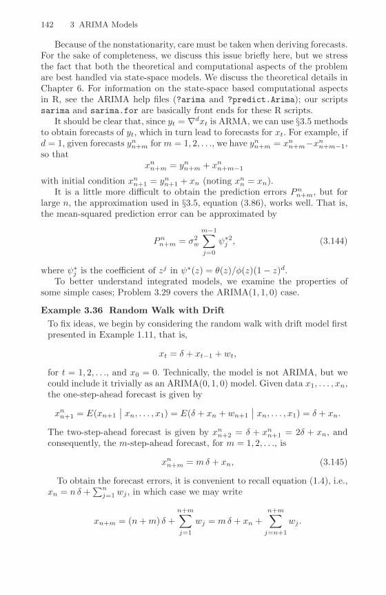
142 3 ARIMA Models
Because of the nonstationarity, care must be taken when deriving forecasts.For the sake of completeness, we discuss this issue briefly here, but we stressthe fact that both the theoretical and computational aspects of the problemare best handled via state-space models. We discuss the theoretical details inChapter 6. For information on the state-space based computational aspectsin R, see the ARIMA help files (?arima and ?predict.Arima); our scriptssarima and sarima.for are basically front ends for these R scripts.
It should be clear that, since yt = ∇dxt is ARMA, we can use §3.5 methodsto obtain forecasts of yt, which in turn lead to forecasts for xt. For example, ifd = 1, given forecasts ynn+m for m = 1, 2, . . ., we have ynn+m = xnn+m−xnn+m−1,so that
xnn+m = ynn+m + xnn+m−1
with initial condition xnn+1 = ynn+1 + xn (noting xnn = xn).It is a little more difficult to obtain the prediction errors Pnn+m, but for
large n, the approximation used in §3.5, equation (3.86), works well. That is,the mean-squared prediction error can be approximated by
Pnn+m = σ2w
m−1∑j=0
ψ∗2j , (3.144)
where ψ∗j is the coefficient of zj in ψ∗(z) = θ(z)/φ(z)(1− z)d.To better understand integrated models, we examine the properties of
some simple cases; Problem 3.29 covers the ARIMA(1, 1, 0) case.
Example 3.36 Random Walk with Drift
To fix ideas, we begin by considering the random walk with drift model firstpresented in Example 1.11, that is,
xt = δ + xt−1 + wt,
for t = 1, 2, . . ., and x0 = 0. Technically, the model is not ARIMA, but wecould include it trivially as an ARIMA(0, 1, 0) model. Given data x1, . . . , xn,the one-step-ahead forecast is given by
xnn+1 = E(xn+1
∣∣ xn, . . . , x1) = E(δ + xn + wn+1
∣∣ xn, . . . , x1) = δ + xn.
The two-step-ahead forecast is given by xnn+2 = δ + xnn+1 = 2δ + xn, andconsequently, the m-step-ahead forecast, for m = 1, 2, . . ., is
xnn+m = mδ + xn, (3.145)
To obtain the forecast errors, it is convenient to recall equation (1.4), i.e.,xn = n δ +
∑nj=1 wj , in which case we may write
xn+m = (n+m) δ +n+m∑j=1
wj = mδ + xn +n+m∑j=n+1
wj .

3.7 Integrated Models for Nonstationary Data 143
From this it follows that the m-step-ahead prediction error is given by
Pnn+m = E(xn+m − xnn+m)2 = E( n+m∑j=n+1
wj
)2= mσ2
w. (3.146)
Hence, unlike the stationary case (see Example 3.22), as the forecast hori-zon grows, the prediction errors, (3.146), increase without bound and theforecasts follow a straight line with slope δ emanating from xn. We notethat (3.144) is exact in this case because ψ∗(z) = 1/(1 − z) =
∑∞j=0 z
j for|z| < 1, so that ψ∗j = 1 for all j.
The wt are Gaussian, so estimation is straightforward because the dif-ferenced data, say yt = ∇xt, are independent and identically distributednormal variates with mean δ and variance σ2
w. Consequently, optimal esti-mates of δ and σ2
w are the sample mean and variance of the yt, respectively.
Example 3.37 IMA(1, 1) and EWMA
The ARIMA(0,1,1), or IMA(1,1) model is of interest because many economictime series can be successfully modeled this way. In addition, the model leadsto a frequently used, and abused, forecasting method called exponentiallyweighted moving averages (EWMA). We will write the model as
xt = xt−1 + wt − λwt−1, (3.147)
with |λ| < 1, for t = 1, 2, . . . , and x0 = 0, because this model formulationis easier to work with here, and it leads to the standard representation forEWMA. We could have included a drift term in (3.147), as was done inthe previous example, but for the sake of simplicity, we leave it out of thediscussion. If we write
yt = wt − λwt−1,we may write (3.147) as xt = xt−1 +yt. Because |λ| < 1, yt has an invertiblerepresentation, yt =
∑∞j=1 λ
jyt−j +wt, and substituting yt = xt − xt−1, wemay write
xt =∞∑j=1
(1− λ)λj−1xt−j + wt. (3.148)
as an approximation for large t (put xt = 0 for t ≤ 0). Verification of (3.148)is left to the reader (Problem 3.28). Using the approximation (3.148), wehave that the approximate one-step-ahead predictor, using the notation of§3.5, is
xn+1 =∞∑j=1
(1− λ)λj−1xn+1−j
= (1− λ)xn + λ∞∑j=1
(1− λ)λj−1xn−j
= (1− λ)xn + λxn. (3.149)
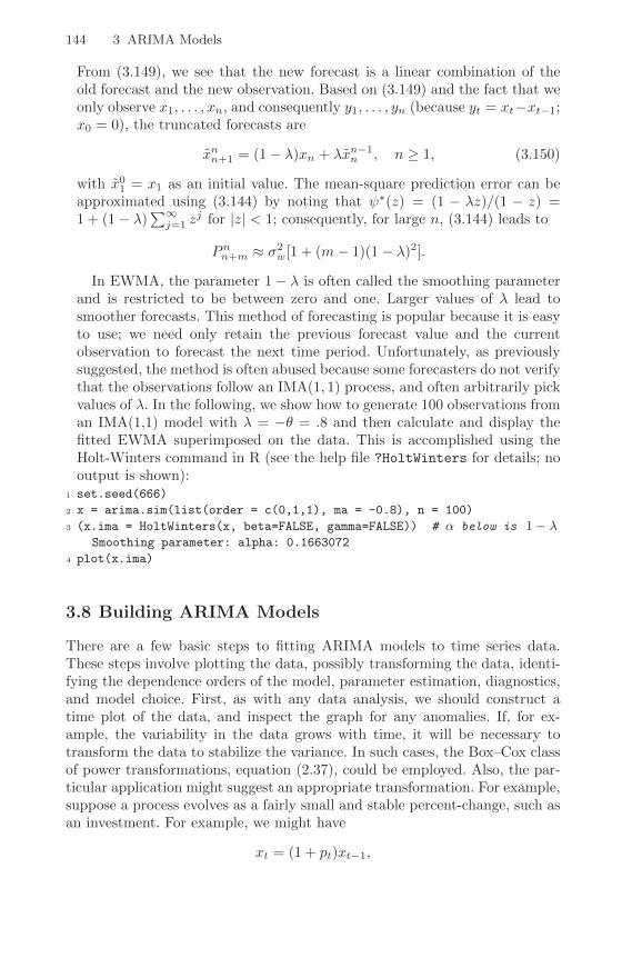
144 3 ARIMA Models
From (3.149), we see that the new forecast is a linear combination of theold forecast and the new observation. Based on (3.149) and the fact that weonly observe x1, . . . , xn, and consequently y1, . . . , yn (because yt = xt−xt−1;x0 = 0), the truncated forecasts are
xnn+1 = (1− λ)xn + λxn−1n , n ≥ 1, (3.150)
with x01 = x1 as an initial value. The mean-square prediction error can beapproximated using (3.144) by noting that ψ∗(z) = (1 − λz)/(1 − z) =1 + (1− λ)
∑∞j=1 z
j for |z| < 1; consequently, for large n, (3.144) leads to
Pnn+m ≈ σ2w[1 + (m− 1)(1− λ)2].
In EWMA, the parameter 1− λ is often called the smoothing parameterand is restricted to be between zero and one. Larger values of λ lead tosmoother forecasts. This method of forecasting is popular because it is easyto use; we need only retain the previous forecast value and the currentobservation to forecast the next time period. Unfortunately, as previouslysuggested, the method is often abused because some forecasters do not verifythat the observations follow an IMA(1, 1) process, and often arbitrarily pickvalues of λ. In the following, we show how to generate 100 observations froman IMA(1,1) model with λ = −θ = .8 and then calculate and display thefitted EWMA superimposed on the data. This is accomplished using theHolt-Winters command in R (see the help file ?HoltWinters for details; nooutput is shown):
1 set.seed(666)
2 x = arima.sim(list(order = c(0,1,1), ma = -0.8), n = 100)
3 (x.ima = HoltWinters(x, beta=FALSE, gamma=FALSE)) # α below is 1− λSmoothing parameter: alpha: 0.1663072
4 plot(x.ima)
3.8 Building ARIMA Models
There are a few basic steps to fitting ARIMA models to time series data.These steps involve plotting the data, possibly transforming the data, identi-fying the dependence orders of the model, parameter estimation, diagnostics,and model choice. First, as with any data analysis, we should construct atime plot of the data, and inspect the graph for any anomalies. If, for ex-ample, the variability in the data grows with time, it will be necessary totransform the data to stabilize the variance. In such cases, the Box–Cox classof power transformations, equation (2.37), could be employed. Also, the par-ticular application might suggest an appropriate transformation. For example,suppose a process evolves as a fairly small and stable percent-change, such asan investment. For example, we might have
xt = (1 + pt)xt−1,
3.8 Building ARIMA Models 145
where xt is the value of the investment at time t and pt is the percentage-change from period t− 1 to t, which may be negative. Taking logs we have
log(xt) = log(1 + pt) + log(xt−1),
or∇ log(xt) = log(1 + pt).
If the percent change pt stays relatively small in magnitude, then log(1+pt) ≈pt
8 and, thus,∇ log(xt) ≈ pt,
will be a relatively stable process. Frequently, ∇ log(xt) is called the returnor growth rate. This general idea was used in Example 3.32, and we will useit again in Example 3.38.
After suitably transforming the data, the next step is to identify prelim-inary values of the autoregressive order, p, the order of differencing, d, andthe moving average order, q. We have already addressed, in part, the problemof selecting d. A time plot of the data will typically suggest whether any dif-ferencing is needed. If differencing is called for, then difference the data once,d = 1, and inspect the time plot of ∇xt. If additional differencing is necessary,then try differencing again and inspect a time plot of ∇2xt. Be careful notto overdifference because this may introduce dependence where none exists.For example, xt = wt is serially uncorrelated, but ∇xt = wt−wt−1 is MA(1).In addition to time plots, the sample ACF can help in indicating whetherdifferencing is needed. Because the polynomial φ(z)(1 − z)d has a unit root,the sample ACF, ρ(h), will not decay to zero fast as h increases. Thus, a slowdecay in ρ(h) is an indication that differencing may be needed.
When preliminary values of d have been settled, the next step is to look atthe sample ACF and PACF of ∇dxt for whatever values of d have been chosen.Using Table 3.1 as a guide, preliminary values of p and q are chosen. Recallthat, if p = 0 and q > 0, the ACF cuts off after lag q, and the PACF tails off.If q = 0 and p > 0, the PACF cuts off after lag p, and the ACF tails off. Ifp > 0 and q > 0, both the ACF and PACF will tail off. Because we are dealingwith estimates, it will not always be clear whether the sample ACF or PACFis tailing off or cutting off. Also, two models that are seemingly different canactually be very similar. With this in mind, we should not worry about beingso precise at this stage of the model fitting. At this stage, a few preliminaryvalues of p, d, and q should be at hand, and we can start estimating theparameters.
Example 3.38 Analysis of GNP Data
In this example, we consider the analysis of quarterly U.S. GNP from1947(1) to 2002(3), n = 223 observations. The data are real U.S. gross
8 log(1 +p) = p− p2
2+ p3
3−· · · for −1 < p ≤ 1. If p is a small percent-change, then
the higher-order terms in the expansion are negligible.

146 3 ARIMA Models
Time
gnp
1950 1960 1970 1980 1990 2000
2000
4000
6000
8000
Fig. 3.12. Quarterly U.S. GNP from 1947(1) to 2002(3).
0 2 4 6 8 10 12
0.0
0.2
0.4
0.6
0.8
1.0
Lag
ACF
Fig. 3.13. Sample ACF of the GNP data. Lag is in terms of years.
national product in billions of chained 1996 dollars and have been season-ally adjusted. The data were obtained from the Federal Reserve Bank ofSt. Louis (http://research.stlouisfed.org/). Figure 3.12 shows a plotof the data, say, yt. Because strong trend hides any other effect, it is notclear from Figure 3.12 that the variance is increasing with time. For thepurpose of demonstration, the sample ACF of the data is displayed in Fig-ure 3.13. Figure 3.14 shows the first difference of the data, ∇yt, and nowthat the trend has been removed we are able to notice that the variability inthe second half of the data is larger than in the first half of the data. Also,it appears as though a trend is still present after differencing. The growth

3.8 Building ARIMA Models 147
Time
diff(
gnp)
1950 1960 1970 1980 1990 2000
−100
−50
050
100
150
Fig. 3.14. First difference of the U.S. GNP data.
Time
gnpg
r
1950 1960 1970 1980 1990 2000
−0.0
20.
000.
020.
04
Fig. 3.15. U.S. GNP quarterly growth rate.
rate, say, xt = ∇ log(yt), is plotted in Figure 3.15, and, appears to be a sta-ble process. Moreover, we may interpret the values of xt as the percentagequarterly growth of U.S. GNP.
The sample ACF and PACF of the quarterly growth rate are plotted inFigure 3.16. Inspecting the sample ACF and PACF, we might feel that theACF is cutting off at lag 2 and the PACF is tailing off. This would suggestthe GNP growth rate follows an MA(2) process, or log GNP follows anARIMA(0, 1, 2) model. Rather than focus on one model, we will also suggestthat it appears that the ACF is tailing off and the PACF is cutting off at

148 3 ARIMA Models
1 2 3 4 5 6
−0.2
0.4
0.8
LAG
ACF
1 2 3 4 5 6
−0.2
0.4
0.8
LAG
PAC
F
Fig. 3.16. Sample ACF and PACF of the GNP quarterly growth rate. Lag is interms of years.
lag 1. This suggests an AR(1) model for the growth rate, or ARIMA(1, 1, 0)for log GNP. As a preliminary analysis, we will fit both models.
Using MLE to fit the MA(2) model for the growth rate, xt, the estimatedmodel is
xt = .008(.001) + .303(.065)wt−1 + .204(.064)wt−2 + wt, (3.151)
where σw = .0094 is based on 219 degrees of freedom. The values in paren-theses are the corresponding estimated standard errors. All of the regressioncoefficients are significant, including the constant. We make a special note ofthis because, as a default, some computer packages do not fit a constant ina differenced model. That is, these packages assume, by default, that thereis no drift. In this example, not including a constant leads to the wrongconclusions about the nature of the U.S. economy. Not including a constantassumes the average quarterly growth rate is zero, whereas the U.S. GNPaverage quarterly growth rate is about 1% (which can be seen easily in Fig-ure 3.15). We leave it to the reader to investigate what happens when theconstant is not included.
The estimated AR(1) model is
xt = .008(.001) (1− .347) + .347(.063)xt−1 + wt, (3.152)
where σw = .0095 on 220 degrees of freedom; note that the constant in(3.152) is .008 (1− .347) = .005.
We will discuss diagnostics next, but assuming both of these models fitwell, how are we to reconcile the apparent differences of the estimated models
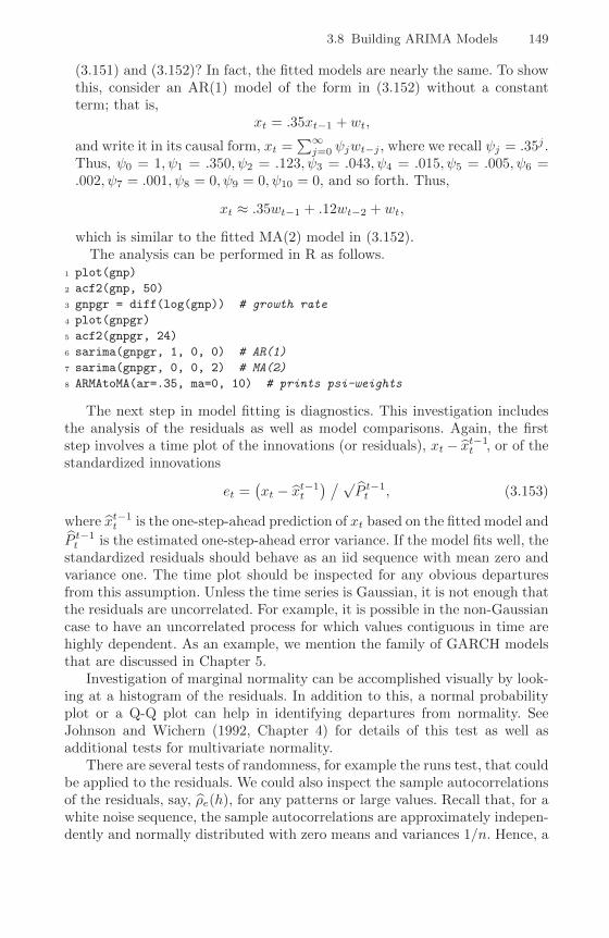
3.8 Building ARIMA Models 149
(3.151) and (3.152)? In fact, the fitted models are nearly the same. To showthis, consider an AR(1) model of the form in (3.152) without a constantterm; that is,
xt = .35xt−1 + wt,
and write it in its causal form, xt =∑∞j=0 ψjwt−j , where we recall ψj = .35j .
Thus, ψ0 = 1, ψ1 = .350, ψ2 = .123, ψ3 = .043, ψ4 = .015, ψ5 = .005, ψ6 =.002, ψ7 = .001, ψ8 = 0, ψ9 = 0, ψ10 = 0, and so forth. Thus,
xt ≈ .35wt−1 + .12wt−2 + wt,
which is similar to the fitted MA(2) model in (3.152).The analysis can be performed in R as follows.
1 plot(gnp)
2 acf2(gnp, 50)
3 gnpgr = diff(log(gnp)) # growth rate
4 plot(gnpgr)
5 acf2(gnpgr, 24)
6 sarima(gnpgr, 1, 0, 0) # AR(1)
7 sarima(gnpgr, 0, 0, 2) # MA(2)
8 ARMAtoMA(ar=.35, ma=0, 10) # prints psi-weights
The next step in model fitting is diagnostics. This investigation includesthe analysis of the residuals as well as model comparisons. Again, the firststep involves a time plot of the innovations (or residuals), xt − xt−1t , or of thestandardized innovations
et =(xt − xt−1t
) / √P t−1t , (3.153)
where xt−1t is the one-step-ahead prediction of xt based on the fitted model and
P t−1t is the estimated one-step-ahead error variance. If the model fits well, thestandardized residuals should behave as an iid sequence with mean zero andvariance one. The time plot should be inspected for any obvious departuresfrom this assumption. Unless the time series is Gaussian, it is not enough thatthe residuals are uncorrelated. For example, it is possible in the non-Gaussiancase to have an uncorrelated process for which values contiguous in time arehighly dependent. As an example, we mention the family of GARCH modelsthat are discussed in Chapter 5.
Investigation of marginal normality can be accomplished visually by look-ing at a histogram of the residuals. In addition to this, a normal probabilityplot or a Q-Q plot can help in identifying departures from normality. SeeJohnson and Wichern (1992, Chapter 4) for details of this test as well asadditional tests for multivariate normality.
There are several tests of randomness, for example the runs test, that couldbe applied to the residuals. We could also inspect the sample autocorrelationsof the residuals, say, ρe(h), for any patterns or large values. Recall that, for awhite noise sequence, the sample autocorrelations are approximately indepen-dently and normally distributed with zero means and variances 1/n. Hence, a

150 3 ARIMA Models
good check on the correlation structure of the residuals is to plot ρe(h) versush along with the error bounds of ±2/
√n. The residuals from a model fit,
however, will not quite have the properties of a white noise sequence and thevariance of ρe(h) can be much less than 1/n. Details can be found in Box andPierce (1970) and McLeod (1978). This part of the diagnostics can be viewedas a visual inspection of ρe(h) with the main concern being the detection ofobvious departures from the independence assumption.
In addition to plotting ρe(h), we can perform a general test that takes intoconsideration the magnitudes of ρe(h) as a group. For example, it may be thecase that, individually, each ρe(h) is small in magnitude, say, each one is justslightly less that 2/
√n in magnitude, but, collectively, the values are large.
The Ljung–Box–Pierce Q-statistic given by
Q = n(n+ 2)
H∑h=1
ρ2e(h)
n− h(3.154)
can be used to perform such a test. The value H in (3.154) is chosen somewhatarbitrarily, typically, H = 20. Under the null hypothesis of model adequacy,asymptotically (n → ∞), Q ∼ χ2
H−p−q. Thus, we would reject the null hy-
pothesis at level α if the value of Q exceeds the (1−α)-quantile of the χ2H−p−q
distribution. Details can be found in Box and Pierce (1970), Ljung and Box(1978), and Davies et al. (1977). The basic idea is that if wt is white noise,then by Property 1.1, nρ2w(h), for h = 1, . . . ,H, are asymptotically indepen-
dent χ21 random variables. This means that n
∑Hh=1 ρ
2w(h) is approximately a
χ2H random variable. Because the test involves the ACF of residuals from a
model fit, there is a loss of p+q degrees of freedom; the other values in (3.154)are used to adjust the statistic to better match the asymptotic chi-squareddistribution.
Example 3.39 Diagnostics for GNP Growth Rate Example
We will focus on the MA(2) fit from Example 3.38; the analysis of the AR(1)residuals is similar. Figure 3.17 displays a plot of the standardized residuals,the ACF of the residuals, a boxplot of the standardized residuals, and thep-values associated with the Q-statistic, (3.154), at lags H = 3 throughH = 20 (with corresponding degrees of freedom H − 2).
Inspection of the time plot of the standardized residuals in Figure 3.17shows no obvious patterns. Notice that there are outliers, however, witha few values exceeding 3 standard deviations in magnitude. The ACF ofthe standardized residuals shows no apparent departure from the modelassumptions, and the Q-statistic is never significant at the lags shown. Thenormal Q-Q plot of the residuals shows departure from normality at thetails due to the outliers that occurred primarily in the 1950s and the early1980s.
The model appears to fit well except for the fact that a distribution withheavier tails than the normal distribution should be employed. We discuss

3.8 Building ARIMA Models 151
Standardized Residuals
Time
1950 1960 1970 1980 1990 2000
−3−1
13
1 2 3 4 5 6
−0.2
0.0
0.2
0.4
ACF of Residuals
LAG
ACF
−3 −2 −1 0 1 2 3
−3−1
13
Normal Q−Q Plot of Std Residuals
Theoretical QuantilesSa
mpl
e Q
uant
iles
5 10 15 20
0.0
0.4
0.8
p values for Ljung−Box statistic
lag
p va
lue
Fig. 3.17. Diagnostics of the residuals from MA(2) fit on GNP growth rate.
some possibilities in Chapters 5 and 6. The diagnostics shown in Figure 3.17are a by-product of the sarima command from the previous example.9
Example 3.40 Diagnostics for the Glacial Varve Series
In Example 3.32, we fit an ARIMA(0, 1, 1) model to the logarithms of theglacial varve data and there appears to be a small amount of autocorrelationleft in the residuals and the Q-tests are all significant; see Figure 3.18.
To adjust for this problem, we fit an ARIMA(1, 1, 1) to the logged varvedata and obtained the estimates
φ = .23(.05), θ = −.89(.03), σ2w = .23.
Hence the AR term is significant. The Q-statistic p-values for this model arealso displayed in Figure 3.18, and it appears this model fits the data well.
As previously stated, the diagnostics are byproducts of the individualsarima runs. We note that we did not fit a constant in either model because
9 The script tsdiag is available in R to run diagnostics for an ARIMA object,however, the script has errors and we do not recommend using it.
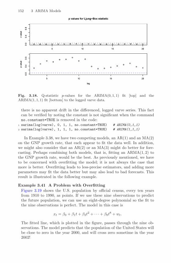
152 3 ARIMA Models
Fig. 3.18. Q-statistic p-values for the ARIMA(0, 1, 1) fit [top] and theARIMA(1, 1, 1) fit [bottom] to the logged varve data.
there is no apparent drift in the differenced, logged varve series. This factcan be verified by noting the constant is not significant when the commandno.constant=TRUE is removed in the code:
1 sarima(log(varve), 0, 1, 1, no.constant=TRUE) # ARIMA(0,1,1)
2 sarima(log(varve), 1, 1, 1, no.constant=TRUE) # ARIMA(1,1,1)
In Example 3.38, we have two competing models, an AR(1) and an MA(2)on the GNP growth rate, that each appear to fit the data well. In addition,we might also consider that an AR(2) or an MA(3) might do better for fore-casting. Perhaps combining both models, that is, fitting an ARMA(1, 2) tothe GNP growth rate, would be the best. As previously mentioned, we haveto be concerned with overfitting the model; it is not always the case thatmore is better. Overfitting leads to less-precise estimators, and adding moreparameters may fit the data better but may also lead to bad forecasts. Thisresult is illustrated in the following example.
Example 3.41 A Problem with Overfitting
Figure 3.19 shows the U.S. population by official census, every ten yearsfrom 1910 to 1990, as points. If we use these nine observations to predictthe future population, we can use an eight-degree polynomial so the fit tothe nine observations is perfect. The model in this case is
xt = β0 + β1t+ β2t2 + · · ·+ β8t
8 + wt.
The fitted line, which is plotted in the figure, passes through the nine ob-servations. The model predicts that the population of the United States willbe close to zero in the year 2000, and will cross zero sometime in the year2002!
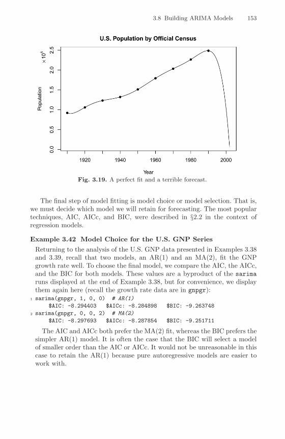
3.8 Building ARIMA Models 153
Fig. 3.19. A perfect fit and a terrible forecast.
The final step of model fitting is model choice or model selection. That is,we must decide which model we will retain for forecasting. The most populartechniques, AIC, AICc, and BIC, were described in §2.2 in the context ofregression models.
Example 3.42 Model Choice for the U.S. GNP Series
Returning to the analysis of the U.S. GNP data presented in Examples 3.38and 3.39, recall that two models, an AR(1) and an MA(2), fit the GNPgrowth rate well. To choose the final model, we compare the AIC, the AICc,and the BIC for both models. These values are a byproduct of the sarima
runs displayed at the end of Example 3.38, but for convenience, we displaythem again here (recall the growth rate data are in gnpgr):
1 sarima(gnpgr, 1, 0, 0) # AR(1)
$AIC: -8.294403 $AICc: -8.284898 $BIC: -9.263748
2 sarima(gnpgr, 0, 0, 2) # MA(2)
$AIC: -8.297693 $AICc: -8.287854 $BIC: -9.251711
The AIC and AICc both prefer the MA(2) fit, whereas the BIC prefers thesimpler AR(1) model. It is often the case that the BIC will select a modelof smaller order than the AIC or AICc. It would not be unreasonable in thiscase to retain the AR(1) because pure autoregressive models are easier towork with.
154 3 ARIMA Models
3.9 Multiplicative Seasonal ARIMA Models
In this section, we introduce several modifications made to the ARIMA modelto account for seasonal and nonstationary behavior. Often, the dependenceon the past tends to occur most strongly at multiples of some underlyingseasonal lag s. For example, with monthly economic data, there is a strongyearly component occurring at lags that are multiples of s = 12, becauseof the strong connections of all activity to the calendar year. Data takenquarterly will exhibit the yearly repetitive period at s = 4 quarters. Naturalphenomena such as temperature also have strong components correspondingto seasons. Hence, the natural variability of many physical, biological, andeconomic processes tends to match with seasonal fluctuations. Because of this,it is appropriate to introduce autoregressive and moving average polynomialsthat identify with the seasonal lags. The resulting pure seasonal autoregressivemoving average model, say, ARMA(P,Q)s, then takes the form
ΦP (Bs)xt = ΘQ(Bs)wt, (3.155)
with the following definition.
Definition 3.12 The operators
ΦP (Bs) = 1− Φ1Bs − Φ2B
2s − · · · − ΦPBPs (3.156)
andΘQ(Bs) = 1 +Θ1B
s +Θ2B2s + · · ·+ΘQB
Qs (3.157)
are the seasonal autoregressive operator and the seasonal moving av-erage operator of orders P and Q, respectively, with seasonal period s.
Analogous to the properties of nonseasonal ARMA models, the pure sea-sonal ARMA(P,Q)s is causal only when the roots of ΦP (zs) lie outside theunit circle, and it is invertible only when the roots of ΘQ(zs) lie outside theunit circle.
Example 3.43 A Seasonal ARMA Series
A first-order seasonal autoregressive moving average series that might runover months could be written as
(1− ΦB12)xt = (1 +ΘB12)wt
orxt = Φxt−12 + wt +Θwt−12.
This model exhibits the series xt in terms of past lags at the multiple of theyearly seasonal period s = 12 months. It is clear from the above form thatestimation and forecasting for such a process involves only straightforwardmodifications of the unit lag case already treated. In particular, the causalcondition requires |Φ| < 1, and the invertible condition requires |Θ| < 1.
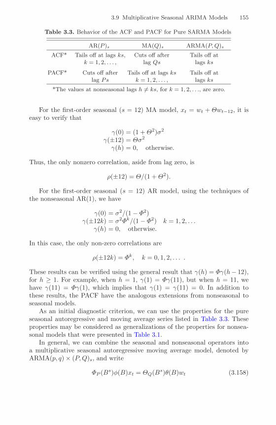
3.9 Multiplicative Seasonal ARIMA Models 155
Table 3.3. Behavior of the ACF and PACF for Pure SARMA Models
AR(P )s MA(Q)s ARMA(P,Q)s
ACF* Tails off at lags ks, Cuts off after Tails off atk = 1, 2, . . . , lag Qs lags ks
PACF* Cuts off after Tails off at lags ks Tails off atlag Ps k = 1, 2, . . . , lags ks
*The values at nonseasonal lags h 6= ks, for k = 1, 2, . . ., are zero.
For the first-order seasonal (s = 12) MA model, xt = wt + Θwt−12, it iseasy to verify that
γ(0) = (1 +Θ2)σ2
γ(±12) = Θσ2
γ(h) = 0, otherwise.
Thus, the only nonzero correlation, aside from lag zero, is
ρ(±12) = Θ/(1 +Θ2).
For the first-order seasonal (s = 12) AR model, using the techniques ofthe nonseasonal AR(1), we have
γ(0) = σ2/(1− Φ2)γ(±12k) = σ2Φk/(1− Φ2) k = 1, 2, . . .
γ(h) = 0, otherwise.
In this case, the only non-zero correlations are
ρ(±12k) = Φk, k = 0, 1, 2, . . . .
These results can be verified using the general result that γ(h) = Φγ(h− 12),for h ≥ 1. For example, when h = 1, γ(1) = Φγ(11), but when h = 11, wehave γ(11) = Φγ(1), which implies that γ(1) = γ(11) = 0. In addition tothese results, the PACF have the analogous extensions from nonseasonal toseasonal models.
As an initial diagnostic criterion, we can use the properties for the pureseasonal autoregressive and moving average series listed in Table 3.3. Theseproperties may be considered as generalizations of the properties for nonsea-sonal models that were presented in Table 3.1.
In general, we can combine the seasonal and nonseasonal operators intoa multiplicative seasonal autoregressive moving average model, denoted byARMA(p, q)× (P,Q)s, and write
ΦP (Bs)φ(B)xt = ΘQ(Bs)θ(B)wt (3.158)

156 3 ARIMA Models
as the overall model. Although the diagnostic properties in Table 3.3 arenot strictly true for the overall mixed model, the behavior of the ACF andPACF tends to show rough patterns of the indicated form. In fact, for mixedmodels, we tend to see a mixture of the facts listed in Tables 3.1 and 3.3.In fitting such models, focusing on the seasonal autoregressive and movingaverage components first generally leads to more satisfactory results.
Example 3.44 A Mixed Seasonal Model
Consider an ARMA(0, 1)× (1, 0)12 model
xt = Φxt−12 + wt + θwt−1,
where |Φ| < 1 and |θ| < 1. Then, because xt−12, wt, and wt−1 are uncorre-lated, and xt is stationary, γ(0) = Φ2γ(0) + σ2
w + θ2σ2w, or
γ(0) =1 + θ2
1− Φ2σ2w.
In addition, multiplying the model by xt−h, h > 0, and taking expectations,we have γ(1) = Φγ(11) + θσ2
w, and γ(h) = Φγ(h− 12), for h ≥ 2. Thus, theACF for this model is
ρ(12h) = Φh h = 1, 2, . . .
ρ(12h− 1) = ρ(12h+ 1) =θ
1 + θ2Φh h = 0, 1, 2, . . . ,
ρ(h) = 0, otherwise.
The ACF and PACF for this model, with Φ = .8 and θ = −.5, are shown inFigure 3.20. These type of correlation relationships, although idealized here,are typically seen with seasonal data.
To reproduce Figure 3.20 in R, use the following commands:1 phi = c(rep(0,11),.8)
2 ACF = ARMAacf(ar=phi, ma=-.5, 50)[-1] # [-1] removes 0 lag
3 PACF = ARMAacf(ar=phi, ma=-.5, 50, pacf=TRUE)
4 par(mfrow=c(1,2))
5 plot(ACF, type="h", xlab="lag", ylim=c(-.4,.8)); abline(h=0)
6 plot(PACF, type="h", xlab="lag", ylim=c(-.4,.8)); abline(h=0)
Seasonal nonstationarity can occur, for example, when the process is nearlyperiodic in the season. For example, with average monthly temperatures overthe years, each January would be approximately the same, each Februarywould be approximately the same, and so on. In this case, we might think ofaverage monthly temperature xt as being modeled as
xt = St + wt,
where St is a seasonal component that varies slowly from one year to the next,according to a random walk,

3.9 Multiplicative Seasonal ARIMA Models 157
0 10 20 30 40 50
−0.4
0.0
0.2
0.4
0.6
0.8
lag
ACF
0 10 20 30 40 50
−0.4
0.0
0.2
0.4
0.6
0.8
lag
PAC
FFig. 3.20. ACF and PACF of the mixed seasonal ARMA model xt = .8xt−12 +wt − .5wt−1.
St = St−12 + vt.
In this model, wt and vt are uncorrelated white noise processes. The tendencyof data to follow this type of model will be exhibited in a sample ACF that islarge and decays very slowly at lags h = 12k, for k = 1, 2, . . . . If we subtractthe effect of successive years from each other, we find that
(1−B12)xt = xt − xt−12 = vt + wt − wt−12.
This model is a stationary MA(1)12, and its ACF will have a peak only at lag12. In general, seasonal differencing can be indicated when the ACF decaysslowly at multiples of some season s, but is negligible between the periods.Then, a seasonal difference of order D is defined as
∇Ds xt = (1−Bs)Dxt, (3.159)
where D = 1, 2, . . ., takes positive integer values. Typically, D = 1 is sufficientto obtain seasonal stationarity. Incorporating these ideas into a general modelleads to the following definition.
Definition 3.13 The multiplicative seasonal autoregressive integratedmoving average model, or SARIMA model is given by
ΦP (Bs)φ(B)∇Ds ∇dxt = δ +ΘQ(Bs)θ(B)wt, (3.160)
where wt is the usual Gaussian white noise process. The general model isdenoted as ARIMA(p, d, q)× (P,D,Q)s. The ordinary autoregressive andmoving average components are represented by polynomials φ(B) and θ(B)of orders p and q, respectively [see (3.5) and (3.18)], and the seasonal autore-gressive and moving average components by ΦP (Bs) and ΘQ(Bs) [see (3.156)and (3.157)] of orders P and Q and ordinary and seasonal difference compo-nents by ∇d = (1−B)d and ∇Ds = (1−Bs)D.
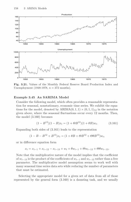
158 3 ARIMA Models
1950 1955 1960 1965 1970 1975
40
60
80
100
120
140
160Production
1950 1955 1960 1965 1970 19750
200
400
600
800
1000
Unemployment
Fig. 3.21. Values of the Monthly Federal Reserve Board Production Index andUnemployment (1948-1978, n = 372 months).
Example 3.45 An SARIMA Model
Consider the following model, which often provides a reasonable representa-tion for seasonal, nonstationary, economic time series. We exhibit the equa-tions for the model, denoted by ARIMA(0, 1, 1)× (0, 1, 1)12 in the notationgiven above, where the seasonal fluctuations occur every 12 months. Then,the model (3.160) becomes
(1−B12)(1−B)xt = (1 +ΘB12)(1 + θB)wt. (3.161)
Expanding both sides of (3.161) leads to the representation
(1−B −B12 +B13)xt = (1 + θB +ΘB12 +ΘθB13)wt,
or in difference equation form
xt = xt−1 + xt−12 − xt−13 + wt + θwt−1 +Θwt−12 +Θθwt−13.
Note that the multiplicative nature of the model implies that the coefficientof wt−13 is the product of the coefficients of wt−1 and wt−12 rather than a freeparameter. The multiplicative model assumption seems to work well withmany seasonal time series data sets while reducing the number of parametersthat must be estimated.
Selecting the appropriate model for a given set of data from all of thoserepresented by the general form (3.160) is a daunting task, and we usually

3.9 Multiplicative Seasonal ARIMA Models 159
0 1 2 3 4
−0.2
0.2
0.6
1.0
LAG
ACF
0 1 2 3 4
−0.2
0.2
0.6
1.0
LAG
PACF
Fig. 3.22. ACF and PACF of the production series.
think first in terms of finding difference operators that produce a roughlystationary series and then in terms of finding a set of simple autoregressivemoving average or multiplicative seasonal ARMA to fit the resulting residualseries. Differencing operations are applied first, and then the residuals areconstructed from a series of reduced length. Next, the ACF and the PACF ofthese residuals are evaluated. Peaks that appear in these functions can oftenbe eliminated by fitting an autoregressive or moving average component inaccordance with the general properties of Tables 3.1 and 3.2. In consideringwhether the model is satisfactory, the diagnostic techniques discussed in §3.8still apply.
Example 3.46 The Federal Reserve Board Production Index
A problem of great interest in economics involves first identifying a modelwithin the Box–Jenkins class for a given time series and then producingforecasts based on the model. For example, we might consider applyingthis methodology to the Federal Reserve Board Production Index shown inFigure 3.21. For demonstration purposes only, the ACF and PACF for thisseries are shown in Figure 3.22. We note that the trend in the data, the slowdecay in the ACF, and the fact that the PACF at the first lag is nearly 1,all indicate nonstationary behavior.
Following the recommended procedure, a first difference was taken, andthe ACF and PACF of the first difference
∇xt = xt − xt−1

160 3 ARIMA Models
0 1 2 3 4
−0.2
0.2
0.6
1.0
LAG
ACF
0 1 2 3 4
−0.2
0.2
0.6
1.0
LAG
PACF
Fig. 3.23. ACF and PACF of differenced production, (1−B)xt.
are shown in Figure 3.23. Noting the peaks at seasonal lags, h = 1s, 2s, 3s, 4swhere s = 12 (i.e., h = 12, 24, 36, 48) with relatively slow decay suggests aseasonal difference. Figure 3.24 shows the ACF and PACF of the seasonaldifference of the differenced production, say,
∇12∇xt = (1−B12)(1−B)xt.
First, concentrating on the seasonal (s = 12) lags, the characteristics ofthe ACF and PACF of this series tend to show a strong peak at h = 1s inthe autocorrelation function, with smaller peaks appearing at h = 2s, 3s,combined with peaks at h = 1s, 2s, 3s, 4s in the partial autocorrelationfunction. It appears that either(i) the ACF is cutting off after lag 1s and the PACF is tailing off in the
seasonal lags,(ii) the ACF is cutting off after lag 3s and the PACF is tailing off in the
seasonal lags, or(iii) the ACF and PACF are both tailing off in the seasonal lags.Using Table 3.3, this suggests either (i) an SMA of order Q = 1, (ii) anSMA of order Q = 3, or (iii) an SARMA of orders P = 2 (because of thetwo spikes in the PACF) and Q = 1.
Next, inspecting the ACF and the PACF at the within season lags, h =1, . . . , 11, it appears that either (a) both the ACF and PACF are tailingoff, or (b) that the PACF cuts off at lag 2. Based on Table 3.1, this resultindicates that we should either consider fitting a model (a) with both p > 0and q > 0 for the nonseasonal components, say p = 1, q = 1, or (b) p =
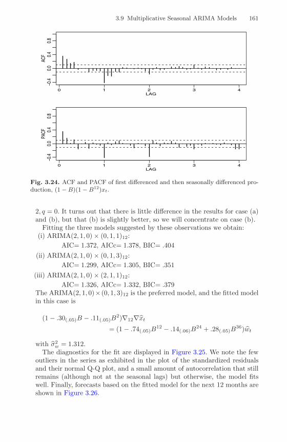
3.9 Multiplicative Seasonal ARIMA Models 161
0 1 2 3 4
−0.4
0.0
0.4
0.8
LAG
ACF
0 1 2 3 4
−0.4
0.0
0.4
0.8
LAG
PACF
Fig. 3.24. ACF and PACF of first differenced and then seasonally differenced pro-duction, (1−B)(1−B12)xt.
2, q = 0. It turns out that there is little difference in the results for case (a)and (b), but that (b) is slightly better, so we will concentrate on case (b).
Fitting the three models suggested by these observations we obtain:(i) ARIMA(2, 1, 0)× (0, 1, 1)12:
AIC= 1.372, AICc= 1.378, BIC= .404
(ii) ARIMA(2, 1, 0)× (0, 1, 3)12:
AIC= 1.299, AICc= 1.305, BIC= .351
(iii) ARIMA(2, 1, 0)× (2, 1, 1)12:
AIC= 1.326, AICc= 1.332, BIC= .379The ARIMA(2, 1, 0)× (0, 1, 3)12 is the preferred model, and the fitted modelin this case is
(1− .30(.05)B − .11(.05)B2)∇12∇xt
= (1− .74(.05)B12 − .14(.06)B
24 + .28(.05)B36)wt
with σ2w = 1.312.
The diagnostics for the fit are displayed in Figure 3.25. We note the fewoutliers in the series as exhibited in the plot of the standardized residualsand their normal Q-Q plot, and a small amount of autocorrelation that stillremains (although not at the seasonal lags) but otherwise, the model fitswell. Finally, forecasts based on the fitted model for the next 12 months areshown in Figure 3.26.

162 3 ARIMA Models
Fig. 3.25. Diagnostics for the ARIMA(2, 1, 0) × (0, 1, 3)12 fit on the ProductionIndex.
The following R code can be used to perform the analysis.1 acf2(prodn, 48)
2 acf2(diff(prodn), 48)
3 acf2(diff(diff(prodn), 12), 48)
4 sarima(prodn, 2, 1, 1, 0, 1, 3, 12) # fit model (ii)
5 sarima.for(prodn, 12, 2, 1, 1, 0, 1, 3, 12) # forecast
Problems
Section 3.2
3.1 For an MA(1), xt = wt + θwt−1, show that |ρx(1)| ≤ 1/2 for any numberθ. For which values of θ does ρx(1) attain its maximum and minimum?
3.2 Let wt be white noise with variance σ2w and let |φ| < 1 be a constant.
Consider the process x1 = w1, and
xt = φxt−1 + wt, t = 2, 3, . . . .

Problems 163
Fig. 3.26. Forecasts and limits for production index. The vertical dotted line sep-arates the data from the predictions.
(a) Find the mean and the variance of {xt, t = 1, 2, . . .}. Is xt stationary?(b) Show
corr(xt, xt−h) = φh[
var(xt−h)
var(xt)
]1/2for h ≥ 0.
(c) Argue that for large t,
var(xt) ≈σ2w
1− φ2
andcorr(xt, xt−h) ≈ φh, h ≥ 0,
so in a sense, xt is “asymptotically stationary.”(d) Comment on how you could use these results to simulate n observations
of a stationary Gaussian AR(1) model from simulated iid N(0,1) values.
(e) Now suppose x1 = w1/√
1− φ2. Is this process stationary?
3.3 Verify the calculations made in Example 3.3:
(a) Let xt = φxt−1 +wt where |φ| > 1 and wt ∼ iid N(0, σ2w). Show E(xt) = 0
and γx(h) = σ2wφ−2 φ−h/(1− φ−2).
(b) Let yt = φ−1yt−1 + vt where vt ∼ iid N(0, σ2wφ−2) and φ and σw are
as in part (a). Argue that yt is causal with the same mean function andautocovariance function as xt.
164 3 ARIMA Models
3.4 Identify the following models as ARMA(p, q) models (watch out for pa-rameter redundancy), and determine whether they are causal and/or invert-ible:
(a) xt = .80xt−1 − .15xt−2 + wt − .30wt−1.(b)xt = xt−1 − .50xt−2 + wt − wt−1.
3.5 Verify the causal conditions for an AR(2) model given in (3.28). That is,show that an AR(2) is causal if and only if (3.28) holds.
Section 3.3
3.6 For the AR(2) model given by xt = −.9xt−2 + wt, find the roots of theautoregressive polynomial, and then sketch the ACF, ρ(h).
3.7 For the AR(2) series shown below, use the results of Example 3.9 todetermine a set of difference equations that can be used to find the ACFρ(h), h = 0, 1, . . .; solve for the constants in the ACF using the initial condi-tions. Then plot the ACF values to lag 10 (use ARMAacf as a check on youranswers).
(a) xt + 1.6xt−1 + .64xt−2 = wt.(b)xt − .40xt−1 − .45xt−2 = wt.(c) xt − 1.2xt−1 + .85xt−2 = wt.
Section 3.4
3.8 Verify the calculations for the autocorrelation function of an ARMA(1, 1)process given in Example 3.13. Compare the form with that of the ACF forthe ARMA(1, 0) and the ARMA(0, 1) series. Plot (or sketch) the ACFs ofthe three series on the same graph for φ = .6, θ = .9, and comment on thediagnostic capabilities of the ACF in this case.
3.9 Generate n = 100 observations from each of the three models discussed inProblem 3.8. Compute the sample ACF for each model and compare it to thetheoretical values. Compute the sample PACF for each of the generated seriesand compare the sample ACFs and PACFs with the general results given inTable 3.1.
Section 3.5
3.10 Let xt represent the cardiovascular mortality series (cmort) discussed inChapter 2, Example 2.2.
(a) Fit an AR(2) to xt using linear regression as in Example 3.17.(b) Assuming the fitted model in (a) is the true model, find the forecasts over
a four-week horizon, xnn+m, for m = 1, 2, 3, 4, and the corresponding 95%prediction intervals.

Problems 165
3.11 Consider the MA(1) series
xt = wt + θwt−1,
where wt is white noise with variance σ2w.
(a) Derive the minimum mean-square error one-step forecast based on theinfinite past, and determine the mean-square error of this forecast.
(b) Let xnn+1 be the truncated one-step-ahead forecast as given in (3.92). Showthat
E[(xn+1 − xnn+1)2
]= σ2(1 + θ2+2n).
Compare the result with (a), and indicate how well the finite approxima-tion works in this case.
3.12 In the context of equation (3.63), show that, if γ(0) > 0 and γ(h) → 0as h→∞, then Γn is positive definite.
3.13 Suppose xt is stationary with zero mean and recall the definition of thePACF given by (3.55) and (3.56). That is, let
εt = xt −h−1∑i=1
aixt−i
and
δt−h = xt−h −h−1∑j=1
bjxt−j
be the two residuals where {a1, . . . , ah−1} and {b1, . . . , bh−1} are chosen sothat they minimize the mean-squared errors
E[ε2t ] and E[δ2t−h].
The PACF at lag h was defined as the cross-correlation between εt and δt−h;that is,
φhh =E(εtδt−h)√E(ε2t )E(δ2t−h)
.
Let Rh be the h× h matrix with elements ρ(i− j), i, j = 1, . . . , h, and letρρρh = (ρ(1), ρ(2), . . . , ρ(h))′ be the vector of lagged autocorrelations, ρ(h) =corr(xt+h, xt). Let ρρρh = (ρ(h), ρ(h − 1), . . . , ρ(1))′ be the reversed vector. Inaddition, let xht denote the BLP of xt given {xt−1, . . . , xt−h}:
xht = αh1xt−1 + · · ·+ αhhxt−h,
as described in Property 3.3. Prove
166 3 ARIMA Models
φhh =ρ(h)− ρρρ′h−1R−1h−1ρρρh1− ρρρ′h−1R−1h−1ρρρh−1
= αhh.
In particular, this result proves Property 3.4.Hint: Divide the prediction equations [see (3.63)] by γ(0) and write the
matrix equation in the partitioned form as(Rh−1 ρρρh−1ρρρ′h−1 ρ(0)
)(ααα1
αhh
)=
(ρρρh−1ρ(h)
),
where the h × 1 vector of coefficients ααα = (αh1, . . . , αhh)′ is partitioned asααα = (ααα′1, αhh)′.
3.14 Suppose we wish to find a prediction function g(x) that minimizes
MSE = E[(y − g(x))2],
where x and y are jointly distributed random variables with density functionf(x, y).
(a) Show that MSE is minimized by the choice
g(x) = E(y∣∣ x).
Hint:
MSE =
∫ [∫(y − g(x))2f(y|x)dy
]f(x)dx.
(b) Apply the above result to the model
y = x2 + z,
where x and z are independent zero-mean normal variables with varianceone. Show that MSE = 1.
(c) Suppose we restrict our choices for the function g(x) to linear functions ofthe form
g(x) = a+ bx
and determine a and b to minimize MSE. Show that a = 1 and
b =E(xy)
E(x2)= 0
and MSE = 3. What do you interpret this to mean?
3.15 For an AR(1) model, determine the general form of the m-step-aheadforecast xtt+m and show
E[(xt+m − xtt+m)2] = σ2w
1− φ2m
1− φ2.

Problems 167
3.16 Consider the ARMA(1,1) model discussed in Example 3.7, equation(3.27); that is, xt = .9xt−1 + .5wt−1 + wt. Show that truncated predictionas defined in (3.91) is equivalent to truncated prediction using the recursiveformula (3.92).
3.17 Verify statement (3.87), that for a fixed sample size, the ARMA predic-tion errors are correlated.
Section 3.6
3.18 Fit an AR(2) model to the cardiovascular mortality series (cmort) dis-cussed in Chapter 2, Example 2.2. using linear regression and using Yule–Walker.
(a) Compare the parameter estimates obtained by the two methods.(b) Compare the estimated standard errors of the coefficients obtained by
linear regression with their corresponding asymptotic approximations, asgiven in Property 3.10.
3.19 Suppose x1, . . . , xn are observations from an AR(1) process with µ = 0.
(a) Show the backcasts can be written as xnt = φ1−tx1, for t ≤ 1.(b) In turn, show, for t ≤ 1, the backcasted errors are
wt(φ) = xnt − φxnt−1 = φ1−t(1− φ2)x1.
(c) Use the result of (b) to show∑1t=−∞ w2
t (φ) = (1− φ2)x21.(d) Use the result of (c) to verify the unconditional sum of squares, S(φ), can
be written as∑nt=−∞ w2
t (φ).
(e) Find xt−1t and rt for 1 ≤ t ≤ n, and show that
S(φ) =n∑t=1
(xt − xt−1t )2/rt.
3.20 Repeat the following numerical exercise three times. Generate n = 500observations from the ARMA model given by
xt = .9xt−1 + wt − .9wt−1,
with wt ∼ iid N(0, 1). Plot the simulated data, compute the sample ACF andPACF of the simulated data, and fit an ARMA(1, 1) model to the data. Whathappened and how do you explain the results?
3.21 Generate 10 realizations of length n = 200 each of an ARMA(1,1) processwith φ = .9, θ = .5 and σ2 = 1. Find the MLEs of the three parameters ineach case and compare the estimators to the true values.

168 3 ARIMA Models
3.22 Generate n = 50 observations from a Gaussian AR(1) model with φ =.99 and σw = 1. Using an estimation technique of your choice, compare theapproximate asymptotic distribution of your estimate (the one you would usefor inference) with the results of a bootstrap experiment (use B = 200).
3.23 Using Example 3.31 as your guide, find the Gauss–Newton proce-dure for estimating the autoregressive parameter, φ, from the AR(1) model,xt = φxt−1 + wt, given data x1, . . . , xn. Does this procedure produce the un-conditional or the conditional estimator? Hint: Write the model as wt(φ) =xt − φxt−1; your solution should work out to be a non-recursive procedure.
3.24 Consider the stationary series generated by
xt = α+ φxt−1 + wt + θwt−1,
where E(xt) = µ, |θ| < 1, |φ| < 1 and the wt are iid random variables withzero mean and variance σ2
w.
(a) Determine the mean as a function of α for the above model. Find theautocovariance and ACF of the process xt, and show that the process isweakly stationary. Is the process strictly stationary?
(b) Prove the limiting distribution as n→∞ of the sample mean,
x = n−1n∑t=1
xt,
is normal, and find its limiting mean and variance in terms of α, φ, θ, andσ2w. (Note: This part uses results from Appendix A.)
3.25 A problem of interest in the analysis of geophysical time series involvesa simple model for observed data containing a signal and a reflected version ofthe signal with unknown amplification factor a and unknown time delay δ. Forexample, the depth of an earthquake is proportional to the time delay δ forthe P wave and its reflected form pP on a seismic record. Assume the signal,say st, is white and Gaussian with variance σ2
s , and consider the generatingmodel
xt = st + ast−δ.
(a) Prove the process xt is stationary. If |a| < 1, show that
st =∞∑j=0
(−a)jxt−δj
is a mean square convergent representation for the signal st, for t =1,±1,±2, . . ..
(b) If the time delay δ is assumed to be known, suggest an approximate com-putational method for estimating the parameters a and σ2
s using maximumlikelihood and the Gauss–Newton method.

Problems 169
(c) If the time delay δ is an unknown integer, specify how we could estimatethe parameters including δ. Generate a n = 500 point series with a = .9,σ2w = 1 and δ = 5. Estimate the integer time delay δ by searching overδ = 3, 4, . . . , 7.
3.26 Forecasting with estimated parameters: Let x1, x2, . . . , xn be a sample ofsize n from a causal AR(1) process, xt = φxt−1+wt. Let φ be the Yule–Walkerestimator of φ.
(a) Show φ− φ = Op(n−1/2). See Appendix A for the definition of Op(·).
(b) Let xnn+1 be the one-step-ahead forecast of xn+1 given the data x1, . . . , xn,based on the known parameter, φ, and let xnn+1 be the one-step-ahead fore-
cast when the parameter is replaced by φ. Show xnn+1− xnn+1 = Op(n−1/2).
Section 3.7
3.27 Suppose
yt = β0 + β1t+ · · ·+ βqtq + xt, βq 6= 0,
where xt is stationary. First, show that∇kxt is stationary for any k = 1, 2, . . . ,and then show that ∇kyt is not stationary for k < q, but is stationary fork ≥ q.
3.28 Verify that the IMA(1,1) model given in (3.147) can be inverted andwritten as (3.148).
3.29 For the ARIMA(1, 1, 0) model with drift, (1 − φB)(1 − B)xt = δ + wt,let yt = (1−B)xt = ∇xt.(a) Noting that yt is AR(1), show that, for j ≥ 1,
ynn+j = δ [1 + φ+ · · ·+ φj−1] + φj yn.
(b) Use part (a) to show that, for m = 1, 2, . . . ,
xnn+m = xn +δ
1− φ
[m− φ(1− φm)
(1− φ)
]+ (xn − xn−1)
φ(1− φm)
(1− φ).
Hint: From (a), xnn+j − xnn+j−1 = δ 1−φj1−φ + φj(xn − xn−1). Now sum both
sides over j from 1 to m.(c) Use (3.144) to find Pnn+m by first showing that ψ∗0 = 1, ψ∗1 = (1 + φ), and
ψ∗j − (1 + φ)ψ∗j−1 + φψ∗j−2 = 0 for j ≥ 2, in which case ψ∗j = 1−φj+1
1−φ , for
j ≥ 1. Note that, as in Example 3.36, equation (3.144) is exact here.
3.30 For the logarithm of the glacial varve data, say, xt, presented in Example3.32, use the first 100 observations and calculate the EWMA, xtt+1, given in(3.150) for t = 1, . . . , 100, using λ = .25, .50, and .75, and plot the EWMAsand the data superimposed on each other. Comment on the results.
170 3 ARIMA Models
Section 3.8
3.31 In Example 3.39, we presented the diagnostics for the MA(2) fit to theGNP growth rate series. Using that example as a guide, complete the diag-nostics for the AR(1) fit.
3.32 Crude oil prices in dollars per barrel are in oil; see Appendix R formore details. Fit an ARIMA(p, d, q) model to the growth rate performing allnecessary diagnostics. Comment.
3.33 Fit an ARIMA(p, d, q) model to the global temperature data gtemp per-forming all of the necessary diagnostics. After deciding on an appropriatemodel, forecast (with limits) the next 10 years. Comment.
3.34 One of the series collected along with particulates, temperature, andmortality described in Example 2.2 is the sulfur dioxide series, so2. Fit anARIMA(p, d, q) model to the data, performing all of the necessary diagnostics.After deciding on an appropriate model, forecast the data into the future fourtime periods ahead (about one month) and calculate 95% prediction intervalsfor each of the four forecasts. Comment.
Section 3.9
3.35 Consider the ARIMA model
xt = wt +Θwt−2.
(a) Identify the model using the notation ARIMA(p, d, q)× (P,D,Q)s.(b) Show that the series is invertible for |Θ| < 1, and find the coefficients in
the representation
wt =∞∑k=0
πkxt−k.
(c) Develop equations for the m-step ahead forecast, xn+m, and its variancebased on the infinite past, xn, xn−1, . . . .
3.36 Plot (or sketch) the ACF of the seasonal ARIMA(0, 1)× (1, 0)12 modelwith Φ = .8 and θ = .5.
3.37 Fit a seasonal ARIMA model of your choice to the unemployment data(unemp) displayed in Figure 3.21. Use the estimated model to forecast thenext 12 months.
3.38 Fit a seasonal ARIMA model of your choice to the U.S. Live Birth Series(birth). Use the estimated model to forecast the next 12 months.
3.39 Fit an appropriate seasonal ARIMA model to the log-transformed John-son and Johnson earnings series (jj) of Example 1.1. Use the estimated modelto forecast the next 4 quarters.

Problems 171
The following problems require supplemental material given in Appendix B.
3.40 Suppose xt =∑pj=1 φjxt−j + wt, where φp 6= 0 and wt is white noise
such that wt is uncorrelated with {xk; k < t}. Use the Projection Theorem toshow that, for n > p, the BLP of xn+1 on sp{xk, k ≤ n} is
xn+1 =
p∑j=1
φjxn+1−j .
3.41 Use the Projection Theorem to derive the Innovations Algorithm, Prop-erty 3.6, equations (3.77)-(3.79). Then, use Theorem B.2 to derive the m-step-ahead forecast results given in (3.80) and (3.81).
3.42 Consider the series xt = wt−wt−1, where wt is a white noise process withmean zero and variance σ2
w. Suppose we consider the problem of predictingxn+1, based on only x1, . . . , xn. Use the Projection Theorem to answer thequestions below.
(a) Show the best linear predictor is
xnn+1 = − 1
n+ 1
n∑k=1
k xk.
(b) Prove the mean square error is
E(xn+1 − xnn+1)2 =n+ 2
n+ 1σ2w.
3.43 Use Theorem B.2 and B.3 to verify (3.116).
3.44 Prove Theorem B.2.
3.45 Prove Property 3.2.

Appendix RR Supplement
R.1 First Things First
If you do not already have R, point your browser to the Comprehensive RArchive Network (CRAN), http://cran.r-project.org/ and download andinstall it. The installation includes help files and some user manuals. You canfind helpful tutorials by following CRAN’s link to Contributed Documentation.If you are new to R/S-PLUS, then R for Beginners by Emmanuel Paradis isa great introduction. There is also a lot of advice out there in cyberspace, butsome of it will be outdated because R goes through many revisions.
Next, point your browser to http://www.stat.pitt.edu/stoffer/tsa3/,the website for the text, or one of its mirrors, download tsa3.rda and putit in a convenient place (e.g., the working directory of R).1 This file containsthe data sets and scripts that are used in the text. Then, start R and issuethe command
1 load("tsa3.rda")
Once you have loaded tsa3.rda, all the files will stay in R as long as yousave the workspace when you close R (details in §R.2). If you don’t save theworkspace, you will have to reload it. To see what is included in tsa3.rda
type
2 ls() # to get a listing of your objects, and
3 tsa3.version # to check the version
Periodically check that your version matches the latest version number (year-month-day) on the website. Please note that tsa3.rda is subject to change.
You are free to use the data or to alter the scripts in any way you see fit.We only have two requests: reference the text if you use something from it,and contact us if you find any errors or have suggestions for improvement ofthe code.
1 See §R.2, page 567, on how to get the current working directory and how tochange it, or page 569 on how to read files from other directories.
560 Appendix R: R Supplement
R.1.1 Included Data Sets
The data sets included in tsa3.rda, listed by the chapter in which they arefirst presented, are as follows.
Chapter 1jj - Johnson & Johnson quarterly earnings per share, 84 quarters (21
years) measured from the first quarter of 1960 to the last quarterof 1980.
EQ5 - Seismic trace of an earthquake [two phases or arrivals along thesurface, the primary wave (t = 1, . . . , 1024) and the shear wave(t = 1025, . . . , 2048)] recorded at a seismic station.
EXP6 - Seismic trace of an explosion (similar details as EQ5).gtemp - Global mean land-ocean temperature deviations (from 1951-1980
average), measured in degrees centigrade, for the years 1880-2009;data taken from http://data.giss.nasa.gov/gistemp/graphs/
fmri1 - A data frame that consists of fmri bold signals at eight locations(in columns 2-9, column 1 is time period), when a stimulus wasapplied for 32 seconds and then stopped for 32 seconds. The signalperiod is 64 seconds and the sampling rate was one observationevery 2 seconds for 256 seconds (n = 128).
soi - Southern Oscillation Index (SOI) for a period of 453 months rangingover the years 1950-1987.
rec - Recruitment (number of new fish) associated with SOI.speech - A small .1 second (1000 points) sample of recorded speech for the
phrase aaa · · ·hhh.nyse - Returns of the New York Stock Exchange (NYSE) from February
2, 1984 to December 31, 1991.soiltemp - A 64× 36 matrix of surface soil temperatures.
Chapter 2oil - Crude oil, WTI spot price FOB (in dollars per barrel), weekly
data from 2000 to mid-2010. For definitions and more details, seehttp://tonto.eia.doe.gov/dnav/pet/pet_pri_spt_s1_w.htm.
gas - New York Harbor conventional regular gasoline weekly spot priceFOB (in cents per gallon) over the same time period as oil.
varve - Sedimentary deposits from one location in Massachusetts for 634years, beginning nearly 12,000 years ago.
cmort - Average weekly cardiovascular mortality in Los Angeles County;508 six-day smoothed averages obtained by filtering daily valuesover the 10 year period 1970-1979.
tempr - Temperature series corresponding to cmort.part - Particulate series corresponding to cmort.so2 - Sulfur dioxide series corresponding to cmort.
Chapter 3prodn - Monthly Federal Reserve Board Production Index (1948-1978, n =
372 months).unemp - Unemployment series corresponding to prodn.ar1boot - Data used in Example 3.35 on page 137.
R.1.1 Included Data Sets 561
gnp - Quarterly U.S. GNP from 1947(1) to 2002(3), n = 223 observations.birth - Monthly live births (adjusted) in thousands for the United States,
1948-1979.
Chapter 4sunspotz - Biannual smoothed (12-month moving average) number of sunspots
from June 1749 to December 1978; n = 459. The “z” on the endis to distinguish this series from the one included with R (calledsunspots).
salt - Salt profiles taken over a spatial grid set out on an agriculturalfield, 64 rows at 17-ft spacing.
saltemp - Temperature profiles corresponding to salt.
Chapter 5arf - 1000 simulated observations from an ARFIMA(1, 1, 0) model with
φ = .75 and d = .4.flu - Monthly pneumonia and influenza deaths per 10,000 people in the
United States for 11 years, 1968 to 1978.sales - Sales (with lead, a leading indicator), 150 months; taken from Box
& Jenkins (1970).lead - See sales.econ5 - Data set containing quarterly U.S. unemployment, GNP, consump-
tion, and government and private investment, from 1948-III to 1988-II.
Chapter 6ar1miss - Data for Problem 6.14 on page 403.gtemp2 - Similar to gtemp but the data are based only on surface air tem-
perature data obtained from meteorological stations.qinfl - Quarterly inflation rate in the Consumer Price Index from 1953-I
to 1980-II, n = 110 observations; from Newbold and Bos (1985).qintr - Quarterly interest rate recorded for Treasury bills over the same
period as qinfl.WBC - Measurements made for 91 days on the three variables, log(white
blood count) [WBC], log(platelet) [PLT] and hematocrit [HCT]; takenfrom Jones (1984).
PLT - See WBC.HCT - See WBC.
Chapter 7beamd - Infrasonic signals from a nuclear explosion. This is a data frame
consisting of three columns (which are not time series objects) thatare data from different channels. The series names are sensor1,
sensor2, sensor3. See Example 7.2 on page 421 for more infor-mation.
bnrf1ebv - Nucleotide sequence of the BNRF1 gene of the Epstein-Barr virus(EBV): 1=A, 2=C, 3=G, 4=T. The data are used in §7.9.
bnrf1hvs - Nucleotide sequence of the BNRF1 gene of the herpes virus saimiri(HVS); same codes as for EBV.

562 Appendix R: R Supplement
fmri - Data (as a vector list) from an fMRI experiment in pain, listedby location and stimulus. The specfic locations of the brain wherethe signal was measured were [1] Cortex 1: Primary Somatosensory,Contralateral, [2] Cortex 2: Primary Somatosensory, Ipsilateral, [3]Cortex 3: Secondary Somatosensory, Contralateral, [4] Cortex 4:Secondary Somatosensory, Ipsilateral, [5] Caudate, [6] Thalamus 1:Contralateral, [7] Thalamus 2: Ipsilateral, [8] Cerebellum 1: Con-tralateral and [9] Cerebellum 2: Ipsilateral. The stimuli (and num-ber of subjects in each condition) are [1] Awake-Brush (5 subjects),[2] Awake-Heat (4 subjects), [3] Awake-Shock (5 subjects), [4] Low-Brush (3 subjects), [5] Low-Heat (5 subjects), and [6] Low-Shock(4 subjects). Issue the command summary(fmri) for further details.As an example, fmri$L1T6 (location 1, treatment 6) will show thedata for the four subjects receiving the Low-Shock treatment at theCortex 1 location; note that fmri[[6]] will display the same data.See Examples 7.7–7.9 for examples.
climhyd - Lake Shasta inflow data; see Example 7.1. This is a data frame withcolumn names: Temp, DewPt, CldCvr, WndSpd, Precip, Inflow.
eqexp - This is a data frame of the earthquake and explosion seismic seriesused throughout the text. The matrix has 17 columns, the firsteight are earthquakes, the second eight are explosions, and the lastcolumn is the Novaya Zemlya series. The column names are: EQ1,EQ2,...,EQ8; EX1, EX2,...,EX8; NZ.
R.1.2 Included Scripts
The following scripts are included in tsa3.rda. At the end of the descriptionof each script, a text example that demonstrates the use of the script is given.
lag.plot2(series1, series2, max.lag=0, corr=TRUE, smooth=TRUE)
Produces a grid of scatterplots of one series versus another. If (xt, yt) is a vector
time series, then lag.plot2(x,y,m) will generate a grid of scatterplots of xt−hversus yt for h = 0, 1, ...,m, along with the cross-correlation values (corr=TRUE)
and a lowess fit (smooth=TRUE) assuming xt is in x and yt is in y. Note that the first
series, xt, is the one that gets lagged. If you just want the scatterplots and nothing
else, then use lag.plot2(x,y,m,corr=FALSE,smooth=FALSE). See Example 2.7 on
page 64 for a demonstration.
lag.plot1(series, max.lag=1, corr=TRUE, smooth=TRUE)
Produces a grid of scatterplots of a series versus lagged values of the series. Sim-
ilar to lag.plot2, the call lag.plot1(x,m) will generate a grid of scatterplots of
xt−h versus xt for h = 1, ...,m, along with the autocorrelation values (corr=TRUE)
and a lowess fit (smooth=TRUE). The defaults are the same as lag.plot2; if you
don’t want either the correlation values or the lowess fit, you can either use
lag.plot1(x,m,corr=FALSE,smooth=FALSE) or R’s lag.plot. See Example 2.7
on page 64 for a demonstration.

R.1.2 Included Scripts 563
acf2(series, max.lag=NULL)
Produces a simultaneous plot (and a printout) of the sample ACF and PACF on
the same scale. If x contains n observations, acf2(x) will print and plot the ACF
and PACF of x to the default lag of√n + 10 (unless n is smaller than 50). The
number of lags may be specified, e.g., acf2(x, 33). See Example 3.17 on page 108.
sarima(series, p, d, q, P=0, D=0, Q=0, S=-1, details=TRUE,
tol=sqrt(.Machine$double.eps), no.constant=FALSE)
Fits ARIMA models including diagnostics in a short command. If your time se-ries is in x and you want to fit an ARIMA(p, d, q) model to the data, the ba-sic call is sarima(x,p,d,q). The results are the parameter estimates, standarderrors, AIC, AICc, BIC (as defined in Chapter 2) and diagnostics. To fit a sea-sonal ARIMA model, the basic call is sarima(x,p,d,q,P,D,Q,S). So, for exam-ple, sarima(x,2,1,0) will fit an ARIMA(2, 1, 0) model to the series in x, andsarima(x,2,1,0,0,1,1,12) will fit a seasonal ARIMA(2, 1, 0) × (0, 1, 1)12 modelto the series in x. If you want to look at the innovations (i.e., the residuals) fromthe fit, they’re stored in innov.
There are three additional options that can be included in the call.• details turns on/off the output from the nonlinear optimization routine,
which is optim. The default is TRUE, use details=FALSE to turn off the output;e.g., sarima(x,2,1,0,details=FALSE).
• tol controls the relative tolerance (reltol) used to assess convergence in sarima
and sarima.for. The default is tol=sqrt(.Machine$double.eps), the R de-fault. For details, see the help file for optim under the control arguments.For example, sarima(rec,2,0,0,tol=.0001) will speed up the convergence.If there are many parameters to estimate (e.g., seasonal models), the analysismay take a long time using the default.
• no.constant can control whether or not sarima includes a constant in themodel. In particular, with sarima, if there is no differencing (d = 0 and D = 0)you get the mean estimate. If there’s differencing of order one (either d = 1 orD = 1, but not both), a constant term is included in the model; this may beoverridden by setting this to TRUE; e.g., sarima(x,1,1,0,no.constant=TRUE).In any other situation, no constant or mean term is included in the model. Theidea is that if you difference more than once (d+D > 1), any drift is likely tobe removed.
See Examples 3.38, 3.39, 3.40, 3.42, and 3.46 on pages 145–159 for demonstra-
tions.
sarima.for(series, n.ahead, p, d, q, P=0, D=0, Q=0, S=-1,
tol=sqrt(.Machine$double.eps), no.constant=FALSE)
Gives ARIMA forecasts. Similar to sarima, to forecast n.ahead time points from
an ARIMA fit to the data in x, the form is sarima.for(x, n.ahead, p, d, q)
or sarima.for(x, n.ahead, p, d, q, P, D, Q, S) for a seasonal model. For
example, sarima.for(x,5,1,0,1) will forecast five time points ahead for an
ARMA(1,1) fit to x. The output prints the forecasts and the standard errors
of the forecasts, and supplies a graphic of the forecast with ±2 prediction error
564 Appendix R: R Supplement
bounds. The options tol and no.constant are also available. See Example 3.46
on page 159.
spec.arma(ar=0, ma=0, var.noise=1, n.freq=500, ...)
Gives the ARMA spectrum (on a log scale), tests for causality, invertibility, and
common zeros. The basic call is spec.arma(ar, ma) where ar and ma are vectors
containing the model parameters. Use log="no" if you do not want the plot on
a log scale. If the model is not causal or invertible an error message is given. If
there are common zeros, a spectrum will be displayed and a warning will be given;
e.g., spec.arma(ar= .9, ma= -.9) will yield a warning and the plot will be the
spectrum of white noise. The variance of the noise can be changed with var.noise.
Finally, the frequencies and the spectral density ordinates are returned invisibly,
e.g., spec.arma(ar=.9)$freq and spec.arma(ar=.9)$spec, if you’re interested in
the actual values. See Example 4.6 on page 184.
LagReg(input, output, L=c(3,3), M=20, threshold=0, inverse=FALSE)
Performs lagged regression as discussed in Chapter 4, §4.10. For a bivariate series,
input is the input series and output is the output series. The degree of smoothing
for the spectral estimate is given by L; see spans in the help file for spec.pgram.
The number of terms used in the lagged regression approximation is given by M,
which must be even. The threshold value is the cut-off used to set small (in abso-
lute value) regression coefficients equal to zero (it is easiest to run LagReg twice,
once with the default threshold of zero, and then again after inspecting the result-
ing coefficients and the corresponding values of the CCF). Setting inverse=TRUE
will fit a forward-lagged regression; the default is to run a backward-lagged regres-
sion. The script is based on code that was contributed by Professor Doug Wiens,
Department of Mathematical and Statistical Sciences, University of Alberta. See
Example 4.24 on page 244 for a demonstration.
SigExtract(series, L=c(3,3), M=50, max.freq=.05)
Performs signal extraction and optimal filtering as discussed in Chapter 4, §4.11.
The basic function of the script, and the default setting, is to remove frequencies
above 1/20 (and, in particular, the seasonal frequency of 1 cycle every 12 time
points). The time series to be filtered is series, and its sampling frequency is set
to unity (∆ = 1). The values of L and M are the same as in LagReg and max.freq
denotes the truncation frequency, which must be larger than 1/M. The filtered
series is returned silently; e.g., f.x = SigExtract(x) will store the extracted signal
in f.x. The script is based on code that was contributed by Professor Doug Wiens,
Department of Mathematical and Statistical Sciences, University of Alberta. See
Example 4.25 on page 249 for a demonstration.
Kfilter0(n, y, A, mu0, Sigma0, Phi, cQ, cR)
Returns the filtered values in Property 6.1 on page 326 for the state-space model,
(6.1)–(6.2). In addition, the script returns the evaluation of the likelihood at the
given parameter values and the innovation sequence. The inputs are n: number of
R.1.2 Included Scripts 565
observations; y: data matrix; A: observation matrix (assumed constant); mu0: initial
state mean; Sigma0: initial state variance-covariance matrix; Phi: state transition
matrix; cQ: Cholesky decomposition of Q [cQ=chol(Q)]; cR: Cholesky decompo-
sition of R [cR=chol(R)]. Note: The script requires only that Q or R may be
reconstructed as t(cQ)%*%cQ or t(cR)%*%cR, which offers a little more flexibility
than requiring Q or R to be positive definite. For demonstrations, see Example 6.6
on page 336, Example 6.8 on page 342, and Example 6.10 on page 350.
Ksmooth0(n, y, A, mu0, Sigma0, Phi, cQ, cR)
Returns both the filtered values in Property 6.1 on page 326 and the smoothed
values in Property 6.2 on page 330 for the state-space model, (6.1)–(6.2). The
inputs are the same as Kfilter0. For demonstrations, see Example 6.5 on page 331,
and Example 6.10 on page 350.
EM0(n, y, A, mu0, Sigma0, Phi, cQ, cR, max.iter=50, tol=.01)
Estimation of the parameters in the model (6.1)–(6.2) via the EM algorithm. Most
of the inputs are the same as for Ksmooth0 and the script uses Ksmooth0. To control
the number of iterations, use max.iter (set to 50 by default) and to control the
relative tolerance for determining convergence, use tol (set to .01 by default). For
a demonstration, see Example 6.8 on page 342.
Kfilter1(n, y, A, mu0, Sigma0, Phi, Ups, Gam, cQ, cR, input)
Returns the filtered values in Property 6.1 on page 326 for the state-space model,
(6.3)–(6.4). In addition, the script returns the evaluation of the likelihood at the
given parameter values and the innovation sequence. The inputs are n: number of
observations; y: data matrix; A: observation matrix, an array with dim=c(q,p,n);
mu0: initial state mean; Sigma0: initial state variance-covariance matrix; Phi:
state transition matrix; Ups: state input matrix; Gam: observation input matrix;
cQ: Cholesky decomposition of Q; cR: Cholesky decomposition of R [the note in
Kfilter0 applies here]; input: matrix of inputs having the same row dimension
as y. Set Ups or Gam or input to 0 (zero) if they are not used. For demonstrations,
see Example 6.7 on page 338 and Example 6.9 on page 348.
Ksmooth1(n, y, A, mu0, Sigma0, Phi, Ups, Gam, cQ, cR, input)
Returns both the filtered values in Property 6.1 on page 326 and the smoothed
values in Property 6.2 on page 330 for the state-space model, (6.3)–(6.4). The
inputs are the same as Kfilter1. See Example 6.7 on page 338 and Example 6.9
on page 348.
EM1(n, y, A, mu0, Sigma0, Phi, Ups, Gam, cQ, cR, input, max.iter=50,
tol=.01)
Estimation of the parameters in the model (6.3)–(6.4) via the EM algorithm. Most
of the inputs are the same as for Ksmooth1 and the script uses Ksmooth1. To control
the number of iterations, use max.iter (set to 50 by default) and to control the
relative tolerance for determining convergence, use tol (set to .01 by default). For
a demonstration, see Example 6.12 on page 357.

566 Appendix R: R Supplement
Kfilter2(n, y, A, mu0, Sigma0, Phi, Ups, Gam, Theta, cQ, cR, S, input)
Returns the filtered values in Property 6.5 on page 354 for the state-space model,
(6.97)–(6.99). In addition, the script returns the evaluation of the likelihood at
the given parameter values and the innovation sequence. The inputs are similar
to Kfilter1, except that the noise covariance matrix, S must be included. For
demonstrations, see Example 6.11 on page 356 and Example 6.13 on page 361.
Ksmooth2(n, y, A, mu0, Sigma0, Phi, Ups, Gam, Theta, cQ, cR, S, input)
This is the smoother companion to Kfilter2.
SVfilter(n, y, phi0, phi1, sQ, alpha, sR0, mu1, sR1)
Performs the special case switching filter for the stochastic volatility model,
(6.173), (6.175)–(6.176). The state parameters are phi0, phi1, sQ [φ0, φ1, σw],
and alpha, sR0, mu1, sR1 [α, σ0, µ1, σ1] are observation equation parameters as
presented in Section 6.9. See Example 6.18 page 380 and Example 6.19 page 383.
mvspec(x, spans = NULL, kernel = NULL, taper = 0, pad = 0, fast = TRUE,
demean = TRUE, detrend = FALSE, plot = FALSE,
na.action = na.fail, ...)
This is spec.pgram with a few changes in the defaults and written so you can
extract the estimate of the multivariate spectral matrix as fxx. For example, if x
contains a p-variate time series (i.e., the p columns of x are time series), and you
issue the command spec = mvspec(x, spans=3) say, then spec$fxx is an array
with dimensions dim=c(p,p,nfreq), where nfreq is the number of frequencies
used. If you print spec$fxx, you will see nfreq p × p spectral matrix estimates.
See Example 7.12 on page 461 for a demonstration.
FDR(pvals, qlevel=0.001)
Computes the basic false discovery rate given a vector of p-values; see Example 7.4
on page 427 for a demonstration.
stoch.reg(data, cols.full, cols.red, alpha, L, M, plot.which)
Performs frequency domain stochastic regression discussed in §7.3. Enter the entire
data matrix (data), and then the corresponding columns of input series in the full
model (cols.full) and in the reduced model (cols.red; use NULL if there are
no inputs under the reduced model). The response variable should be the last
column of the data matrix, and this need not be specified among the inputs.
Other arguments are alpha (test size), L (smoothing), M (number of points in the
discretization of the integral) and plot.which = coh or F.stat, to plot either the
squared-coherencies or the F -statistics. The coefficients of the impulse response
function are returned and plotted. The script is based on code that was contributed
by Professor Doug Wiens, Department of Mathematical and Statistical Sciences,
University of Alberta. See Example 7.1 on page 417 for a demonstration.

R.2 Getting Started 567
R.2 Getting Started
If you are experienced with R/S-PLUS you can skip this section, and perhapsthe rest of this appendix. Otherwise, it is essential to have R up and runningbefore you start this tutorial. The best way to use the rest of this appendixis to start up R and enter the example code as it is presented. Also, you canuse the results and help files to get a better understanding of how R works(or doesn’t work). The character # is used for comments.
The convention throughout the text is that R code is in typewriter font
with a small line number in the left margin. Get comfortable, then start herup and try some simple tasks.
1 2+2 # addition
[1] 5
2 5*5 + 2 # multiplication and addition
[1] 27
3 5/5 - 3 # division and subtraction
[1] -2
4 log(exp(pi)) # log, exponential, pi
[1] 3.141593
5 sin(pi/2) # sinusoids
[1] 1
6 exp(1)^(-2) # power
[1] 0.1353353
7 sqrt(8) # square root
[1] 2.828427
8 1:5 # sequences
[1] 1 2 3 4 5
9 seq(1, 10, by=2) # sequences
[1] 1 3 5 7 9
10 rep(2,3) # repeat 2 three times
[1] 2 2 2
Next, we’ll use assignment to make some objects:
1 x <- 1 + 2 # put 1 + 2 in object x
2 x = 1 + 2 # same as above with fewer keystrokes
3 1 + 2 -> x # same
4 x # view object x
[1] 3
5 (y = 9*3) # put 9 times 3 in y and view the result
[1] 27
6 (z = rnorm(5,0,1)) # put 5 standard normals into z and print z
[1] 0.96607946 1.98135811 -0.06064527 0.31028473 0.02046853
To list your objects, remove objects, get help, find out which directory iscurrent (or to change it) or to quit, use the following commands:
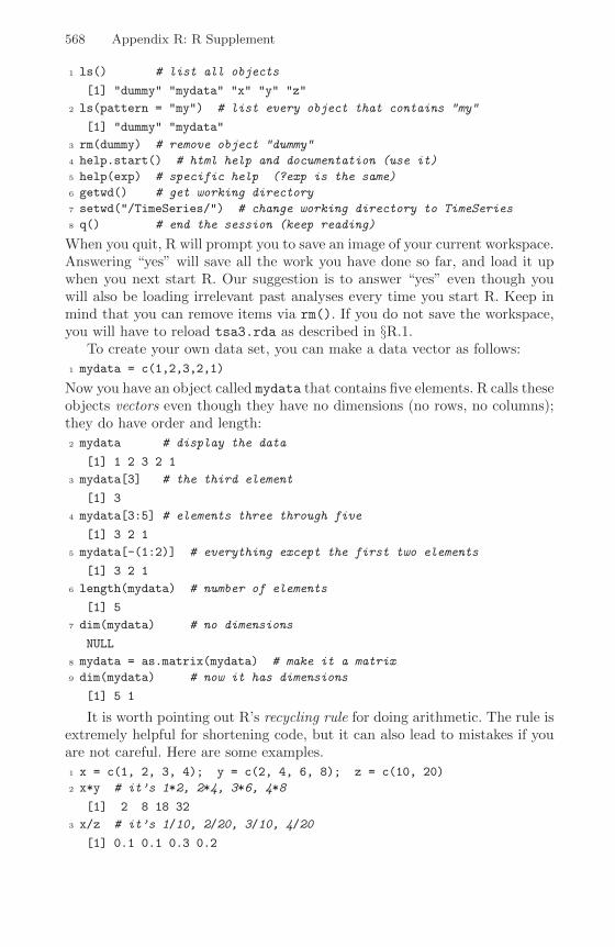
568 Appendix R: R Supplement
1 ls() # list all objects
[1] "dummy" "mydata" "x" "y" "z"
2 ls(pattern = "my") # list every object that contains "my"
[1] "dummy" "mydata"
3 rm(dummy) # remove object "dummy"
4 help.start() # html help and documentation (use it)
5 help(exp) # specific help (?exp is the same)
6 getwd() # get working directory
7 setwd("/TimeSeries/") # change working directory to TimeSeries
8 q() # end the session (keep reading)
When you quit, R will prompt you to save an image of your current workspace.Answering “yes” will save all the work you have done so far, and load it upwhen you next start R. Our suggestion is to answer “yes” even though youwill also be loading irrelevant past analyses every time you start R. Keep inmind that you can remove items via rm(). If you do not save the workspace,you will have to reload tsa3.rda as described in §R.1.
To create your own data set, you can make a data vector as follows:
1 mydata = c(1,2,3,2,1)
Now you have an object called mydata that contains five elements. R calls theseobjects vectors even though they have no dimensions (no rows, no columns);they do have order and length:
2 mydata # display the data
[1] 1 2 3 2 1
3 mydata[3] # the third element
[1] 3
4 mydata[3:5] # elements three through five
[1] 3 2 1
5 mydata[-(1:2)] # everything except the first two elements
[1] 3 2 1
6 length(mydata) # number of elements
[1] 5
7 dim(mydata) # no dimensions
NULL
8 mydata = as.matrix(mydata) # make it a matrix
9 dim(mydata) # now it has dimensions
[1] 5 1
It is worth pointing out R’s recycling rule for doing arithmetic. The rule isextremely helpful for shortening code, but it can also lead to mistakes if youare not careful. Here are some examples.
1 x = c(1, 2, 3, 4); y = c(2, 4, 6, 8); z = c(10, 20)
2 x*y # it’s 1*2, 2*4, 3*6, 4*8
[1] 2 8 18 32
3 x/z # it’s 1/10, 2/20, 3/10, 4/20
[1] 0.1 0.1 0.3 0.2

R.2 Getting Started 569
4 x+z # guess
[1] 11 22 13 24
If you have an external data set, you can use scan or read.table toinput the data. For example, suppose you have an ascii (text) data file calleddummy.dat in a directory called TimeSeries in your root directory, and thefile looks like this:
1 2 3 2 19 0 2 1 0
1 dummy = scan("dummy.dat") # if TimeSeries is the working directory
2 (dummy = scan("/TimeSeries/dummy.dat")) # if not, do this
Read 10 items
[1] 1 2 3 2 1 9 0 2 1 0
3 (dummy = read.table("/TimeSeries/dummy.dat"))
V1 V2 V3 V4 V5
1 2 3 2 1
9 0 2 1 0
There is a difference between scan and read.table. The former produced adata vector of 10 items while the latter produced a data frame with namesV1 to V5 and two observations per variate. In this case, if you want to list (oruse) the second variate, V2, you would use
4 dummy$V2
[1] 2 0
and so on. You might want to look at the help files ?scan and ?read.table
now. Data frames (?data.frame) are “used as the fundamental data structureby most of R’s modeling software.” Notice that R gave the columns of dummygeneric names, V1, ..., V5. You can provide your own names and then usethe names to access the data without the use of $ as in line 4 above.
5 colnames(dummy) = c("Dog", "Cat", "Rat", "Pig", "Man")
6 attach(dummy)
7 Cat
[1] 2 0
R is case sensitive, thus cat and Cat are different. Also, cat is a reservedname (?cat) in R, so using "cat" instead of "Cat" may cause problems later.You may also include a header in the data file to avoid using line 5 above;type ?read.table for further information.
It can’t hurt to learn a little about programming in R because you will seesome of it along the way. Consider a simple program that we will call crazyto produce a graph of a sequence of sample means of increasing sample sizesfrom a Cauchy distribution with location parameter zero. The code is:
1 crazy <- function(num) {
2 x <- rep(NA, num)
3 for (n in 1:num) x[n] <- mean(rcauchy(n))
4 plot(x, type="l", xlab="sample size", ylab="sample mean")
5 }

570 Appendix R: R Supplement
0 20 40 60 80 100
−40
−20
020
40
sample size
sam
ple
mea
n
Fig. R.1. Crazy example.
The first line creates the function crazy and gives it one argument, num, thatis the sample size that will end the sequence. Line 2 makes a vector, x, ofnum missing values NA, that will be used to store the sample means. Line 3generates n random Cauchy variates [rcauchy(n)], finds the mean of thosevalues, and puts the result into x[n], the n-th value of x. The process isrepeated in a “do loop” num times so that x[1] is the sample mean from asample of size one, x[2] is the sample mean from a sample of size two, and soon, until finally, x[num] is the sample mean from a sample of size num. Afterthe do loop is complete, the fourth line generates a graphic (see Figure R.1).The fifth line closes the function. To use crazy with a limit sample size of100, for example, type
6 crazy(100)
and you will get a graphic that looks like Figure R.1You may want to use one of the R packages. In this case you have to first
download the package and then install it. For example,
1 install.packages(c("wavethresh", "tseries"))
will download and install the packages wavethresh that we use in Chapter 4and tseries that we use in Chapter 5; you will be asked to choose the closestmirror to you. To use a package, you have to load it at each start up of R, forexample:
2 library(wavethresh) # load the wavethresh package
A good way to get help for a package is to use html help
3 help.start()
and follow the Packages link.Finally, a word of caution: TRUE and FALSE are reserved words, whereas T
and F are initially set to these. Get in the habit of using the words rather thanthe letters T or F because you may get into trouble if you do something likeF = qf(p=.01, df1=3, df2=9), so that F is no longer FALSE, but a quantileof the specified F -distribution.
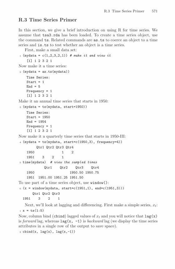
R.3 Time Series Primer 571
R.3 Time Series Primer
In this section, we give a brief introduction on using R for time series. Weassume that tsa3.rda has been loaded. To create a time series object, usethe command ts. Related commands are as.ts to coerce an object to a timeseries and is.ts to test whether an object is a time series.
First, make a small data set:
1 (mydata = c(1,2,3,2,1)) # make it and view it
[1] 1 2 3 2 1
Now make it a time series:
2 (mydata = as.ts(mydata))
Time Series:
Start = 1
End = 5
Frequency = 1
[1] 1 2 3 2 1
Make it an annual time series that starts in 1950:
3 (mydata = ts(mydata, start=1950))
Time Series:
Start = 1950
End = 1954
Frequency = 1
[1] 1 2 3 2 1
Now make it a quarterly time series that starts in 1950-III:
4 (mydata = ts(mydata, start=c(1950,3), frequency=4))
Qtr1 Qtr2 Qtr3 Qtr4
1950 1 2
1951 3 2 1
5 time(mydata) # view the sampled times
Qtr1 Qtr2 Qtr3 Qtr4
1950 1950.50 1950.75
1951 1951.00 1951.25 1951.50
To use part of a time series object, use window():
6 (x = window(mydata, start=c(1951,1), end=c(1951,3)))
Qtr1 Qtr2 Qtr3
1951 3 2 1
Next, we’ll look at lagging and differencing. First make a simple series, xt:
1 x = ts(1:5)
Now, column bind (cbind) lagged values of xt and you will notice that lag(x)is forward lag, whereas lag(x, -1) is backward lag (we display the time seriesattributes in a single row of the output to save space).
2 cbind(x, lag(x), lag(x,-1))

572 Appendix R: R Supplement
Time Series: Start = 0 End = 6 Frequency = 1
x lag(x) lag(x, -1)
0 NA 1 NA
1 1 2 NA
2 2 3 1
3 3 4 2 <- in this row, for example, x is 3,
4 4 5 3 lag(x) is ahead at 4, and
5 5 NA 4 lag(x,-1) is behind at 2
6 NA NA 5
Compare cbind and ts.intersect:
3 ts.intersect(x, lag(x,1), lag(x,-1))
Time Series: Start = 2 End = 4 Frequency = 1
x lag(x, 1) lag(x, -1)
2 2 3 1
3 3 4 2
4 4 5 3
To difference a series, ∇xt = xt − xt−1, use
1 diff(x)
but note that
2 diff(x, 2)
is not second order differencing, it is xt − xt−2. For second order differencing,that is, ∇2xt, do this:
3 diff(diff(x))
and so on for higher order differencing.
For graphing time series, there a few standard plotting mechanisms thatwe use repeatedly. If x is a time series, then plot(x) will produce a time plot.If x is not a time series object, then plot.ts(x) will coerce it into a time plotas will ts.plot(x). There are differences, which we explore in the following.It would be a good idea to skim the graphical parameters help file (?par)while you are here.2 See Figure R.2 for the resulting graphic.
1 x = -5:5 # x is NOT a time series object
2 y = 5*cos(x) # neither is y
3 op = par(mfrow=c(3,2)) # multifigure setup: 3 rows, 2 cols
4 plot(x, main="plot(x)")
5 plot(x, y, main="plot(x,y)")
6 plot.ts(x, main="plot.ts(x)")
7 plot.ts(x, y, main="plot.ts(x,y)")
8 ts.plot(x, main="ts.plot(x)")
9 ts.plot(ts(x), ts(y), col=1:2, main="ts.plot(x,y)")
10 par(op) # reset the graphics parameters [see footnote]
2 In the plot example, the parameter set up uses op = par(...) and ends withpar(op); these lines are used to reset the graphic parameters to their previoussettings. Please make a note of this because we do not display these commandsad nauseam in the text.
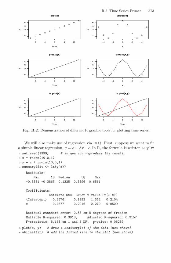
R.3 Time Series Primer 573
2 4 6 8 10
−40
24
plot(x)
Index
x
−4 −2 0 2 4
−40
24
plot(x,y)
x
y
plot.ts(x)
Time
x
2 4 6 8 10
−40
24
−4 −2 0 2 4
−40
24
plot.ts(x,y)
xy
1
2
3
4
5
6
7
8
9
10
11
ts.plot(x)
Time
x
2 4 6 8 10
−40
24
ts.plot(x,y)
Time
2 4 6 8 10
−40
24
Fig. R.2. Demonstration of different R graphic tools for plotting time series.
We will also make use of regression via lm(). First, suppose we want to fita simple linear regression, y = α+βx+ ε. In R, the formula is written as y~x:
1 set.seed(1999) # so you can reproduce the result
2 x = rnorm(10,0,1)
3 y = x + rnorm(10,0,1)
4 summary(fit <- lm(y~x))
Residuals:
Min 1Q Median 3Q Max
-0.8851 -0.3867 0.1325 0.3896 0.6561
Coefficients:
Estimate Std. Error t value Pr(>|t|)
(Intercept) 0.2576 0.1892 1.362 0.2104
x 0.4577 0.2016 2.270 0.0529
Residual standard error: 0.58 on 8 degrees of freedom
Multiple R-squared: 0.3918, Adjusted R-squared: 0.3157
F-statistic: 5.153 on 1 and 8 DF, p-value: 0.05289
5 plot(x, y) # draw a scatterplot of the data (not shown)
6 abline(fit) # add the fitted line to the plot (not shown)

574 Appendix R: R Supplement
All sorts of information can be extracted from the lm object, which we calledfit. For example,
7 resid(fit) # will display the residuals (not shown)
8 fitted(fit) # will display the fitted values (not shown)
9 lm(y ~ 0 + x) # will exclude the intercept (not shown)
You have to be careful if you use lm() for lagged values of a time se-ries. If you use lm(), then what you have to do is “tie” the series togetherusing ts.intersect. If you do not tie the series together, they will not bealigned properly. Please read the warning Using time series in the lm() helpfile [help(lm)]. Here is an example regressing Chapter 2 data, weekly car-diovascular mortality (cmort) on particulate pollution (part) at the presentvalue and lagged four weeks (part4). First, we create a data frame called ded
that consists of the three series:
1 ded = ts.intersect(cmort, part, part4=lag(part,-4), dframe=TRUE)
Now the series are all aligned and the regression will work.
2 fit = lm(mort~part+part4, data=ded, na.action=NULL)
3 summary(fit)
Call: lm(formula=mort~part+part4,data=ded,na.action=NULL)
Residuals:
Min 1Q Median 3Q Max
-22.7429 -5.3677 -0.4136 5.2694 37.8539
Coefficients:
Estimate Std. Error t value Pr(>|t|)
(Intercept) 69.01020 1.37498 50.190 < 2e-16
part 0.15140 0.02898 5.225 2.56e-07
part4 0.26297 0.02899 9.071 < 2e-16
Residual standard error: 8.323 on 501 degrees of freedom
Multiple R-Squared: 0.3091, Adjusted R-squared: 0.3063
F-statistic: 112.1 on 2 and 501 DF, p-value: < 2.2e-16
There was no need to rename lag(part,-4) to part4, it’s just an exampleof what you can do. There is a package called dynlm that makes it easy to fitlagged regressions. The basic advantage of dynlm is that it avoids having tomake a data frame; that is, line 1 would be avoided.
In Problem 2.1, you are asked to fit a regression model
xt = βt+ α1Q1(t) + α2Q2(t) + α3Q3(t) + α4Q4(t) + wt
where xt is logged Johnson & Johnson quarterly earnings (n = 84), and Qi(t)is the indicator of quarter i = 1, 2, 3, 4. The indicators can be made usingfactor.
1 trend = time(jj) - 1970 # helps to ‘center’ time
2 Q = factor(rep(1:4, 21)) # make (Q)uarter factors
3 reg = lm(log(jj)~0 + trend + Q, na.action=NULL) # no intercept
4 model.matrix(reg) # view the model matrix
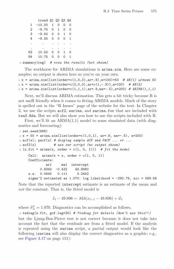
R.3 Time Series Primer 575
trend Q1 Q2 Q3 Q4
1 -10.00 1 0 0 0
2 -9.75 0 1 0 0
3 -9.50 0 0 1 0
4 -9.25 0 0 0 1
. . . . . .
. . . . . .
83 10.50 0 0 1 0
84 10.75 0 0 0 1
5 summary(reg) # view the results (not shown)
The workhorse for ARIMA simulations is arima.sim. Here are some ex-amples; no output is shown here so you’re on your own.
1 x = arima.sim(list(order=c(1,0,0),ar=.9),n=100)+50 # AR(1) w/mean 50
2 x = arima.sim(list(order=c(2,0,0),ar=c(1,-.9)),n=100) # AR(2)
3 x = arima.sim(list(order=c(1,1,1),ar=.9,ma=-.5),n=200) # ARIMA(1,1,1)
Next, we’ll discuss ARIMA estimation. This gets a bit tricky because R isnot useR friendly when it comes to fitting ARIMA models. Much of the storyis spelled out in the “R Issues” page of the website for the text. In Chapter3, we use the scripts acf2, sarima, and sarima.for that are included withtsa3.Rda. But we will also show you how to use the scripts included with R.
First, we’ll fit an ARMA(1,1) model to some simulated data (with diag-nostics and forecasting):
1 set.seed(666)
2 x = 50 + arima.sim(list(order=c(1,0,1), ar=.9, ma=-.5), n=200)
3 acf(x); pacf(x) # display sample ACF and PACF ... or ...
4 acf2(x) # use our script (no output shown)
5 (x.fit = arima(x, order = c(1, 0, 1))) # fit the model
Call: arima(x = x, order = c(1, 0, 1))
Coefficients:
ar1 ma1 intercept
0.8340 -0.432 49.8960
s.e. 0.0645 0.111 0.2452
sigma^2 estimated as 1.070: log likelihood = -290.79, aic = 589.58
Note that the reported intercept estimate is an estimate of the mean andnot the constant. That is, the fitted model is
xt − 49.896 = .834(xt−1 − 49.896) + wt
where σ2w = 1.070. Diagnostics can be accomplished as follows,
4 tsdiag(x.fit, gof.lag=20) # ?tsdiag for details (don’t use this!!)
but the Ljung-Box-Pierce test is not correct because it does not take intoaccount the fact that the residuals are from a fitted model. If the analysisis repeated using the sarima script, a partial output would look like thefollowing (sarima will also display the correct diagnostics as a graphic; e.g.,see Figure 3.17 on page 151):

576 Appendix R: R Supplement
1 sarima(x, 1, 0, 1)
Coefficients:
ar1 ma1 xmean
0.8340 -0.432 49.8960
s.e. 0.0645 0.111 0.2452
sigma^2 estimated as 1.070: log likelihood = -290.79, aic = 589.58
$AIC [1] 1.097494 $AICc [1] 1.108519 $BIC [1] 0.1469684
Finally, to obtain and plot the forecasts, you can use the following R code:
1 x.fore = predict(x.fit, n.ahead=10)
2 U = x.fore$pred + 2*x.fore$se # x.fore$pred holds predicted values
3 L = x.fore$pred - 2*x.fore$se # x.fore$se holds stnd errors
4 miny = min(x,L); maxy = max(x,U)
5 ts.plot(x, x.fore$pred, col=1:2, ylim=c(miny, maxy))
6 lines(U, col="blue", lty="dashed")
7 lines(L, col="blue", lty="dashed")
Using the script sarima.for, you can accomplish the same task in one line.
1 sarima.for(x, 10, 1, 0, 1)
Example 3.46 on page 159 uses this script.We close this appendix with a quick spectral analysis. This material is
covered in detail in Chapter 4, so we will not discuss this example in muchdetail here. We will simulate an AR(2) and then estimate the spectrum vianonparametric and parametric methods. No graphics are shown, but we haveconfidence that you are proficient enough in R to display them yourself.
1 x = arima.sim(list(order=c(2,0,0), ar=c(1,-.9)), n=2^8) # some data
2 (u = polyroot(c(1,-1,.9))) # x is AR(2) w/complex roots
[1] 0.5555556+0.8958064i 0.5555556-0.8958064i
3 Arg(u[1])/(2*pi) # dominant frequency around .16
[1] 0.1616497
4 par(mfcol=c(4,1))
5 plot.ts(x)
6 spec.pgram(x,spans=c(3,3),log="no") # nonparametric spectral estimate
7 spec.ar(x, log="no") # parametric spectral estimate
8 spec.arma(ar=c(1,-.9), log="no") # true spectral density
The script spec.arma is included in tsa3.rda. Also, see spectrum as analternative to spec.pgram. Finally, note that R tapers and logs by default, so ifyou simply want the periodogram of a series, the command is spec.pgram(x,taper=0, fast=FALSE, detrend=FALSE, log="no"). If you just asked forspec.pgram(x), you would not get the raw periodogram because the dataare detrended, possibly padded, and tapered, even though the title of theresulting graphic would say Raw Periodogram. An easier way to get a rawperiodogram is:
9 per = abs(fft(x))^2/length(x)
This final example points out the importance of knowing the defaults for theR scripts you use.