TIME-SCALES OF THE VARIABILITY OF THE ATMOSPHERE

INTERNATIONAL JOURNAL OF CLIMATOLOGY, VOL. 16,499-535 (1996)

TIME-SCALES OF THE VARIABILITY OF THE ATMOSPHERE

ANTHONY G . BARNSTON Climate Prediction Center, NCEPINWSINOAA, Washington. DC 20233, USA

Received 16 December 1994 Accepted 7 August 1995

ABSTRACT

In this study the time-scales of variability of several weather elements are explored by season and location across the globe, emphasizing the Northern Hemisphere and especially the USA. The resulting description is useful because regions that exhibit low frequency variability (i.e. longer periods than the 2-5 days synoptic-scale) are assumed to be related more directly to changes in boundary conditions (e.g. anomalies of ENSO-related sea-surface temperature [SST], snow cover, etc.). Therefore, this low frequency variability may be predictable at greater ranges than those for which numerical weather prediction is helpful.

New as well as established measures of persistence and frequency dependence are used and intercompared. In particular, the standard deviation of the differences between adjacent period means, when compared over a range of period lengths, reflects both autocorrelation and (if applicable) cycle time. Frequency dependence is thereby summarized with minimal computation.

The geographical distribution of the amplitude (amount of variability depends largely on latitude and the upstream geographical environment (i.e. higher latitude and continentality of upstream environment tend to increase variability). At most locations, variability is greatest (lowest) during the cold (warm) seasons of the year. The geographical distribution of the dominant frequencies of variability are examined by season for Northern Hemisphere sea-level pressure and 700 hPa geopotential height, and USA surface temperature and precipitation. It is demonstrated that the dominant frequencies tend to vary in parallel across all four fields.

In general, weather variables are found to vary at relatively low frequency (long periods) at high latitudes and, to a lesser extent, at subtropical latitudes. At mid-latitude, low frequency Variability prevails most over the blocking regions in the eastern and central North Pacific and North Atlantic oceans. High frequency variability occurs in the synoptically active jet exit regions over the western oceans and the eastern and central parts of the Northern Hemisphere continents.

Data from the Atmospheric Model Intercomparison Project integration of the National Centers for Environmental Prediction (formerly National Meteorological Center) medium-range-forecast general circulation model, which reproduce the Northern Hemisphere frequency dependence well at 700 hPa, indicate roughly analogous behaviour in the Southern Hemisphere. However, the longitudinal variation of mid-latitude frequency dependence is substantially less in the Southern Hemisphere, possibly because of the comparative absence of large, topographically significant land masses with favourable separation distance.

KEY WORDS: USA; Northem Hemisphere; fast Fourier transform; autocorrelation; temporal variability scales; empirical modelling of variability; surface temperatures; 700 hPa height.

1. INTRODUCTION

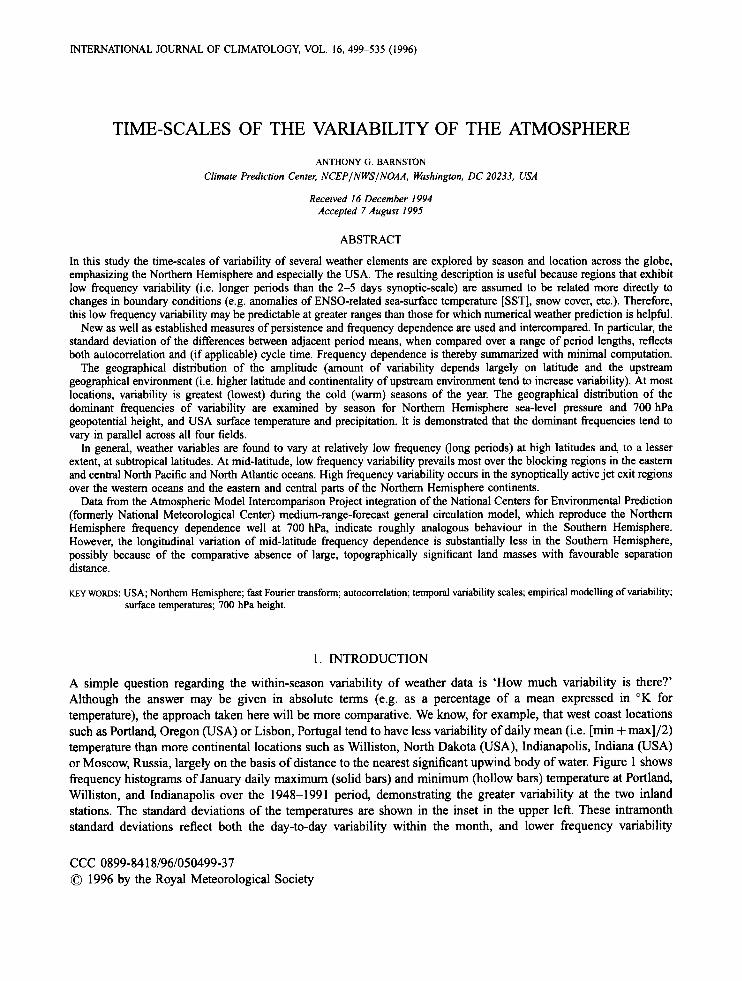
A simple question regarding the within-season variability of weather data is ‘How much variability is there?’ Although the answer may be given in absolute terms (e.g. as a percentage of a mean expressed in OK for temperature), the approach taken here will be more comparative. We know, for example, that west coast locations such as Portland, Oregon (USA) or Lisbon, Portugal tend to have less variability of daily mean (i.e. [min + max]/2) temperature than more continental locations such as Williston, North Dakota (USA), Indianapolis, Indiana (USA) or Moscow, Russia, largely on the basis of distance to the nearest significant upwind body of water. Figure 1 shows frequency histograms of January daily maximum (solid bars) and minimum (hollow bars) temperature at Portland, Williston, and Indianapolis over the 1948-1991 period, demonstrating the greater variability at the two inland stations. The standard deviations of the temperatures are shown in the inset in the upper left. These intramonth standard deviations reflect both the day-to-day variability within the month, and lower frequency variability

CCC 0899-841 8/96/050499-3 7 0 1996 by the Royal Meteorological Society

500 A. G . BARNSTON

persumably related to changing boundary conditions-a major contributor to year-to-year mean differences. A third, perhaps undesired, contribution to the standard deviations is the gradual seasonal change in mean temperature within the month. In a climatological sense, this factor matters most during spring and autumn, and is negligible in mid-winter and mid-summer.

The day-to-day variability of temperature can also be expressed by the interannual standard deviation of temperature for a given day of the year, or for a composite of a small group of such individual days spanning adjacent dates. This approach would eliminate the gradual seasonal change as a contributor to the interdiumal standard deviation.

The interannual standard deviation of monthly mean temperature has been compiled in technical reports such as Shea (1984) or May et al. (1 992). This standard deviation is smaller than that for daily tempratures, with the factor of decrease depending on the day-to-day autocorrelation: the less the autocorrelation, the greater the factor. Because the autocorrelation varies with location, the monthly mean standard deviation field cannot be used as an accurate indicator of the field of interannual standard deviation of daily temperatures.

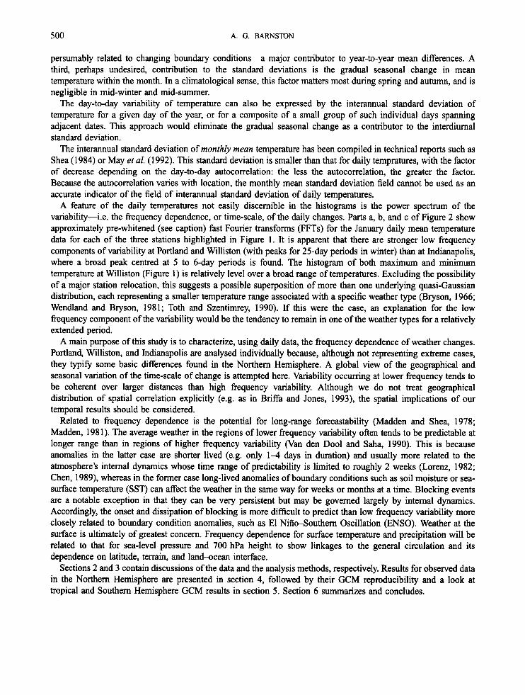
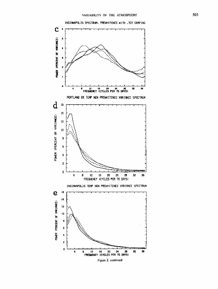
A feature of the daily temperatures not easily discernible in the histograms is the power spectrum of the variability-i.e. the frequency dependence, or time-scale, of the daily changes. Parts a, b, and c of Figure 2 show approximately pre-whitened (see caption) fast Fourier transforms (FFTs) for the January daily mean temperature data for each of the three stations highlighted in Figure 1. It is apparent that there are stronger low frequency components of variability at Portland and Williston (with peaks for 25-day periods in winter) than at Indianapolis, where a broad peak centred at 5 to 6-day periods is found. The histogram of both maximum and minimum temperature at Williston (Figure 1) is relatively level over a broad range of temperatures. Excluding the possibility of a major station relocation, this suggests a possible superposition of more than one underlying quasi-Gaussian distribution, each representing a smaller temperature range associated with a specific weather type (Bryson, 1966; Wendland and Bryson, 1981; Toth and Szentimrey, 1990). If this were the case, an explanation for the low frequency component of the variability would be the tendency to remain in one of the weather types for a relatively extended period.

A main purpose of this study is to characterize, using daily data, the frequency dependence of weather changes. Portland, Williston, and Indianapolis are analysed individually because, although not representing extreme cases, they typify some basic differences found in the Northern Hemisphere. A global view of the geographical and seasonal variation of the time-scale of change is attempted here. Variability occurring at lower frequency tends to be coherent over larger distances than high frequency variability. Although we do not treat geographical distribution of spatial correlation explicitly (e.g. as in Briffa and Jones, 1993), the spatial implications of our temporal results should be considered.

Related to frequency dependence is the potential for long-range forecastability (Madden and Shea, 1978; Madden, 1981). The average weather in the regions of lower frequency variability often tends to be predictable at longer range than in regions of higher frequency variability (Van den Do01 and Saha, 1990). This is because anomalies in the latter case are shorter lived (e.g. only 1 4 days in duration) and usually more related to the atmosphere’s internal dynamics whose time range of predictability is limited to roughly 2 weeks (Lorenz, 1982; Chen, 1989), whereas in the former case long-lived anomalies of boundary conditions such as soil moisture or sea- surface temperature (SST) can affect the weather in the same way for weeks or months at a time. Blocking events are a notable exception in that they can be very persistent but may be governed largely by internal dynamics. Accordingly, the onset and dissipation of blocking is more difficult to predict than low frequency variability more closely related to boundary condition anomalies, such as El Niiio-Southern Oscillation (ENSO). Weather at the surface is ultimately of greatest concern. Frequency dependence for surface temperature and precipitation will be related to that for sea-level pressure and 700 hPa height to show linkages to the general circulation and its dependence on latitude, terrain, and land-ocean interface.

Sections 2 and 3 contain discussions of the data and the analysis methods, respectively. Results for observed data in the Northern Hemisphere are presented in section 4, followed by their GCM reproducibility and a look at tropical and Southern Hemisphere GCM results in section 5 . Section 6 summarizes and concludes.

VARIABILITY OF THE ATMOSPHERE

P O R T L f l N D O R

50 1

JRNURRY 0 tn

0 3

0 (u

0

- R Y C Y C 1 ~ ~ I ~ 2 ~ Z ~ Z I Z D I ~ l ~ l l - B -6 -2 1 Y I I0 11 II I 0 22 26 Z# 81 MI 17 Y O U 1 YE Y 1 51 66

TEMPERATURE INTERVAL (C)

WILLISTON NO JRNURRY

0 w a L O I * 0

d I2 I5 In 21 26 27 30 33 36 39 YI Y Y u7 50 51 so

INDIRNAPOLIS IN

TEMPERATURE INTERVAL I C I

Figure 1. Frequency histograms of January daily temperature over the 1948-1991 period at three US,4 stations: (a) Portland, Oregon, (b) Williston, North Dakota, and (c) Indianapolis, Indiana. Daily maximum temperature frequencies are indicated by solid bars, and daily minimum by hollow bars. Very short but non-zero (i.e. less than one-half per cent) bars are highlighted by crosses (for maximum temperature) or pairs of dots (for minimum). Some summary statistics for the maximum and minimum temperatures are shown in the upper left, and the SDA

and l-day autocorrelation for daily mean temperatures (see sections 2b and 4% respectively) are shown in the upper right

502 A. G. BARNSTON

PORTLAND, OR SPECTRUM. PREWHITENED WITH -707 DAMPING

c 4

b

8 a 1

0 4 8 1 2 1 6 2 O W z B U 3 6

FREQUENCY (CYCLES PER 75 DRYS1

WILLISTON SPECTRUM. PREWHITENEO WITH -707 DAMPING

b

t 1 4 8 I t 1 6 2 0 2 4 2 0 3 2 3 6

FREWENCY (CYCLES PER 75 DRYS1

Figure 2. Fast Fourier transform (FFT) of daily mean temperature over the 1948-1991 period at Portland, Williston, and Indianapolis (see Figure 1) during 75-day periods in each of the four seasons. The 75-day segment for each year was tapered, and the squared Fourier coefficients were averaged over all years. The solid curve represents winter (15 December to 29 February), the small dashed curve spring, medium dashed curve summer, and large dashed curve autumn. In parts (a), (b), and (c) the spectrum is approximately pre-whitened by using the change between the previous day’s temperature multiplied by 0.707 and the present day’s temperature; in parts (d) and (e) no pre-whitening is done. The constant 0.707 is used to produce a roughly ‘level’ FFT curve. The noisy ‘raw’solutions have been smoothed with a five-point Gaussian moving average

VARIABILITY OF THE ATMOSPHERE 503

INDIWAPOLIS SPECTRUM. PREWHITENED WITH .707 DAMPING

b

~ 8 I Z I 6 2 0 2 4 2 8 ~ 3 6 FRE:WENCY (CYUES PER 75 DRTS)

PORTLAND OR TEMP NON PREWHITENED VRRIANCE SPECTRUM

- W x #-I

K > a LL 0 I- z W u K W &

14

12

10

8

6

K

0 L Y q

2

[I

4 8 12 16 M 24 28 32 36 FREQUENCY ICYCLES PER 75 DAYS1

INDIRNWOLIS TEMP NON PREWHITENED VRRIRNCE SPECTRUM

e l6 fi'

ki

I4

12

10

8

6

4

2

n '1 8 12 16 M 24 28 32 36

Figure 2. continued

FREQUENCY (CYCLES PER 75 OAYS)

504

6C

61

41

ai

21

k& + + + + +

/ + +

A. G. BARNSTON

6UN

SON

40N

'aON

20N

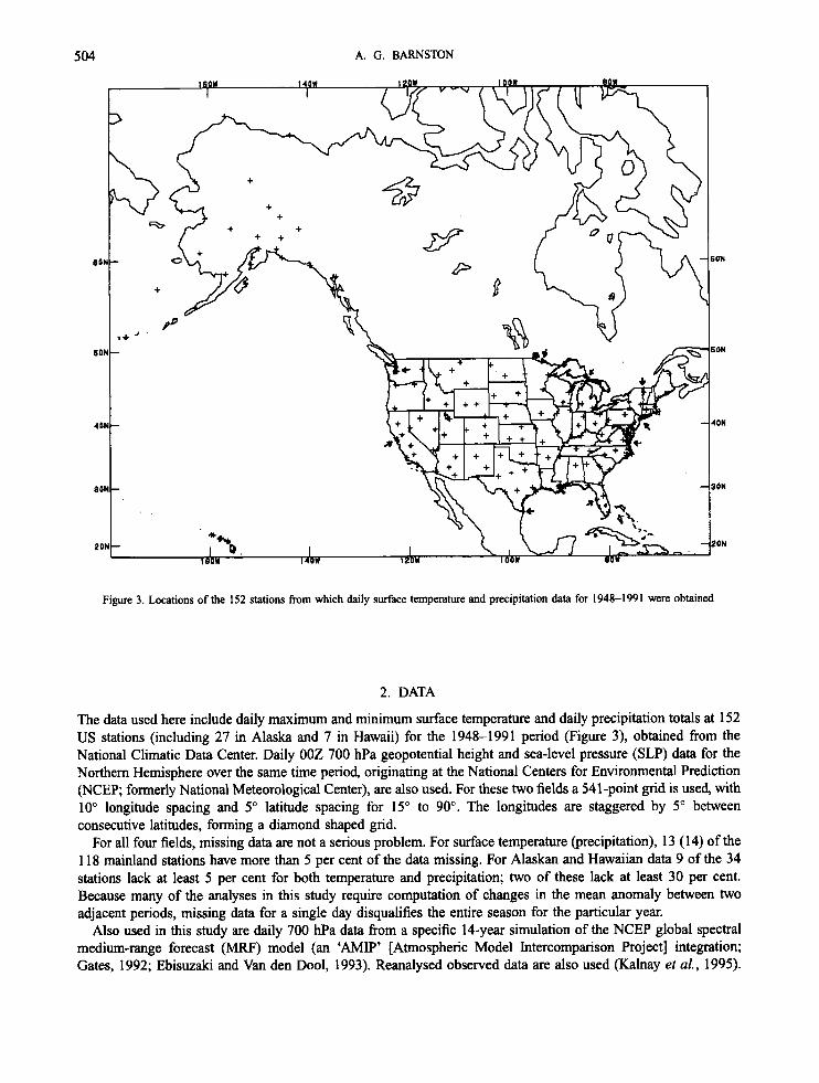
Figure 3. Locations of the 152 stations from which daily surface temperature and precipitation data for 1948-1991 were obtained

2. DATA

The data used here include daily maximum and minimum surface temperature and daily precipitation totals at 152 US stations (including 27 in Alaska and 7 in Hawaii) for the 1948-1991 period (Figure 3), obtained from the National Climatic Data Center. Daily OOZ 700 hPa geopotential height and sea-level pressure (SLP) data for the Northern Hemisphere over the same time period, originating at the National Centers for Environmental Prediction (NCEP; formerly National Meteorological Center), are also used. For these two fields a 541-point grid is used, with 10" longitude spacing and 5" latitude spacing for 15" to 90". The longitudes are staggered by 5" between consecutive latitudes, forming a diamond shaped grid.

For all four fields, missing data are not a serious problem. For surface temperature (precipitation), 13 (14) of the 118 mainland stations have more than 5 per cent of the data missing. For Alaskan and Hawaiian data 9 of the 34 stations lack at least 5 per cent for both temperature and precipitation; two of these lack at least 30 per cent. Because many of the analyses in this study require computation of changes in the mean anomaly between two adjacent periods, missing data for a single day disqualifies the entire season for the particular year.

Also used in this study are daily 700 hPa data from a specific 14-year simulation of the NCEP global spectral medium-range forecast (MRF) model (an 'AMIP' [Atmospheric Model Intercomparison Project] integration; Gates, 1992; Ebisuzaki and Van den Dool, 1993). Reanalysed observed data are also used (Kalnay et al., 1995).


3. METHODS

3. I . Established techniques

The FFT (Figure 2), representing an established method of describing frequency dependence in a time series, allows for as detailed a description as possible given the sampling frequency and the length of the time series. Figure 2 shows a stronger low frequency component of winter temperature variation in Portland (peaking at three cycles per 75 days) than at Williston, and relatively the smallest component at that frequency at Indianapolis. Because there is marked persistence (or ‘redness’) in all surface temperature data, approximate ‘pre-whitening’ has been applied to parts a, b, and c of Figure 2. To illustrate the greater difficulty in distinguishing FFT differences in the naturally red FFT results, parts d and e show those of Portland and Indianapolis without pre-whitening. The amounts of power at middle frequency (e.g. the 4 5 day period) are more difficult to compare in the non-prewhitened results.

Another way to identify the dominant frequencies in broader terms is by filtering the original data one or more times, preserving specific frequency ranges in each case, and then calculating ratios of the resulting variances to the original total or to one another. This was one aspect of the approach of Blackmon (1976) and Blaclanon and Lee (1984a,b) in identifjhg the regions and/or seasons of low versus high frequency variability in Northern Hemisphere geopotential height. Because variances were computed over the span of years of record for a given time of year, interannual variability (in the sense of changes in the overall mean from year to year) is one of the components in these studies’ results.

Measurement of variability of adjacent period data within a defined seasonal window of each year individually, and then compositing results over all years, is another approach to the description of frequency dependence, and the one used here. This approach has the feature of omitting variation in the mean from year to year-either unexplained or related to climate regimes or trends. These are omitted because each year’s mean is implicitly removed in the analysis of individual year variability. Thus, the frequencies described are no longer than the seasonal window itself. This is seen as an advantage here, because resolution of variations on synoptic to short- term climate time-scales is intended.

3.2. The standard deviation of adjacent period change

3.2.1. Dejinition and computation. The statistic developed here to express frequency dependence in a time series is the standard deviation of adjacent period change (SDA), using periods of a selected number of days (N). Using the adjacent period data within a fixed seasonal window, the effects of the seasonal march are removed from SDA by initially subtracting a smoothed daily climatology. The curve of SDA as a fimction of N has a simple, intuitively clear meaning (described below). Although this application of SDA is not found in the literature, a version using a constant N of 1 day appears in Saha (1 992). Use of the change from period t to t + 1 eliminates interannual variability because each year’s overall mean is removed by using only the changes between adjacent periods within 1 year. The use of as many years as possible minimizes sampling uncertainty in SDA estimation. In computing the standard deviation of changes here, periods of length N days spanning 75 day ‘seasons’ are phased in each of the N possible ways in order to sample all possible phasings of the adjacent periods. For example, for ‘winter’ (1 6 December to 29 February), the standard deviation of changes of consecutive 4-day means ( N = 4) is computed with four phasings: that with the first period starting 16, 17, 18, and 19 December.

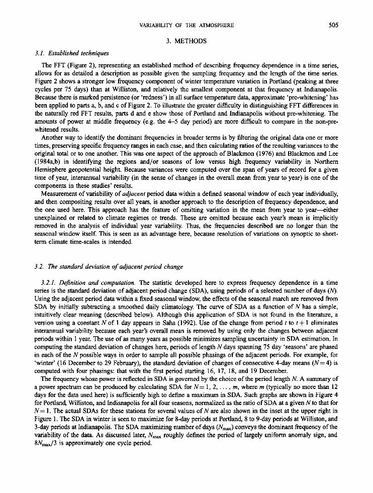
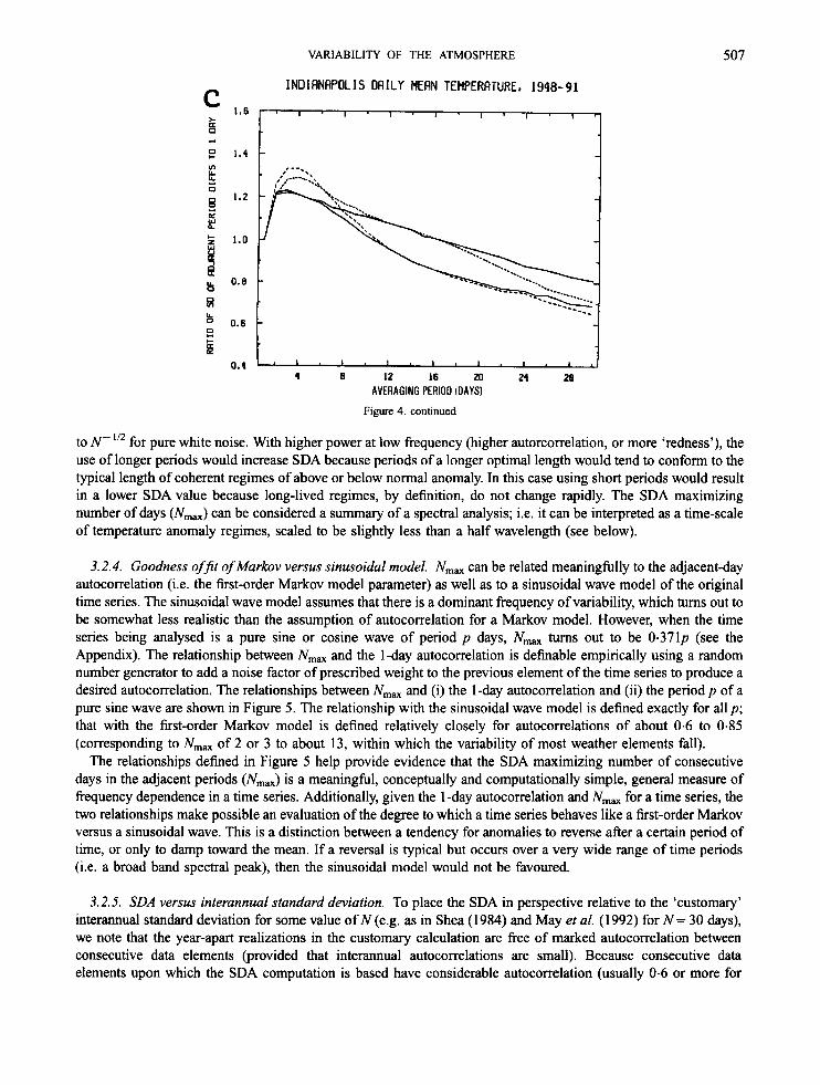
The frequency whose power is reflected in SDA is governed by the choice of the period length N. A summary of a power spectrum can be produced by calculating SDA for N = 1, 2, . . . , m, where m (typically no more than 12 days for the data used here) is sufficiently high to define a maximum in SDA. Such graphs are shown in Figure 4 for Portland, Williston, and Indianapolis for all four seasons, normalized as the ratio of SDA at a given N to that for N = 1. The actual SDAs for these stations for several values of N are also shown in the inset at the upper right in Figure 1. The SDA in winter is seen to maximize for 8-day periods at Portland, 8 to 9-day periods at Williston, and 3-day periods at Indianapolis. The SDA maximizing number of days (N-) conveys the dominant frequency of the variability of the data. As discussed later, N,, roughly defines the period of largely uniform anomaly sign, and 8N-13 is approximately one cycle period.

506 A. G. BARNSTON

PORTLAND, OR DAILY MEW TEMPERATURE. 1948-91

1.6 a li

b

!4 0

8 H

0.4

1.6

I , ¶

1.2

1.0

0.8

0.6

O.¶

I- 4

t I . I . I . I . I . I . I , I .J

RVERRCINC PERIOD (WYSI 4 8 12 16 20 21 28

WILLISTON DAILY MEAN TEHPERFITURE, 1948-91

4 8 12 16 20 2¶ 28 FIVERKING PERIOD (OAYSI

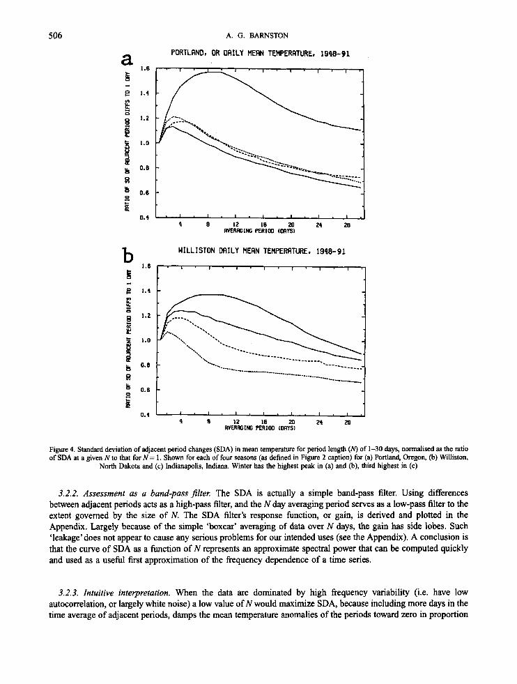
Figure 4. Standard deviation of adjacent period changes (SDA) in mean temperature for period length (N) of 1-30 days, normalised as the ratio of SDA at a given N to that for N = 1. Shown for each of four seasons (as defined in Figure 2 caption) for (a) Portland, Oregon, (b) Williston,

North Dakota and (c) Indianapolis, Indiana. Winter has the highest peak in (a) and (b), third highest in (c)

3.2.2. Assessment as a band-passfiltel: The SDA is actually a simple band-pass filter. Using differences between adjacent periods acts as a high-pass filter, and the N day averaging period serves as a low-pass filter to the extent governed by the size of N. The SDA filter’s response function, or gain, is derived and plotted in the Appendix. Largely because of the simple ‘boxcar’ averaging of data over N days, the gain has side lobes. Such ‘leakage’does not appear to cause any serious problems for our intended uses (see the Appendix). A conclusion is that the curve of SDA as a function of N represents an approximate spectral power that can be computed quickly and used as a usehl first approximation of the frequency dependence of a time series.

3.2.3. Intuitive interpretation. When the data are dominated by high frequency variability (i.e. have low autocorrelation, or largely white noise) a low value of N would maximize SDA, because including more days in the time average of adjacent periods, damps the mean temperature anomalies of the periods toward zero in proportion


INDIANAPOLIS DAILY MEAN TEMPERATURE, 1948-91

a

E LL

0.6

ii 0.4

I l . I . I , l . l . l . l .

4 8 I2 16 20 24 26 AVERAGING PERIOD (DAYS1

Figure 4. continued

With higher power at low frequency (higher autorcorrelation, or more ‘redness’), the to N - ”* for pure white noise. use of longer periods would increase SDA because periods of a longer optimal length would tend to conform to the typical length of coherent regimes of above or below normal anomaly. In this case using short periods would result in a lower SDA value because long-lived regimes, by definition, do not change rapidly. The SDA maximizing number of days (N,,) can be considered a summary of a spectral analysis; i.e. it can be interpreted as a time-scale of temperature anomaly regimes, scaled to be slightly less than a half wavelength (see below).

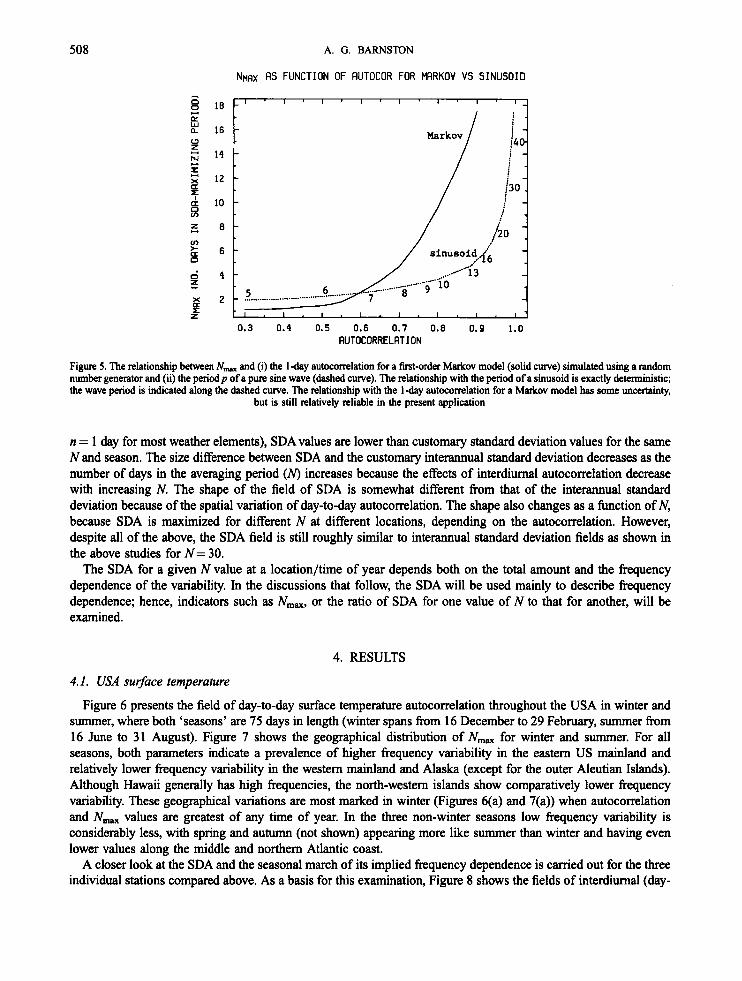
3.2.4. Goodness offit of Markov versus sinusoidal model. NmaX can be related meaningfully to the adjacent-day autocorrelation (i.e. the first-order Markov model parameter) as well as to a sinusoidal wave model of the original time series. The sinusoidal wave model assumes that there is a dominant frequency of variability, which turns out to be somewhat less realistic than the assumption of autocorrelation for a Markov model. However, when the time series being analysed is a pure sine or cosine wave of period p days, N,, tums out to be 0 . 3 7 1 ~ (see the Appendix). The relationship between N,, and the l-day autocorrelation is definable empirically using a random number generator to add a noise factor of prescribed weight to the previous element of the time series to produce a desired autocorrelation. The relationships between N,, and (i) the l-day autocorrelation and (ii) the periodp of a pure sine wave are shown in Figure 5. The relationship with the sinusoidal wave model is defined exactly for all p; that with the first-order Markov model is defined relatively closely for autocorrelations of about 0.6 to 0.85 (corresponding to N,, of 2 or 3 to about 13, within which the variability of most weather elements fall).

The relationships defined in Figure 5 help provide evidence that the SDA maximizing number of consecutive days in the adjacent periods (NmaX) is a meaningful, conceptually and computationally simple, general measure of frequency dependence in a time series. Additionally, given the l-day autocorrelation and N,,,, for a time series, the two relationships make possible an evaluation of the degree to which a time series behaves like a first-order Markov versus a sinusoidal wave. This is a distinction between a tendency for anomalies to reverse after a certain period of time, or only to damp toward the mean. If a reversal is typical but occurs over a very wide range of time periods (i.e. a broad band spectral peak), then the sinusoidal model would not be favoured.

3.2.5. SDA versus interannual standard deviation. To place the SDA in perspective relative to the ‘customary’ interannual standard deviation for some value of N (e.g. as in Shea (1 984) and May et al. (1 992) for N = 30 days), we note that the year-apart realizations in the customary calculation are free of marked autocorrelation between consecutive data elements (provided that interannual autocorrelations are small). Because consecutive data elements upon which the SDA computation is based have considerable autocorrelation (usually 0.6 or more for

508 A. G . BARNSTON

NMRX AS FUNCTION OF RUTOCOR FOR MRRKOV VS SINUSOID

- w W L 16

14

12

10

8

6

4

2

0.3 0.4 0.5 0.6 0.7 0.8 0.9 1.0 RUTOCORRELATION

Figure 5. The relationship between N- and (i) the 1-day autocorrelation for a first-order Markov model (solid curve) simulated using a random number generator and (ii) the periodp of a pure sine wave (dashed curve). The relationship with the period of a sinusoid is exactly deterministic; the wave period is indicated along the dashed curve. The relationship with the l-day autocorrelation for a Markov model has some uncertainty,

but is still relatively reliable in the present application

n = 1 day for most weather elements), SDA values are lower than customary standard deviation values for the same Nand season. The size difference between SDA and the customary interannual standard deviation decreases as the number of days in the averaging period (A‘) increases because the effects of interdiurnal autocorrelation decrease with increasing N. The shape of the field of SDA is somewhat different from that of the interannual standard deviation because of the spatial variation of day-to-day autocorrelation. The shape also changes as a h c t i o n of N, because SDA is maximized for different N at different locations, depending on the autocornlation. However, despite all of the above, the SDA field is still roughly similar to interannual standard deviation fields as shown in the above studies for N = 30.

The SDA for a given N value at a location/time of year depends both on the total amount and the frequency dependence of the variability. In the discussions that follow, the SDA will be used mainly to describe frequency dependence; hence, indicators such as N-, or the ratio of SDA for one value of N to that for another, will be examined.

4. RESULTS

4.1. USA surface temperature

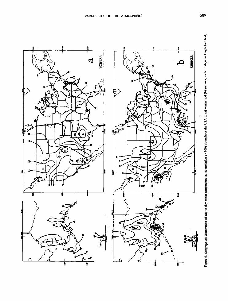
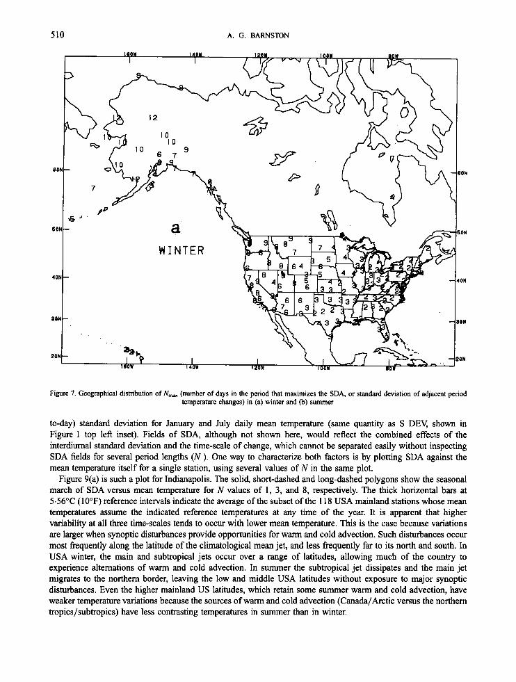
Figure 6 presents the field of day-to-day surface temperature autocorrelation throughout the USA in winter and summer, where both ‘seasons’ are 75 days in length (winter spans from 16 December to 29 February, summer from 16 June to 31 August). Figure 7 shows the geographical distribution of N- for winter and summer. For all seasons, both parameters indicate a prevalence of higher frequency variability in the eastern US mainland and relatively lower frequency variability in the western mainland and Alaska (except for the outer Aleutian Islands). Although Hawaii generally has high frequencies, the north-westem islands show comparatively lower frequency variability. These geographical variations are most marked in winter (Figures 6(a) and 7(a)) when autocorrelation and N,, values are greatest of any time of year. In the three non-winter seasons low fiequency variability is considerably less, with spring and autumn (not shown) appearing more like summer than winter and having even lower values along the middle and northern Atlantic coast.

A closer look at the SDA and the seasonal march of its implied frequency dependence is carried out for the three individual stations compared above. As a basis for this examination, Figure 8 shows the fields of interdiurnal (day-


L :: L I . n I I I

1 I f - f i

I I

510 A. G. BARNSTON

50N

ION

ION

!ON

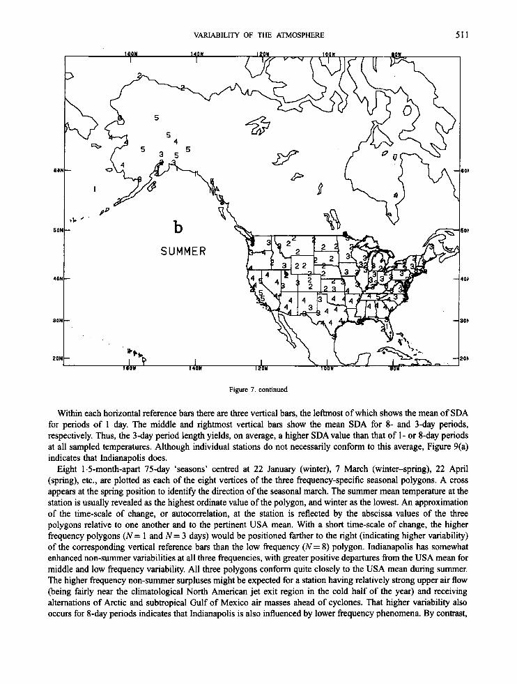
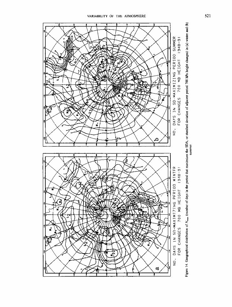
Figure 7. Geographical distribution of N,, (number of days in the period that maximizes the SDA, or standard deviation of adjacent period temperature changes) in (a) winter and (b) summer

to-day) standard deviation for January and July daily mean temperature (same quantity as S DEV, shown in Figure 1 top left inset). Fields of SDA, although not shown here, would reflect the combined effects of the interdiurnal standard deviation and the time-scale of change, which cannot be separated easily without inspecting SDA fields for several period lengths ( N ). One way to characterize both factors is by plotting SDA against the mean temperature itself for a single station, using several values of N in the same plot.

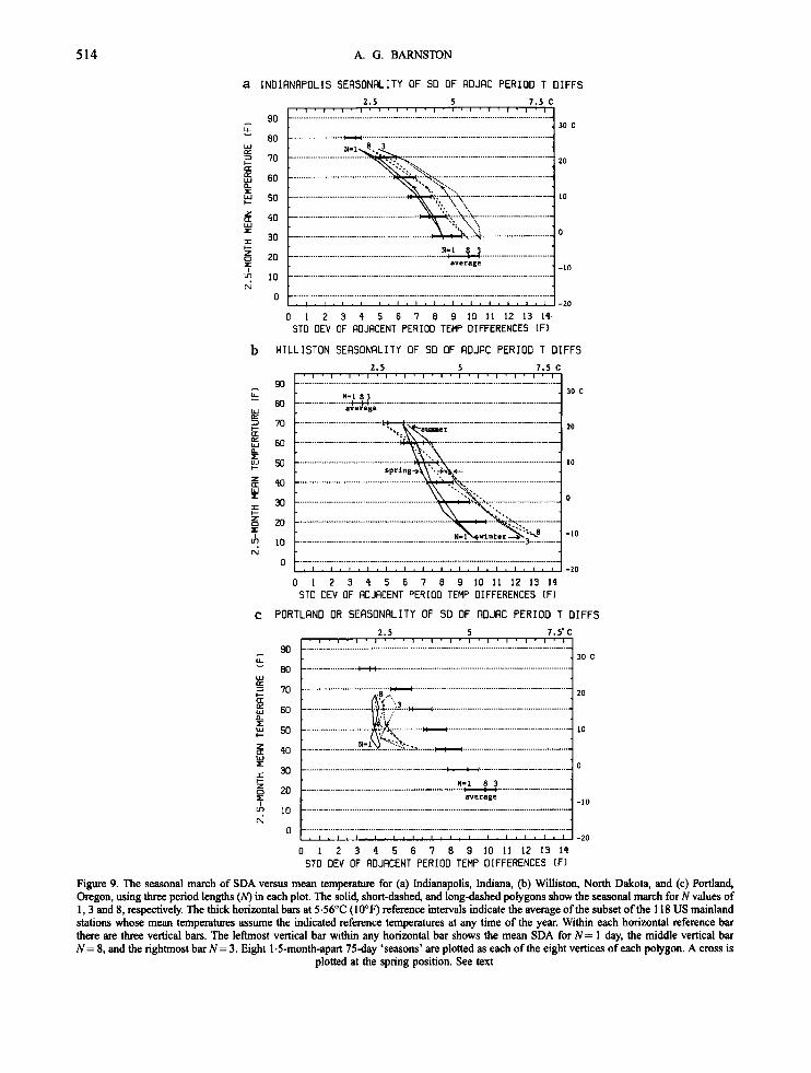
Figure 9(a) is such a plot for Indianapolis. The solid, short-dashed and long-dashed polygons show the seasonal march of SDA versus mean temperature for N values of 1, 3, and 8, respectively. The thick horizontal bars at 5-56°C (10°F) reference intervals indicate the average of the subset of the 1 18 USA mainland stations whose mean temperatures assume the indicated reference temperatures at any time of the year. It is apparent that higher variability at all three time-scales tends to occur with lower mean temperature. This is the case because variations are larger when synoptic disturbances provide opportunities for warm and cold advection. Such disturbances occur most frequently along the latitude of the climatological mean jet, and less frequently far to its north and south. In USA winter, the main and subtropical jets occur over a range of latitudes, allowing much of the country to experience alternations of warm and cold advection. In summer the subtropical jet dissipates and the main jet migrates to the northern border, leaving the low and middle USA latitudes without exposure to major synoptic disturbances. Even the higher mainland US latitudes, which retain some summer warm and cold advection, have weaker temperature variations because the sources of warm and cold advection (Canada/Arctic versus the northern tropics/subtropics) have less contrasting temperatures in summer than in winter.

VARIABILITY OF THE ATMOSPHERE 51 1

Figure 7. continued

Within each horizontal reference bars there are three vertical bars, the leftmost of which shows the mean of SDA for periods of 1 day. The middle and rightmost vertical bars show the mean SDA for 8- and 3-day periods, respectively. Thus, the 3-day period length yields, on average, a higher SDA value than that of 1- or 8-day periods at all sampled temperatures. Although individual stations do not necessarily conform to this average, Figure 9(a) indicates that Indianapolis does.

Eight 1.5-month-apart 75-day ‘seasons’ centred at 22 January (winter), 7 March (winter-spring), 22 April (spring), etc., are plotted as each of the eight vertices of the three frequency-specific seasonal polygons. A cross appears at the spring position to identify the direction of the seasonal march. The summer mean temperature at the station is usually revealed as the highest ordinate value of the polygon, and winter as the lowest. An approximation of the time-scale of change, or autocorrelation, at the station is reflected by the abscissa values of the three polygons relative to one another and to the pertinent USA mean. With a short time-scale of change, the higher frequency polygons (N= 1 and N = 3 days) would be positioned farther to the right (indicating higher variability) of the corresponding vertical reference bars than the low frequency (N= 8) polygon. Indianapolis has somewhat enhanced non-summer variabilities at all three frequencies, with greater positive departures from the USA mean for middle and low frequency variability. All three polygons conform quite closely to the USA mean during summer. The higher frequency non-summer surpluses might be expected for a station having relatively strong upper air flow (being fairly near the climatological North American jet exit region in the cold half of the year) and receiving alternations of Arctic and subtropical Gulf of Mexico air masses ahead of cyclones. That higher variability also occurs for 8-day periods indicates that Indianapolis is also influenced by lower frequency phenomena. By contrast,

512 A. G. BARNSTON

30Y

50N

I

40b

3 0 ~

20b

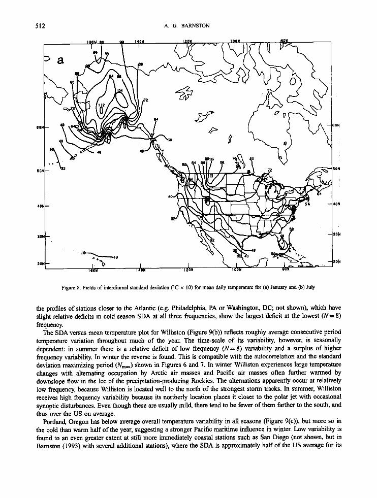
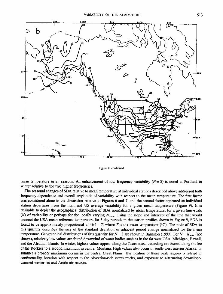
Figure 8. Fields of interdiumal standard deviation (“C x 10) for mean daily temperature for (a) January and (b) July

the profiles of stations closer to the Atlantic (e.g. Philadelphia, PA or Washington, DC; not shown), which have slight relative deficits in cold season SDA at all three frequencies, show the largest deficit at the lowest (N= 8) fiequenc y.

The SDA versus mean temperature plot for Williston (Figure 9(b)) reflects roughly average consecutive period temperature variation throughout much of the year. The time-scale of its variability, however, is seasonally dependent: in summer there is a relative deficit of low frequency ( N = 8 ) variability and a surplus of higher frequency variability. In winter the reverse is found. This is compatible with the autocomlation and the standard deviation maximizing period (N-) shown in Figures 6 and 7. In winter Williston experiences large temperature changes with alternating occupation by Arctic air masses and Pacific air masses often further warmed by downslope flow in the lee of the precipitation-producing Rockies. The alternations apparently occur at relatively low frequency, because Williston is located well to the north of the strongest storm tracks. In summer, Williston receives high frequency variability because its northerly location places it closer to the polar jet with occasional synoptic disturbances. Even though these are usually mild, there tend to be fewer of them farther to the south, and thus over the US on average.

Portland, Oregon has below average overall temperature variability in all seasons Figure 9(c)), but more so in the cold than warm half of the year, suggesting a stronger Pacific maritime influence in winter. Low variability is found to an even greater extent at still more immediately coastal stations such as San Diego (not shown, but in Barnston (1 993) with several additional stations), where the SDA is approximately half of the US average for its


Figure 8. continued

mean temperature in all seasons. An enhancement of low frequency variability ( N = 8 ) is noted at Portland in winter relative to the two higher frequencies.

The seasonal changes of SDA relative to mean temperature at individual stations described above addressed both frequency dependence and overall amplitude of variability with respect to the mean temperature. The first factor was considered alone in the discussion relative to Figures 6 and 7, and the second factor appeared as individual station departures from the mainland US average variability for a given mean temperature (Figure 9). It is desirable to depict the geographical distribution of SDA normalized by mean temperature, for a given time-scale (N) of variability or perhaps for the locally varying N-. Using the slope and intercept of the line that would connect the USA mean reference temperature for 3-day periods in the station profiles shown in Figure 9, SDA is found to be approximately proportional to 46.1 - T, where T is the mean temperature (“C). The ratio of SDA to this quantity describes the size of the standard deviation of adjacent period change normalized for the mean temperature. Geographical distributions of this quantity for N = 3 are shown in Barnston (1 993). For N = N,, (not shown), relatively low values are found downwind of water bodies such as in the far west USA, Michigan, Hawaii, and the Aleutian Islands. In winter, highest values appear along the Texas coast, extending northward along the lee of the Rockies to a second maximum in central Montana. High values also occur in south-west interior Alaska. In summer a broader maximum occurs in the central Great Plains. The location of these peak regions is related to continentality, location with respect to the advection-rich storm tracks, and exposure to alternating downslope- warmed westerlies and Arctic air masses.

514 A. G. BARNSTON

a INOIRNRPOLIS SEASONALITY OF so OF AOJRC PERIOD T DIFFS 2.5 5 7.5 c

1 . I ' I ' I ' I ' I ' I ' I ' I ' I ' I ' I ' 1 ' 1 go 30 C -

............

60 ...........................

10

0

_ _ ............ ..... ...... ....._

, . , . , . , . , . I . I . I . I . I . l . 1 . l . 1 -20

0 1 2 3 4 5 6 7 8 9 1 0 1 1 1 2 1 3 1 4 ~ STD DEV OF ADJACENT PERIOD TEMP DIFFERENCES [FI

b WILLISTON SEASONRLITY OF SO OF ADJRC PERIOD T DIFFS

N-1 8 3 w)

average

I lo k;, ** ...................

'+\;- .................. 1 0

.. .... " ..-.:.

.. "interx=\* * -10

0 I . I . I . I . I , I . I . I . I , I . I . I I I . I -20

0 1 2 3 4 5 6 7 B 9 1 0 1 1 1 2 1 3 1 4 STD DEV OF RDJACENT PERIOO TEMP DIFFERENCES IF1

c PORTLAND OR SEASONRLITY OF SO OF FlDJRC PERIOD T D I F F S

90

80

70

60

50

- 1L # U

Q x

s 40

r 30 5 20

W r

k-

JL

L+ 10 N

n

........ ............... " To w)

......................................... 20

- ............................. ...- .

............................... ........... - .................. " ........................... 10 1 .:>a ........ - -

................................................................... . .............. lo -..... N-1 8 3 ..................................................................... )

average ...................................................................

0 1 2 3 4 5 6 7 8 9 1 0 1 1 1 2 1 3 1 4 STO DEV OF ADJACENT PERIOD TEMP OIFFERENCES ( F l

Figure 9. The seasonal march of SDA versus mean temperature for (a) Indianapolis, Indiana, (b) Williston, North Dakota, and (c) Portland, Oregon, using three period lengths (N) in each plot. The solid, short-dashed, and long-dashed polygons show the seasonal march for N values of 1,3 and 8, respectively. The thick horizontal bars at 5.56"C (10'F) reference intervals indicate the average of the subset of the 118 US mainland stations whose mean temperatures assume the indicated reference temperatures at any time of the year. Within each horizontal reference bar there are three vertical bars. The leftmost vertical bar within any horizontal bar shows the mean SDA for N = 1 day, the middle vertical bar N = 8, and the rightmost bar N = 3. Eight 1.5-month-apart 75-day 'seasons' are plotted as each of the eight vertices of each polygon. A cross is

plotted at the spring position. See text


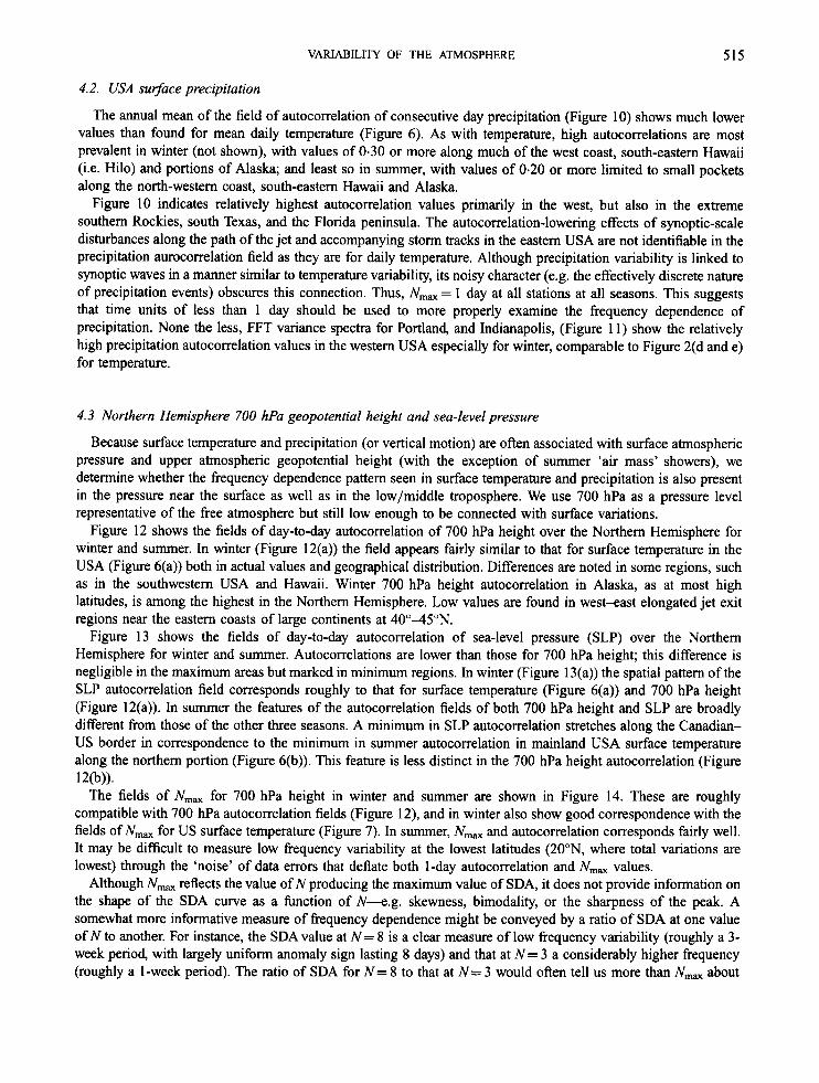
4.2. USA surface precipitation

The annual mean of the field of autocorrelation of consecutive day precipitation (Figure 10) shows much lower values than found for mean daily temperature (Figure 6). As with temperature, high autocorrelations are most prevalent in winter (not shown), with values of 0.30 or more along much of the west coast, south-eastern Hawaii (i.e. Hilo) and portions of Alaska; and least so in summer, with values of 0.20 or more limited to small pockets along the north-western coast, south-eastern Hawaii and Alaska.

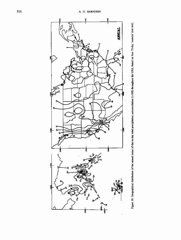
Figure 10 indicates relatively highest autocorrelation values primarily in the west, but also in the extreme southern Rockies, south Texas, and the Florida peninsula. The autocorrelation-lowering effects of synoptic-scale disturbances along the path of the jet and accompanying storm tracks in the eastern USA are not identifiable in the precipitation aurocorrelation field as they are for daily temperature. Although precipitation variability is linked to synoptic waves in a manner similar to temperature variability, its noisy character (e.g. the effectively discrete nature of precipitation events) obscures this connection. Thus, N,, = 1 day at all stations at all seasons. This suggests that time units of less than 1 day should be used to more properly examine the frequency dependence of precipitation. None the less, FFT variance spectra for Portland, and Indianapolis, (Figure 11) show the relatively high precipitation autocorrelation values in the western USA especially for winter, comparable to Figure 2(d and e) for temperature.

4.3 Northern Hemisphere 700 hPa geopotential height and sea-level pressure

Because surface temperature and precipitation (or vertical motion) are often associated with surface atmospheric pressure and upper atmospheric geopotential height (with the exception of summer 'air mass' showers), we determine whether the frequency dependence pattern seen in surface temperature and precipitation is also present in the pressure near the surface as well as in the low/middle troposphere. We use 700 hPa as a pressure level representative of the free atmosphere but still low enough to be connected with surface variations.

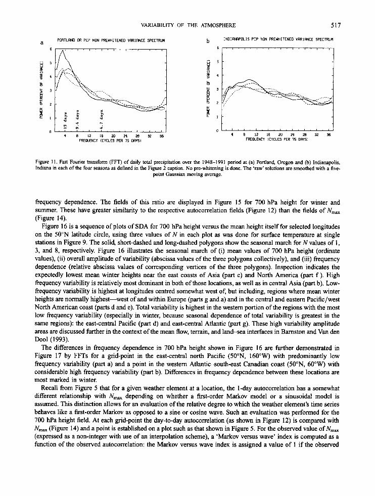
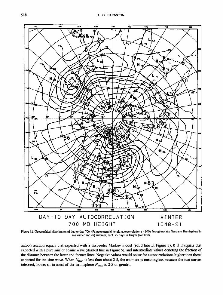
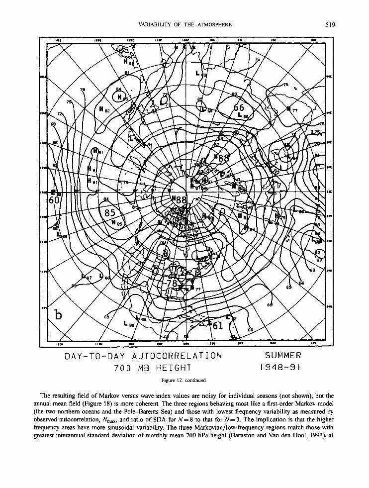
Figure 12 shows the fields of day-to-day autocorrelation of 700 hPa height over the Northern Hemisphere for winter and summer. In winter (Figure 12(a)) the field appears fairly similar to that for surface temperature in the USA (Figure 6(a)) both in actual values and geographical distribution. Differences are noted in some regions, such as in the southwestern USA and Hawaii. Winter 700 hPa height autocorrelation in Alaska, as at most high latitudes, is among the highest in the Northern Hemisphere. Low values are found in west-east elongated jet exit regions near the eastern coasts of large continents at 40"-45"N.

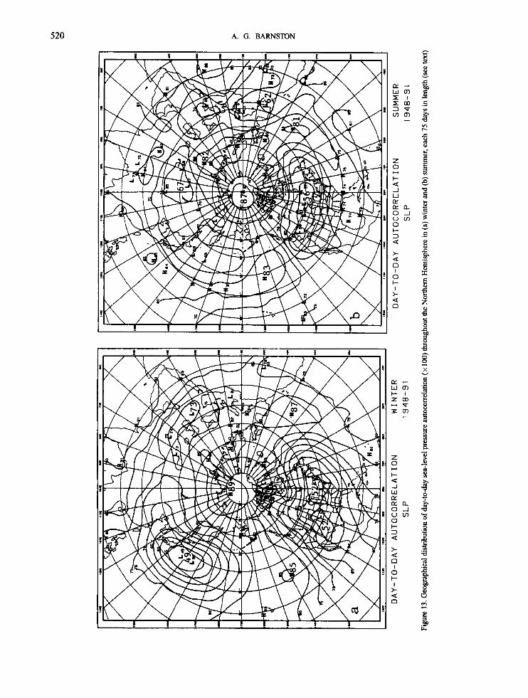
Figure 13 shows the fields of day-to-day autocorrelation of sea-level pressure (SLP) over the Northern Hemisphere for winter and summer. Autocorrelations are lower than those for 700 hPa height; this difference is negligible in the maximum areas but marked in minimum regions. In winter (Figure 13(a)) the spatial pattern of the SLP autocorrelation field corresponds roughly to that for surface temperature (Figure 6(a)) and 700 hPa height (Figure 12(a)). In summer the features of the autocorrelation fields of both 700 Wa height and SLP are broadly different from those of the other three seasons. A minimum in SLP autocorrelation stretches along the Canadian- US border in correspondence to the minimum in summer autocorrelation in mainland USA surface temperature along the northern portion (Figure 6(b)). This feature is less distinct in the 700 hPa height autocorrelation (Figure

The fields of N,,, for 700 hPa height in winter and summer are shown in Figure 14. These are roughly compatible with 700 hPa autocorrelation fields (Figure 12), and in winter also show good correspondence with the fields of N,, for US surface temperature (Figure 7). In summer, NmaX and autocorrelation corresponds fairly well. It may be difficult to measure low frequency variability at the lowest latitudes (20"N, where total variations are lowest) through the 'noise' of data errors that deflate both 1-day autocorrelation and Nmax values.

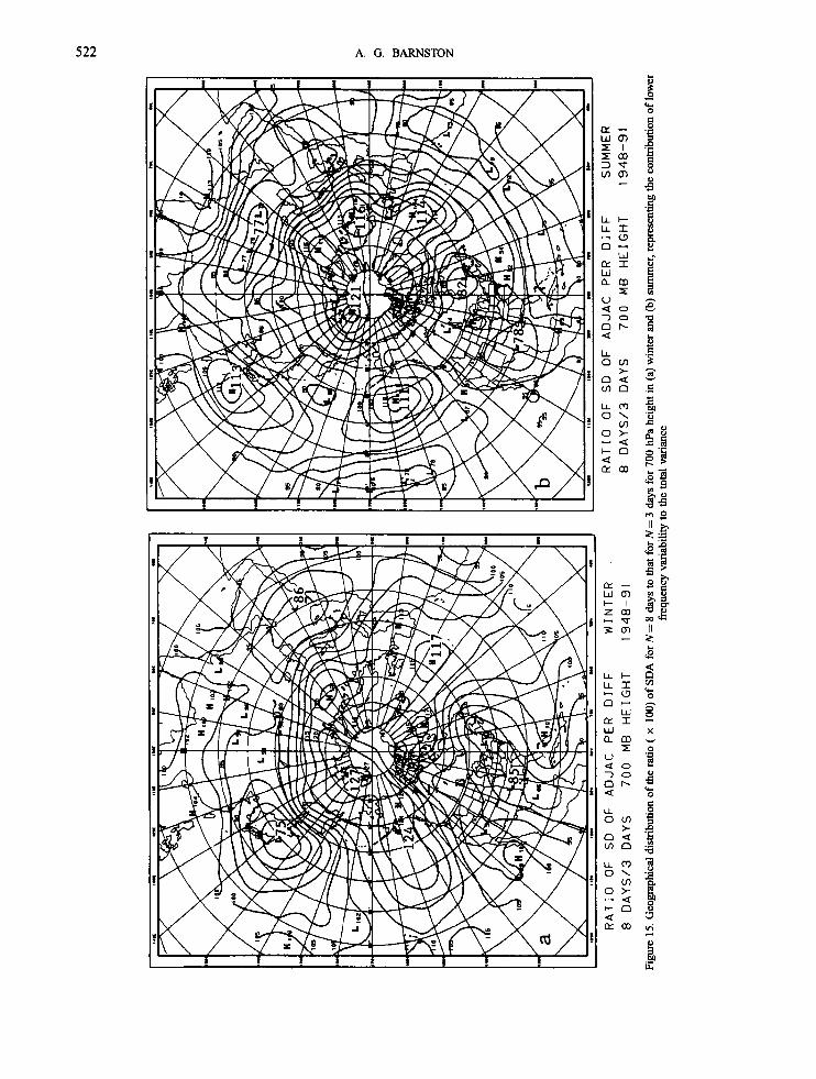
Although N,, reflects the value of N producing the maximum value of SDA, it does not provide information on the shape of the SDA curve as a function of N--e.g. skewness, bimodality, or the sharpness of the peak. A somewhat more informative measure of frequency dependence might be conveyed by a ratio of SDA at one value of N to another. For instance, the SDA value at N = 8 is a clear measure of low frequency variability (roughly a 3- week period, with largely uniform anomaly sign lasting 8 days) and that at N = 3 a considerably higher frequency (roughly a 1-week period). The ratio of SDA for N = 8 to that at N = 3 would often tell us more than N,, about

12(b)).

Figu

re 1

0. G

eogr

aphi

cal d

istrib

utio

n of

the annual m

ean

of d

ay-to

day total

prec

ipita

tion a

utoc

orre

latio

n (x

100)

thro

ugho

ut th

e U

SA

, bas

ed o

n four 7

5-da

y ‘seasons’ (s

ee t

ext)

?

F


b INOIRNAPOLIS PCP NON PREWHITENED VRRIRNCE SPECTRUM PORTLAND OR PCP NDN PREWHITENED VRRIRNCE SPECTRUM

t a 12 16 m 24 za 32 36 FREQUENCY (CYCLES PER 75 DRYS1

4 8 12 16 20 24 za u 36 FREOUENCY [CYCLES PER 75 DRYS1

Figure 1 1 . Fast Fourier transform (FFT) of daily total precipitation over the 1948-1991 period at (a) Portland, Oregon and (b) Indianapolis, Indiana in each of the four seasons as defined in the Figure 2 caption. No pre-whitening is done. The 'raw'solutions are smoothed with a five-

point Gaussian moving average.

frequency dependence. The fields of this ratio are displayed in Figure 15 for 700 hPa height for winter and summer. These have greater similarity to the respective autocorrelation fields (Figure 12) than the fields of N,, (Figure 14).

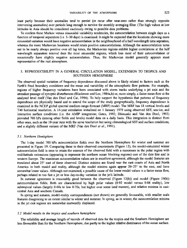
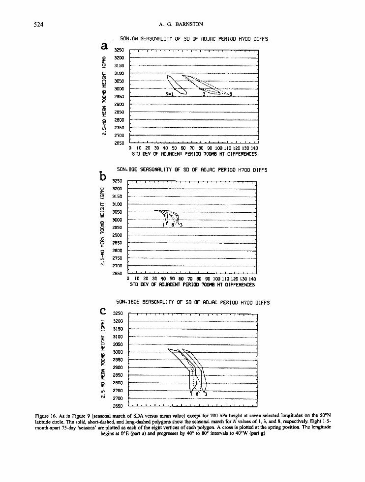
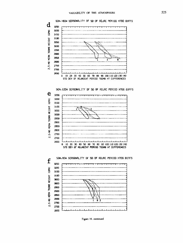
Figure 16 is a sequence of plots of SDA for 700 hPa height versus the mean height itself for selected longitudes on the 50'" latitude circle, using three values of N in each plot as was done for surface temperature at single stations in Figure 9. The solid, short-dashed and long-dashed polygons show the seasonal march for N values of 1, 3, and 8, respectively. Figure 16 illustrates the seasonal march of (i) mean values of 700 hPa height (ordinate values), (ii) overall amplitude of variability (abscissa values of the three polygons collectively), and (iii) frequency dependence (relative abscissa values of corresponding vertices of the three polygons). Inspection indicates the expectedly lowest mean winter heights near the east coasts of Asia (part c) and North America (part f ). High frequency variability is relatively most dominant in both of those locations, as well as in central Asia (part b). Low- frequency variability is highest at longitudes centred somewhat west of, but including, regions where mean winter heights are normally highest-west of and within Europe (parts g and a) and in the central and eastern Pacific/west North American coast (parts d and e). Total variability is highest in the western portion of the regions with the most low frequency variability (especially in winter, because seasonal dependence of total variability is greatest in the same regions): the east-central Pacific (part d) and east-central Atlantic (part g). These high variability amplitude areas are discussed further in the context of the mean flow, terrain, and land-sea interfaces in Barnston and Van den Do01 (1993).

The differences in frequency dependence in 700 hPa height shown in Figure 16 are further demonstrated in Figure 17 by FFTs for a grid-point in the east-central north Pacific (50"N, 16O"W) with predominantly low frequency variability (part a) and a point in the western Atlantic-south-east Canadian coast (50"N, 60"W) with considerable high frequency variability (part b). Differences in frequency dependence between these locations are most marked in winter.

Recall from Figure 5 that for a given weather element at a location, the 1-day autocorrelation has a somewhat different relationship with N,, depending on whether a first-order Markov model or a sinusoidal model is assumed. This distinction allows for an evaluation of the relative degree to which the weather element's time series behaves like a first-order Markov as opposed to a sine or cosine wave. Such an evaluation was performed for the 700 hPa height field. At each grid-point the day-to-day autocorrelation (as shown in Figure 12) is compared with N,, (Figure 14) and a point is established on a plot such as that shown in Figure 5 . For the observed value of N,, (expressed as a non-integer with use of an interpolation scheme), a 'Markov versus wave' index is computed as a fhction of the observed autocorrelation: the Markov versus wave index is assigned a value of 1 if the observed

518 A. G. BARNSTON

7 0 0 MB H E I G H T 1948-9 1 Figure 12. Geographical distribution of day-to-day 700 hPa geopotential height autocorrelation ( x 100) throughout the Northern Hemisphere in

(a) winter and (b) summer, each 75 days in length (see text)

autocorrelation equals that expected with a first-order Markov model (solid line in Figure 5) , 0 if it equals that expected with a pure sine or cosine wave (dashed line in Figure 5) , and intermediate values denoting the fraction of the distance between the latter and former lines. Negative values would occur for autocorrelations higher than those expected for the sine wave. When N,, is less than about 2.5, the estimate is meaningless because the two curves intersect; however, in most of the hemisphere N,, is 2.5 or greater.


DAY-TO-DAY A U T O C O R R E L A T I O N SUMMER 7 0 0 MB HEIGHT 1948-9 1

Figure 12. continued

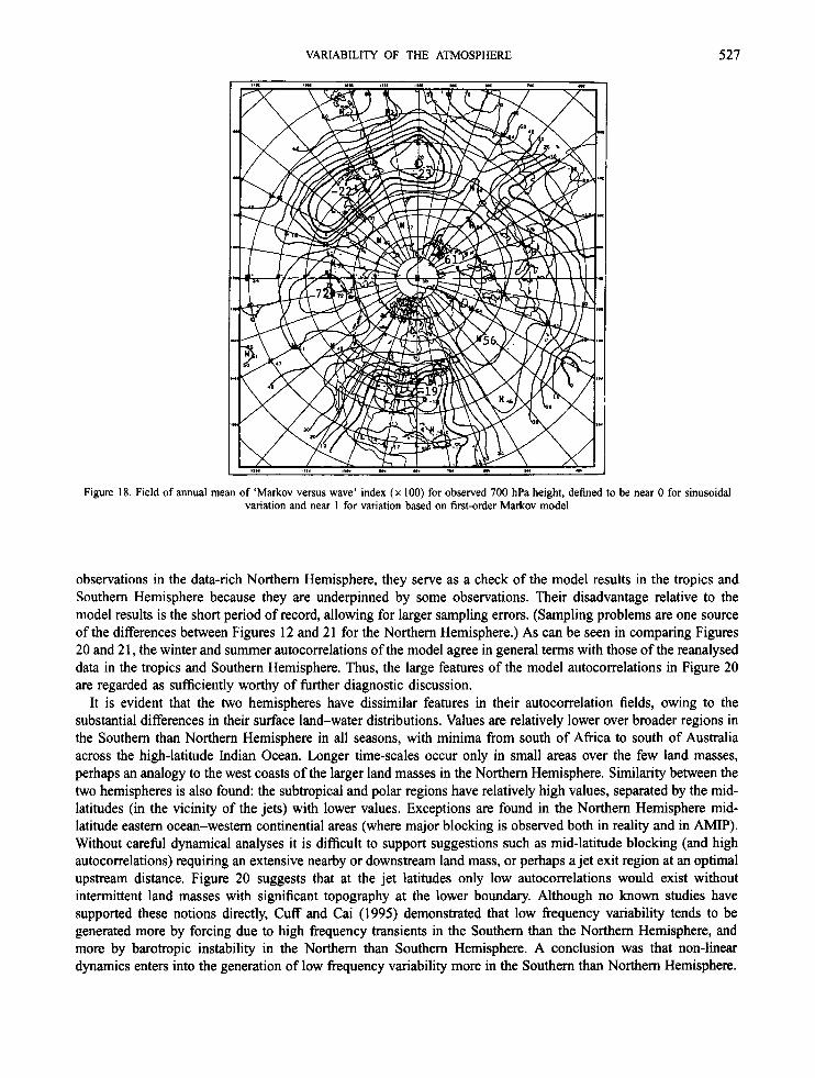
The resulting field of Markov versus wave index values are noisy for individual seasons (not shown), but the annual mean field (Figure 18) is more coherent. The three regions behaving most like a first-order Markov model (the two northern oceans and the Pole-Barents Sea) and those with lowest frequency variability as measured by observed autocorrelation, N-, and ratio of SDA for N = 8 to that for N = 3. The implication is that the higher frequency areas have more sinusoidal variability. The three Markovian/low-frequency regions match those with greatest in temual standard deviation of monthly mean 700 hPa height (Bamston and Van den Dool, 1993), at

520 A. G . BARNSTON

[ L - w o I I SOD 3 v v)o c

Z 0

t- U _I w & L Y L 0 1 urn 0 c 3

w

a

a >-

0 I 0 t- I t U 0

[ L - w c n t - I ZOD - v x o -

Z 0

t- U J W LY LTa 0 1 vv) 0 I- 3 U

t U 0

I 0 I- I t

0

-

a

16

-8b

61

lH

31

3H

8W

OOL S

33

NV

H3

8

03

813W

WflS

aO

Iti13d

3N

IZIW

IXV

W-O

S

NI

SA

Va

'O

N

16

-8b

61

lH

31

3H

8W

OOL

S3

3N

VH

3

80

3

83

1N

IM 0

0I8

3d

3N

IZIW

IXV

W-O

S

NI S

AV

O 'ON

*n.

I I”

11”

I

I.

a.

u

RA

TIO

OF

SD

O

F A

DJA

C

PE

R D

IFF

W

INT

ER

8

DA

YS

/3

DA

YS

7

00

ME

H

EIG

HT

1

94

8-9

1

RA

TIO

OF

SD

O

F A

DJA

C

PE

R D

IFF

S

UM

ME

R

8

DA

YS

/3

DA

YS

7

00

M

I3

HE

IGH

T

19

48

-91

Figu

re 1

5. G

eogr

aphi

cal d

istrib

utio

n of

the

ratio

( x

100)

of S

DA

for N

= 8

days

to th

at f

or N= 3

days

for

700

hPa

heig

ht in

(a)

win

ter

and

@)

sum

mer

, representing

the

cont

ribut

ion

of lo

wer

h

qu

ency

var

iabi

lity

to th

e to

tal v

aria

nce


least partly because their anomalies tend to persist (or recur after near-zero rather than strongly opposite intervening anomalies) over periods long enough to survive the monthly averaging filter. (The high values at low latitudes in Asia should be considered cautiously owing to possible data problems.

To confirm these Markov versus sinusoidal variability tendencies, the autocorrelation between single days as a function of temporal separation (i.e. 3-30 days) is examined. It might be expected that the locations showing more sinusoidal variation would have negative autocorrelation in the neighbourhood of a half-wavelength time sepration, whereas the more Markovian locations would retain positive autocorrelations. Although the autocorrelation turns out to be nearly always positive over all lag times, the Markovian regions exhibit higher correlations at the half wavelength separation interval than the most sinusoidal regions, which lose most of their autocorrelation or occasionally have slightly negative autocorrelation. Thus, the Markovian model generally appears most representative of the real atmosphere.

5 . REPRODUCIBILITY IN A GENERAL CIRCULATION MODEL; EXTENSION TO TROPICS AND SOUTHERN HEMISPHERE

The observed spatial variation of frequency dependence discussed above is likely related to factors such as the Earth's fixed boundary conditions and the mean and variability of the atmospheric flow patterns. For example, regions of higher frequency variations have been associated with storm tracks underlying a jet axis and the attendant passage of synoptic disturbances (Blackmon and Lee, 1984a,b) or, more simply, a faster mean flow at the analysed level itself (Van den Do01 and Cai, 1994). To help support the hypothesis that patterns of frequency dependence are physically based and to estend the scope of the study geographically, frequency dependence is examined in the NCEP global spectral medium-range-forecast (MRF) model. The MRF has 18 vertical levels and T40 horizontal resolution. A 1Cyear simulation initialized on 1 January 1979 using observed SST, sea-ice, and interactive surface conditions (i.e. the AMIP integration; Gates, 1992; Ebisuzaki and Van den Dool, 1993) provided 700 hPa (among other fields and levels) model data on a daily basis. This integration is distinct from other ones, such as the 10-year runs with the same resolution but using climatological SST and surface conditions, and a slightly different version of the MRF (Van den Do01 et al., 1991).

5.1. Northern Hemisphere

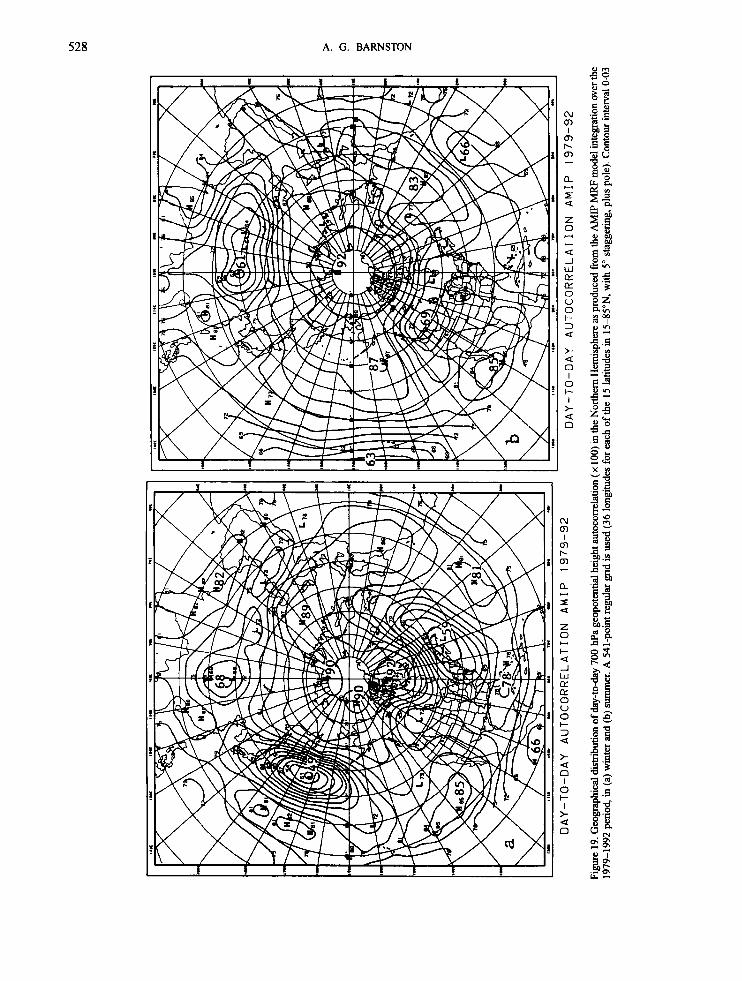
The 1-day model 700 hPa autocorrelation fields over the Northern Hemisphere for winter and summer are presented in Figure 19. Comparing these to their observed counterparts (Figure 12), the model-simulated winter autocorrelation field is seen to retain the essence of the observed field with a maximum in the polar region with mid-latitude extensions (appearing to represent the northern ocean blocking regions) east of the date line and in western Europe. The maximum autocorrelation values are in excellent agreement, although the model features are translated about 25" east of these observed. Distinct minima are found near the east coasts of Asia and North America in both model and reality, although the model minima again appear 20-25" to the east, and have somewhat lower values. Although not examined, a possible cause of the lower model values is a faster mean flow, perhaps related to too fast a jet or less day-to-day variation in the jet's latitude.

In summer agreement is reasonably good between the observed (Figure 120)) and model (Figure 19(b)) autorcorrelation fields. Both are characterized by high polar values (0.92 model versus 0.88 reality), low subtropical values (largely 0.60s to low 0.70s, but higher over some land masses), and relative minima in east- central Asia and southern Canada.

In spring and autumn, model-reality correspondences (not shown) are generally favourable, with smaller scale features disagreeing to an extent similar to winter and summer. In spring, as in winter, the autocorrelation minima in the jet exit regions are somewhat eastwardly displaced.

5.2 Model results in the tropics and southern hemisphere

The reliability and average length of records of observed data for the tropics and the Southern Hemisphere are less favourable than for the Northern Hemisphere, due partly to the higher relative dominance of the ocean surface.

524 A. G . BARNSTON

. 50N.OW SERSONRLITY OF SO OF RDJRC PERIOD H700 OIFFS

3250

3200

3150

3100

3050 3000

2950

2900

2850

2800

2750

2700

2650

1 ' I ' I ' I ' I ~ I . I ' I . I ~ I ' I ' I . I ' l

...................................... "...".. " ....-

...-......... ~ I..__ " .........--

............................. -..- ................... .... " ....... ".._ "_..".._ ......

0 10 20 30 40 50 60 70 80 90 100 110 120 130 140 STO E V OF RDJRCENT PERIOD 700).(8 HT DIFFERENCES

50N.80E SEASONALITY OF SO OF ROJRC PERIOD H700 DIFFS

3250

3200

3150

3100

3050

3000 2950

2900

2850

2800

2750

2700

2650

1 ' 1 ' I ~ I ' I ~ I ~ I ~ I . I ' I ' I ~ I ~ I ' I

"..-...............I.-- ................................ I - ............ .................................................. ~ ........

.............................................. ~ ...... ~ ~

......................... 1 ........

..................... ~ ~ "

.............. ~ .... "..

........................... - .

0 10 20 30 40 50 60 70 80 90 100 110 120 130 140 STD DEV OF #lJACEHT PERIW 7 0 m HT DIFFERENCES

50N.16DE SEASONALITY OF SO OF AOJRC PERIOD H700 OIFFS

3250

3200

3150

3100

3050

3000 2950

2900

2850

2800

2750

2700

2650

................ ........................ .........

. .. .................... ._..__."_."I ....... ..-.. ----.... .I

I . 1 . 1 . I . I . I . I . I . I . I . 1 . 1 . I . I

Figure 16. As in Figure 9 (seasonal march of SDA versus mean value) except for 700 hPa height at seven selected longitudes on the 50"N latitude circle. The solid, short-dashed, and long-dashed polygons show the seasonal march for N values of 1, 3, and 8, respectively. Eight 1.5- month-apart 7Sday 'seasons' are plotted as each of the eight vertices of each polygon. A cross is plotted at the spring position. The longitude

begins at O"E (part a) and progresses by 40" to 80" intervals to 40"W (part g)


e

P P 0

3 Y f 0

In N

f

50N.160W SEASONALITY OF SO OF AOJAC PERIOO H700 DIFFS

3250 . I . I . , , , . I . I ' I . I ' I . I . I . I . I , I

3200 - .................................................................................. ~ ..I.I_

3 150

3100

I ............................................................... "

- .............. ~ .... ~ ...........................................................................................................

2700 2650

_ " " "

~ ' " ~ ' ~ ' ~ ' ~ ' ~ ' ~ ' 1 ' ~ ' ~ ' " ~ ' ' 1

0 10 20 30 40 50 60 70 80 90 100 110 120 130 140 STD DEV OF RDJRCENT PERIOD 7DOME HT DIFFERENCES

SON.120W SEASONALITY OF SO OF ADJRC PERIOD H700 DIFFS

3250

3200

3150

3100

3050

3000 2950

2900 2850

2800

2750

2700 2650

I ................................... "

....................... .................................................................... -

............ ..................................................... I- ....... " .... " .......... _- ...... ...................................................... - I.."".." .... I.." .-..-.. ~ ..... ~ .... ~ ~ ....-.............- ...... " ...................................................................................... "

0 10 20 30 40 50 60 70 80 90 100 110 120 130 140 STD DEV OF WJRCENT PERIOO 7M)MB HT DIFFERENCES

50Nt80W SERSONALITY OF SO OF ADJAC PERIOO H700 DIFFS

3250 I - I - / - I . I . I 9 1 . i , I - 1 * 1 . 1 . I

3200 _ " ... "...................- _.."_ 3 150

3100

3050 3M)o 2950

-... "......._.."I" .. I-....-.-- I .....-...- " .-..-... I - _." ........ " ~ " ._

............ _.I "." I--.... ".._I

....... ...-....... "--.--..-..........I-._..- ---- ~ .......--_ ... ~

-.- -.-.- " .-..-..- 2850

2800

I .--. I .

- ......... ~ ............... " - ............. - ..-.....-........... "._ 1 0 3

2750

2700

_..._..._ ~ .- ................................................................... - _ ~ ._._ .............................................. ~ ..._.........__

2650 ' l . l . l . l . l " . l . ' . ' . l I 1 . l . l . l


526

I ~ , ~ , ~ I . , . , . , . , . , . , . , . , . ~ ' ~

-........ .......... ""..I ............... ~ ..... " ........... ............. ............................. ~ ..... " ~

- ............

A. G. BARNSTON

50N.40W SEASONALITY OF SO OF RDJAC PERIOO H700 DIFFS

3250

3200

3150

3100

3050

3000

2950 2900

2850

2800

2750

2700

2650

t i ........... . .- ..... ".I --.- ""_. -I t 4

....-.-.. ...... 1 . 1 . 1 . 1 . 1 . 1 . 1 . 1 . 1 . 1 . 1 . 1 . 1 .

o 10 20 30 40 50 60 70 ao 90 100 110 120 130 140 STD DEV OF RDJRCENT PERIOD 7 0 M HT DIFFERENCES

700ME HT 150N.160Wl PREWHITENED VRRIRNCE SPECTRUN

4 8 12 16 20 24 28 32 98 FREQUENCY [CYCLES PER 75 ORYSl


700HB HT [50N.60W1 PREWHITENED VRRIRNCE SPECTRUM

E t t 1

Figure 17. (a) Fast Fourier transform (FFT) of daily 700 hPa height over the 1948-1991 period at SOON, 160"W during 75-day periods representing each of the four 'seasons'. The solid curve denotes winter (16 December to 29 February), the small dashed curve spring, medium dashed curve summer, and large dashed curve autumn. The spectrum is pre-whitened by using the change between the previous day's temperature multiplied by 0.707 and the present day's temperature. The noisy 'raw' solutions have been smoothed with a five-point Gaussian

moving average. @) As in (a) except for 50"N, 60"W

Because the gross features of the observed 1-day autocorrelation fields at 700 hPa are well reproduced in the Northern Hemisphere by the 14-year AMP model run (see previous subsection), we examine the remaining areas of the globe using the model data. Although a quantitative comparison between model and observed data is prohibited in the tropics and Southern Hemisphere by the sparseness of observed data, some support for the model- derived autocorrelations is provided by autocorrelations based on independently reanalysed estimates of observed data over the 1985-1994 period. The reanalysed fields are derived using the dynamical NCEP MRF model using 28 levels and T62 horizontal resolution (i.e. greater resolution than the AMIP model), assimilating the available observations (Kalnay et al., 1995).

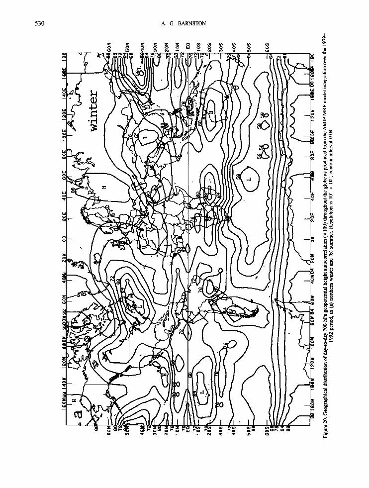
The 1 -day model 700 hPa height autocorrelation fields over the globe (except for 80-90" latitude) for northern winter and summer are presented in Figure 20, which overlaps with Figure 19 but uses a coarser grid. Supporting evidence from reanalysed data for 1985-1994 is shown by their autocorrelation fields for winter and summer (Figure 21). Although the latter cannot provide much improvement over the results shown in Figure 12 for

527 VARIABILITY OF THE ATMOSPHERE

Figure 18. Field of annual mean of ‘Markov versus wave’ index ( x 100) for observed 700 hPa height, defined to be near 0 for sinusoidal variation and near 1 for variation based on first-order Markov model

observations in the data-rich Northern Hemisphere, they serve as a check of the model results in the tropics and Southern Hemisphere because they are underpinned by some observations. Their disadvantage relative to the model results is the short period of record, allowing for larger sampling errors. (Sampling problems are one source of the differences between Figures 12 and 21 for the Northern Hemisphere.) As can be seen in comparing Figures 20 and 2 1 , the winter and summer autocorrelations of the model agree in general terms with those of the reanalysed data in the tropics and Southern Hemisphere. Thus, the large features of the model autocorrelations in Figure 20 are regarded as sufficiently worthy of further diagnostic discussion.

It is evident that the two hemispheres have dissimilar features in their autocomelation fields, owing to the substantial differences in their surface land-water distributions. Values are relatively lower over broader regions in the Southern than Northern Hemisphere in all seasons, with minima from south of Africa to south of Australia across the high-latitude Indian Ocean. Longer time-scales occur only in small areas over the few land masses, perhaps an analogy to the west coasts of the larger land masses in the Northern Hemisphere. Similarity between the two hemispheres is also found: the subtropical and polar regions have relatively high values, separated by the mid- latitudes (in the vicinity of the jets) with lower values. Exceptions are found in the Northern Hemisphere mid- latitude eastern ocean-western continential areas (where major blocking is observed both in reality and in AMIP). Without careful dynamical analyses it is difficult to support suggestions such as mid-latitude blocking (and high autocorrelations) requiring an extensive nearby or downstream land mass, or perhaps a jet exit region at an optimal upstream distance. Figure 20 suggests that at the jet latitudes only low autocorrelations would exist without intermittent land masses with significant topography at the lower boundary. Although no known studies have supported these notions directly, Cuff and Cai (1995) demonstrated that low frequency variability tends to be generated more by forcing due to high frequency transients in the Southern than the Northern Hemisphere, and more by barotropic instability in the Northern than Southern Hemisphere. A conclusion was that non-linear dynamics enters into the generation of low frequency variability more in the Southern than Northern Hemisphere.

DAY-

TO-D

AY AU

TOCO

RREL

ATIO

N AM

IP 19

79-9

2 DA

Y-TO

-DAY

AU

TOCO

RREL

ATIO

N AM

IP 1979-92

Figu

re 1

9. G

eogr

aphi

cal d

istrib

utio

n of

day

-toda

y 70

0 W

a ge

opot

entia

l hei

ght a

utoc

orre

latio

n (x

100)

in th

e N

orth

ern

Hem

isphe

re as

pro

duce

d from th

e M

E' M

RF

mod

el in

tegr

atio

n ov

er th

e 19

79-1

992

perio

d, in

(a) w

inte

r an

d @

) su

mmer

. A 5

41-p

oint

regular g

rid is

use

d (3

6 lo

ngitu

des f

or e

ach

of th

e 15

latit

udes

in 1

5-8S

oN, w

ith 5

" st

agge

ring,

plu

s pol

e). C

onto

ur in

terv

al 0

.03


Figure 20 indicates that autocorrelation in the tropics tends to be somewhat lower than in the subtropics of both hemispheres, but much greater than those in the storm track regions of the mid-latitudes. The tropics (and, somewhat, the subtropics) are known to have a strong interannual component of variability, such as that associated with ENSO or longer multi-year regimes, both of which may be potentially predictable. If the interannual variability were excluded from the autocorrelation computations shown in Figure 20, autocorrelation values in the tropics would be lower, reflecting a relative lack of variability on time-scales of 2 days or more within an individual season.

5. SUMMARY AND CONCLUSIONS

In this study, time-scales of variability of several weather elements are explored by season and location in mainly the Northern Hemisphere. The major motivation is increased descriptive understanding of this aspect of the atmosphere, and implications regarding long-range forecasting. Long-range forecasts have greatest potential in seasons/regions having a strong low frequency component of variability. However, this potential has so far been more realizable for low frequency variability related to boundary conditions (e.g. ENSO) than to internal dynamics (e.g. blocking in the northern ocean basins).

New as well as existing measures of persistence and frequency dependence are used and intercompared. The standard deviation of the differences between adjacent period means (SDA), when compared over a range of period lengths, reflects both autocorrelations and (if applicable) cycle time. The SDA-maximizing number of consecutive days in the adjacent periods (NmaX) is a simple but meaningful general measure of frequency dependence in a time series. A more informative parameter is the ratio of SDA for one period length to that for another, which can be regarded as a ratio of outputs of band-pass filters targeting differing frequency bands.

The amplitude (or amount) of variability tends to vary as a function of latitude and the geographical environment (i.e. higher latitude and continentality of upstream environment tend to increase variability). Variability is greatest during the colder seasons at most locations (Figure 9). The geographic distribution of the dominant frequencies of variability for each season are examined for USA surface temperature and precipitation, and for Northern Hemisphere SLP and 700 hPa geopotential height. For the latter field, data from the AMIP integration of the NCEP general circulation model as well as observed data are examined, and, with some displacement and intensity errors, the general features using observed data are well reproduced in the model data. Because the dominant frequencies tend to vary in parallel across all observed fields in the USA (including Alaska and Hawaii), the 700 hPa height frequency dependence results are regarded as an adequate description for any of the variables studied here. The examination is thus extended to the tropics and Southern Hemisphere using model 700 hPa heights. However, caution should be used in generalizing results to the other fields in the tropics, where quasi-geostrophic theory is inapplicable. Unlike in virtually all of the extratropics, interannual autocorrelation is a significant component of total autocorrelation in the tropics.

As found in many other studies, weather variables in general vary at relatively low frequency (long periods) at high latitudes and also, to a lesser extent, at subtropical latitudes. In Northern Hemisphere mid-latitudes low frequency variability occurs to the greatest extent over the eastern and central North Pacific and North Atlantic oceans (where blocking episodes are observed most commonly). High frequency variability occurs over the western oceans and the eastern and central parts of the continents, where jet exit regions and fast-moving synoptic- scale weather disturbances are found most frequently. The longitudinal variation of mid-latitude frequency dependence, although large in the Northern Hemisphere, is substantially less in the Southern Hemisphere. This may be the case because of the comparative absence of large, topographically significant land masses with separation distance conducive to longitudinal variations in jet intensity and attendant storm tracks and their associated higher frequency variability.

The tropics, although not strongly dominated by low frequency intraseasonal variations, have a relatively large contribution from interannual oscillations. Such oscillations represent interseasonal and interannual variation related to ENSO, the tropospheric QBO, and decadal regimes, all of which affect the tropics and subtropics more strongly than the higher latitudes, Accordingly, these regions may be amenable to climate forecast skill at time- scales beyond those considered here.

VI

W 0

? n m

Figu

re 2

0. G

eogr

aphi

cal d

istri

butio

n of d

ay-to

day

700

hPa

geop

oten

tial h

eigh

t aut

ocor

rela

tion (

x 1

00) t

hrou

ghou

t the

glo

be as

pro

duce

d from t

he A

MlP

h4RF

mod

el in

tegr

atio

n ov

er th

e 19

79-

1992

per

iod,

in (

a) n

orth

em w

inte

r an

d (b

) su

mm

er. R

esol

utio

n is

10"

x lo

", co

ntou

r int

erva

l 0.04

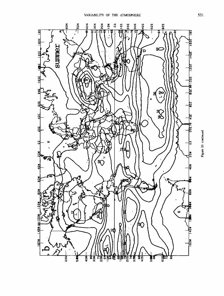
VARIABILITY OF THE ATMOSPHERE 53 1

0 N

b k

532 A. G . BARNSTON

100 1 2ow 0 60E 12OE I80

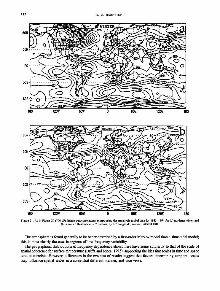
Figure 21. As in Figure 20 (700 hPa height autocorrelation) except using the reanalysis global data for 1985-1994 for (a) northern winter and (b) summer. Resolution is 5" latitude by 10" longitude; contour interval 0.04

The atmosphere is found generally to be better described by a first-order Markov model than a sinusoidal model; this is most clearly the case in regions of low frequency variability.

The geographical distributions of frequency dependence shown here have some similarity to that of the scale of spatial coherence for surface temperature (Briffa and Jones, 1993), supporting the idea that scales in time and space tend to correlate. However, differences in the two sets of results suggest that factors determining temporal scales may influence spatial scales in a somewhat different manner, and vice versa.


ACKNOWLEDGEMENTS

Dr James Purser provided substantial guidance on the mathematical evaluation of the SDA measure as a band-pass filter. Zoltan Toth, Huug Van den Dool, and Edward O’Lenic offered helpfil suggestions for an earlier version of this manuscript.

APPENDIX

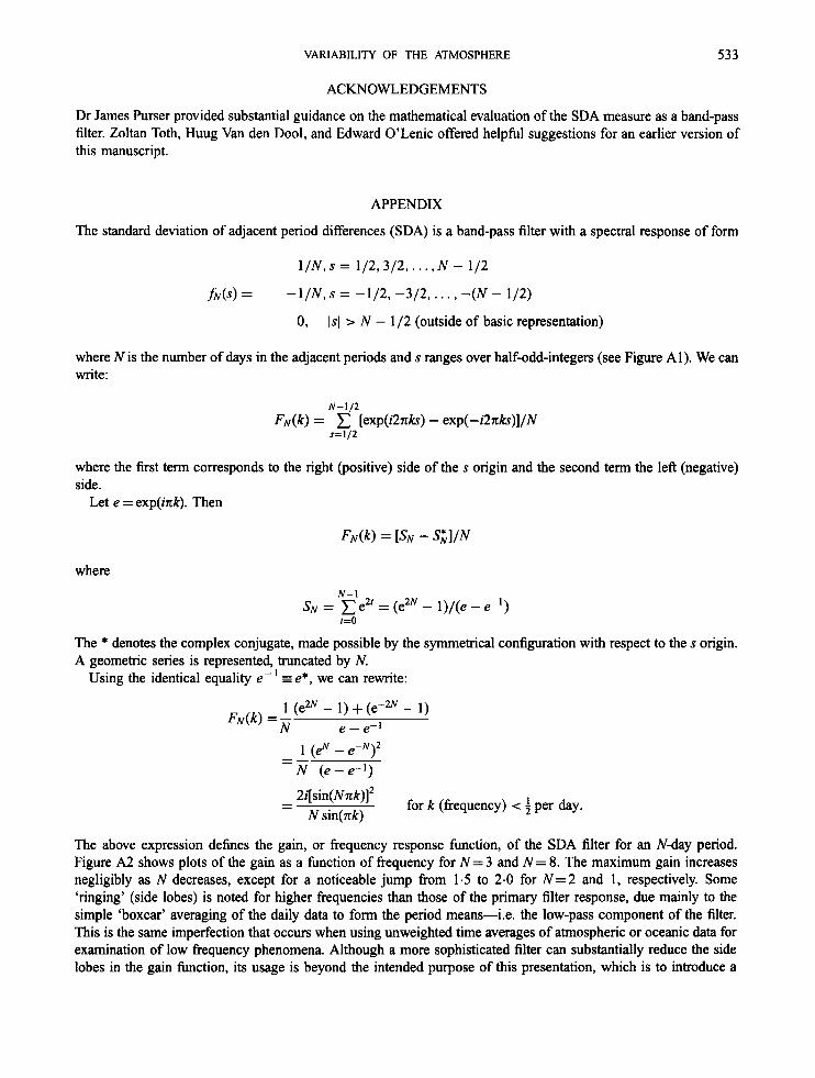
The standard deviation of adjacent period differences (SDA) is a band-pass filter with a spectral response of form

l /N , s = 1/2,3/2, . . . , N - 1/2

J;N(s) = -1/N,s = -1/2, -3/2,. . . , -(N - 1/2)

0, Is1 =- N - 1/2 (outside of basic representation)

where N is the number of days in the adjacent periods and s ranges over half-odd-integers (see Figure Al). We can write:

N - I / 2 F N ( ~ ) = [exp(i2nlrs) - exp(-i2nk)]/N

s= 1 /2

where the first term corresponds to the right (positive) side of the s origin and the second term the left (negative) side.

Let e = exp(ink). Then

where

The * denotes the complex conjugate, made possible by the symmetrical configuration with respect to the s origin. A geometric series is represented, truncated by N.

Using the identical equality e- = e*, we can rewrite:

1 (e2N - 1) + (e-2N - 1) N e - e-I

FN(k) =-

2i[sin(Nnk>l2 N sin(nk)

- - for k (frequency) < 4 per day.

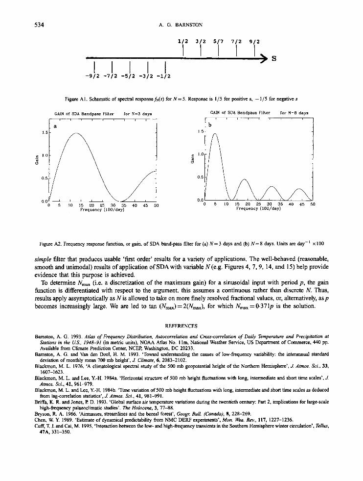
The above expression defines the gain, or frequency response function, of the SDA filter for an N-day period. Figure A2 shows plots of the gain as a function of frequency for N= 3 and N= 8. The maximum gain increases negligibly as N decreases, except for a noticeable jump from 1.5 to 2.0 for N = 2 and 1, respectively. Some ‘ringing’ (side lobes) is noted for higher frequencies than those of the primary filter response, due mainly to the simple ‘boxcar’ averaging of the daily data to form the period means-i.e. the low-pass component of the filter. This is the same imperfection that occurs when using unweighted time averages of atmospheric or oceanic data for examination of low frequency phenomena. Although a more sophisticated filter can substantially reduce the side lobes in the gain function, its usage is beyond the intended purpose of this presentation, which is to introduce a

534 A. G. BARNSTON

Figure Al. Schematic of spectral response fds) for N= 5 . Response is 1/5 for positive s, - 1/5 for negative s

GAIN of SDA Bandpass Filter for N=3 days I l I , , I , I ,

a

GAIN of SDA Bandpass Filter for N = 8 days I I I I I I , , ,

b

Figure A2. Frequency response function, or gain, of SDA band-pass filter for (a) N = 3 days and @) N= 8 days. Units are day-’ x 100

simple filter that produces usable ‘first order’ results for a variety of applications. The well-behaved (reasonable, smooth and unimodal) results of application of SDA with variable N (e.g. Figures 4,7 ,9 , 14, and 15) help provide evidence that this purpose is achieved.

To determine N,, (i.e. a discretization of the maximum gain) for a sinusoidal input with period p, the gain hc t ion is differentiated with respect to the argument. this assumes a continuous rather than discrete N. Thus, results apply assymptotically as N is allowed to take on more finely resolved fractional values, or, alternatively, asp becomes increasingly large. We are led to tan (Nm)=2(N-), for which N,,=O-371p is the solution.

REFERENCES

Bamston, A. G. 1993. Atlas of Frequency Distribution. Autocorrelation and Cross-correlation of Daily Temperature and Precipitation at Stations in the US. , 1948-91 (in metric units), NOAA Atlas No. 1 Im, National Weather Service, US Department of Commerce, 440 pp. Available from Climate Prediction Center, NCEP, Washington, DC 20233.

Barnston, A. G. and Van den Dool, H. M. 1993. ‘Toward understanding the causes of low-frequency variability: the interannual standard deviation of monthly mean 700 mb height’, 1 Climate, 6, 2083-2102.

Blackmon, M. L. 1976. ‘A climatological spectral study of the 500 mb geopotential height of the Northern Hemisphere’, 1 Amos. Sci., 33, 1 607-1 623.

Blackmon, M. L. and Lee, Y.-H. 1984a. ‘Horizontal structure of 500 mb height fluctuations with long, intermediate and short time scales’, 1 Amos. Sci., 41, 961-979.

Blackmon, M. L. and Lee, Y.-H. 1984b. ‘Time variation of 500 mb height fluctuations with long, intermediate and short time scales as deduced from lag-correlation statistics’, 1 Amos. Sci., 41, 981-991.

Briffa, K. R. and Jones, I? D. 1993. ‘Global surface air temperature variations during the twentieth cenhuy: Part 2, implications for large-scale high-frequency palaeoclimatic studies’. The Holocene, 3, 77-88.

Bryson, R. A. 1966. ‘Airmasses, streamlines and the boreal forest’, Geogr Bull. (Canada), 8, 228-269. Chen, W. Y. 1989. ‘Estimate of dynamical predictability from NMC DEW experiments’, Mon. Wea. Rev., 117, 1227-1236. Cuff, T. I. and Cai, M. 1995. ‘Interaction between the low- and high-frequency transients in the Southern Hemisphere winter circulation’, Tellus, 47A, 331-350.

VARIABILIIY OF THE ATMOSPHERE 535

Ebisuzaki, W. and Van den Dool, H. M. 1993. The Atmospheric Model Intercomparison Pmject at the National Meteomlogical Center, National

Gates, W. L. 1992. ‘AMIP: the atmospheric model intercomparison project’, Bull. Am. Meteoml. SOC., 73, 1962-1970. Kalnay, E., Kanamitsu, M., Kistler, R., Collins, W., Deaven, D., Gandin, L., Iredell, M., Saha, S., White, G., Woollen, J., Zhu, Y., Chelliah, M.,

Ebisuzaki, W., Higgins, W., Janowiak, J., Mo, K. C., Ropelewski, C., Wang, J., Leetmaa, A,, Reynolds, R., Jenne, R. and Joseph, D. 1996. ‘The NMC/NCAR 40-year reanalyses project’, Bull. Am. Meteoml. SOC., 77, in press.

Meteorological Center, Office Note No. 402, 23 pp. Available from Climate Prediction Center, NCEF‘, Washington, DC 20233.

Lorenz, E. N. 1982. ‘Atmospheric predictability experiments with a large numerical model’, Tellus, 34, 505-513. Madden, R. A. 1981. ‘A quantitative approach to long-range forecasting’, 1 Geophys. Res., 86, 9817-9825. Madden, R. A. and Shea, D. J. 1978. ‘Estimates of the natural variability of time-averaged temperatures over the United States’, Mon. Wea. Rev.,

May, W., Shea, D. J. and Madden, R. A. 1992. The Annual Variation of Surface Tempemtures over the World, National Center for Atmospheric

Saha, S. 1992. An Atlans of Monthly Mean Climatologies, Standard Dm’ations f i .m Monthly Means and Standard Deviations of Daily

Shea, D. J. 1984. The Annual Cycle, Part I: the Annual Variation of Surface Tempemture over the United States and Canada, National Center for

Toth, Z. and Szentimy, T. 1990. ‘The binormal distribution: a distribution for representing asymmetrical but normal-like weather elements’, J

Van den Dool, H. M. and Cai, M. 1994. ‘An empirical Rossby wave propagation formula’, Pmceedings ofthe International Symposium on Zhe

Van den Dool, H. M. and Saha, S. 1990. ‘Frequency dependence in forecast skill’, Mon. Wea. Rev., 118, 128-137. Van den Dool, H. M., Saha, S. and Toth, Z. 1991. ‘The climate in a multi-year Nh4C model run’, Preprints, 5th Conference on Climate

Wendland, W. M. and Bryson, R. A. 1981. ‘Northern Hemisphere airstream regions’, Mon. Wea. Rev., 109,255-270.

106, 1695-1703.

Research, Technical Note NCAR/TN-372+STR, 134 pp, Available from NCAR, PO. Box 3000, Boulder, CO 80307.

Tendencies, Available from Development Division, National Meteorological Center, Washington, DC 20233, 38 pp.

Atmospheric Research Technical Note NCAR/TN-242+STR, 77 pp. Available from NCAR, PO. Box 3000, Boulder, CO 80307.

Climate, 3, 128-236.

Life Cycler of Exrmfropical Cyclones, Bergen, Norway, 27 June to 1 July 1994, Vol. 2, pp. 9 6 9 6 .

Yariations, Denver, Colorado, American Meteorological Society, pp. 51 1-514.

Documents

TIME-SCALES OF THE VARIABILITY OF THE ATMOSPHERE