Embed Size (px)
Citation preview

This content has been downloaded from IOPscience. Please scroll down to see the full text.
Download details:
This content was downloaded by: holcman
IP Address: 129.199.23.252
This content was downloaded on 11/04/2014 at 16:50
Please note that terms and conditions apply.
Time scale of diffusion in molecular and cellular biology
View the table of contents for this issue, or go to the journal homepage for more
2014 J. Phys. A: Math. Theor. 47 173001
(http://iopscience.iop.org/1751-8121/47/17/173001)
Home Search Collections Journals About Contact us My IOPscience

Journal of Physics A: Mathematical and Theoretical
J. Phys. A: Math. Theor. 47 (2014) 173001 (50pp) doi:10.1088/1751-8113/47/17/173001
Topical Review
Time scale of diffusion in molecular andcellular biology
D Holcman1 and Z Schuss2
1 Group of Applied Mathematics and Computational Biology, IBENS,Ecole Normale Superieure, 46 rue d’Ulm, F-75005 Paris, France2 Department of Applied Mathematics, Tel-Aviv University, Tel-Aviv 69978, Israel
E-mail: [email protected] and [email protected]
Received 25 July 2013, revised 14 February 2014Accepted for publication 17 February 2014Published 9 April 2014
AbstractDiffusion is the driver of critical biological processes in cellular and molecularbiology. The diverse temporal scales of cellular function are determined byvastly diverse spatial scales in most biophysical processes. The latter are due,among others, to small binding sites inside or on the cell membrane or tonarrow passages between large cellular compartments. The great disparity inscales is at the root of the difficulty in quantifying cell function from moleculardynamics and from simulations. The coarse-grained time scale of cellularfunction is determined from molecular diffusion by the mean first passagetime of molecular Brownian motion to a small targets or through narrowpassages. The narrow escape theory (NET) concerns this issue. The NET isubiquitous in molecular and cellular biology and is manifested, among others,in chemical reactions, in the calculation of the effective diffusion coefficientof receptors diffusing on a neuronal cell membrane strewn with obstacles, inthe quantification of the early steps of viral trafficking, in the regulation ofdiffusion between the mother and daughter cells during cell division, and manyother cases. Brownian trajectories can represent the motion of a molecule,a protein, an ion in solution, a receptor in a cell or on its membrane, andmany other biochemical processes. The small target can represent a bindingsite or an ionic channel, a hidden active site embedded in a complex proteinstructure, a receptor for a neurotransmitter on the membrane of a neuron, andso on. The mean time to attach to a receptor or activator determines diffusionfluxes that are key regulators of cell function. This review describes physicalmodels of various subcellular microdomains, in which the NET coarse-grainsthe molecular scale to a higher cellular-level, thus clarifying the role of cellgeometry in determining subcellular function.
1751-8113/14/173001+50$33.00 © 2014 IOP Publishing Ltd Printed in the UK 1

J. Phys. A: Math. Theor. 47 (2014) 173001 Topical Review
Keywords: stochastic modeling, diffusion, asymptotic methods, Fokker–Planckequation, flux regulation, molecular trafficking, molecular biophysicsPACS numbers: 82.20.Uv, 82.39.−k, 02.30.Jr, 87.10.Ed, 02.50.Ga, 87.18.Sn,87.19.lg, 82.20.−w, 02.50.Fz, 87.10.Mn
(Some figures may appear in colour only in the online journal)
Contents
1. Introduction 21.1. References to section 1 5
2. Theory of stochastic chemical reactions in confined microdomains 62.1. Flux regulation by receptor clustering in cellular biology 82.2. Random search with switching between different states 92.3. References to section 2 15
3. Diffusion on a crowded membrane and intracellular trafficking 163.1. Diffusion on a membrane crowded with obstacles 173.2. Trafficking and the delivery flux of vesicles in neurite outgrowth 203.3. References to section 3 20
4. Physical virology: modeling the early steps of cell viral infection at the molecular level 214.1. The cytoplasmic viral trafficking 214.2. Stochastic description of viral trajectories 214.3. Probability that a viral particle arrives alive at a nuclear pore 254.4. The mean arrival time to a small nuclear pore 264.5. Endosomal viral escape 264.6. References to section 4 27
5. The NET in neurobiology and synaptic transmission 275.1. A model of the synaptic current 295.2. The mean and variance of the synaptic current Is 305.3. Leakage in a conductor of Brownian particles 325.4. Regulation of flux in a neuronal spine neck and across a thin synaptic cleft 345.5. References to section 5 37
6. Diffusion in composite domains 386.1. Transition rate and the principal eigenvalue in composite domains 416.2. The principal eigenvalue in a domain with a head and narrow neck 426.3. The principal eigenvalue and coarse-grained diffusion in a dumbbell 436.4. Diffusional transfer of genetic material during cell division 44
7. Summary and discussion 45Acknowledgment 45References 45
1. Introduction
Diffusion drives critical biological processes in cellular physiology, such as the search for abinding partner in biochemistry, the neuronal transmission in neurophysiology (Kandel et al2000, Alberts et al 1994), the splitting of molecules (mRNA or proteins) between motherand daughter cells during cell division, and many other processes. The very different spatialand temporal scales in these processes are due to small binding sites inside or on the cell
2

J. Phys. A: Math. Theor. 47 (2014) 173001 Topical Review
boundary, or narrow passages between large compartments. The great disparity in scales inthese examples is manifested as singular perturbation problems in their mathematical models.The quantification of the function of cellular microdomains from their geometrical structure,such as of neuronal synapses, falls in the class of multiple-scale problems of narrow escapetheory (NET) (Holcman and Schuss 2014). The narrow escape time NET in diffusion theoryis the mean first passage time (MFPT) of a Brownian trajectory to a small absorbing part of anotherwise reflecting boundary of a bounded domain. The renewed interest in the NET is dueto its emergence as a key to the determination of biological cell function from its geometricalstructure.
The physics of cell function has to be understood at the molecular level, which determinesthe dynamics of much larger cellular structures, such as the dynamics of molecular fluxes inmicrodomains and synapses (figure 14). Physical modeling on the cellular scale has seriouspitfalls, because the temporal scale of cellular events is determined on the molecular levelby refined details of cell structure, which cannot be captured in cellular-level models. Thistime scale has to be divined from a much lower-level model (see references in section 1.1).The behavior of molecules is complex not only because of their individual structure, but alsobecause they form clusters or have specific interactions (see section 2.1).
Brownian dynamics simulations of molecular models often fail to capture the time scale ofrare events, such as the passage of ions through protein channels of cellular membranes or thepassage of molecules through narrow passages between cellular compartments. An analyticalapproach to the evaluation of the rate of rare events can lead to rational coarse-grainingof the molecular model. For example, the analytical expression for the NET (Holcman andSchuss 2014) reduces the dimension of stochastic simulation data of exploration to that ofthe parameter space of the dynamics. It leads to an analytical expressions for an effectivediffusion coefficient and for the rate of passage between compartments through necks. Thenarrow passage is especially important in quantifying the molecular searches that are notdirected at long distances by a field of force and the only flux-control mechanism is thegeometrical structure.
The development of molecular-level models follows a recent technological development oflive-cell microscopy, which affords access to individual molecular trajectories on the surface ofneuronal cells (Choquet and Borgdorff 2002, Borgdorff and Choquet 2002, Triller and Choquet2003). Marked molecules provide short-time samples of trajectories that can be traced (Hozeet al 2010), therefore the reconstruction of their dynamics from the statistics of the samplesis not an obvious task. The Brownian trajectories of the marked molecules cannot penetratethe cell membrane or other obstacles, but can be absorbed at receptors and other binding sites,or be terminated by a change of conformation or other chemical reactions, or when they exitthe cell or a subcellular compartment and enter another structure. Different compartments forBrownian trajectories are often defined by the probability density of the observed trajectoriesor by the statistics of the time trajectories spend in a given spatial domain. By its very definition,the passage of a trajectory from one compartment to another is a rare event, which may bethermal activation over a potential barrier and/or (Holcman and Schuss 2004) traversing anarrow passage (Holcman and Schuss 2011), such as a channel, a single-file nano-pore, or anarrow neck.
Singular perturbation methods for the asymptotic analysis of the NET problem arereviewed in Holcman and Schuss (2014), where explicit expressions for NET are given.Approximate analytical and numerical solutions of the associated boundary value problemsfor the Pontryagin–Andronov–Vitt equation (Schuss 2010b, 2013) are derived for variousgeometries representing accessible and hidden single or multiple targets. The asymptoticmethods are based on solving mixed Dirichlet–Neumann problems for elliptic and parabolic
3

J. Phys. A: Math. Theor. 47 (2014) 173001 Topical Review
Figure 1. Brownian trajectory escaping through a small absorbing window of a domainwith otherwise reflecting boundary.
equations using the singularity of the Neumann function (Singer et al 2008). The NET is alsoshown to be related to the principal eigenvalue of the mixed Dirichlet–Neumann problem forthe Laplace equation in a domain, when the Dirichlet boundary is only a small patch on theotherwise Neumann boundary. As mentioned above, the principal eigenvalue is asymptoticallythe reciprocal of the NET in the limit of shrinking Dirichlet patch. In this limit the escape ofa Brownian trajectory becomes a rare event and is thus hard to track by Brownian dynamicssimulations due to the high computational complexity and to the high dimension of theparameter space. The explicit asymptotic approximation for the NET leads to the design ofBrownian simulations of cellular processes, as described below. This review explains howto use these expressions to coarse-grain biophysical and biological models and to extractproperties from newly available molecular data and from Brownian simulations.
The NET τ , that is, the MFPT of a Brownian trajectory from a compartment to an absorbingtarget (figure 1) or through a narrow passage, is a fundamental concept in the description ofrare events. Specifically, in the limit of small target τ increases indefinitely and the probabilitydensity function of the time spent in a compartment prior to termination or escape becomesexponentially distributed (Schuss et al 2007, Schuss 2010b, section 6.1)
pτ (t) ∼ τ−1 exp{−t/τ }. (1.1)
The exponential rate τ−1 is therefore the flux into the absorbing target. In the case of crossingfrom one compartment to another through a narrow neck the crossing rate is 1/2τ , where τ isthe MFPT to the stochastic separatrix (SS) between the compartments, the latter is the locusof initial points of a Brownian trajectory from which it ends up in one compartment or theother with equal probabilities (Schuss 2010a). The rate can represent the molecular flux intoreceptors or through intercellular passages, such as channels or necks and therefore determinescell functions, such as neuronal signaling and other key cell functions. The importance of theexplicit computation of τ in a given model consists in the drastic reduction in the dimensionof Brownian dynamics simulations to that of the dimension of the parameter space of theanalytical expression for the NET. This reduction coarse-grains molecular physical modelsinto the micrometer scale of cellular or subcellular structure and function.
When the moving particle is initially positioned close to the target (inside the boundarylayer), escape is characterized by the probability distribution of arrival times and not simply bythe exponential tail of the distribution (Mattos et al 2012). In dimension two, the boundary layer
4
J. Phys. A: Math. Theor. 47 (2014) 173001 Topical Review
expansion can be computed explicitly (Singer et al 2006a), whereas short-time asymptoticsare much harder to estimate (see, for example, the short-time asymptotics given in Schuss andSpivak (2005) for pure diffusion), because they requires the knowledge of all the eigenvaluesof the problem. The full probability distribution of arrival times can be evaluated by heavynumerical simulations.
There are several examples where an anomalous diffusion model is needed to describemore refined properties of molecular motion. This is the case for the motion of a singlemonomer on a polymer chain (Amitai 2010, Amitai and Holcman 2013). In other cases,the size of a diffusing particle affects its motion (Barkai et al 2012), (see also experimentalevidences in Tabei et al (2012) and Jeon et al (2011)). We refer to other reviews for specificdiscussion of anomalous diffusion (Hoefling and Franosch 2013).
This review presents several molecular and cellular, as well as biophysical models, whichare based on the NET approximation. In this approximation the details of the geometricalstructure are coarse-grained into single parameter, the reciprocal of the NET, which is thearrival rate at a small absorbing boundary. Recent progress is reported on coarse-grainingmolecular-level models to cellular scale and on their resolution. The coarse-grained modelsextract cell function from the cell’s geometrical structure. The first section presents a theory ofstochastic chemical reactions in confined microdomains, based on a Markov chain model. Inthis theory the mean by which a given number of binding sites are activated can be calculated.It also presents the search strategy of a Brownian particle that switches at random betweentwo states, but can find a small target only when in one of the two. Section two presents amodel for computing the effective diffusion coefficient on a membrane crowded with obstaclesand some applications to receptor trafficking on the surface of a neuron. Section 3 presentsseveral models for the molecular-level study of the successive steps of viral infection insidea cell. The mathematical model for the study of the mean escape time of a virus from anendosome uses stochastic dynamics to describe cytoplasmic trafficking and Markov jumps.The model defines the probability of a virus arrival at the nucleus in terms of the Fokker–Planck equation. The success of the early steps of viral trafficking determine the capacity forviral infection (Amoruso et al 2011). Section 4 presents several diffusion problems related tosynaptic transmission that take place at the junction between two neurons (Cowan et al 2003,Kandel et al 2000). An asymptotic computation is shown of the probability that a receptorin the synaptic cleft binds a diffusing neurotransmitter (NT) (figure 14). A summary is givenof diffusion laws inside composite domains, such as dendritic spines, which are fundamentalmicrodomains in synaptic communication (figure 20). The laws are based on flux formulasthat are also used in the context of diffusion between cells. Finally, a discussion is given ofpossible extensions of the NET methodology to other molecular and cellular questions.
1.1. References to section 1
The narrow escape problem in diffusion theory was considered first by Lord Rayleighin Rayleigh (1945) and elaborated in Fabrikant (1989), 1991); the terminology NET wasintroduced in Singer et al (2006c). A recent review of early results on the NET problemwith many biological applications is given in Bressloff and Newby (2013). A basic text onneuroscience is Kandel et al (2000), where the terminology used in this section is explained.The neuronal cleft is discussed in Alberts et al (1994, chapter 19) and Kandel et al (2000).The description of ionic channels, their selectivity, gating, and function is given in Sakmannnand Neher (2010) and Hille (2001) (see also the Nobel lecture (MacKinnon 2003)). Thereconstruction of the spatial organization of proteins and ions that define the channel pore
5

J. Phys. A: Math. Theor. 47 (2014) 173001 Topical Review
from recordings of channel current–voltage characteristics is described in Chen et al (1997)and Burger et al (2007).
2. Theory of stochastic chemical reactions in confined microdomains
The need to simulate several interacting species in a microdomain is particularly useful inthe context of calcium dynamics in neuronal synapses. The number of involved moleculesis of the order of tens to hundreds, which are tracked with fluorescent dyes that drasticallyinterfere with the reaction and diffusion processes. A similar situation arises in the simulationof synaptic transmission, starting with the arrival of NT molecules at receptors on the post-synaptic membrane.
A significant reduction of the simulation complexity is achieved by using the analyticallycomputed neurotransmitter flux into the receptors, rather than simulating it. Analyticalformulas are also used for quantifying diffusion in dendritic spines. Additional progressin modeling chemical reactions is achieved by replacing complex Brownian simulations withcoarse-grained Markov chains by taking advantage of the fact that the arrival process ofBrownian particles from a practically infinite continuum to an absorbing target is Poissonian.It is possible then to coarse-grain the binding and unbinding processes in microdomains intoa Markov process, thus opening the way to full analysis of stochastic chemical reactions.This simulation circumvents the complex reaction–diffusion partial differential equations thatare much harder to solve. A recent application of this Markovian approximation concernssome new predictions about the rate of molecular dynamics that underlie the spindle assemblycheckpoint during cell division. Another reduction achieved by using the asymptotic analyticalapproximation to the NET is the verification of molecular dynamics simulations in domainsthat contain small passages or targets. The convergence of the simulation can be measured bythe convergence of the statistics of rare events to that predicted by the analytical asymptoticapproximation.
Traditional chemical kinetics, based on mass-action laws or reaction–diffusion equations,give an inappropriate description of the stochastic chemical reactions in microdomains, whereonly a small number of substrate and reactant molecules is involved. A reduced Markoviandescription of the stochastic dynamics of the binding and unbinding of molecules is given inHolcman and Schuss (2005) and applied in Dao Duc and Holcman (2010, 2012). Specifically,consider two finite species, the mobile reactant M that diffuses in a bounded domain � andthe stationary substrate S (e.g., a protein) that binds M. The boundary ∂� of the domain � ispartitioned into an absorbing part ∂�a (e.g., pumps, exchangers, another substrate that formspermanent bonds with M, and so on) and a reflecting part ∂�r (e.g., a cell membrane). In thismodel the volume of M is neglected. In terms of traditional chemical kinetics the binding ofM to S follows the law
M + Sfree
k f
�kb
MS, (2.1)
where k f is the forward binding rate constant, kb is the backward binding rate constant, andSfree is the unbound substrate. The model of the reaction assumes that the M molecules diffusein � independently and when bound, are released independently of each other at exponentialwaiting times with rate k−1.
To calculate the average number of unbound (or bound) sites in the steady statethe following reduced model is used. The number k(t) of unbound receptors at time tis a Markovian birth–death process with states 0, 1, 2, . . . , min{M, S} and transition rates
6

J. Phys. A: Math. Theor. 47 (2014) 173001 Topical Review
λk→k+1 = λk, λk→k−1 = μ = k−1. The boundary conditions are λS→S+1 = 0 andλ0→−1 = 0. Setting Pk(t) = Pr{k(t) = k}, the Kolmogorov equations for the transitionprobabilities are given by Holcman and Schuss (2005)
Pk(t) = −[λk + k−1(S − k)]Pk(t) + λk+1Pk+1(t) + k−1(S − k + 1)Pk−1(t) (2.2)
for k = (S − M)+ + 1, . . . , S − 1
with the boundary equations
P(S−M)+ (t) = −k−1SP(S−M)+ (t) + λ1P(S−M)++1(t)
PS(t) = −λSPS(t) + k−1PS−1(t)
and initial condition Pk,q(0) = δk,Sδq,0. In the limit t → ∞ the model (2.2) gives the averagenumber
〈k∞〉 =S∑
j=(S−M)+jPj,
where Pj = limt→∞ Pj(t). Similarly, the stationary variance of the number of unbound sites is
σ 2(M, S) = 〈k2∞〉 − 〈k∞〉2, where 〈k2
∞〉 = ∑Sj=(S−M)+ j2Pj.
The rates λk are modeled as follows. For a single diffusing molecule, the time to bindingis the first passage time to reach a small absorbing portion ∂�a of the boundary, whichrepresents the active surface of the receptor, whereas the remaining part of ∂� is reflecting.Due to the small target and to the deep binding potential well the binding and unbinding ofM to S are rare events on the time scale of diffusion (Schuss et al 2007). This implies that theprobability distribution of binding times is approximately exponential (Schuss 2010b) withrate λ1 = 1/Eτ1, where the NET Eτ1 is the MFPT to ∂�a. When there are S binding sites,k(t) of which are unbound, there are N = [M − S + k]+ free diffusing molecules in �, wherex+ = max{0, x}. The arrival time of a molecule to the next unbound site is well approximatedby an exponential law with state-dependent instantaneous rate (see discussion in Holcman andSchuss 2005)
λk = Nk
Eτ1= k(M − S + k)+
Eτ1.
The results of the Markovian model (2.2) are
PS = 1
1 + ∑S−(S−M)+k=1
∏Si=S−k+1 i(M−S+i)+
k!(Eτ1k−1)k
〈k∞〉 = PS
(S−M)+∑k=S−1
(S − k)+∏S
i=S−k+1 i(M − S + i)+
k!(Eτ1k−1)k
〈k2∞〉 = PS
(S−M)+∑k=S−1
[(S − k)+]2
∏Si=S−k+1 i(M − S + i)+
k!(Eτ1k−1)k
σ 2S (M) = 〈k2
∞〉 − 〈k∞〉2 (2.3)
(see Holcman and Schuss (2005) for further details).These formulas are used to estimate the fraction of bound receptors in photo-receptor
outer segments and also to interpret the channel noise measurements variance in Holcman andSchuss (2005). In Holcman and Triller (2006) this analysis was used to estimate the number ofbound AMPA receptors in the post-synaptic density (PSD). A similar gated Markovian modelwas proposed in Bressloff and Earnshaw (2009). The reduced Markovian model is used for the
7
J. Phys. A: Math. Theor. 47 (2014) 173001 Topical Review
calculation of the mean time of the number of bound molecules to reach a given threshold T(MFTT). In a cellular context, the MFTT can be used to characterize the stability of chemicalprocesses, especially when they underlie a biological function. Using the above Markov chaindescription, the MFTT can be expressed in terms of fundamental parameters, such as thenumber of molecules, of ligands, and the forward and backward binding rates. It turns outthat the MFTT depends nonlinearly on the threshold T . Specifically, consider M Brownianmolecules that can bind to immobile targets S inside a microdomain, modeled genericallyby equation (2.1). The first time the number [MS](t) of MS molecules at time t reaches thethreshold is defined as
τT = inf{t > 0 : [MS](t) = T } (2.4)
and its expected value is τT . Consider the case of an ensemble of the targets initially freeand distributed on the surface of a closed microdomain and assume that the backward ratevanishes (k−1 = 0) and k f > 0. The dynamical system for the transition probabilities ofthe Markov process MS(t) is similar to that above, but for the absorbing boundary conditionat the threshold T , which gives (2.2) (Dao Duc and Holcman 2010). When the binding isirreversible (k−1 = 0), τT is the sum of the forward rates
τ irrevT = 1
λ0+ 1
λ1+ · · · + 1
λT−1
= 1
λ
T−1∑k=0
1
(M0 − k)(S0 − k). (2.5)
In particular, when M0 = S0 and M0 � 1, (2.5) becomes asymptotically τ irrevT ≈
T/λM0(M0 − T ). In addition, when the number of diffusing molecules largely exceed thenumber of targets (M0 � S0, T ), (2.5) gives the asymptotic formulas
τ irrevT ≈
⎧⎪⎪⎪⎪⎪⎪⎪⎪⎪⎨⎪⎪⎪⎪⎪⎪⎪⎪⎪⎩
1
λM0log
S0
S0 − Tfor M0 � S0, T
1
λS0log
M0
M0 − Tfor S0 � M0, T
T
λM0S0for M0, S0 � T.
(2.6)
Figure 2 shows the plot of τ irrevT for several values of the threshold T , compared to Brownian
simulations in a circular disk � = D(R) with reflecting boundary, except at the targets.
2.1. Flux regulation by receptor clustering in cellular biology
There are several studied examples, where changing the arrangement of absorbing windowsaffects the cell function. In bacteria, receptors re-cluster, depending on the externalconcentration of a chemotactic attractant, thus improving the sensitivity. In the context ofneuroscience, receptors are known to re-cluster before the tip of a growing neuron (growthcone) turns toward a chemoattractant. Changing the arrangement of AMPA receptors inneuronal synapses affects the synaptic transmission. The variations in the shape of dendriticspines of neurons as a result of learning and other physiological activities changes boththe density and distribution of receptors, transporters and other regulatory proteins, therebychanging the ionic flux through the membrane. Thus calcium dynamics in dendritic spines canbe controlled at the cellular level by rearrangement of channels and exchangers.
8

J. Phys. A: Math. Theor. 47 (2014) 173001 Topical Review
−1 −0.5 0 0.5 1−1
−0.8
−0.6
−0.4
−0.2
0
0.2
0.4
0.6
0.8
1
4 5 6 7 8 9 10 110
5
10
15
20
25
30
35
T (Threshold)
Figure 2. The MFTT. Left: trajectories of diffusing molecules in a microdomaincontaining five binding sites on the boundary. Right: the time τ irrev
T is plotted as afunction of the threshold T . Brownian simulations (dotted blue line, variance in black),the theoretical formula (2.5) (dotted red line) and its approximation (2.6) (continuousblue line) for a circular disk in the irreversible case (k−1 = 0). The other parameters areS0 = 15, M0 = 10 , ε = 0.05 , D = 0.1 μm2s−1 and the radius of the disk R = 1 μm(200 runs).
Ω
∂Ωa
∂Ωr
x
Figure 3. Example of a trajectory of a diffusing Brownian ligand in a confined domain� and randomly switching between two states 1 (continuous line) and 2 (dashed line).In state 2, the ligand is reflected all over the boundary, while in state 1 it is absorbed at∂�a.
2.2. Random search with switching between different states
Consider Brownian motion in a bounded domain �, whose diffusion coefficient is a randomtelegraph signal that switches between two values, D1 and D2, at exponential waiting timeswith rates k12 and k21, respectively (see figure 3). When the diffusion coefficient is D1, theBrownian trajectory is reflected in the boundary ∂�, except for a small absorbing part ∂�a.When the diffusion coefficient is D2, the entire boundary reflects the Brownian trajectory.The gated narrow escape time (GNET) is the time to absorption of the switching Browniantrajectory and the mean time to absorption is the GNET. More generally, a class of diffusionsis considered that switch between different diffusion coefficients D1, . . . , Dn at exponentialwaiting times with given rates ki j and are absorbed at a small part ∂�a of ∂� while in statesD1, . . . , Dk and are otherwise reflected in ∂�. The GNET is related to certain intermittent
9

J. Phys. A: Math. Theor. 47 (2014) 173001 Topical Review
search processes, where switching strategies between different states lead to minimal searchtime of a target (Benichou et al 2005). Other switching searches have been investigated wherea stochastic particle moves close to the surface membrane (Tsaneva et al 2009, Oshanin et al2010, Berezhkovskii and Barzykin 2012).
The gated narrow escape model is used to calculate the GNET, which requires the solutionof a coupled system of mixed Dirichlet–Neumann boundary value problems for Poisson’sequations. The system was recently solved in Reingruber and Holcman (2009, 2010).
2.2.1. Random switching between two modes of diffusion. Consider stochastic dynamicsx(t, i) that switches between two states, i = 1 and i = 2 (e.g., due to change of conformation),at exponential waiting times with rates k12 and k21, respectively, and diffuses in state i withdiffusion constant Di. Its Euler simulation for t > s is given by
x(t + t, i) =⎧⎨⎩
x(t, i) + √2Diwi(t) w.p. 1 − ki jt + o(t)
x(t, j) w.p. k jit + o(t), i = j(2.7)
for i, j = 1, 2, with an initial condition x(s, i) = x, in which the states i = 1 and i = 2 can berandomly distributed. Here wi(t) (i = 1, 2) are independent standard Brownian motions andwi(t) = wi(t + t) − wi(t).
The transition probability density function p(y, i, t | x, s, j) of the trajectory x(t, i) in agiven domain �, given the initial condition x(s, j) = x with probability 1, is the limit ast → 0 of the solution to the system of integral equations (Schuss 2010b)
p(y, i, t + t | x, s, j) = 1 − ki jt√2πDit
∫�
p(z, i, t | x, s, j) exp
{−|y − z|2
2Dit
}dz
+ k jit p(y, �, t | s, j) + o(t) for i, j, � = 1, 2, i = �.
In the limit t → 0, the system of Kolmogorov (master) equations is obtained
pt (y, 1, t | x, s) = D1y p(y, 1, t | x, s) − k12 p(y, 1, t | x, s) + k12 p(y, 2, t | x, s)
pt (y, 2, t | x, s) = D2y p(y, 2, t | x, s) + k21 p(y, 1, t | x, s) − k21 p(y, 2, t | x, s), (2.8)
which can be easily generalized to any number of states (Reingruber and Holcman 2010).Setting
p =(
p(y, 1, t | x, s)p(y, 2, t | x, s)
), K =
(k12 −k12
−k21 k21
), Dy =
(D1 00 D2
)y,
the forward master equations (2.8) can be written as
pt (y, t | x, s) = Dy p(y, t | x, s) − Kp(y, t | x, s). (2.9)
The transition probability density function p (y, t | x, s) satisfies the backward system of masterequations (with respect to (x, s)), which is the formal adjoint to (2.9). Upon setting t − s = τ ,as we may, we obtain
pτ (y, τ | x, 0) = Dx p(y, τ | x, 0) − KT p(y, τ | x, 0). (2.10)
The mean sojourn time in state i prior to absorption, u(i |x, 1), of a trajectory of (2.7) thatstarts at τ = 0 in state 1 at position x with probability 1, is given by Schuss (2010b)
u(i | x, 1) =∫
�
dy∫ ∞
0dτ p(y, i, τ | x, 1). (2.11)
To find the differential equations that the times u(i |x, j) satisfy, the backward equation (2.10)is integrated with respect to y and τ to obtain
D1u(i | x, 1) − k12[u(i | x, 1) − u(i | x, 2)] = −1
D2u(i | x, 2) − k21[u(i | x, 2) − u(i | x, 1)] = 0.
10
J. Phys. A: Math. Theor. 47 (2014) 173001 Topical Review
The mean sojourn times u(2 | x, 1) and u(2 | x, 2) satisfy equations that are obtained byinterchanging 1 ↔ 2 in (2.12). It suffices to solve the equations only for i = 1, because thesolutions u(2 | x, j) can be obtained from u(1 | x, j) by linear transformations. Specifically,averaging u(i | x, j) over a uniform initial spatial distribution of x, we define the mean sojourntimes prior to absorption as
u(i | j) = 1
|�|∫
�
u(i | x, j) dx. (2.13)
When the trajectory x(t, i) is absorbed at ∂�a with i = 1 while it is reflected everywhere onthe ∂� with i = 2, the boundary conditions for the system (2.12) are
u(1 | x, 1) = 0 for x ∈ ∂�a,∂u(1 | x, 1)
∂n= 0 for x ∈ ∂�r,
∂u(1 | x, 2)
∂n= 0 for x ∈ ∂�.
The sojourn times u(2 | x, 1) and u(2 | x, 2) are obtained from u(1 | x, 1) and u(1 | x, 2) throughthe linear transformation(
u(2 | x, 1)
u(2 | x, 2)
)= k12
k21
(1 00 1
)(u(1 | x, 1)
u(1 | x, 2)
)+
(0
1/k21
). (2.14)
Equations (2.12) and (2.14) show that the spatially averaged sojourn times (2.13) satisfy therelations
u(1 | 2) = u(1 | 1), u(2 | 1) = u(1 | 1)k12
k21, u(2 | 2) = u(2 | 1) + 1
k21. (2.15)
It follows that the mean sojourn times u(1), u(2), and u, conditioned on a uniform initialdistribution in states 1, 2, or in 1 and 2 with the equilibrium distribution (p1, p2) =(k21, k12)/(k12 + k21), respectively, are
u(1) = u(1 | 1) + u(2 | 1) = u(1 | 1)
(1 + k12
k21
)
u(2) = u(2 | 2) + u(2) = u(1) + 1
k21(2.16)
u = p1u(1) + p2u(1 | 2) = u(1) + p2
k21.
2.2.2. GNET in one dimension. The GNET for one-dimensional diffusion, though notdirectly relevant to biological applications, can be calculated explicitly (Reingruber andHolcman 2009, 2010) and is quite instructive about the dependence of the NET on switching.Specifically, the system (2.12) in the interval � = (0, L) with absorption at x = 0 in state 1and reflection at x = L is given in the scaled variables
x = x
L, l1 = k12L2
D1, l2 = k21L2
D2(2.17)
κ = D1
D2, v1(x) = D1
L2u1(x, 1), v2(x) = D1
L2u1(x, 2)
by
v′′1 (x) − l1[v1(x) − v2(x)] = −1, v′′
2 (x) + l2[v1(x) − v2(x)] = 0, (2.18)
11

J. Phys. A: Math. Theor. 47 (2014) 173001 Topical Review
0 50 1000
0.2
0.4
0.6
1
l1
u1(1)τ1
l2 = 1l2 = 10l2 = 100
0 50 1000
0.2
0.4
0.6
0.8
1
l2
l1 = 5l1 = 10l1 = 100
Figure 4. Graph of the sojourn time u(1 | 1) obtained from the explicit solution as afunction of l1 (left) and l2 (right), scaled by the NET τ1 with no switching. The continuouscurve in the left panel is the asymptotic approximation 3/
√l1 for l1 � 1 and
√l1 � l2.
with boundary conditions v1(0) = v′1(1) = v′
2(0) = v′2(1) = 0, which can be solved
explicitly. The nonlinear effect of switching can be seen from the explicit expressions
u(1 | 1) =
⎧⎪⎪⎪⎪⎨⎪⎪⎪⎪⎩
L2
D1
[coth
√l1√
l1− 1
l1
]+ O
(l2l1
), for l2 � l1
L2
3D1+ O
(l1l2
), for l2 � l1,
(2.19)
while for l1 � 1 and l2 � √l1
u(1 | 1) ≈ L2
D1
1√l1
= L√k12D1
, l1 � 1,√
l1 � l2. (2.20)
Figure 4 shows the plots of u(1 | 1) versus l1 (left) and versus l2 (right). The counterintuitiveresult, that the sojourn time u(1 | 1) is always smaller than the mean exit time in state 1 withoutswitching, is remarkable. In addition, when the parameters D1, D2, and k21 are fixed, (2.20)shows that u(1 | 1) becomes arbitrarily small as k12 increases. This counter intuitive behaviorcan be understood as follows (see also Doering (2000)). For a trajectory starting uniformlydistributed in state 1, the probability to be in the neighborhood of the absorbing boundaryat x = 0 decreases quickly as a function of time. However, after switching to state 2, thedistribution is re-homogenized and later on, after switching back to state 1, the probabilitydensity around x = 0 is higher than that in the non-switching case. After switching back tostate 1, the ligand starts closer to x = 0 with high probability and thus exits in state 1 fasterthan in the non-switching case. Figure 5 (left) shows the plot of u(1) versus l1 for various fixedvalues of l2. This situation describes a chemical reaction, where the diffusion constants andthe backward rate k21 are fixed, but the forward binding rate k12 can be adjusted by changingthe concentration of a reactant partner. Figure 5 (right) shows the plot of u(1) versus l2 forfixed l1, which demonstrates that also u(1) has a minimum u(1)m in this case. The minimumu(1)m decreases as switching becomes faster. A lower bound for u(1)m can also be foundexplicitly. The analysis of the one-dimensional case shows that the lower limit of the GNETu(1) corresponds to diffusion with the maximal diffusion constant and for κ = D1/D2 � 1,the fastest exit is achieved by diffusing most of the time in state 2, with no exits possible. Theexit time u(1) has no global or even local minima for κ < 1 and the best strategy to minimizethe GNET needs to be adapted to the given constraints. For example, when k21 k12 are theunbinding and the binding rates, respectively, k21 usually depends on the local interaction
12

J. Phys. A: Math. Theor. 47 (2014) 173001 Topical Review
0 2000 4000 60000
0.5
1
1.5
l1
u(1)τ1
l2 = 20l2 = 40l2 = 100
0 50 100
0.5
1
1.5
2
l2
l1 = 5l1 = 10l1 = 100
Figure 5. Graph of the exit time u(1) as a function of l1 (left) and l2 (right) forD1/D2 = 0.1, scaled by NET τ1 in the absence of switching.
potential while k12 can be modulated by changing the concentration of the binding partner.Furthermore, as shown in figure 5, the graph of u(1) around and past the minimum is quiteflat, and thus increasing switching to attain the minimum may not be necessary, because asimilar effect can already by achieved at much slower rates. Moreover, because the graph ofu(1) decays steeply for small values l1 and l2, this behavior provides an efficient mechanismto modulate the activation time, and thus modulate cellular signaling.
2.2.3. GNET in three dimensions. Consider the GNET problem for a three-dimensionaldomain � when the trajectory is absorbed upon hitting ∂�a in state 1 only. In the absenceof switching, the time reduces to the NET τ1 (Kolokolnikov et al 2005, Singer et al 2006b,Grigoriev et al 2002), which shows that outside a small boundary layer around the absorbinghole of radius a, where a characterizes the extent of ∂�a, the positional NET is almostindependent of the initial ligand position (Singer et al 2006b). Using the scaling (Reingruberet al 2009)
x = xa, l1 = k12a2
D1, l2 = k21a2
D2, v1(x) = aD1
|�| u1(x, 1), v2(x) = aD1
|�| u1(x, 2),
the equations (2.12) become the dimensionless system
v(i|x, 1) − l1[v(i | x, 1) − v(i | x, 2)] = −|�|−1
v(i | x, 2) + l2[v(i | x, 1) − v(i | x, 2)] = 0,(2.21)
where |�| = |�|/a3 � 1. The boundary conditions are absorbing on ∂�a for v1(x), andotherwise reflecting. Asymptotic approximations to the solution of (2.21) in the limit ofsmall window and extreme values of the parameters clarify the effect of switching. Forl1 � 1 or l2 � l1, at leading orders, v(1 | x, 1) is the solution of the NET problemv(1 | x, 1) = −|�|−1. When l2 � √
l1, the leading order approximation for v(1 | x, 1)
is found by solving v(1 | x, 1) − l1[v(1 | x, 1) − v1] = −|�|−1, where v1 is the spatialaverage of v(1 | x, 1). The leading order asymptotic approximation to the mean sojourn timeis
u(1) =(
1 + k12
k21
) |�|aD1
v1 (2.22)
∼(
1 + k12
k21
)⎧⎨⎩
τ1 for l1 � 1 or l2 � l1|�|
|∂�a|√
D1k12for l1 � 1,
√l1 � l2,
(2.23)
13

J. Phys. A: Math. Theor. 47 (2014) 173001 Topical Review
0 20 40 600
0.2
0.4
0.6
1
l1
u1(1)τ1
l2 = 1l2 = 5l2 = 10
0 20 40 600
0.5
1
1.5
l1
u(1)τ1
l2 = 1l2 = 5l2 = 10
Figure 6. Simulation results for the mean sojourn time u(1 | 1) and the mean exit timeu(1) as a function of l1 for different values of l2 (marked by various symbols). Theresults are scaled by the NET τ1. The continuous line in the left panel is the asymptoticvalue 4/π
√l1, obtained from (2.23) (see text). The results for u(1) in the right panel
are obtained for κ = 0.1.
where τ1 is the NET in state 1 without switching. The asymptotic behavior (2.23) of u(1)
and u(1 | 1) as functions of l1 and l2 is confirmed by Brownian simulations together with theGillespie-algorithm (Gillespie 1976) to model switching in a sphere of radius r = 30 with acircular hole of radius a = 1. In the left panel of figure 6 simulation results are shown foru(1 | 1) as a function of l1 for various values of l2. Clearly, u(1 | 1) � τ1, which confirmsthe asymptotic behavior u(1 | 1)/τ1 ≈ 4/(π
√l1). The latter follows from (2.23) with the
asymptotic approximation τ1 ≈ |�|/(4aD1) (Schuss et al 2007) and |∂�a| = πa2. Simulationsresults for u(1) as a function of l1 for various values of l2 and κ = 0.1 (D1 = 1, D2 = 10) aredisplayed in the left panel of figure 6. The plot shows that u(1) has a minimum u(1)m smallerthan τ1, which is attained at some value l1,min > 0.
In the range of parameters such that u1(1) ≈ τ1 the switching dynamics can beapproximated by an effective non-switching diffusion process with diffusion constantDeff = D1/(1 + k12/k12). However, because Deff < D1, the effective diffusion approximationcannot give an exit time u(1) smaller than τ1. Interestingly, (2.23) shows that u(1) in therange
√l1 � l2, l1 � 1 is smaller than τ1 and inversely proportional to the surface area of
the absorbing window, similarly to the NET to a partially absorbing hole (Reingruber et al2009). In this range, the switching dynamics cannot be approximated by the classical diffusionprocess. If D2 > D1, then switching can significantly decrease the GNET relative to the non-switching NET. For small values of l1 and l2, the GNET is very sensitive to changes in theseparameters (see figures 5 and 6).
2.2.4. Application to the transcription factor search. The above computations of the GNETare relevant to a transcription factor (TF) search time for a DNA-promoter site (figure 7). Thesearch can alternate between three-dimensional diffusion in the nucleus and one-dimensionaldiffusion along the DNA (figure 8) (Elf et al 2007, Wang et al 2006, Von Hippel and Berg 1989).While diffusing along the DNA, the TF can switch at random between two conformationalstates: in state 1 the diffusion is slow due to a high affinity of the TF for the DNA and thereforeit scans accurately the DNA base pairs. In state 2, diffusion is much faster, but the TF doesnot scan the DNA molecule accurately. It was shown recently that the search time of sucha TF can be significantly reduced relative to that of a TF, which accurately examines all the
14
J. Phys. A: Math. Theor. 47 (2014) 173001 Topical Review
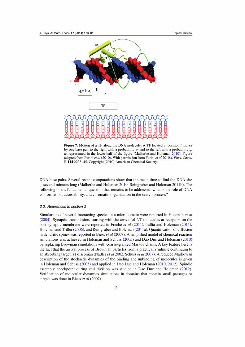
Figure 7. Motion of a TF along the DNA molecule. A TF located at position i movesby one base pair to the right with a probability pi and to the left with a probability qi
as represented in the lower half of the figure (Malherbe and Holcman 2010). Figureadapted from Furini et al (2010). With permission from Furini et al 2010 J. Phys. Chem.B 114 2238–45. Copyright (2010) American Chemical Society.
DNA base pairs. Several recent computations show that the mean time to find the DNA siteis several minutes long (Malherbe and Holcman 2010, Reingruber and Holcman 2011b). Thefollowing opens fundamental question that remains to be addressed: what is the role of DNAconformation, accessibility, and chromatin organization in the search process?
2.3. References to section 2
Simulations of several interacting species in a microdomain were reported in Holcman et al(2004). Synaptic transmission, starting with the arrival of NT molecules at receptors on thepost-synaptic membrane were reported in Freche et al (2011), Taflia and Holcman (2011),Holcman and Triller (2006), and Reingruber and Holcman (2011a). Quantification of diffusionin dendritic spines was reported in Biess et al (2007). A simplified model of chemical reactionsimulations was achieved in Holcman and Schuss (2005) and Dao Duc and Holcman (2010)by replacing Brownian simulations with coarse-grained Markov chains. A key feature here isthe fact that the arrival process of Brownian particles from a practically infinite continuum toan absorbing target is Poissonian (Nadler et al 2002, Schuss et al 2007). A reduced Markoviandescription of the stochastic dynamics of the binding and unbinding of molecules is givenin Holcman and Schuss (2005) and applied in Dao Duc and Holcman (2010, 2012). Spindleassembly checkpoint during cell division was studied in Dao Duc and Holcman (2012).Verification of molecular dynamics simulations in domains that contain small passages ortargets was done in Biess et al (2007).
15

J. Phys. A: Math. Theor. 47 (2014) 173001 Topical Review
Figure 8. Search scenario for a DNA target by a TF. The TF can attach to the DNAmolecule and scan a number of potential binding sites or diffuse freely in the nucleus.The TF alternates periods of one-dimensional random walks along the DNA moleculeand free diffusions in the nucleus.
3. Diffusion on a crowded membrane and intracellular trafficking
The organization of a cellular membrane is the determinant of the efficiency of traffickingmolecules (e.g., receptors) to their destination. After decades of intense research on membraneorganization, it was demonstrated recently by single-particle imaging that the effectivediffusion constant can span a large spectrum of values, from 0.001 to 0.2 μm2 s−1 (Choquet2010), yet it is still unclear how the heterogeneity of the membrane controls diffusion (seefigure 9). There are several studied examples, where changing the arrangement of absorbingwindows affects the cell function. In bacteria, receptors re-cluster, depending on the externalconcentration of a chemotactic attractant, thus improving the sensitivity. In the context ofneuroscience, receptors are known to re-cluster before the tip of a growing neuron (growthcone) turns toward a chemoattractant. Changing the arrangement of AMPA receptors inneuronal synapses affects the synaptic transmission. The variations in the shape of dendriticspines of neurons (Segal and Andersen 2000) as a result of learning and other physiologicalactivities changes both the density and distribution of receptors, transporters and otherregulatory proteins and thereby change the ionic flux through the membrane (Bourne andHarris 2008). Recently, using single molecule tracking, the diffusion coefficient of a moleculefreely diffusing on intact and treated neuronal membranes, cleared of almost all obstacles, wascalculated in (Renner et al 2009). The degree of crowding of a membrane with obstacles canbe estimated from diffusion data and from an appropriate model and its analysis, as explainedbelow. The key to assessing the crowding is to estimate the local diffusion coefficient fromthe measured molecular trajectories and from the analytical formula for the MFPT through anarrow passage between obstacles.
16

J. Phys. A: Math. Theor. 47 (2014) 173001 Topical Review
Figure 9. Organization of a neuronal membrane (www.nanobio.frontier.kyoto-u.ac.jp/lab/slides/4/e.html, reproduced with permission from A Kusumi,Copyright 2005) containing microdomains made of overlapping filaments.
3.1. Diffusion on a membrane crowded with obstacles
In a simplified model of crowding, the circular obstacles are as shown in figure 10(a). It is asquare lattice of circular obstacles of radius a centered at the corners of lattice squares of sideL. The mean exit time from a lattice box (see figure 10(a)) is to leading order
τ4 = τ
4, (3.1)
where τ is the MFPT to a single absorbing window in narrow straits with the other windowsclosed (reflecting instead of absorbing) (see figure 20 (left); τ is the MFPT from the head tothe segment AB, or figure 24 (left)). It follows that the waiting time in the cell enclosed by theobstacles is approximately exponentially distributed (1.1) with rate
λ = 2
τ4, (3.2)
17

J. Phys. A: Math. Theor. 47 (2014) 173001 Topical Review
(b)(a)
(d )(c)
Figure 10. Model of diffusion on a crowded membrane. (a) Schematic representation ofa Brownian particle diffusing in a crowded microdomain. (b) Mean square displacement(MSD) of the particle in a domain paved with microdomains. The MSD is linear, showingthat crowding does not affect the nature of diffusion. The effective diffusion coefficientis computed from 〈MSD(t)/4t〉. (c) Effective diffusion coefficient computed from theMSD for different radiuses of the obstacles. Brownian simulations (continuous curve):there are three regions (separated by the dashed lines). While there is no crowding fora < 0.2, the decreasing of the effective diffusion coefficient for 0.2 < a < 0.4 islogarithmic, and like square root for a > 0.4. (d) Effective diffusion coefficient of aparticle diffusing in a domain as a function of the fraction of the occupied surface. AnAMPAR has a diffusion coefficient of 0.2 μm2 s−1 in a free membrane.
where τ is given by
τ ≈
⎧⎪⎪⎪⎪⎨⎪⎪⎪⎪⎩
c1 for 0.8 < ε < 1,
c2|�| log1
ε+ d1 for 0.55 < ε < 0.8,
c3|�|√
ε+ d2 for ε < 0.55,
(3.3)
with ε = (L − 2a)/a and d1, d2 = O(1) for ε � 1 (see figure 10). The constantsci, (i = 1, 2, 3) are calculated in Holcman et al (2011): the MFPT c1 from the center to
18
J. Phys. A: Math. Theor. 47 (2014) 173001 Topical Review
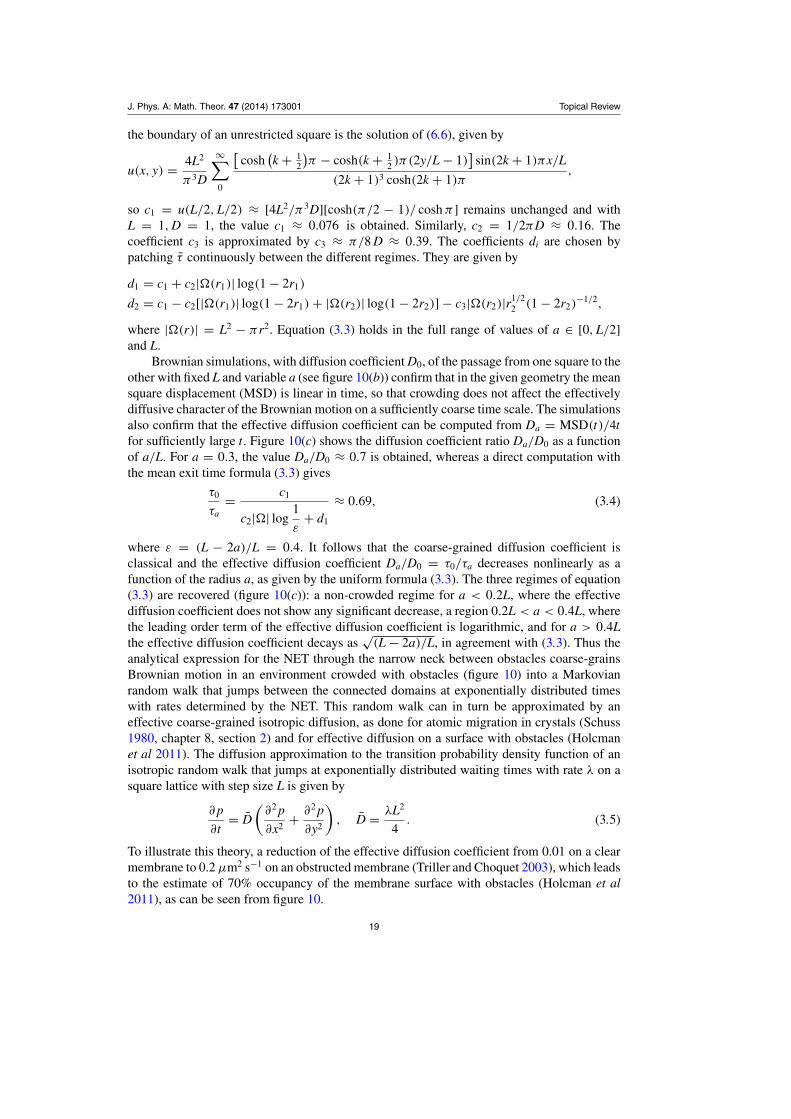
the boundary of an unrestricted square is the solution of (6.6), given by
u(x, y) = 4L2
π3D
∞∑0
[cosh
(k + 1
2
)π − cosh(k + 1
2 )π(2y/L − 1)]
sin(2k + 1)πx/L
(2k + 1)3 cosh(2k + 1)π,
so c1 = u(L/2, L/2) ≈ [4L2/π3D][cosh(π/2 − 1)/ cosh π ] remains unchanged and withL = 1, D = 1, the value c1 ≈ 0.076 is obtained. Similarly, c2 = 1/2πD ≈ 0.16. Thecoefficient c3 is approximated by c3 ≈ π/8 D ≈ 0.39. The coefficients di are chosen bypatching τ continuously between the different regimes. They are given by
d1 = c1 + c2|�(r1)| log(1 − 2r1)
d2 = c1 − c2[|�(r1)| log(1 − 2r1) + |�(r2)| log(1 − 2r2)] − c3|�(r2)|r1/22 (1 − 2r2)
−1/2,
where |�(r)| = L2 − πr2. Equation (3.3) holds in the full range of values of a ∈ [0, L/2]and L.
Brownian simulations, with diffusion coefficient D0, of the passage from one square to theother with fixed L and variable a (see figure 10(b)) confirm that in the given geometry the meansquare displacement (MSD) is linear in time, so that crowding does not affect the effectivelydiffusive character of the Brownian motion on a sufficiently coarse time scale. The simulationsalso confirm that the effective diffusion coefficient can be computed from Da = MSD(t)/4tfor sufficiently large t. Figure 10(c) shows the diffusion coefficient ratio Da/D0 as a functionof a/L. For a = 0.3, the value Da/D0 ≈ 0.7 is obtained, whereas a direct computation withthe mean exit time formula (3.3) gives
τ0
τa= c1
c2|�| log1
ε+ d1
≈ 0.69, (3.4)
where ε = (L − 2a)/L = 0.4. It follows that the coarse-grained diffusion coefficient isclassical and the effective diffusion coefficient Da/D0 = τ0/τa decreases nonlinearly as afunction of the radius a, as given by the uniform formula (3.3). The three regimes of equation(3.3) are recovered (figure 10(c)): a non-crowded regime for a < 0.2L, where the effectivediffusion coefficient does not show any significant decrease, a region 0.2L < a < 0.4L, wherethe leading order term of the effective diffusion coefficient is logarithmic, and for a > 0.4Lthe effective diffusion coefficient decays as
√(L − 2a)/L, in agreement with (3.3). Thus the
analytical expression for the NET through the narrow neck between obstacles coarse-grainsBrownian motion in an environment crowded with obstacles (figure 10) into a Markovianrandom walk that jumps between the connected domains at exponentially distributed timeswith rates determined by the NET. This random walk can in turn be approximated by aneffective coarse-grained isotropic diffusion, as done for atomic migration in crystals (Schuss1980, chapter 8, section 2) and for effective diffusion on a surface with obstacles (Holcmanet al 2011). The diffusion approximation to the transition probability density function of anisotropic random walk that jumps at exponentially distributed waiting times with rate λ on asquare lattice with step size L is given by
∂ p
∂t= D
(∂2 p
∂x2+ ∂2 p
∂y2
), D = λL2
4. (3.5)
To illustrate this theory, a reduction of the effective diffusion coefficient from 0.01 on a clearmembrane to 0.2 μm2 s−1 on an obstructed membrane (Triller and Choquet 2003), which leadsto the estimate of 70% occupancy of the membrane surface with obstacles (Holcman et al2011), as can be seen from figure 10.
19
J. Phys. A: Math. Theor. 47 (2014) 173001 Topical Review
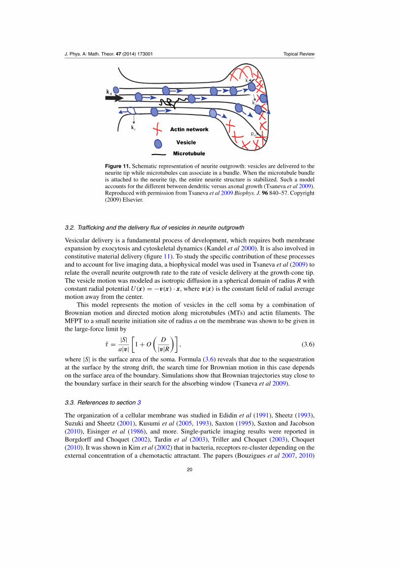
Figure 11. Schematic representation of neurite outgrowth: vesicles are delivered to theneurite tip while microtubules can associate in a bundle. When the microtubule bundleis attached to the neurite tip, the entire neurite structure is stabilized. Such a modelaccounts for the different between dendritic versus axonal growth (Tsaneva et al 2009).Reproduced with permission from Tsaneva et al 2009 Biophys. J. 96 840–57. Copyright(2009) Elsevier.
3.2. Trafficking and the delivery flux of vesicles in neurite outgrowth
Vesicular delivery is a fundamental process of development, which requires both membraneexpansion by exocytosis and cytoskeletal dynamics (Kandel et al 2000). It is also involved inconstitutive material delivery (figure 11). To study the specific contribution of these processesand to account for live imaging data, a biophysical model was used in Tsaneva et al (2009) torelate the overall neurite outgrowth rate to the rate of vesicle delivery at the growth-cone tip.The vesicle motion was modeled as isotropic diffusion in a spherical domain of radius R withconstant radial potential U (x) = −v(x) · x, where v(x) is the constant field of radial averagemotion away from the center.
This model represents the motion of vesicles in the cell soma by a combination ofBrownian motion and directed motion along microtubules (MTs) and actin filaments. TheMFPT to a small neurite initiation site of radius a on the membrane was shown to be given inthe large-force limit by
τ = |S|a|v|
[1 + O
(D
|v|R)]
, (3.6)
where |S| is the surface area of the soma. Formula (3.6) reveals that due to the sequestrationat the surface by the strong drift, the search time for Brownian motion in this case dependson the surface area of the boundary. Simulations show that Brownian trajectories stay close tothe boundary surface in their search for the absorbing window (Tsaneva et al 2009).
3.3. References to section 3
The organization of a cellular membrane was studied in Edidin et al (1991), Sheetz (1993),Suzuki and Sheetz (2001), Kusumi et al (2005, 1993), Saxton (1995), Saxton and Jacobson(2010), Eisinger et al (1986), and more. Single-particle imaging results were reported inBorgdorff and Choquet (2002), Tardin et al (2003), Triller and Choquet (2003), Choquet(2010). It was shown in Kim et al (2002) that in bacteria, receptors re-cluster depending on theexternal concentration of a chemotactic attractant. The papers (Bouzigues et al 2007, 2010)
20
J. Phys. A: Math. Theor. 47 (2014) 173001 Topical Review
show that receptors are known to re-cluster before the tip of a growing neuron. Taflia andHolcman (2011) and Freche et al (2011) show that rearrangement of AMPA receptors affectssynaptic transmission. Segal and Andersen (2000) report variations in the shape of dendriticspines of neurons as a result of learning and other physiological activities in changing boththe density and distribution of receptors, transporters, and other regulatory proteins. Changesin ionic flux through the membrane as the result of rearrangements are reported in Bourne andHarris (2008).
4. Physical virology: modeling the early steps of cell viral infection at themolecular level
The goal of this section is to present modeling for quantifying the early steps of cell viralinfection.
4.1. The cytoplasmic viral trafficking
Most viruses entering cells after binding to specific membrane receptors (Whittaker et al2000, Greber and Way 2006) are enveloped in an endosomal compartment (figure 12). Toundergo cytoplasmic or nuclear replication and to avoid degradation in acidic lysosomes,viruses must then successfully escape the endosome. Thus the Brownian motion of the viruscan be terminated by killing the trajectory (see section 4.2.1 below). Enveloped viruses, suchas influenza, contain membrane-associated glycoproteins, which mediate the fusion betweenthe viral and endosomal membranes. In particular, acidification of the endosome triggers theconformational change of the influenza hemagglutinins (HA) into a fusogenic state, leadingto endosome-virus membranes fusion and release of genes into the cytoplasm. Other non-enveloped viruses, such as the Adeno-Associated-Virus, have to escape the endosome, aprocess that requires one of the (less than 10) capsid proteins to change conformation.Following the endosomal escape, viruses have to travel through the crowded cytoplasm toreach the nucleus and deliver their genetic material through the nuclear pores. While thecytoplasmic movement of viral particles towards the nucleus is facilitated by the microtubularnetwork and viral proteins, very little is known about the fate of non-viral DNA vectors in thecytoplasm. However, trapping of large DNA particles (>500 kDa) in the crowded cytoplasmdrastically hinders their cytoplasmic diffusion (Verkman 2000, Dauty and Verkman 2005)and subsequently diminishes the transfection rate of synthetic gene vectors (see figure 13).Mathematical and physical models of this process are constructed for the purpose of predictingand quantifying infectivity and the success of gene delivery. The models give rise to rationalBrownian dynamics simulations for the study of sensitivity to parameters and, eventually,for testing the increase or the drop in infectivity by using simultaneously a combination ofvarious drugs. The modeling approach can be used for the optimization of the delivery in ahigh-dimensional parameter space.
For example, fusogenic peptides derived from viral glycoproteins, are increasingly usedin cationic synthetic vectors and the pH-sensitivity of fusogenic glycoproteins can now betuned by modifying the electrostatic stability of the fusogenic complex. These engineeredglycoproteins are intended for designing efficient gene vectors, so quantitative models can helpoptimizing glycoprotein molecular properties with respect to the endosomal escape efficacyof the vector.
4.2. Stochastic description of viral trajectories
Vesicular and viral motions alternate intermittently between periods of free diffusion anddirected motion along MTs. Such viral trajectories have been recently monitored by using
21

J. Phys. A: Math. Theor. 47 (2014) 173001 Topical Review
(a)
(b)
(c)
(d )
(e)
(f )
Figure 12. Common entry and uncoating mechanisms of selected nuclear-replicatingviruses. Viruses can undergo substantial uncoating in the cytoplasm before translocatinginto the nucleus; (a) HIV, (b) influenza virus. Alternatively, viruses can dock to theNPC and uncoat at the cytoplasmic side of the nuclear membrane; (c) adenovirus and(d) herpesvirus. They may possibly disassemble within the nuclear pore; (e) hepatitis Bvirus; (f) parvovirus Whittaker et al (2000). Reproduced with permission from Whittakeret al 2000 Annu. Rev. Cell Dev. Biol. 16 627–51. Copyright (2003) Annual Reviews.
new imaging techniques in vivo. The trajectory of a viral particle x(t) can be modeled as therandomly switching process
dx(t) ={√
2D dw for x(t) freeV dt for x(t) bound to a MT,
(4.1)
where w(t) is standard Brownian motion, D is the diffusion constant, and V (x) is the velocityfield of the directed motion along MTs.
The particle motion (4.1) can be coarse-grained by the stochastic equation
dx = b(x) dt +√
2D dw, (4.2)
22

J. Phys. A: Math. Theor. 47 (2014) 173001 Topical Review
Figure 13. Virus infection in cell. (a) Trajectories of single AAV-Cy5 particles: thetraces showing single diffusing virus particles were recorded at different times. Theydescribe various stages of AAV infection, e.g. diffusion in solution (1 and 2), touching atthe cell membrane (2), penetration of the cell membrane (3), diffusion in the cytoplasm(3 and 4), penetration of the nuclear envelope (4), and diffusion in the nucleoplasm(Seisenberger et al 2001). Reproduced with permission from Seisenberger et al 2001Science 294 1929–32. Copyright (2001) The American Association for the Advancementof Science. (b) Schematic description of early steps of infection for viral and syntheticvectors. Synthetic vectors are not assisted by active transport during their cytoplasmictrafficking.
where b(x) is a drift that accounts for ballistic periods along MTs. The stochastic dynamics(4.2) can be used to generate computer simulations of trajectories in free and confinedenvironment (Schuss 2010b). It can also be used to derive asymptotic formulas for theprobability and the MFPT of the virus to a nuclear pore (Holcman 2007). Various analyticexpressions for the effective drift have been derived for various geometries. The expressionfor b(x) depends on the MT organization and on the viral dynamical properties, such as thediffusion constant D, affinity with MTs, and net velocity along MTs.
4.2.1. NET with killing. Consider the diffusion process x(t) defined by the stochasticdynamics in a domain �
dx = a(x) dt +√
2B(x) dw(t), (4.3)
where a(x) is a smooth drift vector, B(x) is a diffusion tensor, and w(t) is a vector ofindependent standard Brownian motions. If the trajectories x(t) can be terminated at time tat each point x ∈ � with probability k(x, t)t + o(t), the function k(x, t) is called killingmeasure (Schuss 2010b). When the boundary ∂� admits no absorption flux, except for a smallabsorbing window ∂�a, the NET problem is to find the absorption flux of trajectories thatsurvive the killing. Thus there are two random termination times defined on the trajectoriesx(t), the time T to termination by killing and the time τ to termination by absorption in ∂�a.
4.2.2. The probability of absorbed trajectories. The transition probability density function ofthe process x(t) with killing and absorption is the conditional transition probability density
23

J. Phys. A: Math. Theor. 47 (2014) 173001 Topical Review
function of trajectories that have neither been killed nor absorbed in ∂�a by time t,
p(x, t | y) dx = Pr{x(t) ∈ x + dx, T > t, τ > t | y}. (4.4)
It is the solution of the Fokker–Planck equation (Schuss 2010b)∂ p(x, t | y)
∂t= Lx p(x, t | y) − k(x)p(x, t | y) for x, y ∈ �, (4.5)
where Lx is the forward operator
Lx p(x, t | y) =d∑
i, j=1
∂2σ i, j(x)p(x, t | y)
∂xi∂x j−
d∑i=1
∂ai(x)p(x, t | y)
∂xi, (4.6)
and σ(x) = 12 B(x)BT (x). The operatorLx can be written in the divergence formLx p(x, t | y) =
−∇ · J(x, t | y), where the flux density vector J(x, t | y) is
Ji(x, t | y) = −d∑
j=1
∂σ i, j(x)p(x, t | y)
∂xi+ ai(x)p(x, t | y). (4.7)
The initial and boundary conditions for the Fokker–Planck equation (4.5) are
p(x, 0 | y) = δ(x − y) for x, y ∈ � (4.8)
p(x, t | y) = 0 for t > 0, x ∈ ∂�a, y ∈ � (4.9)
J(x, t | y) · n(x) = 0 for t > 0, x ∈ ∂� − ∂�a, y ∈ �. (4.10)
The probability that the particle reaches the absorbing ∂�a before being killed is given byHolcman et al (2005b) and Schuss (2010b)
Pr{T < τ | y} =∫ ∞
0
∫�
k(x)p(x, t | y) dx dt. (4.11)
The absorption probability flux on ∂�A is J(t | y) = ∮∂�
J(x, t | y) ·n(x) dSx and∫ ∞
0 J(t | y) dtis the probability of trajectories that have ever been absorbed at ∂�a.
The probability distribution function of the killing time T is the conditional probabilityof killing before time t of trajectories that have not been absorbed in ∂�a by that time,
Pr{T < t | τ > t, y} = Pr{T < t, τ > t | y}Pr{τ > t | y} =
∫ t0
∫�
k(x)p(x, s | y) dx ds∫ ∞0
∫�
k(x)p(x, s | y) dx ds.
The probability distribution of the time to absorption at ∂�a is the conditional probability ofabsorption before time t of trajectories that have not been killed by that time,
Pr{T < t | τ > t, y} =∫ t
0 J(s | y) ds
1 − ∫ ∞0
∫�
k(x)p(x, s | y) dx ds. (4.12)
Thus the NET is the conditional expectation of the absorption time of trajectories that are notkilled in �, that is,
E[τ | T > τ, y] =∫ ∞
0Pr{τ > t | T > τ, y} dt =
∫ ∞0 sJ(s | y) ds
1 − ∫ ∞0
∫�
k(x)p(x, s | y) dx ds.
The survival probability of trajectories that have not been terminated by time t is given by
S(t | y) =∫
�
p(x, t | y) dx. (4.13)
The mean time spent at x prior to termination,
p(x | y) =∫ ∞
0p(x, t | y) dt (4.14)
24

J. Phys. A: Math. Theor. 47 (2014) 173001 Topical Review
is the solution of the boundary value problem
Lx p(x | y) − k(x) p(x | y) = −δ(x − y) for x, y ∈ �
p(x | y) = 0 for x ∈ ∂�a, y ∈ � (4.15)
J(x | y) · n(x) = 0 for t > 0, x ∈ ∂� − ∂�a, y ∈ �.
If the initial pdf is a sufficiently smooth function pI (x), the density of the time spent at x priorto termination,
p(x) =∫
�
p(x | y)pI(y) dy, (4.16)
satisfies
Lx p(x) − k(x) p(x) = −pI (x) for x ∈ � (4.17)
p(x) = 0 for x ∈ ∂�a
J(x) · n(x) = 0 for t > 0, x ∈ ∂� − ∂�a.
The probability PN of trajectories that start at y ∈ � and are terminated at ∂�a is
PN =∫
�
Pr{τ 〈T | x(0) = y}pI(y) dy = 1 −∫
�
k(x) p(x) dx. (4.18)
4.3. Probability that a viral particle arrives alive at a nuclear pore
For Brownian motion with diffusion coefficient 1 (without drift) the boundary value problem(4.17) can be solved asymptotically for a small absorbing window ∂�a in terms of the Neumannfunction N(x, ξ), which is a solution of the boundary value problem
xN(x, ξ) = −δ(x − ξ) for x, ξ ∈ �,
∂N(x, ξ)
∂n(x)= − 1
|∂�| for x ∈ ∂�, ξ ∈ �, (4.19)
and is defined up to an additive constant. Multiplying (4.17) by N(x, ξ) and using Green’stheorem, the identity
p(ξ) = −∫
�
N(x, ξ)[−pI (x) + k(x) p(x)]dx +∫
∂�a
N(x, ξ)∂ p(x)
∂ndSx + 1
|∂�|∫
∂�
p(x) dSx
is obtained. The leading order term in the expansion of p(x) for small |∂�a| and sufficientlysmall killing rate k(x, t) (i.e., smaller than the absorption rate, see Holcman (2007)) is constantp(x) ≈ Pa outside a boundary layer near ∂�a. Then the following approximation is valid,
p(ξ) ≈∫
∂�a
N(x, ξ)∂ p(x)
∂ndSx + Pa
(1 −
∫�
k(x)N(x, ξ) dx)
+∫
�
N(x, ξ)pI (x) dx.
The compatibility condition, obtained from the integration of (4.17) over �, and the boundarylayer expansion (see Holcman (2007)), give in the three-dimensional case the approximationof the density of the time spent at x ∈ � as
Pa ≈ 1
4ε + ∫�
k(x) dx, (4.20)
provided (see Schuss 2013 and Holcman and Schuss 2014)
|∂�|1/(d−1)
|�|1/d= O(1) for ε � 1, (4.21)
25

J. Phys. A: Math. Theor. 47 (2014) 173001 Topical Review
and the probability of the absorbed trajectories as
PN = 1 −∫
�
k(x) p(x) dx ≈ 4ε
4ε + ∫�
k(x) dxfor k(x) � 1. (4.22)
If the diffusion coefficient is D, the parameter ε in (4.20) and (4.22) is changed to Dε. Thecase of Brownian motion with drift is described in Holcman (2007). The results of this sectionare used to estimate the probability that a live virus arrives at one of the small pores in a cell’snucleus.
4.4. The mean arrival time to a small nuclear pore
The crowded cytoplasm is a risky environment for gene vectors that can be either trapped ordegraded through the cellular defense machinery. Thus cytoplasmic trafficking is rate-limitingand to analyze quantitatively that step, asymptotic expressions for the probability PN and themean arrival time Eτ of a virus vector to one of n small nuclear pores ∂�a were derived inHolcman (2007) and Lagache et al (2009b).
Viral degradation or immobilization is modeled as a steady state degradation rate k(x).The probability density function p(x, t) of viral trajectories that survive by time t in thecytoplasm � is defined as the joint probability and density of the trajectory, the killing timeT , and the time to absorption τ ,
p(x, t) dx = Pr{x(t) ∈ x + dx, T > t, τ > t} (4.23)
with initial viral pdf pI(x). The probability PN of trajectories that start with the viral pdf in� and are terminated at ∂�a is calculated from the expression for the NET as follows. For nidentical nuclear pores in the shape of absorbing disks of radius ε and when b(x) = −∇ (x)
for some potential (x), the leading order terms in the expansions of PN and Eτ for small ε
are given by Amoruso et al (2011) as
PN ≈1
|∂�|∮∂�
exp{ − (x)
D
}dx
1|∂D|
∮∂D exp
{ − (x)
D
}dx + (
14nDε
+ 1DC�
) ∫�
k(x) exp{ − (x)
D
}dx
and
Eτ ≈(
14nDε
+ 1DC�
) ∫�
exp{ − (x)
Dcal
}dx
1|∂D|
∮∂D exp
{ − (x)
D
}dx + (
14nDε
+ 1DC�
) ∫�
k(x) exp{ − (x)
D
}dx
,
where C� is the capacity of the nucleus (for a sphere of radius δ, C� = 4πδ). Interestingly, fora biological cell with a spherical nucleus (radius δ = 5 μm ), the n = 2000 circular nuclearpores (radius ε = 25 nm ) cover a surface nπε2/4πδ2 ≈ 1% of the total nuclear surface and1/4nDε is only one third of 1/C�.
4.5. Endosomal viral escape
Once a virus enters an endosome, it has to escape into the cytoplasm before being degraded bylysosomes. Although the exact pathways leading to endosomal escape are not fully elucidated,they are limiting steps. Most viruses possess efficient endosomolytic proteins allowing themto disrupt the endosomal membrane, such as the VP1 penetration protein of the adeno-associated virus or the influenza HA. In addition, the biophysical mechanism leading toendosomal membrane destabilization and concomitant plasmids release for synthetic vectorsis still poorly understood. However, in both cases, acidification of the endosome is neededto trigger endosomal escape. For viruses, protons or low pH-activated proteases bind viralendosomolytic proteins, triggering their conformational change into a fusogenic state. The
26

J. Phys. A: Math. Theor. 47 (2014) 173001 Topical Review
case of proton-binding sites on the viral envelope of the influenza virus has also been discussed(see references below).
Models aimed at estimating the residence time of a viral particle inside an endosomalcompartment are based on the assessment of the accumulation of discrete proton-bindingevents, that lead to the conformational change of HAs. These models, for both envelopedand non-enveloped viruses, consist of two steps. In the first step, the concentration of protonsis fixed and the mean time for protons to bind to fundamental protein binding sites until athreshold is reached is calculated from a jump-Markov-process model by asymptotic methods.A conformational change into a fusogenic state is triggered after the threshold is reached. Inthe second step, the dynamics of endosomal escape is modeled by coupling the pH-dependentconformational change of glycoproteins with the proton-influx rate. The impact of the size ofthe endosome on the escape kinetics and pH can be mathematically predicted. It reconcilesdifferent experimental observations: while a virus can escape from small endosomes (radiusof 80 nm) in the cell periphery at pH ∼ 6 in about 10 min, it can also be routed towards thenuclear periphery, where escape from larger endosomes (radius of 400 nm) is rapid (less than1 min) at pH = 5. The detailed modeling of these two steps were reviewed in Amoruso et al(2011).
4.6. References to section 4
Mathematical and physical models of the viral infection process were proposed in Holcman(2007), Lagache and Holcman (2008a, 2008b), Amoruso et al (2011), Lagache et al (2009a).Optimization of the virus delivery in a high-dimensional parameter space is discussed inLagache et al (2012). Synthetic vectors are discussed in Abe et al (1998) and Tu and Kim(2008). Tuning of the pH-sensitivity of fusogenic glycoproteins is discussed in Rachakondaet al (2007). Escape efficacy of the vector is discussed in Sodeik (2000).
Vesicular and viral motions that alternate intermittently between periods of free diffusionand directed motion along MTs are discussed in Greber and Way (2006). Such viral trajectorieshave been recently monitored by using new imaging techniques in vivo (Seisenberger et al2001, Brandenburg and Zhuang 2007).
The MFPT of a virus to a nuclear pore was calculated in Holcman (2007). The effectivedrifts of viral motion have been derived for various geometries in Lagache and Holcman(2008a, 2008b).
The adeno-associated virus and the influenza HA have been discussed in Farr et al (2005)and Huang et al (2002). Models aimed at estimating the residence time of a viral particle insidean endosomal compartment are considered in Lagache et al (2012). The key to the calculationof the MFPT of the Markovian jump process model is the method of Knessl et al (1984a),Matkowsky et al (1984) and Knessl et al (1984b). The detailed modeling of two key steps inthe viral release was reviewed in Amoruso et al (2011).
5. The NET in neurobiology and synaptic transmission
As mentioned above, the NET reflects the role of the cell’s geometrical structure in determiningthe cell’s biological function. Next, illustrations are given of the way the NET is manifestedin modeling synaptic transmission and in the simulation, analysis, and interpretation of theoutput of the models. The explicit asymptotic formulas for the NET also coarse-grain spatialorganization of a fundamental domain, called the PSD, which is discussed in detail below.
To address the structure-function question in molecular-level cell models, the discussion isfocused on the regulation of diffusion flux in synapses and dendritic spines of neurons, whose
27

J. Phys. A: Math. Theor. 47 (2014) 173001 Topical Review
Figure 14. A neuronal synapse. Left panel: electron microscopy of a synapse. Thepost-synaptic terminal is located on a dendritic spine (S) branched in the dendrite (D).The glial cells (G) are located around the axon (A). (Spacek J 2002). Reproduced withpermission from Spacek J 2002 Psychiatrie, Suppl. 3 6 55–60. Copyright (2002) Tigis.Right panel: schematic representation of a synapse between neurons. Neurotransmitters(blue) are released to the synaptic cleft at the presynaptic terminal and can find a receptor(green) on the post-synaptic terminal or be absorbed by the surrounding glial cells (red).The post-synaptic density (PSD) is the dense region above the yellow sheet holding thescaffolding molecules (orange).
spatial structure has been studied extensively (see list of references below). A schematicrepresentation of a synapse between neurons is given in figure 14.3 By its very definition,synapses are local active micro-contacts underlying direct neuronal communication butdepending on the brain area where they are located and their specificity, they can vary insize and molecular composition. The molecular processes underlying synaptic transmissionare well known: after NTs such as glutamate, released from a vesicle located on the surfaceof a pre-synaptic neuron (see figure 14), they diffuse inside the synaptic cleft, composed ofpre- and post-synaptic terminals. The post-synaptic terminal of an excitatory synapse containsionotropic glutamate receptors such as AMPA and NMDA and they may open upon bindingto NTs. When NTs diffuse in the cleft, they can either find a specific receptor protein on themembrane of the post-synaptic terminal, such as NMDA, AMPA, and so on4, or are absorbedby the surrounding glia cells and recycled. Relevant terminology, illustrations, and movies forthe biological material can be found in Wikipedia. More generally, there are various types ofsynapses characterized by the NT molecules, such as the small molecules acetylcholine (ACh),dopamine (DA), norepinephrine (NE), serotonin (5-HT), histamine, epinephrine, or the aminoacids gamma-aminobutyric acid (GABA), glycine, glutamate, aspartate, and many others5 thatare released at the presynaptic terminal into the flat cylindrically-shaped synaptic cleft whenan action potential (signal) reaches the presynaptic terminal. Once a receptor binds a ligandNT molecule (or molecules) it opens to the passage of ions, which diffuse in the cleft fromthe pre- to the post-synaptic terminal (also called neuronal spine), thus transmitting the signal
3 This lower figure is based on www.niaaa.nih.gov/Resources/GraphicsGallery/Neuroscience/Pages/synapsebetween_neurons.aspx.4 see, e.g. http://en.wikipedia.org/wiki/Biochemical_receptor.5 see, e.g., http://en.wikipedia.org/wiki/Neurotransmitter.
28
J. Phys. A: Math. Theor. 47 (2014) 173001 Topical Review
across the synapse into the neuronal spine. The signal propagates in the form of a diffusionflux of ions, such as calcium or sodium, through the spine neck into the dendrite (see idealizedmathematical models of spine structure in figure 20).
For example, AMPA receptors are tetrameric assemblies composed of four differentsubunits, which can bind to a glutamate molecule. However, two glutamate molecules arerequired to open a single AMPA channel. The amplitude of ionic current is thus proportionalto the number of open receptors and their conductances. The post-synaptic current measuresthe efficiency of synaptic transmission and is related to the frequency and location of releasedvesicles in a complex manner (see list of references below).
This section reviews some properties of synaptic transmission based on a diffusion modelin microdomains. The presented methods serve to estimate the mean and the variance of thepost-synaptic current. Indeed, this current plays a fundamental role in neuronal communication:it is the direct and fast signal of synaptic transmission. It activates the post-synaptic neuron ormodulates its membrane potential. This current not only depends on receptors such as AMPA,but also on the complex molecular machinery edifice underneath that controls them. Possiblechanges in the current dynamics is the readout of synaptic plasticity, a process that underlieslearning and memory.
The transmitted diffusion flux can be regulated by the number and distribution of thereceptors, by the length of the spine neck, the number and distribution of ionic channels andpumps on the spine neck that can leak ions from the neck, and many other structural factors.Mathematical models of synapse components provide much information about their function(see section 5.3 below).
5.1. A model of the synaptic current
A general approach to the estimation of the synaptic current is proposed next. The diffusionof glutamate molecules in the cleft geometry, which is approximated by a flat cylinder, isdescribed by a direct analysis of AMPA conductances rather than by the classical Markovdescription, obtained by optimal fitting of measurements performed outside a synapse. Thepresented method accounts for the four glutamate binding sites per receptor. While glutamatemolecules are Brownian inside the cylindrical synaptic cleft �, AMPARs are positioned onthe PSD (see figures 14 (right) and 16 (right)). The model of glutamate binding to an AMPARis a radiative boundary condition on the PSD (�PSD), as described below.
When a glutamate molecule hits the lateral boundary (∂�Lat) of the cleft (modeled as acylinder �), it is absorbed and no longer can contribute to the activation of AMPARs. The pdfp(x, t|x0) of a Brownian glutamate molecule x(t), given x(0) = x0 ∈ �, is the solution of theinitial-boundary value problem for the diffusion equation
∂ p(x, t|x0)
∂t= Dp(x, t|x0) for x ∈ �, t > 0 (5.1)
p(x, 0) = δ(x − x0) for x ∈ �
∂ p(x, t|x0)
∂ν= 0 for x ∈ ∂�r
p(x, t|x0) = 0 for x ∈ ∂�Lat
−D∂ p(x, t|x0)
∂ν= −κ p(x, t|x0) for x ∈ ∂�PSD, (5.2)
where D is diffusion constant of a free glutamate molecule. The partial absorption rate constantκ not only accounts for the fraction of AMPARs inside the PSD, but also for the activation
29
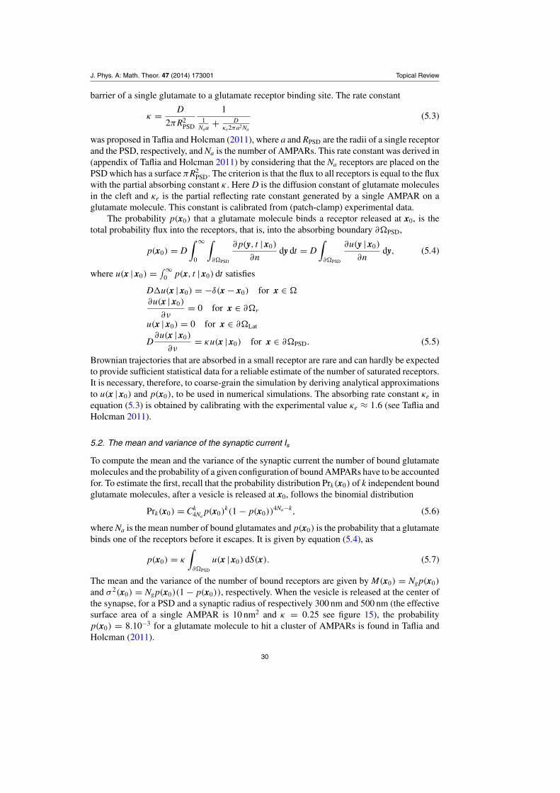
J. Phys. A: Math. Theor. 47 (2014) 173001 Topical Review
barrier of a single glutamate to a glutamate receptor binding site. The rate constant
κ = D
2πR2PSD
11
Naa + Dκe2πa2Na
(5.3)
was proposed in Taflia and Holcman (2011), where a and RPSD are the radii of a single receptorand the PSD, respectively, and Na is the number of AMPARs. This rate constant was derived in(appendix of Taflia and Holcman 2011) by considering that the Na receptors are placed on thePSD which has a surface πR2
PSD. The criterion is that the flux to all receptors is equal to the fluxwith the partial absorbing constant κ . Here D is the diffusion constant of glutamate moleculesin the cleft and κe is the partial reflecting rate constant generated by a single AMPAR on aglutamate molecule. This constant is calibrated from (patch-clamp) experimental data.
The probability p(x0) that a glutamate molecule binds a receptor released at x0, is thetotal probability flux into the receptors, that is, into the absorbing boundary ∂�PSD,
p(x0) = D∫ ∞
0
∫∂�PSD
∂ p(y, t | x0)
∂ndy dt = D
∫∂�PSD
∂u(y | x0)
∂ndy, (5.4)
where u(x | x0) = ∫ ∞0 p(x, t | x0) dt satisfies
Du(x | x0) = −δ(x − x0) for x ∈ �
∂u(x | x0)
∂ν= 0 for x ∈ ∂�r
u(x | x0) = 0 for x ∈ ∂�Lat
D∂u(x | x0)
∂ν= κu(x | x0) for x ∈ ∂�PSD. (5.5)
Brownian trajectories that are absorbed in a small receptor are rare and can hardly be expectedto provide sufficient statistical data for a reliable estimate of the number of saturated receptors.It is necessary, therefore, to coarse-grain the simulation by deriving analytical approximationsto u(x | x0) and p(x0), to be used in numerical simulations. The absorbing rate constant κe inequation (5.3) is obtained by calibrating with the experimental value κe ≈ 1.6 (see Taflia andHolcman 2011).
5.2. The mean and variance of the synaptic current Is
To compute the mean and the variance of the synaptic current the number of bound glutamatemolecules and the probability of a given configuration of bound AMPARs have to be accountedfor. To estimate the first, recall that the probability distribution Prk(x0) of k independent boundglutamate molecules, after a vesicle is released at x0, follows the binomial distribution
Prk(x0) = Ck4Na
p(x0)k(1 − p(x0))
4Na−k, (5.6)
where Na is the mean number of bound glutamates and p(x0) is the probability that a glutamatebinds one of the receptors before it escapes. It is given by equation (5.4), as
p(x0) = κ
∫∂�PSD
u(x | x0) dS(x). (5.7)
The mean and the variance of the number of bound receptors are given by M(x0) = Ngp(x0)
and σ 2(x0) = Ngp(x0)(1 − p(x0)), respectively. When the vesicle is released at the center ofthe synapse, for a PSD and a synaptic radius of respectively 300 nm and 500 nm (the effectivesurface area of a single AMPAR is 10 nm2 and κ = 0.25 see figure 15), the probabilityp(x0) = 8.10−3 for a glutamate molecule to hit a cluster of AMPARs is found in Taflia andHolcman (2011).
30

J. Phys. A: Math. Theor. 47 (2014) 173001 Topical Review
0 0.05 0.1 0.15 0.2 0.25 0.3 0.35 0.4 0.45 0.5
0.2
0.25
0.3
0.35
0.4
0.45
0.5
PSD radius (µm)
CV
(A)
0 2000 4000 6000 8000 10000 120000
50
100
150
200
250
300
Glutamate moleclules
Cur
rent
(pA
)
(B)
ka=1.6
ka=1.5
ka=1.4
Figure 15. (A) The coefficient of variation (CV) reaches a maximum for a PSD ofradius of 0.3 μm. This shows that for a given size of the active zone, where vesicles arereleased, the CV is minimum when receptors are spread over an optimal PSD area. (B)Calibration of the partial absorption rate constant κ . The synaptic current is simulatedaccording to (5.9) for different values of the activation coefficient κ (see (5.3)). Theoptimal synaptic response in the range of 3000–12000 glutamate molecules is achievedat κ = 1.6.
An additional source of fluctuations in the number of bound AMPARs is as follows.AMPARs can bind from zero to four glutamate molecules. Therefore the probability Pr{�n | k}of a given configuration �n = (n4, n3, n2, n1) of n1 AMPARs that bind one glutamate molecule,n2 AMPARs that bind 2, and so on, when there are Na AMPA receptors and k < 4Na boundglutamate molecules, is given by
Pr{�n | k} = Na!
n4!n3!n2!n1!(Na − (n4 + n3 + n2 + n1))!
1
F(k, Na). (5.8)
This is the probability of choosing at random n4 AMPARs out of N4, n3 out of Na − n4, andso on. F(k, Na) is the total number of possibilities to decompose the number k as a sum ofNa summands from the set of integers {4, 3, 2, 1, 0}. The number F(k, Na) can be computednumerically as the (k + 1)th coefficient in the expansion of (1 + x + x2 + x3 + x4)Na in powersof x. With the notation V for the potential and �γ = (γ1, γ2, γ3, γ4) for the conductance vector,given these probabilities, all moments of the current can be found, and in particular, the meanand variance are given by
〈Is(x0)〉 =Ng∑
k=1
∑n∈Sk
�n · �γ Pr{�n | k}V Prk(x0)
=4Na∑k=1
∑n∈Sk
�n · �γ Pr{�n | k}Prk(x0)V + Naγ4V
(1 −
4Na∑k=0
Prk(x0)
)
〈I2s (x0)〉 =
Ng∑k=1
∑n∈Sk
(�n · �γ )2 Pr{�n | k}Prk(x0)V2 − 〈Is(x0)〉2
4Na∑k=1
∑n∈Sk
(�n · �γV )2 Pr{�n | k}Prk(x0)
+ (Naγ4V )2
(1 −
4Na∑k=0
Prk(x0)
)− 〈Is(x0)〉2. (5.9)
31

J. Phys. A: Math. Theor. 47 (2014) 173001 Topical Review
Here Sk is the set of all the possible configurations of �n = (n1, n2, n3, n4) such that4n4 + 3n3 + 2n2 + n1 = k. The formulae for the mean and variance are composed of twoterms: in the first one, the summation extends over sites that do not bind the maximal numberof glutamate molecules. The probability for such an event is the product of the probabilitiesPrk, that k glutamates are bound (k < 4Na) and the probability Pr{�n | k} for a given bindingconfiguration k = 4n4 + 3n3 + 2n2 + n1. The second term accounts for the event where allAMPAR binding sites are occupied (4Na), the probability is the complementary to the oneassociated with the partial binding of the first case. Figure 15(A) shows that the coefficientof variation (CV = SD/Mean, where SD stands for standard deviation) has a minimum asa function of the size of the PSD. This unexpected result is further discussed in Taflia andHolcman (2011).
5.3. Leakage in a conductor of Brownian particles
A conductor of Brownian particles is a bounded domain �, with a source of particles on theboundary or in the interior and a target, which is an absorbing part ∂�a of ∂�. The remainingboundary ∂�r is reflecting. Some of the Brownian particles may leak out of � not through∂�a if ∂�r contains a small absorbing hole S(ε). The calculation of the leakage flux is not thesame as that in the narrow escape problem, because the boundary flux does not vanish as thesmall hole shrinks. The leakage problem is to find the flux through the small hole S(ε).
The (dimensionless) stationary density u(x) of the Brownian particles satisfies the mixedboundary value problem
Du(x) = 0 for x ∈ �
∂u(x)
∂ν= 0 for x ∈ ∂�r
−D∂u(x)
∂ν= φ(x) for x ∈ ∂�s
u(x) = 0 for x ∈ ∂�a ∪ S(ε). (5.10)
The leakage flux,
Jε = D∫
S(ε)
∂u(x)
∂νdSx, (5.11)
is given in terms of the solution u0(x) of the reduced problem (without the leak S(ε)). Theleakage flux Jε can be found by determining the flux of each eigenfunction and then by usingeigenfunction expansion. The eigenvalue problem for (5.10) is
− Duε(x) = λ(ε)uε(x) for x ∈ � (5.12)
∂uε(x)
∂ν= 0 for x ∈ ∂�s ∪ ∂�r (5.13)
uε(x) = 0 for x ∈ S(ε) ∪ ∂�a. (5.14)
The eigenvalues have a regular expansion
λ(ε) = λ(0) + λ1ε + o(ε), (5.15)
where λ(0) is the eigenvalue of the reduced problem. The reduced Green function is thesolution of the mixed boundary value problem with D = 1,
− G(x, y) = δ(x − y) for x, y ∈ � (5.16)
∂G(x, y)
∂ν= 0 for x ∈ ∂�s ∪ �r, y ∈ � (5.17)
32

J. Phys. A: Math. Theor. 47 (2014) 173001 Topical Review
G(x, y) = 0, for x ∈ ∂�a, y ∈ �. (5.18)
Multiplying (5.16) by uε(x) and integrating over �, we get
uε(x) = −λ(ε)
∫�
G(x, y)uε(y) dy +∫
S(ε)
G(x, y)∂uε(y)
∂νdSy. (5.19)
In view of the boundary condition (5.14), equation (5.19) gives for all x ∈ S(ε)
λ(ε)
∫�
G(x, y)uε(y) dy =∫
S(ε)
G(x, y)∂uε(y)
∂νdSy. (5.20)
The integral on the left hand side of (5.20) can be expanded about the center of S(ε) in theform ∫
�
λ(ε)G(x, y)uε(y) dy = G0(ε) + O(|x|) for x ∈ S(ε), (5.21)
where the origin is assumed to be at the center of S(ε) and the (x1, x2) plane is that of S(ε).Using Popov’s theorem (Popov 1992, Schuss 2013, Holcman and Schuss 2014), the followingtwo equations are obtained (Singer et al 2008)
λ(ε)
∫�
uε(x) dx = 4εDG0(ε) + O(ε2 log ε)
1 + O(ε log ε)+ O(ε2 log ε) + D
∫∂�a
∂uε(y)
∂νdSy
G0(ε) = λ(ε)
∫�
G(0, y)uε(y) dy. (5.22)
This gives
λ(ε)
∫�
uε(x) dx = 4εDλ(ε)
∫�
G(0, y)uε(y) dy + O(ε2 log ε)
1 + O(ε log ε)
+ O(ε2 log ε) + D∫
∂�a
∂uε(y)
∂νdSy.
Solving for λ(ε) gives
λ(ε) = D∫∂�a
∂uε (y)
∂νdSy + O(ε2 log ε)∫
�uε(x) dx − 4εD
1+O(ε log ε)
∫�
G(0, y)uε(y) dy + O(ε2 log ε)
= D∫∂�a
∂uε (y)
∂νdSy∫
�uε(x) dx
(1 + 4εD
∫�
G(0, y)uε(y) dy∫�
uε(x) dx
)+ O(ε2 log ε). (5.23)
Note that due to (5.15),
D∫∂�a
∂uε (y)
∂νdSy∫
�uε(x) dx
= λ(0) + O(ε). (5.24)
Obviously, uε → u0 as ε → 0, where u0 is the corresponding eigenfunction of the reducedproblem (see also Ward and Keller 1993), so
limε→0
∫�
G(x, y)uε(y) dy =∫
�
G(x, y)u0(y) dy
limε→0
∫∂�a
∂uε(y)
∂νdSy =
∫∂�a
∂u0(y)
∂νdSy.
Therefore (5.22) gives the flux of uε(x) through the small hole as
J(ε) = D∫
S(ε)
∂uε(y)
∂νdSy = 4ελ(0)D
∫�
G(0, y)u0(y) dy + O(ε2 log ε)
= 4εDu0(0) + O(ε2 log ε). (5.25)
33
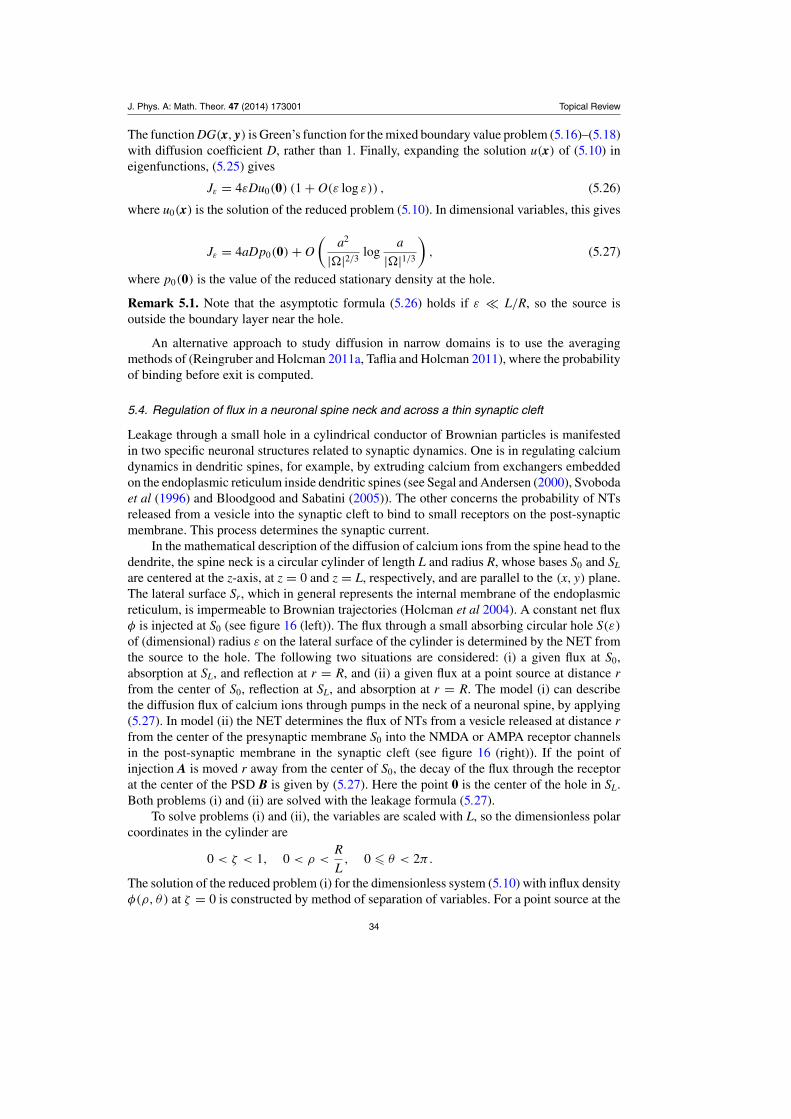
J. Phys. A: Math. Theor. 47 (2014) 173001 Topical Review
The function DG(x, y) is Green’s function for the mixed boundary value problem (5.16)–(5.18)with diffusion coefficient D, rather than 1. Finally, expanding the solution u(x) of (5.10) ineigenfunctions, (5.25) gives
Jε = 4εDu0(0) (1 + O(ε log ε)) , (5.26)
where u0(x) is the solution of the reduced problem (5.10). In dimensional variables, this gives
Jε = 4aDp0(0) + O
(a2
|�|2/3log
a
|�|1/3
), (5.27)
where p0(0) is the value of the reduced stationary density at the hole.
Remark 5.1. Note that the asymptotic formula (5.26) holds if ε � L/R, so the source isoutside the boundary layer near the hole.
An alternative approach to study diffusion in narrow domains is to use the averagingmethods of (Reingruber and Holcman 2011a, Taflia and Holcman 2011), where the probabilityof binding before exit is computed.
5.4. Regulation of flux in a neuronal spine neck and across a thin synaptic cleft
Leakage through a small hole in a cylindrical conductor of Brownian particles is manifestedin two specific neuronal structures related to synaptic dynamics. One is in regulating calciumdynamics in dendritic spines, for example, by extruding calcium from exchangers embeddedon the endoplasmic reticulum inside dendritic spines (see Segal and Andersen (2000), Svobodaet al (1996) and Bloodgood and Sabatini (2005)). The other concerns the probability of NTsreleased from a vesicle into the synaptic cleft to bind to small receptors on the post-synapticmembrane. This process determines the synaptic current.
In the mathematical description of the diffusion of calcium ions from the spine head to thedendrite, the spine neck is a circular cylinder of length L and radius R, whose bases S0 and SL
are centered at the z-axis, at z = 0 and z = L, respectively, and are parallel to the (x, y) plane.The lateral surface Sr, which in general represents the internal membrane of the endoplasmicreticulum, is impermeable to Brownian trajectories (Holcman et al 2004). A constant net fluxφ is injected at S0 (see figure 16 (left)). The flux through a small absorbing circular hole S(ε)
of (dimensional) radius ε on the lateral surface of the cylinder is determined by the NET fromthe source to the hole. The following two situations are considered: (i) a given flux at S0,absorption at SL, and reflection at r = R, and (ii) a given flux at a point source at distance rfrom the center of S0, reflection at SL, and absorption at r = R. The model (i) can describethe diffusion flux of calcium ions through pumps in the neck of a neuronal spine, by applying(5.27). In model (ii) the NET determines the flux of NTs from a vesicle released at distance rfrom the center of the presynaptic membrane S0 into the NMDA or AMPA receptor channelsin the post-synaptic membrane in the synaptic cleft (see figure 16 (right)). If the point ofinjection A is moved r away from the center of S0, the decay of the flux through the receptorat the center of the PSD B is given by (5.27). Here the point 0 is the center of the hole in SL.Both problems (i) and (ii) are solved with the leakage formula (5.27).
To solve problems (i) and (ii), the variables are scaled with L, so the dimensionless polarcoordinates in the cylinder are
0 < ζ < 1, 0 < ρ <R
L, 0 � θ < 2π.
The solution of the reduced problem (i) for the dimensionless system (5.10) with influx densityφ(ρ, θ ) at ζ = 0 is constructed by method of separation of variables. For a point source at the
34

J. Phys. A: Math. Theor. 47 (2014) 173001 Topical Review
Figure 16. Left: a neck of radius R and length L. The lateral surface Sr and the upperbase S0 are reflecting, the lower base SL and the small circular hole S(ε) are absorbing.The trajectory from S0 to S(ε) is a leak trajectory. Right: an idealized model of thesynaptic cleft. Neurotransmitters are injected at A and can find a receptor on the PSD Bor be absorbed by the surrounding glial cells C.
Figure 17. The exit probability Pr{τhole < τSr } for a single pump on the neck membraneversus distance x of pump from the top, according to the separation of variables solution.Pump size is 1 nm, top curve corresponds to L/R = 5, and bottom curve—to L/R = 100.
center of S0 the exit probability through a small hole at r = R and z is shown in figure 17. Ifthe source is uniformly distributed in S0, the dimensionless solution of the reduced problem(i) is u0 (R/L, ζ , θ ) = C(1 − ζ ), where C is a constant. The dimensionless solution of the
35
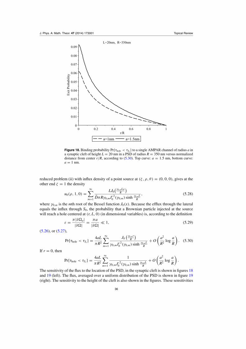
J. Phys. A: Math. Theor. 47 (2014) 173001 Topical Review
Figure 18. Binding probability Pr{τhole < τSr } to a single AMPAR channel of radius a ina synaptic cleft of height L = 20 nm in a PSD of radius R = 350 nm versus normalizeddistance from center r/R, according to (5.30). Top curve: a = 1.5 nm, bottom curve:a = 1 nm.
reduced problem (ii) with influx density of a point source at (ζ , ρ, θ ) = (0, 0, 0), gives at theother end ζ = 1 the density
u0(ρ, 1, 0) =∞∑
m=1
LJ0( γ0,mLρ
R
)DπRγ0,mJ′
02(γ0,m) sinh γ0,mL
R
, (5.28)
where γ0,m is the mth root of the Bessel function J0(x). Because the efflux through the lateralequals the influx through S0, the probability that a Brownian particle injected at the sourcewill reach a hole centered at (r, L, 0) (in dimensional variables) is, according to the definition
ε = π |∂�a||∂�| = πa
|∂�| � 1, (5.29)
(5.26), or (5.27),
Pr{τhole < τSr } = 4aL
πR2
∞∑m=1
J0( γ0,mr
R
)γ0,mJ′
02(γ0,m) sinh γ0,mL
R
+ O
(a2
R2log
a
R
). (5.30)
If r = 0, then
Pr{τhole < τSr } = 4aL
πR2
∞∑m=1
1
γ0,mJ′0
2(γ0,m) sinh γ0,mL
R
+ O
(a2
R2log
a
R
).
The sensitivity of the flux to the location of the PSD, in the synaptic cleft is shown in figures 18and 19 (left). The flux, averaged over a uniform distribution of the PSD is shown in figure 19(right). The sensitivity to the height of the cleft is also shown in the figures. These sensitivities
36

J. Phys. A: Math. Theor. 47 (2014) 173001 Topical Review
Figure 19. Left: binding probability Pr{τhole < τSr } to an AMPA receptor in a cluster of7 in the PSD. Right: the binding probability for 20 AMPA receptors scattered uniformlywithin radius r < R, according (5.30) averaged with respect to the uniform density. Topcurve: L/R = 0.05, bottom curve: L/R = 0.1.
may hint at a possible way of regulating synaptic transmission in the cleft of a neuronalsynapse by changing the location of the PSD or its size (e.g., anchoring more NMDA orAMPA receptors there). Consequently, the probability for a NT to hit the PSD remains verylow and the present computation gives only an upper bound. It was found in Taflia and Holcman(2011), by using a model with a partially absorbing boundary, that the probability to bind toreceptors in the PSD is of the order of 10−3. This is, however, compensated by a large numberof NTs, of the order of 3 103.
5.5. References to section 5
The leakage problem of section 5.3 was solved in Singer et al (2008). The role of cell geometryin controlling the diffusion flux and in determining cell function, as revealed by the microscopicstudies of Harris and Stevens (1988) and Bourne and Harris (2008), is elaborated in Svobodaet al (1996), Korkotian (2004), Hotulainen and Hoogenraad (2010) and Newpher and Ehlers(2009). It is stated in Rosenmund et al (1998) and Gebhardt et al (2006) that AMPA receptorscan bind to a glutamate molecule. However, Jonas et al (1993) reports that two glutamatemolecules are required to open a single AMPA channel. The post-synaptic current depends onthe frequency and location of released vesicles (Madison et al 1991).
The connection of synaptic plasticity to learning and memory is related in Madisonet al (1991). Regulation of synaptic plasticity by geometry is discussed in Korkotian (2004),Majewska et al (2000), Svoboda et al (1996), Biess et al (2007) and Holcman and Kupka(2010). Regulation of the number and type of receptors that contribute to the shaping ofthe synaptic current is discussed in Bredt and Nicoll (2003), Shi et al (1999), Malinow andMalenka (2002), Choquet and Borgdorff (2002), Triller and Choquet (2003), Holcman andTriller (2006) and Holcman et al (2005a).
37
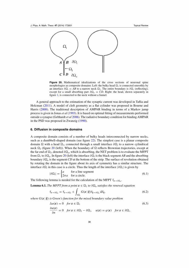
J. Phys. A: Math. Theor. 47 (2014) 173001 Topical Review
Figure 20. Mathematical idealizations of the cross sections of neuronal spinemorphologies as composite domains: Left: the bulky head �1 is connected smoothly byan interface ∂�i = AB to a narrow neck �2. The entire boundary is ∂�r (reflecting),except for a small absorbing part ∂�a = CD. Right: the head, shown separately infigure 1, is connected to the neck without a funnel.
A general approach to the estimation of the synaptic current was developed in Taflia andHolcman (2011). A model of cleft geometry as a flat cylinder was proposed in Bourne andHarris (2008). The traditional description of AMPAR binding in terms of a Markov jumpprocess is given in Jonas et al (1993). It is based on optimal fitting of measurements performedoutside a synapse (Gebhardt et al 2006). The radiative boundary condition for binding AMPARin the PSD was proposed in Zwanzig (1990).
6. Diffusion in composite domains
A composite domain consists of a number of bulky heads interconnected by narrow necks,such as a dumbbell-shaped domain (see figure 22). The simplest case is a planar compositedomain � with a head �1, connected through a small interface ∂�i to a narrow cylindricalneck �2 (figure 20 (left)). When the boundary of � reflects Brownian trajectories, except atthe far end of �2, denoted ∂�a, which is absorbing, the NET problem is to evaluate the MFPTfrom �1 to ∂�a. In figure 20 (left) the interface ∂�i is the black segment AB and the absorbingboundary ∂�a is the segment CD at the bottom of the strip. The surface of revolution obtainedby rotating the domain in the figure about its axis of symmetry has a similar structure. Theinterface ∂�i in this case is a circle. Thus the length of the interface |∂�i| is given by
|∂�i| ={
a for a line segment2πa for a circle.
(6.1)
The following lemma is needed for the calculation of the MFPT τx→∂�a .
Lemma 6.1. The MFPT from a point x ∈ �1 to ∂�a satisfies the renewal equation
τx→∂�a = τx→∂�i +∫
∂�i
G(x | ξ)τξ→∂�a dSξ, (6.2)
where G(x | ξ) is Green’s function for the mixed boundary value problem
u(x) = 0 for x ∈ �1 (6.3)
∂u(x)
∂n= 0 for x ∈ ∂�1 − ∂�i, u(x) = ϕ(x) for x ∈ ∂�i.
38
J. Phys. A: Math. Theor. 47 (2014) 173001 Topical Review
Proof. The identity follows from the fact that both sides of (6.2) satisfy (6.3) for x ∈ �1 andcoincide on ∂�i. �
The identity (6.2) can be interpreted as
τx→∂�a = τx→∂�i + τ∂�i→∂�a , (6.4)
where the MFPT τ∂�i→∂�a is τx→∂�a , averaged over ∂�i with respect to the flux density ofBrownian trajectories in �1 into an absorbing boundary at ∂�i (see Schuss 2010b for furtherdetails).
Theorem 6.2 (The NET from a domain with a long neck). The MFPT of Brownian motionfrom a composite domain � with reflecting boundary to an absorbing boundary at the end ofa narrow cylindrical neck of length L is given by
τx→∂�a = τx→∂�i + L2
2D+ |�1|L
|∂�a|D . (6.5)
Proof. Consider the domain � in figure 20. Lemma 6.1 indicates how to sum the MFPTs. Tocalculate τ∂�i→∂�a and the absorption flux at the interface the boundary value problem
v(x) = − 1
Dfor x ∈ � (6.6)
v(x) = 0 for x ∈ ∂�a (6.7)
∂v(x)
∂n(x)= 0 for x ∈ ∂�r (6.8)
has to be solved in the narrow neck �2. The solution can be approximated by that of theone-dimensional boundary value problem
Duzz = −1 for 0 < z < L, u(0) = 0, u(L) = uH,
where the value at the interface u(L) = uH is yet unknown. The solution is given by
u(z) = − z2
2D+ Bz, (6.9)
so that
u(L) = uH = − L2
2D+ b.l., (6.10)
where b.l. is a boundary layer term. Equation (6.10) relates the unknown constants B anduH . The constant B is found by multiplying equation (6.6) by the Neumann function N(x, y),integrating over �1, applying Green’s formula, and using the boundary conditions (6.7) and(6.8). Specifically, we obtain for all y ∈ ∂�i
v(y) = − 1
D
∫�1
N(x, y) dx −∫
∂�i
N(x, y)∂v(x)
∂ndSx + 1
|�1|∫
�1
v(x) dx. (6.11)
Approximating, as we may, v(y) ≈ u(L) and using (6.10) gives
− L2
2D+ b.l. = −1
D
∫�1
N(x, y) dx−∫
∂�i
N(x, y)∂v(x)
∂ndSx + 1
|�1|∫
�1
v(x) dx. (6.12)
Because v(x) is the solution of the boundary value problem (6.6)–(6.8) in the entire domain� = �1
⋃�2, the meaning of (6.12) is the connecting rule (6.4), where
τx→∂�a = 1
|�1|∫
�1
v(x) dx (6.13)
39
J. Phys. A: Math. Theor. 47 (2014) 173001 Topical Review
τ∂�i→∂�a = u(L) (6.14)
τx→∂�i = − 1
D
∫�
N(x, y) dx −∫
∂�i
N(x, y)∂v(x)
∂ndSx. (6.15)
Equation (6.13) gives the MFPT, averaged over �1. The averaging is a valid approximation,because the MFPT to ∂�i is constant to begin with (except in a negligible boundary layer).Equation (6.14) is the MFPT from the interface to the absorbing end ∂�a of the strip, and(6.15) follows from the identity (Singer et al 2006c, Schuss 2013, Holcman and Schuss 2014)
0 = 1
D
∫�
N(x, ξ) dx +∫
∂�a
N(x, ξ)g(x) dSx + Cε, (6.16)
for all ξ ∈ ∂�a. Matching the solutions in �1 and �2 continuously across ∂�i, the total fluxon ∂�i is obtained as
J = D∫
∂�i
∂v(x)
∂νdSx = − (|�1| + |�2|) . (6.17)
Noting that ∂v(x)/∂n = −u′(0) = −B, equations (6.1) and (6.17) give that
B = −
⎧⎪⎪⎪⎪⎪⎪⎨⎪⎪⎪⎪⎪⎪⎩
|�1|aD
+ L
Dfor a line segment
|�1|2πaD
+ L
Dfor a circle
|�1|πa2D
+ L
Dfor a circular disk.
(6.18)
Finally, equations (6.4)–(6.18) give (6.5). The NET τx→∂�i for the various domains is given inHolcman and Schuss (2014). �
Expression (6.5) for the NET from a two-dimensional domain with a bottleneck in theform of one-dimensional neck, such as a dendritic spine (figure 20 (left)), can be phrased asfollows. Consider a domain � with head �1 and a narrow cylindrical neck �2 of length L andradius a. The radius of curvature at the bottleneck in a smooth connecting funnel is Rc. Thefollowing classification of the NET from a dendritic spine holds (figure 21),
τx→∂�a =
⎧⎪⎪⎪⎪⎪⎪⎪⎪⎪⎪⎪⎪⎪⎪⎪⎪⎪⎪⎪⎪⎪⎪⎪⎨⎪⎪⎪⎪⎪⎪⎪⎪⎪⎪⎪⎪⎪⎪⎪⎪⎪⎪⎪⎪⎪⎪⎪⎩
|�1|πD
ln|∂�1|
a+ O(1)
D+ L2
2D+ |�1|L
aDplanar spine connected to the neck at a right angle
π |�1|D
√Rc
a(1 + o(1)) + L2
2D+ |�1|L
2πaDplanar spine with a smooth connecting funnel
|�1|2πD
logsin θ
2
sin δ2
+ L2
2D+ |�1|L
2πaD
spherical spine connected to the neck at a right angle
|�1|2D
(ε�
)−α/1+α2α/1+α
(1 + α) sin π1+α
+ L2
2D+ |�1|L
2πaD
spherical spine with a smooth connecting funnel,
(6.19)
where R is the radius of the sphere, a = R sin δ/2, and θ is the initial elevation angle on thesphere. If |�1| � aL and L � a, the last term in (6.19) is dominant, which is the manifestationof the many returns of Brownian motion from the neck to the head prior to absorption at ∂�a
(see an estimate in Biess et al 2007). Formula (6.19) is used to estimate the residence time ofreceptors on the surface of a dendritic spine. A generalization to three dimensions is given inHolcman and Schuss (2012).
40

J. Phys. A: Math. Theor. 47 (2014) 173001 Topical Review
Figure 21. Receptor movement on the neuronal membrane.
Figure 22. A dumbbell-shaped domain consists of two large compartments �1 and �3
connected by a narrow neck �2. The bottleneck is the interval AB.
6.1. Transition rate and the principal eigenvalue in composite domains
Consider, for simplicity, the sojourn time of Brownian motion in a compartment interconnectedby a narrow neck to another compartment in a composite domain, as shown in figure 22. Thesojourn time is the MFPT from that compartment to another one. In the limit of shrinking neck,the sojourn time is to leading order independent of the initial point of the escaping trajectoryand equals twice the MFPT from the compartment to the narrowest passage in the bottleneck(e.g., the interval AB in figure 22). Indeed, the reciprocal of this MFPT is to leading order therate at which trajectories reach the bottleneck from the first compartment, so the reciprocal ofthe MFPT is the lowest eigenvalue of the mixed Neumann–Dirichlet boundary value problemin the first compartment with Dirichlet conditions on the cross section of the neck.
There is a spectral gap of order one from the smallest eigenvalue to the next one. Thus, itfollows that long transition times of Brownian trajectories between compartments connected by
41
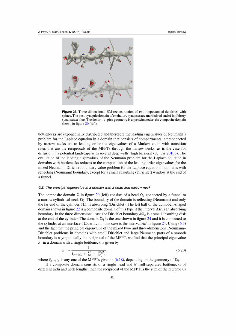
J. Phys. A: Math. Theor. 47 (2014) 173001 Topical Review
Figure 23. Three-dimensional EM reconstruction of two hippocampal dendrites withspines. The post-synaptic domain of excitatory synapses are marked red and of inhibitorysynapses m blue. The dendritic spine geometry is approximated as the composite domainshown in figure 20 (left).
bottlenecks are exponentially distributed and therefore the leading eigenvalues of Neumann’sproblem for the Laplace equation in a domain that consists of compartments interconnectedby narrow necks are to leading order the eigenvalues of a Markov chain with transitionrates that are the reciprocals of the MFPTs through the narrow necks, as is the case fordiffusion in a potential landscape with several deep wells (high barriers) (Schuss 2010b). Theevaluation of the leading eigenvalues of the Neumann problem for the Laplace equation indomains with bottlenecks reduces to the computation of the leading order eigenvalues for themixed Neumann–Dirichlet boundary value problem for the Laplace equation in domains withreflecting (Neumann) boundary, except for a small absorbing (Dirichlet) window at the end ofa funnel.
6.2. The principal eigenvalue in a domain with a head and narrow neck
The composite domain � in figure 20 (left) consists of a head �1 connected by a funnel toa narrow cylindrical neck �2. The boundary of the domain is reflecting (Neumann) and onlythe far end of the cylinder ∂�a is absorbing (Dirichlet). The left half of the dumbbell-shapeddomain shown in figure 22 is a composite domain of this type if the interval AB is an absorbingboundary. In the three-dimensional case the Dirichlet boundary ∂�a is a small absorbing diskat the end of the cylinder. The domain �1 is the one shown in figure 24 and it is connected tothe cylinder at an interface ∂�i, which in this case is the interval AB in figure 24. Using (6.5)and the fact that the principal eigenvalue of the mixed two- and three-dimensional Neumann–Dirichlet problems in domains with small Dirichlet and large Neumann parts of a smoothboundary is asymptotically the reciprocal of the MFPT, we find that the principal eigenvalueλ1 in a domain with a single bottleneck is given by
λ1 ∼ 1
τx→∂�i + L2
2D + |�1|L|∂�a|D
, (6.20)
where τx→∂�i is any one of the MFPTs given in (6.18), depending on the geometry of �1.If a composite domain consists of a single head and N well-separated bottlenecks of
different radii and neck lengths, then the reciprocal of the MFPT is the sum of the reciprocals
42
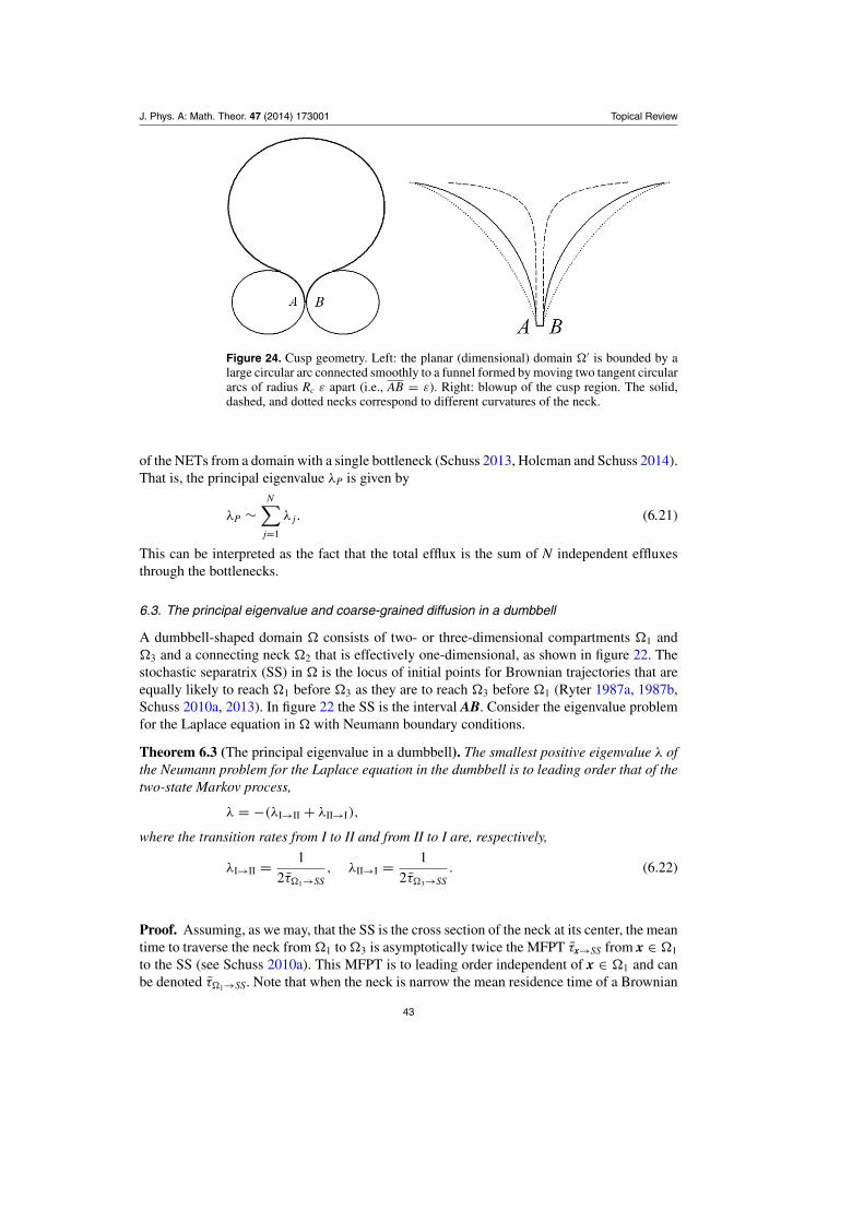
J. Phys. A: Math. Theor. 47 (2014) 173001 Topical Review
Figure 24. Cusp geometry. Left: the planar (dimensional) domain �′ is bounded by alarge circular arc connected smoothly to a funnel formed by moving two tangent circulararcs of radius Rc ε apart (i.e., AB = ε). Right: blowup of the cusp region. The solid,dashed, and dotted necks correspond to different curvatures of the neck.
of the NETs from a domain with a single bottleneck (Schuss 2013, Holcman and Schuss 2014).That is, the principal eigenvalue λP is given by
λP ∼N∑
j=1
λ j. (6.21)
This can be interpreted as the fact that the total efflux is the sum of N independent effluxesthrough the bottlenecks.
6.3. The principal eigenvalue and coarse-grained diffusion in a dumbbell
A dumbbell-shaped domain � consists of two- or three-dimensional compartments �1 and�3 and a connecting neck �2 that is effectively one-dimensional, as shown in figure 22. Thestochastic separatrix (SS) in � is the locus of initial points for Brownian trajectories that areequally likely to reach �1 before �3 as they are to reach �3 before �1 (Ryter 1987a, 1987b,Schuss 2010a, 2013). In figure 22 the SS is the interval AB. Consider the eigenvalue problemfor the Laplace equation in � with Neumann boundary conditions.
Theorem 6.3 (The principal eigenvalue in a dumbbell). The smallest positive eigenvalue λ ofthe Neumann problem for the Laplace equation in the dumbbell is to leading order that of thetwo-state Markov process,
λ = −(λI→II + λII→I),
where the transition rates from I to II and from II to I are, respectively,
λI→II = 1
2τ�1→SS, λII→I = 1
2τ�3→SS. (6.22)
Proof. Assuming, as we may, that the SS is the cross section of the neck at its center, the meantime to traverse the neck from �1 to �3 is asymptotically twice the MFPT τx→SS from x ∈ �1
to the SS (see Schuss 2010a). This MFPT is to leading order independent of x ∈ �1 and canbe denoted τ�1→SS. Note that when the neck is narrow the mean residence time of a Brownian
43

J. Phys. A: Math. Theor. 47 (2014) 173001 Topical Review
trajectory in �1 or in �3 is much longer than that in �2. Also note that the first passage timeτx→SS for x ∈ �1 is exponentially distributed for long times and so is τx→SS for x ∈ �3 (Schuss2010b). Therefore the Brownian motion in � can be coarse-grained into a two-state Markovprocess (a telegraph process), which is in State I when the Brownian trajectory is in �1 and isin State II when it is in �3. The state �2 and the residence time there can be neglected relativeto those in �1 and �3. The transition rates from I to II and from II to I, given in (6.22), canbe found from (6.20), with L half the length of the neck and SS = ∂�a. The radii of curvatureRc,1 and Rc,3 at the two funnels may be different, and the domain is either �1 or �3, as thecase may be.
The asymmetric Markovian random telegraph process jumps between two states, I and II,at independent exponentially distributed waiting times with rates λI→II and λII→I, respectively.The transition probability distribution function satisfies the linear differential equations6
(Schuss 2010b)dP{I, t | x, t0}
dt= −λI→IIP{I, t | x, t0} + λII→IP{II, t | x, t0}
dP{II, t | x, t0}dt
= λI→IIP{I, t | x, t0} − λII→IP{II, t | x, t0}, (6.23)
which can be written in the obvious matrix notation as p = Ap with
A =(−λI→II λII→I
λI→II −λII→I
).
The eigenvalues of A are 0 with the normalized eigenvector ( 12 , 1
2 )T , and −(λI→II + λII→I)
with the eigenvector (1,−1)T . It follows that the nonzero eigenvalue of the system (6.23) isλ = λI→II + λII→I. Hence the theorem follows. �
For example, if the solid dumbbell consists of two general heads connected smoothly tothe neck by funnels, the two rates are given by (Schuss 2013, Holcman and Schuss 2014)
1
λI�II=
√2
[(Rc,1/3
a
)3/2 |�1/3|Rc,1/3D
][1 + o(1)] + L2
4D+ |�1/3|L
πa2D. (6.24)
Consider, for example, the Neumann problem for the Laplace equation in a domain thatconsists of any number of heads interconnected by narrow necks. The Brownian motion canbe coarse-grained into a Markovian random walk that jumps between the connected domainsat exponentially distributed times with rates determined by the first passage times and exitprobabilities, as described in section 6.2. This random walk can in turn be approximated by aneffective coarse-grained anisotropic diffusion, as done, for example, for atomic migration incrystals (Schuss 1980, chapter 8, section 2), for effective diffusion on a surface with obstacles(see section 3.1 and (Holcman et al 2011)), and for a general diffusion on a potential landscapewith deep wells (Hanggi et al 1990).
Some estimates of the asymptotic behavior of the leading eigenvalue in dumbbell-shapeddomains are given in Arrieta (1995), Ward and Stafford (1999), Jimbo and Kosugi (2009),Dagdug et al (2003), and references therein.
6.4. Diffusional transfer of genetic material during cell division
During cell division, daughter and mother cells remain connected by a neck that grows narrowuntil it breaks off. The two connected cells have the shape of an asymmetric dumbbell. Duringthis division process, some of the genetic (mRNA and TFs) material is delivered from the
6 see http://en.wikipedia.org/wiki/Telegraph_process.
44

J. Phys. A: Math. Theor. 47 (2014) 173001 Topical Review
mother to the daughter cell. It remains unclear how this genetic material is selected. A recentreport (Gehlen et al 2011) proposes that diffusion through the connecting neck is the maindeterminant of the delivery rate and of the selection of fast diffusing particles during thetransient regime, before steady state is reached. The effect of asymmetry in the curvatureof the connecting neck in the dumbbell can be analyzed in the limit of a narrow neck. Thetransition rates between the two cells can differ by orders of magnitude as the geometrychanges. This can be used to re-interpret the findings reported experimentally in Gehlen et al(2011).
7. Summary and discussion
This review presents recent progress in stochastic modeling in cellular biology and in coarse-graining molecular-level models of Brownian motion in biological cells or on their membranesinto the cellular scale, where cell function can be discerned. The key factor in this coarse-graining is the time scale of passage time through narrow necks. The passage through smallopenings or narrow passages emerges as the main flux-controlling machinery on the cellularlevel. The coarse-grained models are used to analyze and simulate models of subcellularprocesses, to quantify their biological functions, and are the basis for data analysis. Theanalytical details of the asymptotic expansion of the narrow escape theory (NET) are reviewedin Holcman and Schuss (2014) and Schuss (2013).
The models and analysis presented here can be extended in several directions. The theoryof threshold in chemical reactions can be used to quantify checkpoint processes in biology,such as the induction of plasticity (Dao Duc and Holcman 2010), the decision to start spindleseparation during cell replication (Dao Duc and Holcman 2012) or any other decision processthat occurs when a certain number of molecules are activated. The model of virus traffickingcan be extended to enveloped viruses. Other steps of viral infection should be further modeled,such as the insertion of the genetic material to a DNA site, the synthesis part, the formation ofthe capsid and budding. Another direction is the search for a promoter site in the cell nucleus.Indeed, a key feature in the search by a TF is the local structure of the DNA conformation andchromatin near the specific binding site. So far no modeling approach has been proposed thatintegrates the DNA organization into the algorithm for estimating of the mean time to find theDNA promoter site. It would be interesting to combine polymer dynamics in microdomainswith the NET. The methodology presented here can be applied to the modeling of synaptictransmission and extended to include various molecular feedbacks implied in modulating theprobability of vesicular release.
Acknowledgment
This research is supported by an ERC-starting-Grant.
References
Abe A, Miyanohara A and Friedmann T 1998 Enhanced gene transfer with fusogenic liposomescontaining vesicular stomatitis virus G glycoprotein J. Virol. 72 6159–63
Alberts B, Bray D, Lewis J, Raff M, Roberts K and Watson J D 1994 Molecular Biology of the Cell(New York: Garland)
Amitai A and Holcman D 2013 Polymer model with long-range interactions: analysis and applicationsto the chromatin structure Phys. Rev. E 88 052604
Amitai A, Kantor Y and Kardar M 2010 First-passage distributions in a collective model of anomalousdiffusion with tunable exponent Phys. Rev. E 81 011107
45

J. Phys. A: Math. Theor. 47 (2014) 173001 Topical Review
Amoruso C, Lagache T and Holcman D 2011 Modeling the early steps of cytoplasmic trafficking in viralinfection and gene delivery SIAM. J. Appl. Math. 71 2334–58
Arrieta J M 1995 Rates of eigenvalues on a dumbbell domain. Simple eigenvalue case Trans. Am. Math.Soc. 347 3503–31
Barkai E, Garini Y and Metzler R 2012 Strange kinetics of single molecules in living cells Phys.Today 65 29
Benichou O, Coppey M, Moreau M, Suet P H and Voituriez R 2005 A stochastic model for intermittentsearch strategies J. Phys.: Condens. Matter 17 4275–86
Berezhkovskii A M and Barzykin A V 2012 Search for a small hole in a cavity wall by intermittent bulkand surface diffusion J. Chem. Phys. 136 054115
Biess A, Korkotian E and Holcman D 2007 Diffusion in a dendritic spine: the role of geometry Phys.Rev. E 76 021922
Bloodgood B L and Sabatini B L 2005 Neuronal activity regulates diffusion across the neck of dendriticspines Science 310 866–9
Borgdorff A J and Choquet D 2002 Regulation of AMPA receptor lateral movements Nature 417 649–53Bourne J N and Harris K M 2008 Balancing structure and function at hippocampal dendritic spines Annu.
Rev. Neurosci. 31 47–67Bouzigues C, Morel M, Triller A and Dahan M 2007 Asymmetric redistribution of GABA receptors
during GABA gradient sensing by nerve growth cones analyzed by single quantum dot imagingProc. Natl Acad. Sci. USA 104 11251–6
Bouzigues C, Holcman D and Dahan M 2010 A mechanism for the polarity formation of chemoreceptorsat the growth cone membrane for gradient amplification during directional sensing PLoSOne 5 e9243
Brandenburg B and Zhuang X 2007 Virus trafficking—learning from single-virus tracking Nature Rev.Microbiol. 5 197–208
Bredt D S and Nicoll R A 2003 AMPA receptor trafficking at excitatory synapses Neuron 40 361–79Bressloff P C and Earnshaw B A 2009 A dynamical corral model of protein trafficking in spines Biophys.
J. 96 1786–802Bressloff P C and Newby J M 2013 Stochastic models of intracellular transport Rev. Mod. Phys. 85 135Burger M, Eisenberg R S and Engl H W 2007 Inverse problems related to ion channel selectivity SIAM
J. Appl. Math. 67 960–89Chen D P, Lear J and Eisenberg R S 1997 Permeation through an open channel: Poisson–Nernst–Planck
theory of a synthetic ionic channel Biophys. J. 72 97–116Choquet D 2010 Fast AMPAR trafficking for a high-frequency synaptic transmission Eur. J.
Neurosci. 32 250–60Choquet D and Borgdorff A J 2002 Regulation of AMPA receptor lateral movements Nature 417 649–53Coppey M, Benichou O, Voituriez R and Moreau M 2004 Kinetics of target site localization of a protein
on DNA: a stochastic approach Biophys. J. 87 1640–9Cowan W M, Sudhof T C and Stevens C F (ed) 2003 Synapses (Baltimore, MD: Johns Hopkins University
Press)Dagdug L, Berezhkovskii A M, Shvartsman S Y and Weiss G H 2003 Equilibration in two chambers
connected by a capillary J. Chem. Phys. 119 12473–8Dao Duc K and Holcman D 2010 Threshold activation for stochastic chemical reactions in microdomains
Phys. Rev. E 81 041107Dao Duc K and Holcman D 2012 Using default constraints of the spindle assembly checkpoints to
estimate the associate chemical rates BMC Biophys. 5 1Dauty E and Verkman A S 2005 Actin cytoskeleton as the principal determinant of size-dependent DNA
mobility in cytoplasm: a new barrier for non-viral gene delivery J. Biol. Chem. 280 7823–8Doering C 2000 Effect of boundary condition fluctuations on Smoluchowski reaction rates Stochastic
Processes in Physics, Chemistry, and Biology Lecture Notes in Physics vol 557 (New York: Springer)pp 316–26
Edidin M, Kuo S C and Sheetz M P 1991 Lateral movements of membrane glycoproteins restricted bydynamic cytoplasmic barriers Science 254 1379–82
Eisinger J, Flores J and Petersen W P 1986 A milling crowd model for local and long-range obstructedlateral diffusion. Mobility of excimeric probes in the membrane of intact erythrocytes Biophys.J. 49 987–1001
Elf J, Li G and Xie X 2007 Probing transcription factor dynamics at the single-molecule level in a livingcell Science 316 1191
46

J. Phys. A: Math. Theor. 47 (2014) 173001 Topical Review
Fabrikant V I 1989 Applications of Potential Theory in Mechanics (Dodrecht: Kluwer)Fabrikant V I 1991 Mixed Boundary Value Problems of Potential Theory and Their Applications in
Engineering (Dodrecht: Kluwer)Farr G A, Zhang L G and Tattersall P 2005 Parvoviral virions deploy a capsid-tethered lipolytic enzyme
to breach the endosomal membrane during cell entry Proc. Natl Acad. Sci. USA 102 17148–53Freche D, Pannasch U, Rouach N and Holcman D 2011 Synapse geometry and receptor dynamics
modulate synaptic strength PLoS One 6 e25122Furini S, Domene C and Cavalcanti S 2010 Insights into the sliding movement of the lac repressor
nonspecifically bound to DNA J. Phys. Chem. B 114 2238–45Gebhardt C and Cull-Candy S G 2006 Influence of agonist concentration on AMPA and kainate channels
in CA1 pyramidal cells in rat hippocampal slices J. Physiol. 573 371–94Gehlen L R, Nagai S, Shimada K, Meister P, Taddei A and Gasser S M 2011 Nuclear geometry and
rapid mitosis ensure asymmetric episome segregation in yeast Curr. Biol. 21 25–33Gillespie D T 1976 A general method for numerically simulating the stochastic time evolution of coupled
chemical reactions J. Comput. Phys. 22 403–34Greber U F and Way M 2006 A superhighway to virus infection Cell 124 741–54Grigoriev I V, Makhnovskii Y A, Berezhkovskii A M and Zitserman V Y 2002 Kinetics of escape
through a small hole J. Chem. Phys. 116 9574–7Hanggi P, Talkner P and Borkovec M 1990 Rev. Mod. Phys. 62 251–341Harris K M and Stevens J K 1988 Dendritic spines of rat cerebellar purkinje cells: serial electron
microscopy with reference to their biophysical characteristics J. Neurosci. 12 4455–69Hille B 2001 Ionic Channels of Excitable Membranes 3rd edn (Sunderland, MA: Sinauer Associates
Inc.)Hoefling F and Franosch T 2013 Rep. Prog. Phys. 76 046602Holcman D, Hoze N and Schuss Z 2011 Narrow escape through a funnel and effective diffusion on a
crowded membrane Phys. Rev. E 84 021906Holcman D, Korkotian E and Segal M 2005a Calcium dynamics in dendritic spines, modeling and
experiments Cell Calcium 37 467–75Holcman D 2007 Modeling viral and DNA trafficking in the cytoplasm of a cell J. Stat. Phys.
127 471–94Holcman D and Kupka I 2010 Some questions in computational cellular biology J. Fixed Point Theory
Appl. 7 67–83Holcman D, Marchewka A and Schuss Z 2005b The survival probability of diffusion with trapping in
cellular biology Phys. Rev. E 72 031910Holcman D and Schuss Z 2004 Escape through a small opening: receptor trafficking in a synaptic
membrane J. Stat. Phys. 117 191–230Holcman D and Schuss Z 2005 Stochastic chemical reactions in microdomains J. Chem.
Phys. 122 114710Holcman D and Schuss Z 2011 Diffusion laws in dendritic spines J. Math. Neurosci. 1 10Holcman D and Schuss Z 2012 Brownian motion in dire straits SIAM. J. Multiscale Modeling
Simul. 10 1204–31Holcman D and Schuss Z 2014 The narrow escape problem SIAM Rev. at pressHolcman D, Schuss Z and Korkotian E 2004 Calcium dynamics in dendritic spines and spine motility
Biophys. J. 87 81–91Holcman D and Triller A 2006 Modeling synaptic dynamics and receptor trafficking Biophys.
J. 91 2405–15Hotulainen P and Hoogenraad C C 2010 Actin in dendritic spines: connecting dynamics to function
J. Cell Biol. 189 619–29Hoze N, Nair D, Hosy E, Sieben C, Manley S, Herrmann A, Sibarita J B, Choquet D and Holcman D 2012
Heterogeneity of AMPA receptor trafficking and molecular interactions revealed by superresolutionanalysis of live cell imaging Proc. Natl Acad. Sci. USA 109 17052–7
Huang Q, Opitz R, Knapp E W and Herrmann A 2002 Protonation and stability of the globular domainof influenza virus hemagglutinin Biophys. J. 82 1050–8
Jeon J H, Tejedor V, Burov S, Barkai E, Selhuber-Unkel C, Berg-Sorensen K, Oddershede Land Metzler R 2011 In vivo anomalous diffusion and weak ergodicity breaking of lipid granulesPhys. Rev. Lett. 106 048103
Jimbo S and Kosugi S 2009 Spectra of domains with partial degeneration J. Math. Sci. Univ. Tokyo 16269–414
47
J. Phys. A: Math. Theor. 47 (2014) 173001 Topical Review
Jonas P, Major G and Sakmann B 1993 Quantal components of unitary EPSCs at the mossy fibre synapseon CA3 pyramidal cells of a rat hippocampus J. Physiol. 472 615–63
Kandel E R, Schwartz J H and Jessell T M 2000 Principles of Neural Science 4th edn (New York:McGraw-Hill)
Kim S H, Wang W and Kim K K 2002 Dynamic and clustering model of bacterial chemotaxis receptors:structural basis for signaling and high sensitivity Proc. Natl Acad. Sci. USA 99 11611–5
Knessl C, Mangel M, Matkowsky B J and Schuss Z 1984a Solution of Kramers–Moyal equations forproblems in chemical physics J. Chem. Phys. 81 1285–93
Knessl C, Matkowsky B J, Schuss Z and Tier C 1984b An asymptotic theory of large deviations forMarkov jump processes SIAM J. Appl. Math. 45 1006–102
Kolokolnikov T, Titcombe M and Ward M J 2005 Optimizing the fundamental Neumann eigenvalue forthe Laplacian in a domain with small traps Eur. J. Appl. Math. 16 161–200
Korkotian E, Holcman D and Segal M 2004 Dynamic regulation of spine-dendrite coupling in culturedhippocampal neurons Eur. J. Neurosci. 20 2649–63
Kusumi A, Nakada C, Ritchie K, Murase K, Suzuki K, Murakoshi H, Kasai R S, Kondo J and Fujiwara T2005 Paradigm shift of the plasma membrane concept from the two-dimensional continuum fluidto the partitioned fluid: high-speed single-molecule tracking of membrane molecules Annu. Rev.Biophys. Biomol. Struct. 34 351–78
Kusumi A, Sako Y and Yamamoto M 1993 Confined lateral diffusion of membrane receptors as studiedby single particle tracking (nanovid microscopy). Effects of calcium-induced differentiation incultured epithelial cells Biophys. J. 65 2021–40
Lagache T, Danos O and Holcman D 2012 Modeling the step of endosomal escape during cell infectionby a nonenveloped virus Biophys. J. 102 980–9
Lagache T, Dauty E and Holcman D 2009a Physical principles and models describing intracellular virusparticle dynamics Curr. Opin. Microbiol. 12 439–45
Lagache T, Dauty E and Holcman D 2009b Quantitative analysis of virus and plasmid trafficking in cellsPhys. Rev. E 79 011921
Lagache T and Holcman D 2008a Effective motion of a virus trafficking inside a biological cell SIAM.J. Appl. Math. 68 1146–67
Lagache T and Holcman D 2008b Quantifying intermittent transport in cell cytoplasm Phys. Rev.E 77 030901
MacKinnon R 2003 Potassium channels and the atomic basis of selective ion conduction Nobel Lecture2003 www.nobelprize.org/nobel_prizes/chemistry/laureates/2003/mackinnon-lecture.html
Madison D V, Malenka R C and Nicoll R A 1991 Mechanisms underlying long-term potentiation ofsynaptic transmission Annu. Rev. Neurosci. 14 379–397
Majewska A, Brown E, Ross J and Yuste R 2000 Mechanisms of calcium decay kinetics in hippocampalspines: role of spine calcium pumps and calcium diffusion through the spine neck in biochemicalcompartmentalization J. Neurosci. 20 1722–34
Malherbe G and Holcman D 2010 The search for a DNA target in the nucleus Phys. Lett. A374 466–71
Malinow R and Malenka R C 2002 AMPA receptor trafficking and synaptic plasticity Annu. Rev.Neurosci. 25 106–26
Matkowsky B J, Schuss Z, Knessl C, Tier C and Mangel M 1984 Asymptotic solution of the Kramers–Moyal equation and first-passage times for Markov jump processes Phys. Rev. A 29 3359–69
Mattos T G, Meja-Monasterio C, Metzler R, Oshanin G and Schehr G 2012 Trajectory-to-trajectoryfluctuations in first-passage phenomena in bounded domains Phys. Rev. E 86 031143
Nadler B, Naeh T and Schuss Z 2002 The stationary arrival process of diffusing particles from acontinuum to an absorbing boundary is Poissonian SIAM J. Appl. Math. 62 433–47
Newpher T M and Ehlers M D 2009 Spine microdomains for postsynaptic signaling and plasticity TrendsCell Biol. 5 218–27
Oshanin G, Tamm M and Vasilyev O 2010 Narrow-escape times for diffusion in microdomains with aparticle-surface affinity: mean-field results J. Chem. Phys. 132 235101
Popov I Yu 1992 Extension theory and localization of resonances for domains of trap type Math. USSRSb. 71 209–34
Rachakonda P S, Veit M, Korte T, Ludwig K, Bottcher C, Huang Q, Schmidt M F G and Herrmann A2007 The relevance of salt bridges for the stability of the influenza virus hemagglutinin FASEBJ. 21 995–1002
Rayleigh J W S 1945 The Theory of Sound vol 2 2nd edn (New York: Dover)
48
J. Phys. A: Math. Theor. 47 (2014) 173001 Topical Review
Reingruber J, Abad E and Holcman D 2009 Narrow escape time to a structured target located at theboundary of a microdomian J. Chem. Phys. 130 094909
Reingruber J and Holcman D 2009 The gated narrow escape time for molecular signaling Phys. Rev.Lett. 103 148102
Reingruber J and Holcman D 2010 Narrow escape for a stochastically gated Brownian ligand J. Phys.:Condens. Matter 22 065103
Reingruber J and Holcman D 2011a The narrow escape problem in a flat cylindrical microdomain, withapplication to diffusion in the synaptic cleft Multiscale Modeling Simul. 9 793–816
Reingruber J and Holcman D 2011b Transcription factor search for a DNA promoter in a three-statemodel Phys. Rev. E 84 020901
Renner M, Choquet D and Triller A 2009 Control of the postsynaptic membrane viscosityJ. Neurosci. 29 2926–637
Rosenmund C, Stern-Bach Y and Stevens C F 1998 The tetrameric structure of a glutamate receptorchannel Science 280 1596–9
Ryter D 1987a Noise-induced transitions in a double-well potential at low friction J. Stat. Phys. 49 751–65Ryter D 1987b On the eigenfunctions of the Fokker–Planck operator and of its adjoint Physica
A 142 103–21Sakmann B and Neher E 2010 Single-Channel Recording (New York: Springer)Saxton M J 1995 Single-particle tracking: effects of corrals Biophys. J. 69 389–98Saxton M J and Jacobson K 1997 Single-particle tracking: applications to membrane dynamics Annu.
Rev. Biophys. Biomol. Struct. 26 373–99Schuss Z 1980 Theory and Applications of Stochastic Differential Equations (New York: Wiley)Schuss Z 2010a Equilibrium and recrossings of the transition state: What can be learned from diffusion?
J. Phys. Chem. C 114 20320–34Schuss Z 2010b Theory and Applications of Stochastic Processes, and Analytical Approach Applied
Mathematical Sciences vol 170 (New York: Springer)Schuss Z 2013 Brownian Dynamics at Boundaries and Interfaces in Physics, Chemistry, and Biology
(Applied Mathematical Sciences) (New York: Springer)Schuss Z, Singer A and Holcman D 2007 The narrow escape problem for diffusion in cellular
microdomains Proc. Natl Acad. Sci. USA 104 16098–103Schuss Z and Spivak A 2005 On recovering the shape of a domain from the trace of the heat kernel SIAM
J. Appl. Math. 66 339–60Segal M and Andersen P 2000 Dendritic spines shaped by synaptic activity Curr. Opin.
Neurobiol. 10 582–6Seisenberger G, Ried M U, Endress T, Bruning H, Hallek M and Brauchle 2001 Real-time single-
molecule imaging of the infection pathway of an adeno-associated virus Science 294 1929–32Sheetz M P 1993 Glycoprotein motility and dynamic domains in fluid plasma membranes Annu. Rev.
Biophys. Biomol. Struct. 22 417–31Shi S H, Hayashi Y, Petralia R S, Zaman S H, Wenthold R J, Svoboda K and Malinow R 1999 Rapid
spine delivery and redistribution of AMPA receptors after synaptic NMDA receptor activationScience 284 1811–6
Singer A, Schuss Z and Holcman D 2006a Narrow escape. Part II. The circular disk J. Stat.Phys. 122 465–89
Singer A, Schuss Z and Holcman D 2006b Narrow escape: part III. Non-smooth domains and Riemannsurfaces J. Stat. Phys. 122 491–509
Singer A, Schuss Z and Holcman D 2008 Narrow escape and leakage of Brownian particles Phys. Rev.E 78 051111
Singer A, Schuss Z, Holcman D and Eisenberg R S 2006c Narrow escape: part I J. Stat. Phys. 122 437–63Spacek J 2002 Synapse and dentric spine: three-dimensional view of effective tandem Psychiatric
Suppl. 3 6 55–60Sodeik B 2000 Mechanisms of viral transport in the cytoplasm Trends Microbiol. 8 465–72Suzuki K and Sheetz M P 2001 Binding of cross-linked glycosylphosphat-idylinositol-anchored proteins
to discrete actin-associated sites and cholesterol-dependent domains Biophys. J. 81 2181–9Svoboda K, Tank D W and Denk W 1996 Direct measurement of coupling between dendritic spines and
shafts Science 272 716–9Tabei S M, Burov S, Kim H Y, Kuznetsov A, Huynh T, Jureller J, Philipson L H, Dinner A R
and Scherer N F 2013 Intracellular transport of insulin granules is a subordinated random walkProc. Natl Acad. Sci. USA 110 4911
49

J. Phys. A: Math. Theor. 47 (2014) 173001 Topical Review
Taflia A and Holcman D 2011 Estimating the synaptic current in a multiconductance AMPA receptormodel Biophys. J. 101 781–92
Tardin C, Cognet L, Bats C, Lounis B and Choquet D 2003 Direct imaging of lateral movements ofAMPA receptors inside synapses Embo J. 22 4656–65
Triller A and Choquet D 2003 The role of receptor diffusion in the organization of the postsynapticmembrane Nature Rev. Neurosci. 4 1251–65
Tsaneva K, Burgo A, Galli T and Holcman D 2009 Quantifying neurite growth mediated by interactionsbetween secretory vesicles, microtubules and actin networks Biophys. J. 96 840–57
Tu Y and Kim J S 2008 A fusogenic segment of glycoprotein H from herpes simplex virus enhancestransfection efficiency of cationic liposomes J. Gene Med. 10 646–54
Verkman A S 2002 Solute and macromolecule diffusion in cellular aqueous compartments TrendsBiochem. Sci. 27 27–33
Von Hippel P and Berg O G 1989 Facilitated target location in biological systems J. Biol. Chem.264 675–8
Wang Y, Austin R and Cox E 2006 Single molecule measurements of repressor protein 1D diffusion onDNA Phys. Rev. Lett. 97 048302
Ward M J and Keller J B 1993 Strong localized perturbations of eigenvalue problems SIAM J. Appl.Math. 53 770–98
Ward M J and Stafford D 1999 Metastable dynamics and spatially inhomogeneous equilibria in dumbell-shaped domains Stud. Appl. Math. 103 51–73
Whittaker G R, Kann M and Helenius A 2000 Viral entry into the nucleus Annu. Rev. Cell Dev.Biol. 16 627–51
Zwanzig R 1990 Diffusion-controlled ligand binding to spheres covered by receptors: an effectivemedium treatment. Proc. Natl Acad. Sci. USA 87 5856–7
50