Embed Size (px)
Citation preview
Introduction P(up) Hidden liquidity Latency Optimal liquidation Conclusion
Time is Money:Estimating the Cost of Latency in Trading
Sasha Stoikov
Cornell University
December 10, 2014
Introduction P(up) Hidden liquidity Latency Optimal liquidation Conclusion
Background
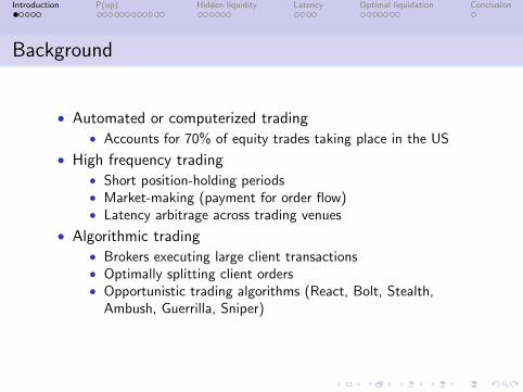
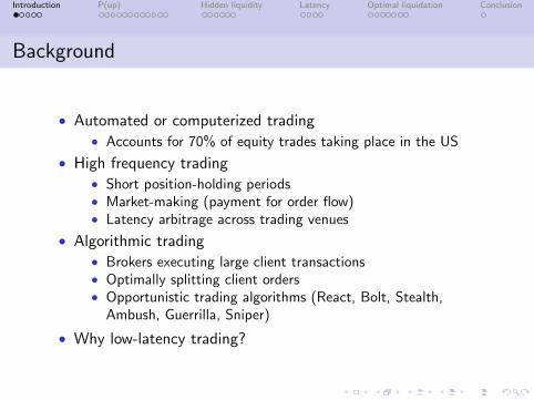
• Automated or computerized trading• Accounts for 70% of equity trades taking place in the US
• High frequency trading
• Short position-holding periods• Market-making (payment for order flow)• Latency arbitrage across trading venues
• Algorithmic trading
• Brokers executing large client transactions• Optimally splitting client orders• Opportunistic trading algorithms (React, Bolt, Stealth,
Ambush, Guerrilla, Sniper)
• Why low-latency trading?

Introduction P(up) Hidden liquidity Latency Optimal liquidation Conclusion
Background
• Automated or computerized trading• Accounts for 70% of equity trades taking place in the US
• High frequency trading• Short position-holding periods• Market-making (payment for order flow)• Latency arbitrage across trading venues
• Algorithmic trading
• Brokers executing large client transactions• Optimally splitting client orders• Opportunistic trading algorithms (React, Bolt, Stealth,
Ambush, Guerrilla, Sniper)
• Why low-latency trading?
Introduction P(up) Hidden liquidity Latency Optimal liquidation Conclusion
Background
• Automated or computerized trading• Accounts for 70% of equity trades taking place in the US
• High frequency trading• Short position-holding periods• Market-making (payment for order flow)• Latency arbitrage across trading venues
• Algorithmic trading• Brokers executing large client transactions• Optimally splitting client orders• Opportunistic trading algorithms (React, Bolt, Stealth,
Ambush, Guerrilla, Sniper)
• Why low-latency trading?
Introduction P(up) Hidden liquidity Latency Optimal liquidation Conclusion
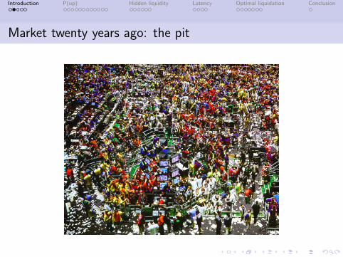
Market twenty years ago: the pit
Introduction P(up) Hidden liquidity Latency Optimal liquidation Conclusion
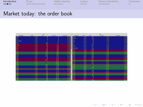
Market today: the order book
Introduction P(up) Hidden liquidity Latency Optimal liquidation Conclusion
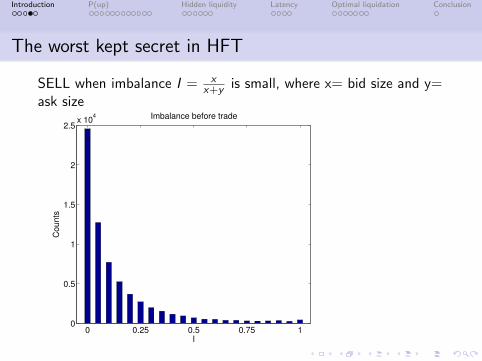
The worst kept secret in HFT
SELL when imbalance I = xx+y is small, where x= bid size and y=
ask size
0 0.25 0.5 0.75 10
0.5
1
1.5
2
2.5x 10
4
I
Co
un
ts
Imbalance before trade
Introduction P(up) Hidden liquidity Latency Optimal liquidation Conclusion
Outline
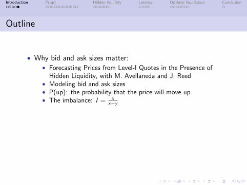
• Why bid and ask sizes matter:• Forecasting Prices from Level-I Quotes in the Presence of
Hidden Liquidity, with M. Avellaneda and J. Reed• Modeling bid and ask sizes• P(up): the probability that the price will move up• The imbalance: I = x
x+y
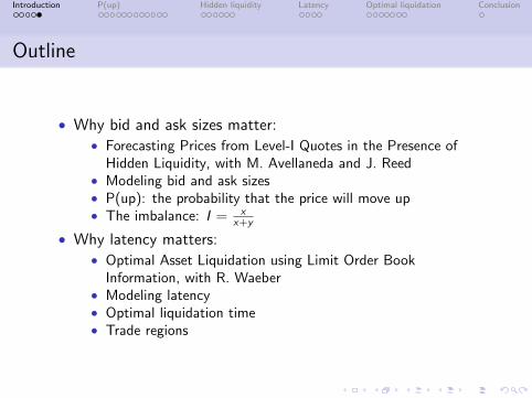
• Why latency matters:
• Optimal Asset Liquidation using Limit Order BookInformation, with R. Waeber
• Modeling latency• Optimal liquidation time• Trade regions
Introduction P(up) Hidden liquidity Latency Optimal liquidation Conclusion
Outline
• Why bid and ask sizes matter:• Forecasting Prices from Level-I Quotes in the Presence of
Hidden Liquidity, with M. Avellaneda and J. Reed• Modeling bid and ask sizes• P(up): the probability that the price will move up• The imbalance: I = x
x+y
• Why latency matters:• Optimal Asset Liquidation using Limit Order Book
Information, with R. Waeber• Modeling latency• Optimal liquidation time• Trade regions
Introduction P(up) Hidden liquidity Latency Optimal liquidation Conclusion
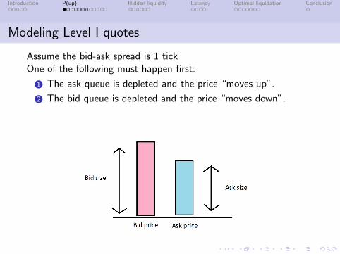
Modeling Level I quotes
Assume the bid-ask spread is 1 tickOne of the following must happen first:
1 The ask queue is depleted and the price “moves up”.
2 The bid queue is depleted and the price “moves down”.
Introduction P(up) Hidden liquidity Latency Optimal liquidation Conclusion
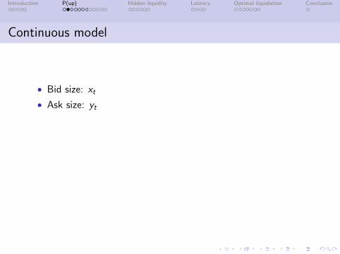
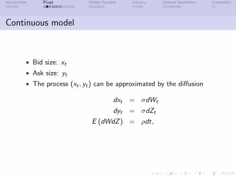
Continuous model
• Bid size: xt
• Ask size: yt
• The process (xt , yt) can be approximated by the diffusion
dxt = σdWt
dyt = σdZt
E (dWdZ ) = ρdt,
• τx and τy are the times when the sizes hit zero
Introduction P(up) Hidden liquidity Latency Optimal liquidation Conclusion
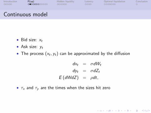
Continuous model
• Bid size: xt
• Ask size: yt
• The process (xt , yt) can be approximated by the diffusion
dxt = σdWt
dyt = σdZt
E (dWdZ ) = ρdt,
• τx and τy are the times when the sizes hit zero
Introduction P(up) Hidden liquidity Latency Optimal liquidation Conclusion
Continuous model
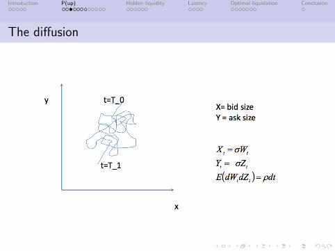
• Bid size: xt
• Ask size: yt
• The process (xt , yt) can be approximated by the diffusion
dxt = σdWt
dyt = σdZt
E (dWdZ ) = ρdt,
• τx and τy are the times when the sizes hit zero
Introduction P(up) Hidden liquidity Latency Optimal liquidation Conclusion
The diffusion
Introduction P(up) Hidden liquidity Latency Optimal liquidation Conclusion
The partial differential equation
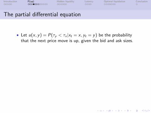
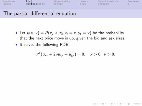
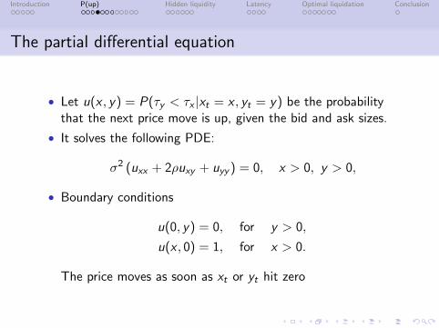
• Let u(x , y) = P(τy < τx |xt = x , yt = y) be the probabilitythat the next price move is up, given the bid and ask sizes.
• It solves the following PDE:
σ2 (uxx + 2ρuxy + uyy ) = 0, x > 0, y > 0,
• Boundary conditions
u(0, y) = 0, for y > 0,
u(x , 0) = 1, for x > 0.
The price moves as soon as xt or yt hit zero
Introduction P(up) Hidden liquidity Latency Optimal liquidation Conclusion
The partial differential equation
• Let u(x , y) = P(τy < τx |xt = x , yt = y) be the probabilitythat the next price move is up, given the bid and ask sizes.
• It solves the following PDE:
σ2 (uxx + 2ρuxy + uyy ) = 0, x > 0, y > 0,
• Boundary conditions
u(0, y) = 0, for y > 0,
u(x , 0) = 1, for x > 0.
The price moves as soon as xt or yt hit zero
Introduction P(up) Hidden liquidity Latency Optimal liquidation Conclusion
Solution
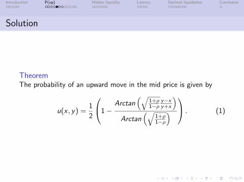
TheoremThe probability of an upward move in the mid price is given by
u(x , y) =1
2
1−Arctan
(√1+ρ1−ρ
y−xy+x
)Arctan
(√1+ρ1−ρ
) . (1)

Introduction P(up) Hidden liquidity Latency Optimal liquidation Conclusion
Uncorrelated queues (ρ = 0)
• Problemuxx + uyy = 0, x > 0, y > 0,
and
u(0, y) = 0, for y > 0,
u(x , 0) = 1, for x > 0.
• Solution
u(x , y) =2
πArctan
(x
y
).

Introduction P(up) Hidden liquidity Latency Optimal liquidation Conclusion
Uncorrelated queues (ρ = 0)
• Problemuxx + uyy = 0, x > 0, y > 0,
and
u(0, y) = 0, for y > 0,
u(x , 0) = 1, for x > 0.
• Solution
u(x , y) =2
πArctan
(x
y
).

Introduction P(up) Hidden liquidity Latency Optimal liquidation Conclusion
Perfectly negatively correlated queues (ρ = −1)
• Problem
uxx − 2uxy + uyy = 0, x > 0, y > 0,
and
u(0, y) = 0, for y > 0,
u(x , 0) = 1, for x > 0.
• Solutionu(x , y) =
x
x + y.

Introduction P(up) Hidden liquidity Latency Optimal liquidation Conclusion
Perfectly negatively correlated queues (ρ = −1)
• Problem
uxx − 2uxy + uyy = 0, x > 0, y > 0,
and
u(0, y) = 0, for y > 0,
u(x , 0) = 1, for x > 0.
• Solutionu(x , y) =
x
x + y.
Introduction P(up) Hidden liquidity Latency Optimal liquidation Conclusion
The data
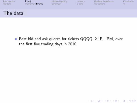
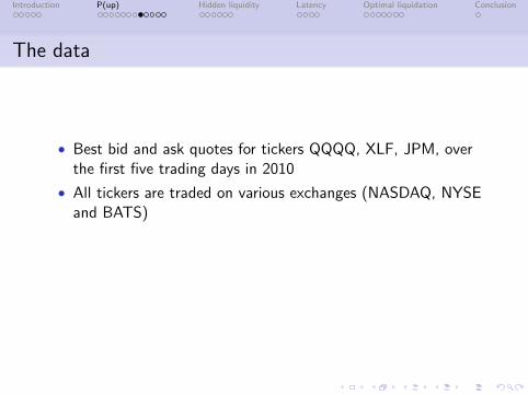
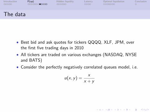
• Best bid and ask quotes for tickers QQQQ, XLF, JPM, overthe first five trading days in 2010
• All tickers are traded on various exchanges (NASDAQ, NYSEand BATS)
• Consider the perfectly negatively correlated queues model, i.e.
u(x , y) =x
x + y
Introduction P(up) Hidden liquidity Latency Optimal liquidation Conclusion
The data
• Best bid and ask quotes for tickers QQQQ, XLF, JPM, overthe first five trading days in 2010
• All tickers are traded on various exchanges (NASDAQ, NYSEand BATS)
• Consider the perfectly negatively correlated queues model, i.e.
u(x , y) =x
x + y
Introduction P(up) Hidden liquidity Latency Optimal liquidation Conclusion
Data sample
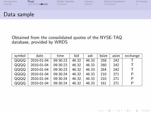
Obtained from the consolidated quotes of the NYSE-TAQdatabase, provided by WRDS
symbol date time bid ask bsize asize exchange
QQQQ 2010-01-04 09:30:23 46.32 46.33 258 242 TQQQQ 2010-01-04 09:30:23 46.32 46.33 260 242 TQQQQ 2010-01-04 09:30:23 46.32 46.33 264 242 TQQQQ 2010-01-04 09:30:24 46.32 46.33 210 271 PQQQQ 2010-01-04 09:30:24 46.32 46.33 210 271 PQQQQ 2010-01-04 09:30:24 46.32 46.33 161 271 P

Introduction P(up) Hidden liquidity Latency Optimal liquidation Conclusion
Summary statistics
Ticker Exchange num qt qt/sec spread bsize+asize price
XLF NASDAQ 0.7M 7 0.010 8797 15.02XLF NYSE 0.4M 4 0.010 10463 15.01XLF BATS 0.4M 4 0.011 7505 14.99
QQQQ NASDAQ 2.7M 25 0.010 1455 46.30QQQQ NYSE 4.0M 36 0.011 1152 46.27QQQQ BATS 1.6M 15 0.011 1055 46.28
JPM NASDAQ 1.2M 11 0.011 87 43.81JPM NYSE 0.7M 6 0.012 47 43.77JPM BATS 0.6M 5 0.014 39 43.82
Table: Summary statistics
Introduction P(up) Hidden liquidity Latency Optimal liquidation Conclusion
Estimation procedure
1 We filter the data set by exchange and ticker
2 We “bucket” the imbalance
I =x
x + y
into intervals: 0 < I ≤ 0.05, 0.05 < I ≤ 0.1, etc..
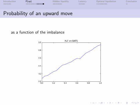
3 For each bucket, we compute the empirical probability thatthe price goes up at the next price move, u(I ).
4 We plot the probability that the next price move is up,conditional on the imbalance.
Introduction P(up) Hidden liquidity Latency Optimal liquidation Conclusion
Estimation procedure
1 We filter the data set by exchange and ticker
2 We “bucket” the imbalance
I =x
x + y
into intervals: 0 < I ≤ 0.05, 0.05 < I ≤ 0.1, etc..
3 For each bucket, we compute the empirical probability thatthe price goes up at the next price move, u(I ).
4 We plot the probability that the next price move is up,conditional on the imbalance.
Introduction P(up) Hidden liquidity Latency Optimal liquidation Conclusion
Probability of an upward move
as a function of the imbalance
Introduction P(up) Hidden liquidity Latency Optimal liquidation Conclusion
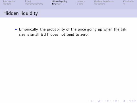
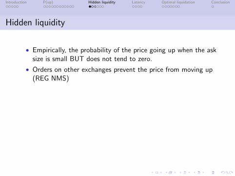
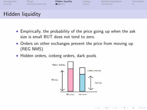
Hidden liquidity
• Empirically, the probability of the price going up when the asksize is small BUT does not tend to zero.
• Orders on other exchanges prevent the price from moving up(REG NMS)
• Hidden orders, iceberg orders, dark pools
Introduction P(up) Hidden liquidity Latency Optimal liquidation Conclusion
Boundary condition
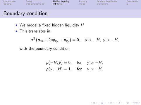
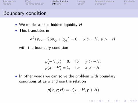
• We model a fixed hidden liquidity H
• This translates in
σ2 (pxx + 2ρpxy + pyy ) = 0, x > −H, y > −H,
with the boundary condition
p(−H, y) = 0, for y > −H,p(x ,−H) = 1, for x > −H.
• In other words we can solve the problem with boundaryconditions at zero and use the relation
p(x , y ;H) = u(x + H, y + H)

Introduction P(up) Hidden liquidity Latency Optimal liquidation Conclusion
Boundary condition
• We model a fixed hidden liquidity H
• This translates in
σ2 (pxx + 2ρpxy + pyy ) = 0, x > −H, y > −H,
with the boundary condition
p(−H, y) = 0, for y > −H,p(x ,−H) = 1, for x > −H.
• In other words we can solve the problem with boundaryconditions at zero and use the relation
p(x , y ;H) = u(x + H, y + H)
Introduction P(up) Hidden liquidity Latency Optimal liquidation Conclusion
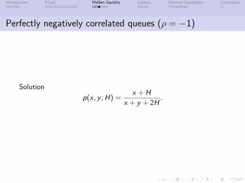
Perfectly negatively correlated queues (ρ = −1)
Solution
p(x , y ;H) =x + H
x + y + 2H.
Introduction P(up) Hidden liquidity Latency Optimal liquidation Conclusion
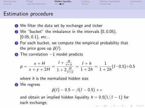
Estimation procedure
1 We filter the data set by exchange and ticker
2 We “bucket” the imbalance in the intervals [0, 0.05),[0.05, 0.1), etc...
3 For each bucket, we compute the empirical probability thatthe price goes up p̂(I ).
4 The correlation −1 model predicts
p =x + H
x + y + 2H=
I + Hx+y
1 + 2 Hx+y
=I + h
1 + 2h=
1
1 + 2h(I−0.5)+0.5
where h is the normalized hidden size
5 We regressp̂(I )− 0.5 = β(I − 0.5) + ε
and obtain an implied hidden liquidity h = 0.5(1/β − 1) foreach exchange.
Introduction P(up) Hidden liquidity Latency Optimal liquidation Conclusion
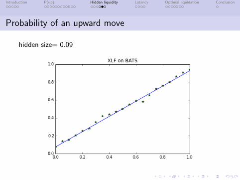
Probability of an upward move
hidden size= 0.09
Introduction P(up) Hidden liquidity Latency Optimal liquidation Conclusion
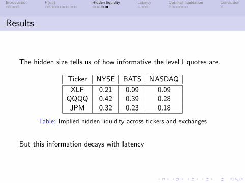
Results
The hidden size tells us of how informative the level I quotes are.
Ticker NYSE BATS NASDAQ
XLF 0.21 0.09 0.09QQQQ 0.42 0.39 0.28
JPM 0.32 0.23 0.18
Table: Implied hidden liquidity across tickers and exchanges
But this information decays with latency
Introduction P(up) Hidden liquidity Latency Optimal liquidation Conclusion
Latency
• Latency arises in every trade execution:
1 Time of datafeed to travel from exchange to executionmachine;
2 The algorithm making a decision;3 The order being sent back to the market.
• We assume there is a fixed latency L
• What you see is not what you get
Introduction P(up) Hidden liquidity Latency Optimal liquidation Conclusion
The cost of latency
There is empirical evidence that selling on small imbalances can beprofitable:
• On each quote i , record the imbalance Ii and the bid price Sbi
• At a later quote in the future j , L milliseconds later, recordthe bid price Sb
j
• Take averages of (Sbj − Sb
i ) for Ii in different buckets
Introduction P(up) Hidden liquidity Latency Optimal liquidation Conclusion
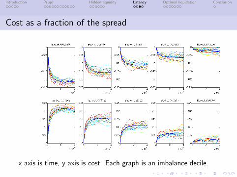
Cost as a fraction of the spread
x axis is time, y axis is cost. Each graph is an imbalance decile.
Introduction P(up) Hidden liquidity Latency Optimal liquidation Conclusion
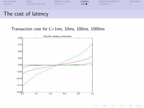
The cost of latency
Transaction cost for L=1ms, 10ms, 100ms, 1000ms
Introduction P(up) Hidden liquidity Latency Optimal liquidation Conclusion
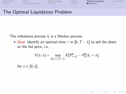
The Optimal Liquidation Problem
The imbalance process It is a Markov process.
• Goal: Identify an optimal time τ in [0,T − L] to sell the shareat the bid price, i.e.,
V (t, x) = sup0≤τ≤T−L
E [Pbτ+L − Pb
0 |It = x ],
for x ∈ [0, 1].
Introduction P(up) Hidden liquidity Latency Optimal liquidation Conclusion
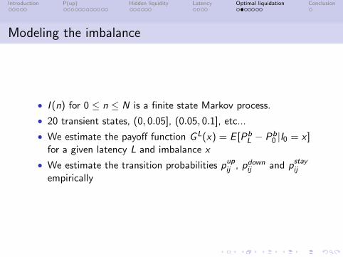
Modeling the imbalance
• I (n) for 0 ≤ n ≤ N is a finite state Markov process.
• 20 transient states, (0, 0.05], (0.05, 0.1], etc...
• We estimate the payoff function GL(x) = E [PbL − Pb
0 |I0 = x ]for a given latency L and imbalance x
• We estimate the transition probabilities pupij , pdownij and pstayij
empirically
Introduction P(up) Hidden liquidity Latency Optimal liquidation Conclusion
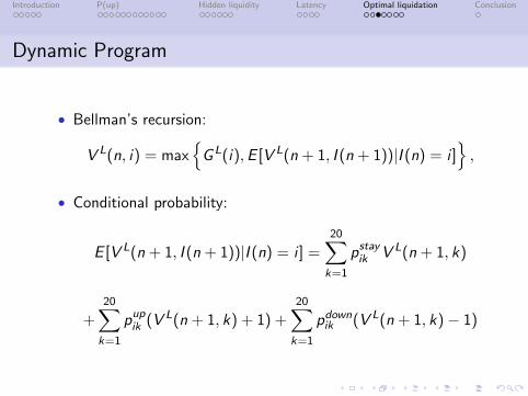
Dynamic Program
• Bellman’s recursion:
V L(n, i) = max{GL(i),E [V L(n + 1, I (n + 1))|I (n) = i ]
},
• Conditional probability:
E [V L(n + 1, I (n + 1))|I (n) = i ] =20∑k=1
pstayik V L(n + 1, k)
+20∑k=1
pupik (V L(n + 1, k) + 1) +20∑k=1
pdownik (V L(n + 1, k)− 1)
Introduction P(up) Hidden liquidity Latency Optimal liquidation Conclusion
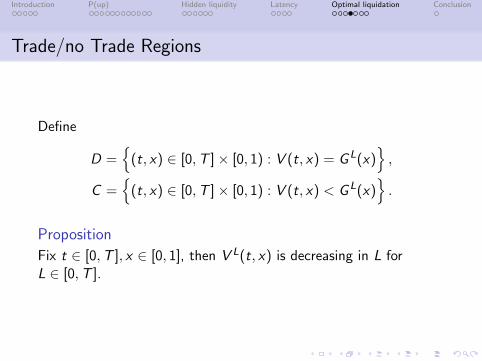
Trade/no Trade Regions
Define
D ={
(t, x) ∈ [0,T ]× [0, 1) : V (t, x) = GL(x)},
C ={
(t, x) ∈ [0,T ]× [0, 1) : V (t, x) < GL(x)}.
Proposition
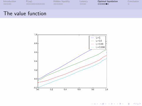
Fix t ∈ [0,T ], x ∈ [0, 1], then V L(t, x) is decreasing in L forL ∈ [0,T ].
Introduction P(up) Hidden liquidity Latency Optimal liquidation Conclusion
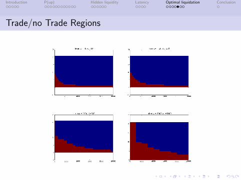
Trade/no Trade Regions
Introduction P(up) Hidden liquidity Latency Optimal liquidation Conclusion
The value function
Introduction P(up) Hidden liquidity Latency Optimal liquidation Conclusion
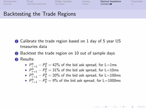
Backtesting the Trade Regions
1 Calibrate the trade region based on 1 day of 5 year UStreasuries data
2 Backtest the trade region on 10 out of sample days
3 Results:• Pb
τ+L − Pb0 = 42% of the bid ask spread, for L=1ms
• Pbτ+L − Pb
0 = 31% of the bid ask spread, for L=10ms• Pb
τ+L − Pb0 = 20% of the bid ask spread, for L=100ms
• Pbτ+L − Pb
0 = 9% of the bid ask spread, for L=1000ms
Introduction P(up) Hidden liquidity Latency Optimal liquidation Conclusion
Conclusion
1 We can estimate the probability of the next price move:• Conditional on the bid and ask sizes• Conditional on imbalance if the sizes are negatively correlated• Conditional on hidden liquidity for a ticker/exchange pair
2 We can estimate the cost of latency:• By solving an optimal stopping problem• Backtesting trade/no trade regions on level I data