Embed Size (px)
Citation preview

Time-headways for interacting particle systemsin stationary state
Pavel Hrabak
UTIA AS8th September 2014
P. Hrabak [email protected] 8th September 2014 1 / 17

Introduction
Scope of the talkinteracting particle systems as traffic flow modelsheadway distributions in IPS
Questions to be answereddistance-headway distribution:
“What is the probability that there is a gap of the length nbetween two consecutive vehicles/particles?”
time-headway distribution
“What is the probability that there is a time interval of the length tbetween the passes of two consecutive vehicles/particles
through a reference point?”
P. Hrabak [email protected] 8th September 2014 2 / 17

IPS in Exclusion Process representation
at most one particle in site x
state of x is τxτx =
{1 x occupied,0 x empty,
particles hopping from x to y with probability/intenzity
p(x, y) · τx ·(1− τy
)· g(τ(Nx,y)
)p(x, y) – underlying random walkg(τ(Nx,y)
)– reaction with the neighbourhood Nx,y
Nx,y
-5 -4 -3 -2 -1 0 1 2 3 4 5 6
p12 p13 p14
P. Hrabak [email protected] 8th September 2014 3 / 17

IPS in Exclusion Process representation
at most one particle in site x
state of x is τxτx =
{1 x occupied,0 x empty,
particles hopping from x to y with probability/intenzity
p(x, y) · τx ·(1− τy
)· g(τ(Nx,y)
)
p(x, y) – underlying random walkg(τ(Nx,y)
)– reaction with the neighbourhood Nx,y
Nx,y
-5 -4 -3 -2 -1 0 1 2 3 4 5 6
p12 p13 p14
P. Hrabak [email protected] 8th September 2014 3 / 17

IPS in Exclusion Process representation
at most one particle in site x
state of x is τxτx =
{1 x occupied,0 x empty,
particles hopping from x to y with probability/intenzity
p(x, y) · τx ·(1− τy
)· g(τ(Nx,y)
)p(x, y) – underlying random walk
g(τ(Nx,y)
)– reaction with the neighbourhood Nx,y
Nx,y
-5 -4 -3 -2 -1 0 1 2 3 4 5 6
p12 p13 p14
P. Hrabak [email protected] 8th September 2014 3 / 17

IPS in Exclusion Process representation
at most one particle in site x
state of x is τxτx =
{1 x occupied,0 x empty,
particles hopping from x to y with probability/intenzity
p(x, y) · τx ·(1− τy
)· g(τ(Nx,y)
)p(x, y) – underlying random walkg(τ(Nx,y)
)– reaction with the neighbourhood Nx,y
Nx,y
-5 -4 -3 -2 -1 0 1 2 3 4 5 6
p12 p13 p14
P. Hrabak [email protected] 8th September 2014 3 / 17

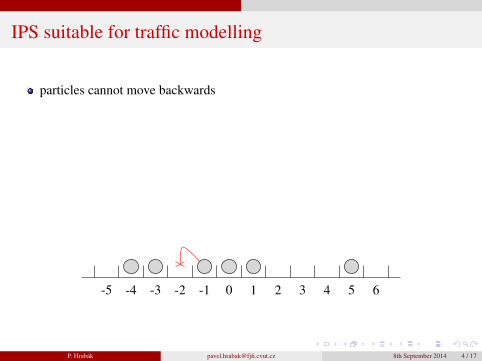
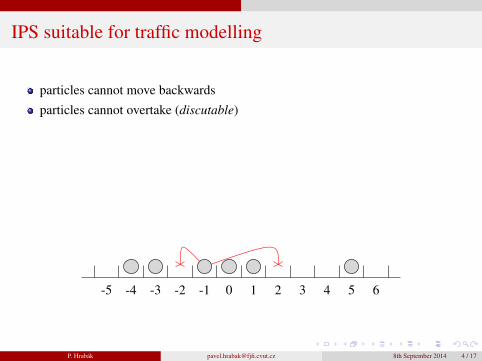
IPS suitable for traffic modelling
particles cannot move backwardsparticles cannot overtake (discutable)the range of Nx,y is “conditionally” restrained (for simplicity)
g(τ(Nx,y)
)= 0⇐
{y < x backward movement∃ z (x < z < y)(τz = 1) overtaking
⊆ N1,y6⊆ N1,y
-5 -4 -3 -2 -1 0 1 2 3 4 5 6
p12 p13 p14
P. Hrabak [email protected] 8th September 2014 4 / 17
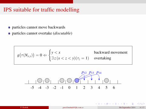
IPS suitable for traffic modelling
particles cannot move backwards
particles cannot overtake (discutable)the range of Nx,y is “conditionally” restrained (for simplicity)
g(τ(Nx,y)
)= 0⇐
{y < x backward movement∃ z (x < z < y)(τz = 1) overtaking
⊆ N1,y6⊆ N1,y
-5 -4 -3 -2 -1 0 1 2 3 4 5 6
p12 p13 p14
P. Hrabak [email protected] 8th September 2014 4 / 17
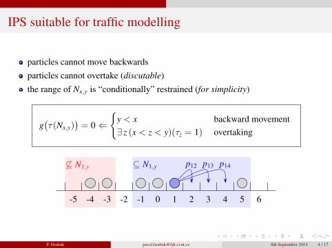
IPS suitable for traffic modelling
particles cannot move backwardsparticles cannot overtake (discutable)
the range of Nx,y is “conditionally” restrained (for simplicity)
g(τ(Nx,y)
)= 0⇐
{y < x backward movement∃ z (x < z < y)(τz = 1) overtaking
⊆ N1,y6⊆ N1,y
-5 -4 -3 -2 -1 0 1 2 3 4 5 6
p12 p13 p14
P. Hrabak [email protected] 8th September 2014 4 / 17
IPS suitable for traffic modelling
particles cannot move backwardsparticles cannot overtake (discutable)the range of Nx,y is “conditionally” restrained (for simplicity)
g(τ(Nx,y)
)= 0⇐
{y < x backward movement∃ z (x < z < y)(τz = 1) overtaking
⊆ N1,y6⊆ N1,y
-5 -4 -3 -2 -1 0 1 2 3 4 5 6
p12 p13 p14
P. Hrabak [email protected] 8th September 2014 4 / 17

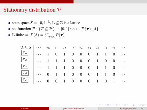
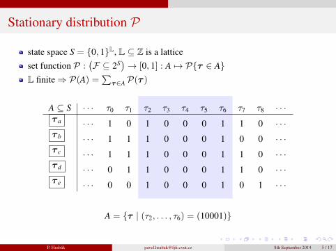
Stationary distribution P
state space S = {0, 1}L, L ⊆ Z is a latticeset function P :
(F ⊆ 2S
)→ [0, 1] : A 7→ P{τ ∈ A}
L finite⇒ P(A) =∑
τ∈A P(τ )
A ⊆ S · · · τ0 τ1 τ2 τ3 τ4 τ5 τ6 τ7 τ8 · · ·τ a · · · 1 0 1 0 0 0 1 1 0 · · ·τ b · · · 1 1 1 0 0 0 1 0 0 · · ·τ c · · · 1 1 1 0 0 0 1 1 0 · · ·τ d · · · 0 1 1 0 0 0 1 1 0 · · ·τ e · · · 0 0 1 0 0 0 1 0 1 · · ·
A = {τ | (τ2, . . . , τ6) = (10001)}
P. Hrabak [email protected] 8th September 2014 5 / 17

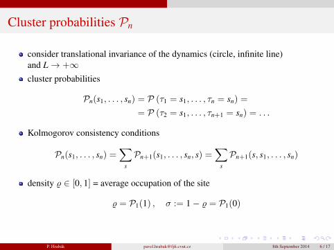
Cluster probabilities Pn
consider translational invariance of the dynamics (circle, infinite line)and L→ +∞
cluster probabilities
Pn(s1, . . . , sn) = P (τ1 = s1, . . . , τn = sn) =
= P (τ2 = s1, . . . , τn+1 = sn) = . . .
Kolmogorov consistency conditions
Pn(s1, . . . , sn) =∑
s
Pn+1(s1, . . . , sn, s) =∑
s
Pn+1(s, s1, . . . , sn)
density % ∈ [0, 1] = average occupation of the site
% = P1(1) , σ := 1− % = P1(0)
P. Hrabak [email protected] 8th September 2014 6 / 17

Cluster probabilities Pn
consider translational invariance of the dynamics (circle, infinite line)and L→ +∞cluster probabilities
Pn(s1, . . . , sn) = P (τ1 = s1, . . . , τn = sn) =
= P (τ2 = s1, . . . , τn+1 = sn) = . . .
Kolmogorov consistency conditions
Pn(s1, . . . , sn) =∑
s
Pn+1(s1, . . . , sn, s) =∑
s
Pn+1(s, s1, . . . , sn)
density % ∈ [0, 1] = average occupation of the site
% = P1(1) , σ := 1− % = P1(0)
P. Hrabak [email protected] 8th September 2014 6 / 17

Distance-headway and block-length distribution
distance-headway probability n ≥ 0 × × × ×
Pdh(n) = P(1
n︷ ︸︸ ︷00 . . . 0 1 | τ0 = 1
)=Pn+2
(1
n︷ ︸︸ ︷00 . . . 0 1
)P1(1)
block-length probability m ≥ 0 × ×
Qbl(m) = P(0
m︷ ︸︸ ︷11 . . . 1 0 | τ0 = 0
)=Pn+2
(0
m︷ ︸︸ ︷11 . . . 1 0
)P1(0)
P. Hrabak [email protected] 8th September 2014 7 / 17

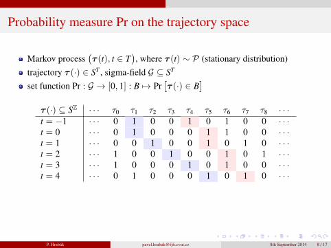
Probability measure Pr on the trajectory space
Markov process(τ (t), t ∈ T
), where τ (t) ∼ P (stationary distribution)
trajectory τ (·) ∈ ST , sigma-field G ⊆ ST
set function Pr : G → [0, 1] : B 7→ Pr[τ (·) ∈ B
]τ (·) ⊆ SZ · · · τ0 τ1 τ2 τ3 τ4 τ5 τ6 τ7 τ8 · · ·t = −1 · · · 0 1 0 0 1 0 1 0 0 · · ·t = 0 · · · 0 1 0 0 0 1 1 0 0 · · ·t = 1 · · · 0 0 1 0 0 1 0 1 0 · · ·t = 2 · · · 1 0 0 1 0 0 1 0 1 · · ·t = 3 · · · 1 0 0 0 1 0 1 0 0 · · ·t = 4 · · · 0 1 0 0 0 1 0 1 0 · · ·
B ={τ (·) | τ4
([−1, 0, 1, 2, 3, 4]
)= (1, 0, 0, 0, 1, 0)
}
P. Hrabak [email protected] 8th September 2014 8 / 17

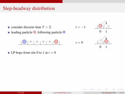
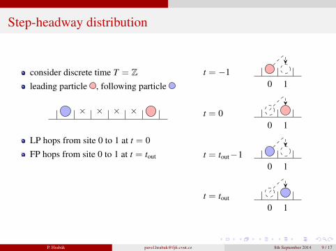
Step-headway distribution
consider discrete time T = Zleading particle , following particle
× × × ×
LP hops from site 0 to 1 at t = 0FP hops from site 0 to 1 at t = tout
step-headway probability
f (k) = Pr(tout = k | LP 0→ 1 at t = 0
)
t = −10 1
t = 00 1
t = tout−10 1
t = tout
0 1
P. Hrabak [email protected] 8th September 2014 9 / 17
Step-headway distribution
consider discrete time T = Zleading particle , following particle
× × × ×
LP hops from site 0 to 1 at t = 0
FP hops from site 0 to 1 at t = tout
step-headway probability
f (k) = Pr(tout = k | LP 0→ 1 at t = 0
)
t = −10 1
t = 00 1
t = tout−10 1
t = tout
0 1
P. Hrabak [email protected] 8th September 2014 9 / 17
Step-headway distribution
consider discrete time T = Zleading particle , following particle
× × × ×
LP hops from site 0 to 1 at t = 0FP hops from site 0 to 1 at t = tout
step-headway probability
f (k) = Pr(tout = k | LP 0→ 1 at t = 0
)
t = −10 1
t = 00 1
t = tout−10 1
t = tout
0 1
P. Hrabak [email protected] 8th September 2014 9 / 17
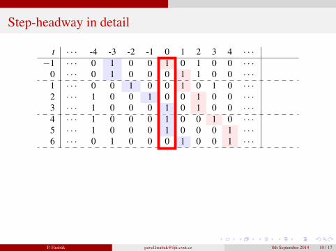
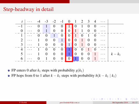
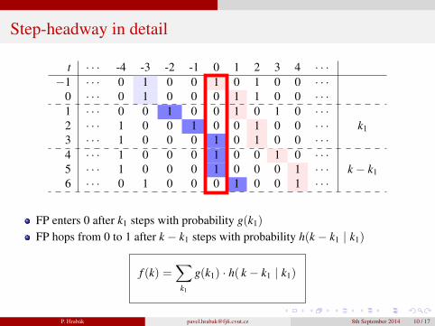
Step-headway in detail
t · · · -4 -3 -2 -1 0 1 2 3 4 · · ·−1 · · · 0 1 0 0 1 0 1 0 0 · · ·
0 · · · 0 1 0 0 0 1 1 0 0 · · ·1 · · · 0 0 1 0 0 1 0 1 0 · · ·
k1
2 · · · 1 0 0 1 0 0 1 0 0 · · ·3 · · · 1 0 0 0 1 0 1 0 0 · · ·4 · · · 1 0 0 0 1 0 0 1 0 · · ·
k − k1
5 · · · 1 0 0 0 1 0 0 0 1 · · ·6 · · · 0 1 0 0 0 1 0 0 1 · · ·
FP enters 0 after k1 steps with probability g(k1)
FP hops from 0 to 1 after k − k1 steps with probability h(k − k1 | k1)
f (k) =∑
k1
g(k1) · h( k − k1 | k1)
P. Hrabak [email protected] 8th September 2014 10 / 17

Step-headway in detail
t · · · -4 -3 -2 -1 0 1 2 3 4 · · ·−1 · · · 0 1 0 0 1 0 1 0 0 · · ·
0 · · · 0 1 0 0 0 1 1 0 0 · · ·1 · · · 0 0 1 0 0 1 0 1 0 · · ·
k12 · · · 1 0 0 1 0 0 1 0 0 · · ·3 · · · 1 0 0 0 1 0 1 0 0 · · ·4 · · · 1 0 0 0 1 0 0 1 0 · · ·
k − k1
5 · · · 1 0 0 0 1 0 0 0 1 · · ·6 · · · 0 1 0 0 0 1 0 0 1 · · ·
FP enters 0 after k1 steps with probability g(k1)
FP hops from 0 to 1 after k − k1 steps with probability h(k − k1 | k1)
f (k) =∑
k1
g(k1) · h( k − k1 | k1)
P. Hrabak [email protected] 8th September 2014 10 / 17
Step-headway in detail
t · · · -4 -3 -2 -1 0 1 2 3 4 · · ·−1 · · · 0 1 0 0 1 0 1 0 0 · · ·
0 · · · 0 1 0 0 0 1 1 0 0 · · ·1 · · · 0 0 1 0 0 1 0 1 0 · · ·
k1
2 · · · 1 0 0 1 0 0 1 0 0 · · ·3 · · · 1 0 0 0 1 0 1 0 0 · · ·4 · · · 1 0 0 0 1 0 0 1 0 · · ·
k − k15 · · · 1 0 0 0 1 0 0 0 1 · · ·6 · · · 0 1 0 0 0 1 0 0 1 · · ·
FP enters 0 after k1 steps with probability g(k1)
FP hops from 0 to 1 after k − k1 steps with probability h(k − k1 | k1)
f (k) =∑
k1
g(k1) · h( k − k1 | k1)
P. Hrabak [email protected] 8th September 2014 10 / 17
Step-headway in detail
t · · · -4 -3 -2 -1 0 1 2 3 4 · · ·−1 · · · 0 1 0 0 1 0 1 0 0 · · ·
0 · · · 0 1 0 0 0 1 1 0 0 · · ·1 · · · 0 0 1 0 0 1 0 1 0 · · ·
k12 · · · 1 0 0 1 0 0 1 0 0 · · ·3 · · · 1 0 0 0 1 0 1 0 0 · · ·4 · · · 1 0 0 0 1 0 0 1 0 · · ·
k − k15 · · · 1 0 0 0 1 0 0 0 1 · · ·6 · · · 0 1 0 0 0 1 0 0 1 · · ·
FP enters 0 after k1 steps with probability g(k1)
FP hops from 0 to 1 after k − k1 steps with probability h(k − k1 | k1)
f (k) =∑
k1
g(k1) · h( k − k1 | k1)
P. Hrabak [email protected] 8th September 2014 10 / 17

Step-headway in detail: g(k1)
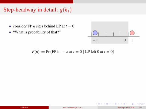
consider FP n sites behind LP at t = 0
“What is probability of that?”“Thank God, we are in stationary state!”
n-times
0 1−n
P(n) := Pr (FP in − n at t = 0 | LP left 0 at t = 0)
= P(1
n︷ ︸︸ ︷00 . . . 0 | τ0 = 0
)=Pn+1
(1
n︷ ︸︸ ︷00 . . . 0
)P1(0)
g(k1) =
+∞∑n=1
P(n) · Pr (k1 steps | FP in − n at t = 0 ∧ LP...)
P. Hrabak [email protected] 8th September 2014 11 / 17
Step-headway in detail: g(k1)
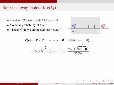
consider FP n sites behind LP at t = 0“What is probability of that?”
“Thank God, we are in stationary state!”
n-times
0 1−n
P(n) := Pr (FP in − n at t = 0 | LP left 0 at t = 0)
= P(1
n︷ ︸︸ ︷00 . . . 0 | τ0 = 0
)=Pn+1
(1
n︷ ︸︸ ︷00 . . . 0
)P1(0)
g(k1) =
+∞∑n=1
P(n) · Pr (k1 steps | FP in − n at t = 0 ∧ LP...)
P. Hrabak [email protected] 8th September 2014 11 / 17
Step-headway in detail: g(k1)
consider FP n sites behind LP at t = 0“What is probability of that?”“Thank God, we are in stationary state!”
n-times
0 1−n
P(n) := Pr (FP in − n at t = 0 | LP left 0 at t = 0)
= P(1
n︷ ︸︸ ︷00 . . . 0 | τ0 = 0
)=Pn+1
(1
n︷ ︸︸ ︷00 . . . 0
)P1(0)
g(k1) =
+∞∑n=1
P(n) · Pr (k1 steps | FP in − n at t = 0 ∧ LP...)
P. Hrabak [email protected] 8th September 2014 11 / 17
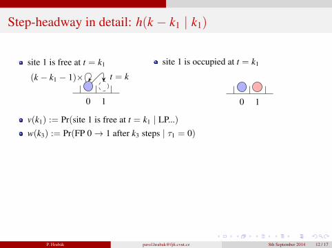
Step-headway in detail: h(k − k1 | k1)
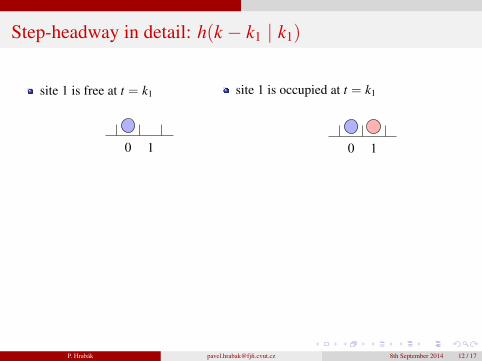
site 1 is free at t = k1
t = k(k − k1 − 1)×
0 1
site 1 is occupied at t = k1
t = k(k − k1 − k2 − 1)×(k2 − 1)× t = k1 + k2
0 1
v(k1) := Pr(site 1 is free at t = k1 | LP...)w(k3) := Pr(FP 0→ 1 after k3 steps | τ1 = 0)
u(k2) := Pr(LP 1→ 2 after k2 steps | LP in 1)
τ1, τ2, . . .in stationary
state ∀ t
h(k − k1 | k1) = v(k1)w(k − k1) + [1− v(k1)] ·k−k1∑k2=0
u(k2)w(k − k1 − k2)
P. Hrabak [email protected] 8th September 2014 12 / 17

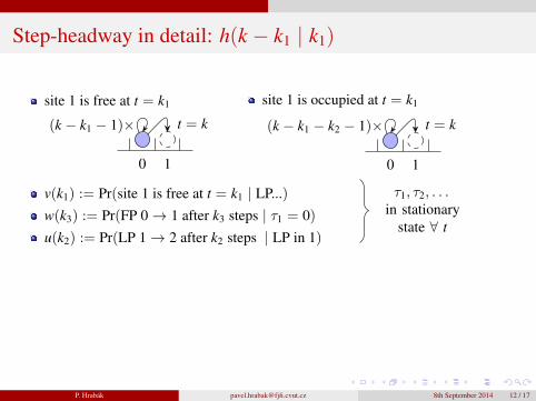
Step-headway in detail: h(k − k1 | k1)
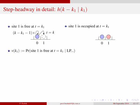
site 1 is free at t = k1
t = k(k − k1 − 1)×
0 1
site 1 is occupied at t = k1
t = k(k − k1 − k2 − 1)×(k2 − 1)× t = k1 + k2
0 1
v(k1) := Pr(site 1 is free at t = k1 | LP...)
w(k3) := Pr(FP 0→ 1 after k3 steps | τ1 = 0)
u(k2) := Pr(LP 1→ 2 after k2 steps | LP in 1)
τ1, τ2, . . .in stationary
state ∀ t
h(k − k1 | k1) = v(k1)w(k − k1) + [1− v(k1)] ·k−k1∑k2=0
u(k2)w(k − k1 − k2)
P. Hrabak [email protected] 8th September 2014 12 / 17

Step-headway in detail: h(k − k1 | k1)
site 1 is free at t = k1
t = k
(k − k1 − 1)×
0 1
site 1 is occupied at t = k1
t = k(k − k1 − k2 − 1)×(k2 − 1)× t = k1 + k2
0 1
v(k1) := Pr(site 1 is free at t = k1 | LP...)
w(k3) := Pr(FP 0→ 1 after k3 steps | τ1 = 0)
u(k2) := Pr(LP 1→ 2 after k2 steps | LP in 1)
τ1, τ2, . . .in stationary
state ∀ t
h(k − k1 | k1) = v(k1)w(k − k1) + [1− v(k1)] ·k−k1∑k2=0
u(k2)w(k − k1 − k2)
P. Hrabak [email protected] 8th September 2014 12 / 17
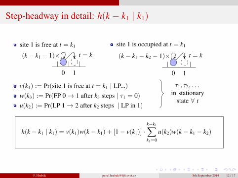
Step-headway in detail: h(k − k1 | k1)
site 1 is free at t = k1
t = k(k − k1 − 1)×
0 1
site 1 is occupied at t = k1
t = k(k − k1 − k2 − 1)×(k2 − 1)× t = k1 + k2
0 1
v(k1) := Pr(site 1 is free at t = k1 | LP...)
w(k3) := Pr(FP 0→ 1 after k3 steps | τ1 = 0)
u(k2) := Pr(LP 1→ 2 after k2 steps | LP in 1)
τ1, τ2, . . .in stationary
state ∀ t
h(k − k1 | k1) = v(k1)w(k − k1) + [1− v(k1)] ·k−k1∑k2=0
u(k2)w(k − k1 − k2)
P. Hrabak [email protected] 8th September 2014 12 / 17
Step-headway in detail: h(k − k1 | k1)
site 1 is free at t = k1
t = k(k − k1 − 1)×
0 1
site 1 is occupied at t = k1
t = k(k − k1 − k2 − 1)×(k2 − 1)× t = k1 + k2
0 1
v(k1) := Pr(site 1 is free at t = k1 | LP...)w(k3) := Pr(FP 0→ 1 after k3 steps | τ1 = 0)
u(k2) := Pr(LP 1→ 2 after k2 steps | LP in 1)
τ1, τ2, . . .in stationary
state ∀ t
h(k − k1 | k1) = v(k1)w(k − k1) + [1− v(k1)] ·k−k1∑k2=0
u(k2)w(k − k1 − k2)
P. Hrabak [email protected] 8th September 2014 12 / 17

Step-headway in detail: h(k − k1 | k1)
site 1 is free at t = k1
t = k(k − k1 − 1)×
0 1
site 1 is occupied at t = k1
t = k(k − k1 − k2 − 1)×
(k2 − 1)×
t = k1 + k2
0 1
v(k1) := Pr(site 1 is free at t = k1 | LP...)w(k3) := Pr(FP 0→ 1 after k3 steps | τ1 = 0)
u(k2) := Pr(LP 1→ 2 after k2 steps | LP in 1)
τ1, τ2, . . .in stationary
state ∀ t
h(k − k1 | k1) = v(k1)w(k − k1) + [1− v(k1)] ·k−k1∑k2=0
u(k2)w(k − k1 − k2)
P. Hrabak [email protected] 8th September 2014 12 / 17

Step-headway in detail: h(k − k1 | k1)
site 1 is free at t = k1
t = k(k − k1 − 1)×
0 1
site 1 is occupied at t = k1
t = k(k − k1 − k2 − 1)×
(k2 − 1)× t = k1 + k2
0 1
v(k1) := Pr(site 1 is free at t = k1 | LP...)w(k3) := Pr(FP 0→ 1 after k3 steps | τ1 = 0)
u(k2) := Pr(LP 1→ 2 after k2 steps | LP in 1)
τ1, τ2, . . .in stationary
state ∀ t
h(k − k1 | k1) = v(k1)w(k − k1) + [1− v(k1)] ·k−k1∑k2=0
u(k2)w(k − k1 − k2)
P. Hrabak [email protected] 8th September 2014 12 / 17
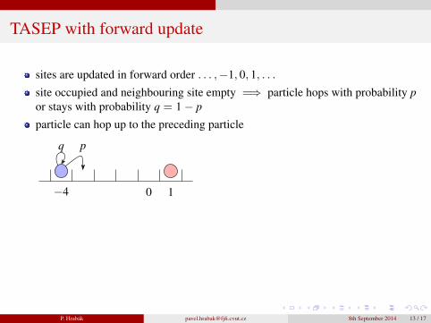
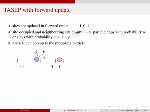
TASEP with forward update
sites are updated in forward order . . . ,−1, 0, 1, . . .site occupied and neighbouring site empty =⇒ particle hops with probability por stays with probability q = 1− p
particle can hop up to the preceding particle
pq
pq pq pq pq
0 1−4
q pq p2q p3q p4
0 1−4
p(x, x + n) = pnq , g(Nx,x+n) =
1 τx+j = 0 , j ≤ n ∧ τx+n+1 = 0 ,1/q τx+j = 0 , j ≤ n ∧ τx+n+1 = 1 ,0 otherwise
P. Hrabak [email protected] 8th September 2014 13 / 17

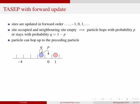
TASEP with forward update
sites are updated in forward order . . . ,−1, 0, 1, . . .site occupied and neighbouring site empty =⇒ particle hops with probability por stays with probability q = 1− p
particle can hop up to the preceding particle
pq
pq
pq pq pq
0 1−4
q pq p2q p3q p4
0 1−4
p(x, x + n) = pnq , g(Nx,x+n) =
1 τx+j = 0 , j ≤ n ∧ τx+n+1 = 0 ,1/q τx+j = 0 , j ≤ n ∧ τx+n+1 = 1 ,0 otherwise
P. Hrabak [email protected] 8th September 2014 13 / 17
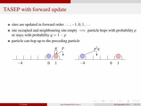
TASEP with forward update
sites are updated in forward order . . . ,−1, 0, 1, . . .site occupied and neighbouring site empty =⇒ particle hops with probability por stays with probability q = 1− p
particle can hop up to the preceding particle
pq pq
pq
pq pq
0 1−4
q pq p2q p3q p4
0 1−4
p(x, x + n) = pnq , g(Nx,x+n) =
1 τx+j = 0 , j ≤ n ∧ τx+n+1 = 0 ,1/q τx+j = 0 , j ≤ n ∧ τx+n+1 = 1 ,0 otherwise
P. Hrabak [email protected] 8th September 2014 13 / 17
TASEP with forward update
sites are updated in forward order . . . ,−1, 0, 1, . . .site occupied and neighbouring site empty =⇒ particle hops with probability por stays with probability q = 1− p
particle can hop up to the preceding particle
pq pq pq
pq
pq
0 1−4
q pq p2q p3q p4
0 1−4
p(x, x + n) = pnq , g(Nx,x+n) =
1 τx+j = 0 , j ≤ n ∧ τx+n+1 = 0 ,1/q τx+j = 0 , j ≤ n ∧ τx+n+1 = 1 ,0 otherwise
P. Hrabak [email protected] 8th September 2014 13 / 17

TASEP with forward update
sites are updated in forward order . . . ,−1, 0, 1, . . .site occupied and neighbouring site empty =⇒ particle hops with probability por stays with probability q = 1− p
particle can hop up to the preceding particle
pq pq pq pq
pq
0 1−4
q
pq p2q p3q p4
0 1−4
p(x, x + n) = pnq , g(Nx,x+n) =
1 τx+j = 0 , j ≤ n ∧ τx+n+1 = 0 ,1/q τx+j = 0 , j ≤ n ∧ τx+n+1 = 1 ,0 otherwise
P. Hrabak [email protected] 8th September 2014 13 / 17

TASEP with forward update
sites are updated in forward order . . . ,−1, 0, 1, . . .site occupied and neighbouring site empty =⇒ particle hops with probability por stays with probability q = 1− p
particle can hop up to the preceding particle
pq pq pq pq
pq
0 1−4
q
pq
p2q p3q p4
0 1−4
p(x, x + n) = pnq , g(Nx,x+n) =
1 τx+j = 0 , j ≤ n ∧ τx+n+1 = 0 ,1/q τx+j = 0 , j ≤ n ∧ τx+n+1 = 1 ,0 otherwise
P. Hrabak [email protected] 8th September 2014 13 / 17
TASEP with forward update
sites are updated in forward order . . . ,−1, 0, 1, . . .site occupied and neighbouring site empty =⇒ particle hops with probability por stays with probability q = 1− p
particle can hop up to the preceding particle
pq pq pq pq
pq
0 1−4
q pq
p2q
p3q p4
0 1−4
p(x, x + n) = pnq , g(Nx,x+n) =
1 τx+j = 0 , j ≤ n ∧ τx+n+1 = 0 ,1/q τx+j = 0 , j ≤ n ∧ τx+n+1 = 1 ,0 otherwise
P. Hrabak [email protected] 8th September 2014 13 / 17

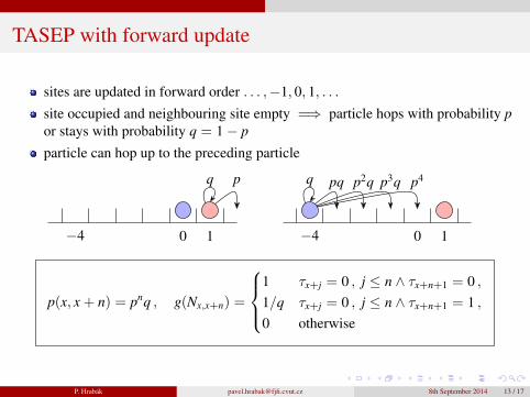
TASEP with forward update
sites are updated in forward order . . . ,−1, 0, 1, . . .site occupied and neighbouring site empty =⇒ particle hops with probability por stays with probability q = 1− p
particle can hop up to the preceding particle
pq pq pq pq
pq
0 1−4
q pq p2q
p3q
p4
0 1−4
p(x, x + n) = pnq , g(Nx,x+n) =
1 τx+j = 0 , j ≤ n ∧ τx+n+1 = 0 ,1/q τx+j = 0 , j ≤ n ∧ τx+n+1 = 1 ,0 otherwise
P. Hrabak [email protected] 8th September 2014 13 / 17

TASEP with forward update
sites are updated in forward order . . . ,−1, 0, 1, . . .site occupied and neighbouring site empty =⇒ particle hops with probability por stays with probability q = 1− p
particle can hop up to the preceding particle
pq pq pq pq
pq
0 1−4
q pq p2q p3q
p4
0 1−4
p(x, x + n) = pnq , g(Nx,x+n) =
1 τx+j = 0 , j ≤ n ∧ τx+n+1 = 0 ,1/q τx+j = 0 , j ≤ n ∧ τx+n+1 = 1 ,0 otherwise
P. Hrabak [email protected] 8th September 2014 13 / 17
TASEP with forward update
sites are updated in forward order . . . ,−1, 0, 1, . . .site occupied and neighbouring site empty =⇒ particle hops with probability por stays with probability q = 1− p
particle can hop up to the preceding particle
pq pq pq pq
pq
0 1−4
q pq p2q p3q p4
0 1−4
p(x, x + n) = pnq , g(Nx,x+n) =
1 τx+j = 0 , j ≤ n ∧ τx+n+1 = 0 ,1/q τx+j = 0 , j ≤ n ∧ τx+n+1 = 1 ,0 otherwise
P. Hrabak [email protected] 8th September 2014 13 / 17
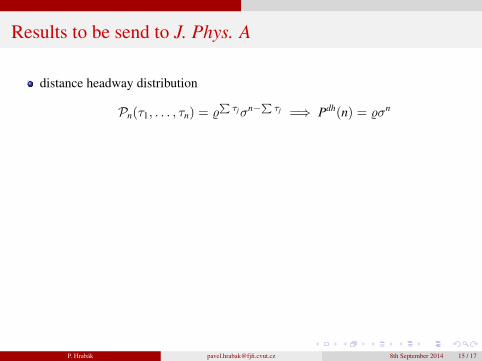
Results to be send to J. Phys. A
distance headway distribution
Pn(τ1, . . . , τn) = %∑τjσn−
∑τj =⇒ Pdh(n) = %σn
step-headway distribution
f→(k) = −p2kqk−1 +pσ%
[(1− pσ)k − qk]+
p%qσ
[(q
1− pσ
)k
− qk
]
time-headway distribution with p→ 0+ and t = p · k
f (t) =%
σ
(e−%t − e−t)+
σ
%
(e−σt − e−t)− te−t
P. Hrabak [email protected] 8th September 2014 15 / 17
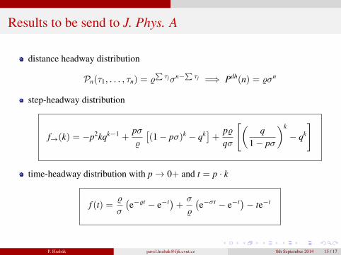

Comparison with the real-traffic data
normalization is necessary : t→ s, 〈∆s〉 = 1
τ(s) = 〈∆t〉f (t) , s = t/〈∆t〉 , 〈∆t〉 = 1/%σ .
τ(s) = 1σ2 e−s/σ + 1
%2 e−s/% −(
1σ2 + 1
%2
)e−s/σ% .
”particle-hole” symmetry %↔ 1− %
real traffic
0 0.5 1 1.5 2 2.5 3 3.5 40
0.2
0.4
0.6
0.8
1
1.2
1.4
time−headway s [normalized]
prob
abili
ty d
ensi
ty τ
(s)
ρ≈0
ρ=15 veh/km
ρ=40 veh/km
TASEP
0 0.5 1 1.5 2 2.5 3 3.5 40
0.2
0.4
0.6
0.8
1
time−headway s [normalized]
prob
abili
ty d
ensi
ty τ
(s)
ρ≈0
ρ=0.15 par/cell
ρ=0.5 par/cell
P. Hrabak [email protected] 8th September 2014 16 / 17


![Phytochromes and Phytochrome Interacting Factors1[OPEN] · Update on Phytochromes and Phytochrome Interacting Factors Phytochromes and Phytochrome Interacting Factors1[OPEN] Vinh](https://img.pdfslide.us/doc/110x75/5e9224c5cbd0a85457462c45/phytochromes-and-phytochrome-interacting-factors1open-update-on-phytochromes-and.jpg)


![On the concentration properties of Interacting …On the concentration properties of Interacting particle processes 4 85, 86], and the more recent article by R. Adamczak [1]. The best](https://img.pdfslide.us/doc/110x75/5f0265fe7e708231d40414af/on-the-concentration-properties-of-interacting-on-the-concentration-properties-of.jpg)


![[width=2cm]biipslogosmooth Biips software: …genome.jouy.inra.fr/applibugs/applibugs.14_11_28...SMC algorithm I A.k.a. interacting MCMC, particle filtering, sequential Monte Carlo](https://img.pdfslide.us/doc/110x75/5f0679b67e708231d4182dde/width2cmbiipslogosmooth-biips-software-smc-algorithm-i-aka-interacting.jpg)