University of Ljubljana

Faculty of computer and information science

Lina Lumburovska

Time-Efficient String Matching

Algorithms and the Brute-Force

Method

BACHELOR THESIS

UNIVERSITY STUDY PROGRAM

FIRST CYCLE

COMPUTER AND INFORMATION SCIENCE

Mentor: prof. dr. Borut Robic

Ljubljana, 2018

Univerza v Ljubljani

Fakulteta za racunalnistvo in informatiko

Lina Lumburovska

Casovno ucinkoviti algoritmi

ujemanja nizov in metoda grobe sile

DIPLOMSKO DELO

UNIVERZITETNI STUDIJSKI PROGRAM

PRVE STOPNJE

RACUNALNISTVO IN INFORMATIKA

Mentor: prof. dr. Borut Robic

Ljubljana, 2018

Copyright. The results of the bachelor thesis are the intellectual property

of the author and the Faculty of Computer and Information Science of the

University of Ljubljana. For the publication and use of the bachelor thesis,

the written consent of the author, the Faculty of Computer and Information

Science and the mentor is required.

Faculty of Computer and Information Science issues the following thesis:

Thesis subject:

Describe the main ideas, workings, computational complexity, and applica-

bility of modern algorithms for solving the string matching problem. De-

scribe their relation with the naive string matching based on the brute-force

method.

Fakulteta za racunalnistvo in informatiko izdaja naslednjo nalogo:

Tematika naloge:

Opisite osnovne zamisli, delovanje, racunsko zahtevnost in uporabnost sodob-

nih algoritmov za resevanje problema iskanja nizov. Opisite njihovo morebitno

povezavo z naivnim iskanjem nizov z metodo grobe sile.

Minimalna zahvala je majhen nacin, da izrazim izjemno hvaleznost in ljubezen

do moje druzine in vseh mojih prijateljev, ki so me podpirali ze od prvega

zacetka mojega akademskega potovanja. Nenazadnje bi se se posebej zah-

valila mojem mentorju, ki me je vodil pri sestavljanju te diplomske naloge v

odlicno delo.

Contents

Abstract

Povzetek

Daljsi povzetek

1 Introduction 1

2 Basic Concepts 3

2.1 Strings and Alphabets . . . . . . . . . . . . . . . . . . . . . . 3

2.2 String Concatenation and Kleene Closure . . . . . . . . . . . . 4

2.3 Substrings . . . . . . . . . . . . . . . . . . . . . . . . . . . . . 4

3 The String Matching Problem and its Algorithms 7

3.1 Definition of the Problem . . . . . . . . . . . . . . . . . . . . 8

3.2 Usage and Examples . . . . . . . . . . . . . . . . . . . . . . . 10

4 A Short History and the Most Known String Matching Al-

gorithms 13

4.1 Time Complexity . . . . . . . . . . . . . . . . . . . . . . . . . 15

4.2 Algorithms . . . . . . . . . . . . . . . . . . . . . . . . . . . . . 15

5 The Brute-Force (Naive) Algorithm 17

6 Knuth-Morris-Pratt Algorithm 21

6.1 KMP Algorithm with Finite Automation . . . . . . . . . . . . 24

7 Boyer-Moore Algorithm 27

8 Rabin-Karp Algorithm 33

9 Fast Hybrid Algorithm 39

9.1 Quick-Skip Search . . . . . . . . . . . . . . . . . . . . . . . . . 39

9.2 Tuned Boyer-Moore Algorithm . . . . . . . . . . . . . . . . . . 41

9.3 Definition of the Fast Hybrid Algorithm . . . . . . . . . . . . 41

10 Other Known Algorithms 43

10.1 Two-Way String Matching Algorithm . . . . . . . . . . . . . . 43

10.2 Backward Nondeterministic Dawg Matching Algorithm . . . . 44

10.3 Aho–Corasick Algorithm . . . . . . . . . . . . . . . . . . . . . 44

10.4 Commentz-Walter Algorithm . . . . . . . . . . . . . . . . . . 45

10.5 Horspool Algorithm . . . . . . . . . . . . . . . . . . . . . . . . 45

10.6 Raita Algorithm . . . . . . . . . . . . . . . . . . . . . . . . . . 45

10.7 Bitap Algorithm . . . . . . . . . . . . . . . . . . . . . . . . . . 46

11 Conclusion 47

Bibliography 47

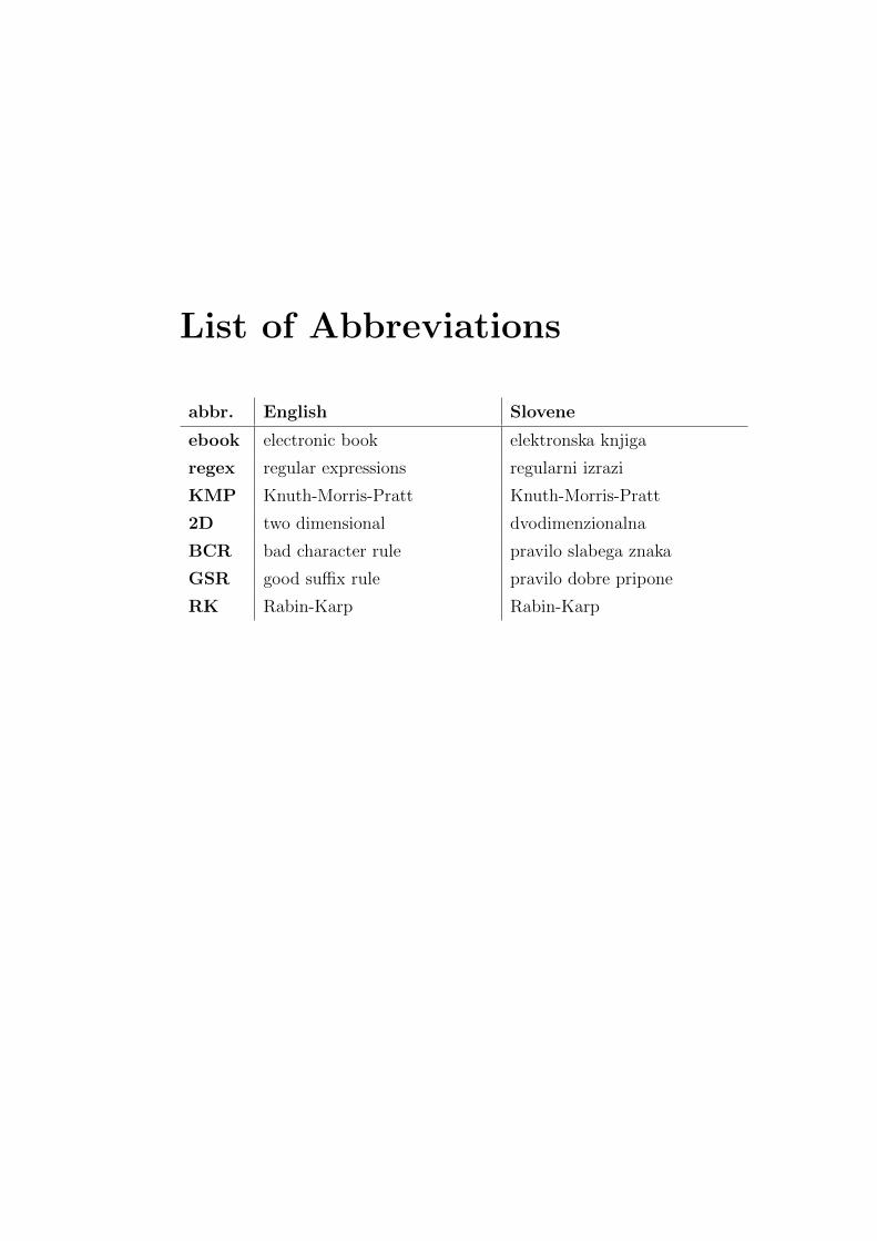
List of Abbreviations

abbr. English Slovene

ebook electronic book elektronska knjiga

regex regular expressions regularni izrazi

KMP Knuth-Morris-Pratt Knuth-Morris-Pratt

2D two dimensional dvodimenzionalna

BCR bad character rule pravilo slabega znaka

GSR good suffix rule pravilo dobre pripone

RK Rabin-Karp Rabin-Karp

Abstract

Title: Time-Efficient String Matching Algorithms and the Brute-Force Method

Author: Lina Lumburovska

One of the most researched areas of computer science is the string matching

problem. In everyday life, people read, write, and encounter character strings

all the time. Very often they want to find substrings (e.g. words) that match

parts of the original text and have higher probability of matching. Finding a

new efficient algorithm for the String Matching Problem involves a tremen-

dous number of testing, just to slightly improve on the existing algorithms.

In this, the algorithm based on the Brute-Force Method is of considerable

help, as many current algorithms are founded on it.

My bachelor thesis explores different algorithms for the String Matching

Problem and comes to a conclusion that each such algorithm has advan-

tages and disadvantages, and is suitable for solving a particular version of

the String Matching Problem and type of situations. Nevertheless, the most

used algorithm in practice is the Knuth-Morris-Pratt algorithm.

Keywords: string, matching, algorithm.

Povzetek

Naslov: Casovno ucinkoviti algoritmi ujemanja nizov in metoda grobe sile

Avtor: Lina Lumburovska

Eno izmed najbolj raziskanih podrocij na podrocju racunalnistva je problem

ujemanja nizov. V vsakodnevnem zivljenjem ljudje ves cas berejo, pisejo,

srecujejo nize in pogosto zelijo najti nekaj podnizov ali besed, ki se ujemajo

z izvirnim besedilom in imajo vecjo verjetnost ujemanja. Razvoj mnogih al-

goritmov za problem ujemanja nizov zahteva ogromno preizkusanja, ce zelimo

le malenkostno izboljsati kak obstojeci algoritem. Pri tem nam je velikokrat

v pomoc algoritem, ki deluje po metodi grobe sile, saj na njem temelji veliko

novejsih algoritmov.

V svoji diplomski nalogi sem raziskala razlicne vrste algoritmov za prob-

lem ujemanja nizov in prisla do zakljucka, da ima vsak tak algoritem svoje

prednosti in slabosti in je uporaben le za resevanje posebnih oblik tega prob-

lema in pripadajocih situacij. Vendar se v praksi izkaze, da je najpogosteje

uporabljen tako imenovani Knuth-Morris-Prattov algoritem.

Kljucne besede: niz, ujemanje, algoritem.

Daljsi povzetek

Naslov: Casovno ucinkoviti algoritmi ujemanja nizov in metoda grobe sile

Avtor: Lina Lumburovska

Na podrocju racunalnistva oziroma na podrocju algoritmov obstajajo razlicni

kriteriji za razdelitev algoritmov v skupine. Glavna delitev je narejena na

podlagi problemov in tezav, ki jih resuje vsak algoritem. Delitev izhaja iz

razlicni oblik resevanja problema, razlicne casovne in prostorske komplek-

snosti, drugacne kakovosti resitev, primernejsih primerov, ki jih resujejo, itd.

Ena izmed najbolj uporabnih skupin algoritmov je skupina algoritmov za

ujemanje nizov. To so algoritmi za iskanje podobnih ali enakih nizov znakov.

V praksi se najpogosteje uporabljajo za onemogocanje plagiatorstva. V svoji

diplomski nalogi bom opisala moderne algoritme za ujemanje nizov in ra-

zlozila, zakaj so boljsi od starejsih.

Problem ujemanja nizov imenujemo tudi problem iskanja nizov, saj v ra-

cunalnistvu poleg ujemanja danega vzorca iscemo tudi podnize, predpone,

pripone v dolgem besedilu. Problem torej ni le iskanje/ujemanja enega niza,

ampak tudi iskanje/ujemanje mnogih ali vseh. Kljub temu v vecini primerov

pojma iskanje in ujemanje uporabljamo kot sinonima.

Najpogosteje uporabljen algoritem je metoda grobe sile za iskanje podnizov,

ki jo pogosto imenujemo tudi naivni algoritem. Za skoraj vsak racunalniski

problem obstaja pripadajoca metoda grobe sile, ki pa obicajno ni najbolj

ucinkovita. V primeru iskanja in ujemanja nizov ta metoda preverja prav

vsak mozen polozaj vzorca znotraj besedila. To pomeni preverjanje vsakega

polozaja v besedilu, na katerem se vzorec lahko ujema. Ker ni nujno, da bo

do ujemanja prislo, algoritem vrne eno od dveh moznih logicnih vrednosti:

resnicno ali neresnicno. Ce obstaja ujemanje na dolocenem polozaju, vrne

metoda vrednost resnicno, sicer pa vrne neresnicno. Tak algoritem lahko

graficno predstavimo tudi kot drsenje vzorca nad besedilom. Z uporabo

take predstavitve lahko enostavno opazimo, nad kateri del besedila se vzorec

premakne in ali se ujema z ustreznimi znaki besedila. Zaradi njegovega pre-

prostega nacina delovanja naivni algoritem ne potrebuje predprocesiranja -

pred zacetkom algoritma ni treba nicesar pripraviti. Naivni algoritem pa ni

optimalen, zato njegove pomanjkljivosti resujejo novi, modernejsi algoritmi,

ki so predmet moje naloge.

Naslednji algoritem, ki sem ga raziskala, je Knuth-Morris-Prattov algoritem.

Osnovna ideja tega algoritma temelji na naslednji predpostavki: kadarkoli je

zaznano neujemanje (znak vzorca ne sovpada z znakom teksta), so nekateri

znaki v besedilu ze znani, saj so se pred neujemanjem ujemali z nekaterimi

vzorci ali nobenim od njih. To informacijo algoritem uporabi, da ne pon-

avlja preverjanja in s tem zmanjsa casovno zahtevnost. Razlika med naivnim

algoritmom in Knuth-Morris-Prattovim algoritmom je v tem, da se naivni

algoritem vedno vrne na zacetek in primerjanje zacne pri prvem indeksu, kar

pomeni, da se ne izogiba ponavljanju primerjanja. Knuth-Morris-Prattov al-

goritem je najbolj znan algoritem zaradi svoje linearne casovne zahtevnosti

tudi v najslabsem primeru.

Ucinkovit algoritem za ujemanje nizov, ki je tudi uporabljan v praksi, je

Boyer-Moorov algoritem. Na splosno deluje hitreje, ce je vzorec daljsi. Ta

znacilnost je na podrocju algoritmov izjemno redka. Razlog za to je, da

algoritem zacne preverjanje ujemanja nizov pri repu vzorca namesto pri nje-

govi glavi in preskakuje vzdolz besedila v skokih po vec znakov, namesto

da bi iskal vsak posamezni znak v besedilu. Eden od glavnih razlogov za

priljubljenost Boyer-Moorerovega algoritma je v njegovem predprocesiranju.

Algoritem je primeren za aplikacije, kjer je vzorec veliko krajsi od besedila.

To velja skoraj vedno, zato se algoritem pogosto uporablja v praksi pa tudi

teoriji.

Rabin in Karp sta odkrila popolnoma drugacen pristop k iskanju podni-

zov, ki uporablja zgoscevalne funkcije. Zgoscevalna funkcija je metoda, ki

se uporablja za preslikavanje podatkov poljubne velikosti v podatke fiksne

velikosti. Funkcija vrne vrednosti, ki so vcasih imenovane tudi vrednosti

zgoscevalne funkcije ali kar zgoscevalne vrednosti. Funkcije se pogosto za-

menjuje s pojmi kot so: prstni odtisi, kontrolne vsote, kontrolna stevila,

popravki napak ipd., kar poveca uporabljenost v praksi. Razlicni problemi

na splosno uporabljajo razlicne zgoscevalne funkcije. Za problem ujemanja

nizov je, taka funkcija zgrajena in namenjena podnizom.

V 21. stoletju, ko vsa tehnologija napreduje hitreje kot katero koli drugo

podrocje nasega zivljenja, se podrocje algoritmov vsak dan posodablja. Na-

jnovejsi algoritem za resavanje problema ujemanja nizov je pa pod imenom

hitri hibridni algoritem. Sestavljen je na osnovi dveh algoritmov: algoritma

s hitrim preskakovanjem in izboljsanega Boyer-Mooreovega algoritma. Hitri

hibridni algoritem je ucinkovit zaradi preskakovanja nepotrebnih preverjanj.

V povzetku sem omenila le najbolj znane algoritme, ceprav jih se nekaj.

Kadar so racunske viri (cas, prostor) omejeni, je pri resavanju problema

iskanja vzrocov zelo pomembno zmanjsanje casa in prostora, ki sta za to

potrebna. Mnogo sodobnih, t.j. novejsih algoritmov se v osnovi naslanja na

metodo grobe sile, a to metodo tako ali drugace izboljsajo.

Knuth-Morris-Prattov algoritem se v praksi izkaze kot najboljsi, na drugem

mestu pa mu sledi Boyer-Mooreov algoritem. Glede na izbrana merila, ome-

jene racunalniske vire in jasno definiran problem, vedno lahko dolocimo tis-

tega med znanimi algoritmi, ki bo najucinkovitejsi.

Kljucne besede: niz, ujemanje, algoritem.

Chapter 1

Introduction

In computer science, in the field of algorithms, there are different cri-

teria for dividing algorithms into groups. The main criterion is the kind of

computational problem to be solved. Besides this leading division, there is a

sub-division inside every group. This can be based on different kind of solu-

tions for the problem, different time and space complexities, different quality

of the solutions, more suitable examples they are solving etc.

One of the most useful groups of algorithms are the string matching

algorithms. Those are algorithms for searching similar or equal strings of

characters. Its dominant usage in practice is plagiarism. In my bachelor

thesis, I will describe highly sophisticated string matching algorithms and

explain/argue why they are better than the older ones.

Human communication [20] involves exchanging of strings of charac-

ters. Accordingly, numerous important and familiar applications are based

on processing of character strings. Below are listed some well-known practical

examples whose results are similar or equal strings:

• searching web pages that contain a given key word (Here, browser re-

turns a list of matches based on the key word);

• sending a text message, email or downloading an ebook (Here, trans-

mitting a string is transmitted from one to another place. This process

is called communication system and applications that process strings

1

2 Lina Lumburovska

for this purpose were an original for the development of string matching

algorithms. );

• translating a program (Here, translators such as compilers, interpreters

and assemblers convert programs from one form into another. Program-

ming systems use highly sophisticated string processing techniques,

where strings were used to construct formal written languages and al-

phabets.)

Chapter 2

Basic Concepts

2.1 Strings and Alphabets

A string [14, 18, 19, 20] is a sequence of characters, which is used as a

constant or variable of some type in programming languages. It is considered

as a data type and sometimes implemented as an array of bytes data struc-

ture. Each element of the array is in most of the cases a simple character.

Depending on the programming language, strings can be statically allocated

(with a fixed maximum length) or dynamically allocated (with variable num-

ber of characters).

An alphabet has a finite number of elements, called symbols, and can-

not be empty. Let Σ be an alphabet. A string (sometimes it is called word)

is a sequence of characters from Σ. For example, if Σ=0,1, a string is any

sequence of zeros and ones. Therefore, 01001 is a string over the alphabet

0,1. The number of all symbols in a given strings is called the length of

the string. The length of a string is a non-negative integer, and is denoted

by |s|. The empty string has zero elements and is usually denoted by ε.

3

4 Lina Lumburovska

2.2 String Concatenation and Kleene Closure

The string concatenation is the operation which joins two or more

strings into one string by attaching one string to the end of another string.

Here is a simple example: if u = tree and v = house, then the concatenated

string uv is the uv = treehouse. Also, the string housetree is a string concate-

nation of the same words, but in different order vu. Note that |uv| = |u|+|v|.The concatenation S1S2 of two sets of strings, S1 and S2, is another set of

strings and is defined by S1S2 = uv : u ∈ S1, v ∈ S2. Here, uv is concate-

nation of strings u and v.

The Kleene closure of an alphabet Σ is the set of all strings over Σ,

and it is denoted by Σ∗. Kleene closure of a set is a countably infinite set in

which each string has a finite length. Formally,

Σ∗ =⋃

n∈N∪0

Σn (2.1)

Due to the fact that Kleene closure never has zero elements, it contains only

an empty string if and only if the length of the alphabet is zero. For instance,

if Σ=0,1, then

Σ∗ = ε, 0, 1, 00, 01, 10, 11, 000, 001, 010, 011, 100, 101, 110, 111, 0000, 00001, ...A formal language over an alphabet is any subset of the Σ∗.

2.3 Substrings

A contiguous sequence of characters within a string is a substring

of that string [15, 18, 19, 20]. For example, the sequence the best of is a

substring of the string It was the best of me. But note that, Itwasme is a

subsequence of the same string, although not its substring. A substring T

is called a factor of a string T = t1 . . . tn if T= t1+i . . . tm+i, where 0 ≤ i

and m+ i ≤ n. Substrings are used as patterns in string searching or string

matching algorithms.

A string of length n > 0 has n(n+1)2

non-empty substrings.

Diplomska naloga 5

Often used terms when dealing with strings, substrings and string matching

algorithms are also the following:

• prefix: a prefix of a string T = t1 . . . tn is any string T =t1 . . . tm ,

where m ≤ n.

• suffix: a suffix of a string T = t1 . . . tn is any string T =tm . . . tn ,

where m ≤ n.

• rotation of a string: rotation of ε is ε, while rotation of au is ua,

where u is a string and a is a symbol.

• reverse of a string: reverse of a is a, while reverse of uv is reverse of

v concatenated with reverse of u (i.e. aR = a, (uv)R = vRuR).

The empty string ε is both prefix and suffix of every string.

For instance, the string x = abcca has a prefix w = ab and suffix y = cca

(x = wy). It is useful to note that for any strings x, y and any character a,

y is a suffix of x if and only if ya is a suffix of xa. Similarly for a prefix. This

leads to the conclusion that the relations, ”to be a prefix of” and ”to be a

suffix of” are transitive. This is proven by the following lemma.

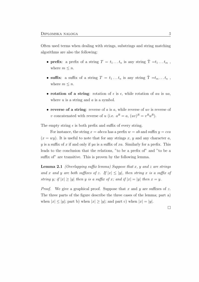
Lemma 2.1 (Overlapping suffix lemma) Suppose that x, y and z are strings

and x and y are both suffixes of z. If |x| ≤ |y|, then string x is a suffix of

string y; if |x| ≥ |y| then y is a suffix of x; and if |x| = |y| then x = y.

Proof. We give a graphical proof. Suppose that x and y are suffixes of z.

The three parts of the figure describe the three cases of the lemma; part a)

when |x| ≤ |y|; part b) when |x| ≥ |y|; and part c) when |x| = |y|.

6 Lina Lumburovska

Figure 2.1: Graphical proof of Lemma 2.1

Chapter 3

The String Matching Problem

and its Algorithms

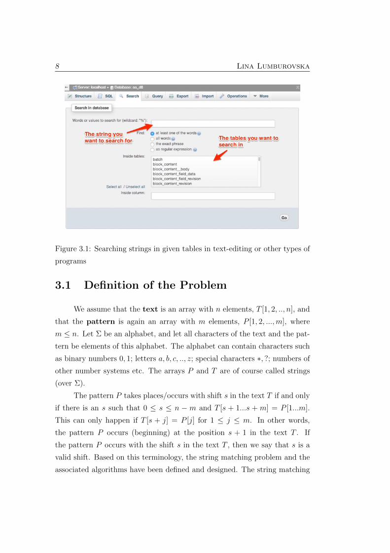
A frequently arising problem in text-editing programs is finding all oc-

currences of a pattern in a text. Typically, the text represents a document

being edited and the pattern is a word given by the user. Well-designed and

efficient algorithms for this problem can significantly improve the responsive-

ness of the text-editing programs.

As we will see, the string matching problem has been researched throughly

and there were many attempts during the history to find better algorithms

for this problem in terms of smaller time and space complexity.

7

8 Lina Lumburovska

Figure 3.1: Searching strings in given tables in text-editing or other types of

programs

3.1 Definition of the Problem

We assume that the text is an array with n elements, T [1, 2, .., n], and

that the pattern is again an array with m elements, P [1, 2, ...,m], where

m ≤ n. Let Σ be an alphabet, and let all characters of the text and the pat-

tern be elements of this alphabet. The alphabet can contain characters such

as binary numbers 0, 1; letters a, b, c, .., z; special characters ∗, ?; numbers of

other number systems etc. The arrays P and T are of course called strings

(over Σ).

The pattern P takes places/occurs with shift s in the text T if and only

if there is an s such that 0 ≤ s ≤ n − m and T [s + 1...s + m] = P [1...m].

This can only happen if T [s + j] = P [j] for 1 ≤ j ≤ m. In other words,

the pattern P occurs (beginning) at the position s + 1 in the text T . If

the pattern P occurs with the shift s in the text T , then we say that s is a

valid shift. Based on this terminology, the string matching problem and the

associated algorithms have been defined and designed. The string matching

Diplomska naloga 9

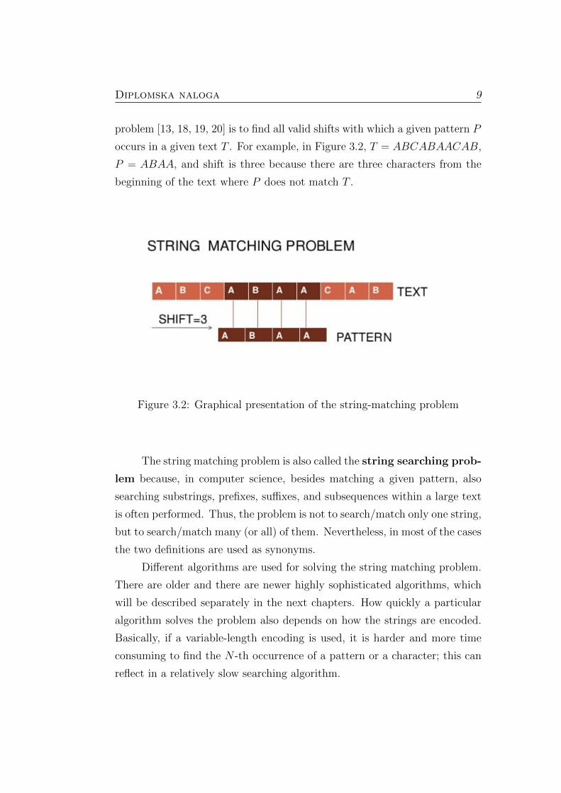
problem [13, 18, 19, 20] is to find all valid shifts with which a given pattern P

occurs in a given text T . For example, in Figure 3.2, T = ABCABAACAB,

P = ABAA, and shift is three because there are three characters from the

beginning of the text where P does not match T .

Figure 3.2: Graphical presentation of the string-matching problem

The string matching problem is also called the string searching prob-

lem because, in computer science, besides matching a given pattern, also

searching substrings, prefixes, suffixes, and subsequences within a large text

is often performed. Thus, the problem is not to search/match only one string,

but to search/match many (or all) of them. Nevertheless, in most of the cases

the two definitions are used as synonyms.

Different algorithms are used for solving the string matching problem.

There are older and there are newer highly sophisticated algorithms, which

will be described separately in the next chapters. How quickly a particular

algorithm solves the problem also depends on how the strings are encoded.

Basically, if a variable-length encoding is used, it is harder and more time

consuming to find the N -th occurrence of a pattern or a character; this can

reflect in a relatively slow searching algorithm.

10 Lina Lumburovska

3.2 Usage and Examples

Often a large text T is called the ”haystack”; in this case the pattern

P is called the ”needle”. For example, in the following sentence, by using a

pattern P equal to the word ”to”, the goal is to find several (or all) occur-

rences of the needle P within the haystack T . The text/sentence is T = ”To

be or not to be is a question that requires you to think”. Certain searches

might request the first occurrence of the needle, which is the first word in

the haystack. A different search might request all occurrences, which are

three. Yet another search might ask for the last occurrence of the needle in

the haystack, which is the second word from the end.

When a pattern contains more than one word, we often use a process

called normalization. In the above example, if we take the pattern ”to be”,

the normalization enables a string matching algorithm to succeed even if

there is something between ”to” and ”be”, such as:

• more than one space;

• line-breaks, tabs and non-breaking spaces;

• hyphen;

• tags, footnotes, list-numbers, embedded images, and so on.

String matching algorithms generally must succeed in all these cases.

Moreover, sometimes there are characters that should be treated as syn-

onymous. Such characters are usually used in the following systems/alphabets:

• In Latin-based alphabet, where it is expected that string matching al-

gorithms will ignore difference between lower-case and upper-case letter

(although in this system they are distinguished) ;

• Languages that contain ligatures, where one complex character contains

two or more simple characters joined together (e.g. æ);

Diplomska naloga 11

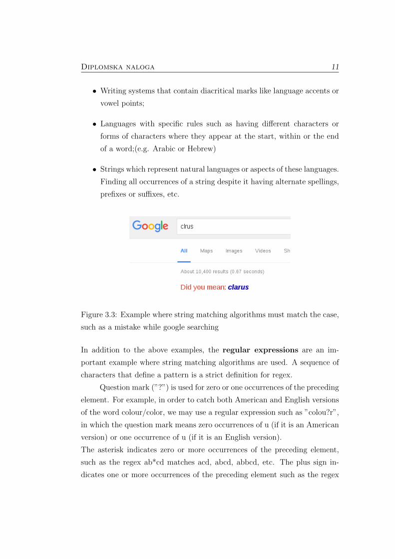
• Writing systems that contain diacritical marks like language accents or

vowel points;

• Languages with specific rules such as having different characters or

forms of characters where they appear at the start, within or the end

of a word;(e.g. Arabic or Hebrew)

• Strings which represent natural languages or aspects of these languages.

Finding all occurrences of a string despite it having alternate spellings,

prefixes or suffixes, etc.

Figure 3.3: Example where string matching algorithms must match the case,

such as a mistake while google searching

In addition to the above examples, the regular expressions are an im-

portant example where string matching algorithms are used. A sequence of

characters that define a pattern is a strict definition for regex.

Question mark (”?”) is used for zero or one occurrences of the preceding

element. For example, in order to catch both American and English versions

of the word colour/color, we may use a regular expression such as ”colou?r”,

in which the question mark means zero occurrences of u (if it is an American

version) or one occurrence of u (if it is an English version).

The asterisk indicates zero or more occurrences of the preceding element,

such as the regex ab*cd matches acd, abcd, abbcd, etc. The plus sign in-

dicates one or more occurrences of the preceding element such as the regex

12 Lina Lumburovska

ab+cd matches abcd or abbcd but compared with the asterisk it does not

match acd, because in it, the letter b has to appear at least once.

Chapter 4

A Short History and the Most

Known String Matching

Algorithms

String matching algorithms have an interesting history, which we here

summarize to help placing the various methods in the right perspective

[18, 19, 20].

The most frequently used algorithm for substring search has always

been the simple brute-force algorithm, which is also known as the naive

string searching algorithm. Almost every computational problem has a cor-

responding brute-force algorithm that solves it and usually this algorithm

is not the most efficient one. Interestingly, the brute-force string matching

algorithm is more or less efficient, except for the pathological cases where

the brute-force algorithm becomes too slow. Namely, in worst case scenarios,

the time complexity can rise to O(m*n) where m is pattern’s length and n

is text’s length. (The ”usual” running time is O(m+n), which is consider

less than O(m*n).) Furthermore, the brute-force string matching algorithm

is well-suited to standard architectural features of most computer systems,

so an optimized version of it can provide a standard benchmark, which is

almost unbreakable even with much more intelligent algorithm.

13

14 Lina Lumburovska

In 1970s, Stephen Cook published a theoretical solution for a specific

type of an abstract machine which implied the existence of an algorithm ca-

pable of solving the string-matching problem with worst-case time complex-

ity O(m+n). Donald Ervin Knuth and Vaughan Pratt laboriously followed

through the Cook’s construction, which was not intended to be practical.

They transformed Cook’s theorem into a relatively simple and practical al-

gorithm. The algorithm was a rare and satisfying example of a theoretical

result with an immediate practical applicability. Unexpectedly, it turned

out that James Hiran Morris had already discovered the same (equivalent)

algorithm as a solution to an annoying problem that arose when he was im-

plementing a text editor. The fact that the same algorithm is useful for

solving two different problems, indicated that there was something funda-

mental to this algorithm .

Knuth, Morris and Pratt did not publish their research on the algorithm

until 1976. In the meantime, two computer scientists, Robert S. Boyer and

Jeffrey S. Moore, constructed a string matching algorithm that was faster in

many applications, since it often examined only a fraction of the characters in

the text string. Due to this algorithm, many text editing programs achieved

noticeable speedups in substring search.

Eventually, it turned out that there are two different algorithms which

solve the same problem. Both Knuth-Morris-Pratt and Boyer-Moore algo-

rithm require additional time for preprocessing of the pattern. Unfortunately,

the preprocessing is hard to understand and has limited usefulness. In fact,

an unknown system programmer declared Morris’s algorithm too difficult to

understand and simply replaced it with the brute-force algorithm.

In 1980s, Michael O. Rabin and Richard M. Karp used hashing to solve

the string matching problem and developed an algorithm that is almost as

simple as the brute-force algorithm but has time complexity O(m+n). More-

over, their algorithm can be used for two-dimensional patterns and texts,

which makes it suitable for image processing.

Diplomska naloga 15

This is only a brief history with only the most significant events of

course. There have been many unsuccessful attempts. In the next section,

the most important string matching algorithms will be listed, and each of

them will be presented separately in the following chapters.

4.1 Time Complexity

During the history, several parameters had been researched in order to set

a criterium for determining the best algorithm for a given computational

problem . In the end, it turned out that the most useful and appropriate

criterium is the algorithm’s running time. In the filed of algorithms it

is known as the algorithm’s time complexity, i.e. the amount of time an

algorithm needs to process an instance of given computational problem.

We distinguish three cases of algorithm execution:

• best case (min. time needed for algorithm’s execution; notation: Ω)

• average case (average time needed for algorithm’s execution);

• worst case (max. time needed for algorithm’s execution; notation: O).

4.2 Algorithms

The most known algorithms for solving the string matching problem are:

• Brute-force algorithm (known as the naive algorithm),

• Knuth-Morris-Pratt algorithm,

• Boyer-Moore algorithm,

• Tuned Boyer-Moore algorithm,

• Rabin-Karp algorithm,

• Two-way string matching algorithm,

16 Lina Lumburovska

• String matching with finite automata,

• Quick-skip searching,

• Fast hybrid algorithm,

• Bitap algorithm (known as Baeza-Yates–Gonnet algorithm),

• BNDM (Backward Non-Deterministic Dawg Matching),

• Commentz-Walter algorithm,

• Aho–Corasick algorithm,

• Boyer–Moore–Horspool algorithm,

• Raita algorithm,

• BOM (Backward Oracle Matching),

• Apostolico–Giancarlo algorithm.

Chapter 5

The Brute-Force (Naive)

Algorithm

An obvious method [18, 19, 20] for searching and matching substrings

is to check every possible position of the pattern within the text. This means

checking each position in the text at which the pattern might match. How-

ever, it is not necessary that a position is matchable, so the algorithm returns

one of the two possible logical values: true or false. If there is a matching at

a position, it returns true; otherwise, it returns false.

In my bachelor thesis, I will use pseudocode. This is an informal high-

level description of the operating principle of an algorithm or computer pro-

gram. Pseudocodes provide the easiest way to describe a method even for

readers that have no knowledge of computer programming. Besides pseu-

docode, I will describe the most important algorithms in Java, one of the

most used programming languages. In such coses, I will present some func-

tions which already exist and describe how they are used.

Clearly, the naive algorithm for string matching accepts a pattern P

and a text T as two arguments. The pseudocode for the naive string match-

ing algorithm is presented below.

17

18 Lina Lumburovska

THE NAIVE STRING-MATCHING ALGORITHM (P,T)

m = length(P)

n = length(T)

for s = 0 to n-m

if P[1...,m] = T[s+1,...,s+m]

then print "The pattern occurs with shift" s

The variable m is the length of the pattern P and the variable n is the length

of the text T .

The naive algorithm only uses one loop that checks the condition

P [1, ...,M ] = T [s+ 1, .., s+M ] for each of the possible values of the shift s

which shows from which position the pattern matches the text.

The algorithm can also be graphically described as sliding the pattern

over the text. Using this, it can easily be seen at which shifts the pattern

matches the corresponding characters in the text. This is depicted in Figure

5.1, where the body of the for loop considers each possible shift explicitly.

The ”if condition” checks whether the current shift is valid or not, and per-

forms an implicit loop (which checks the characters of the pattern until either

all positions match or there is a mismatch). Each valid shift is printed out

by the last line (so there is an option to print more than one valid shift).

In the example presented in Figure 5.1, the pattern is P = aab and the

text is T = acaabc. The pattern is in each picture shifted by one character to

the right. Vertical lines in each picture connect the corresponding characters

that have been found to match. In contrast, jagged lines connect the first

mismatched character found, if any.

Diplomska naloga 19

Figure 5.1: Graphical presentation for the naive string matching algorithm

A simpler example using words from everyday life is given in Figure

5.2, where green color is used for matching characters and red for the mis-

matching ones. This example has only one occurrence of the pattern simple

in the text This is a simple example.

Figure 5.2: A simple example for only one occurrence of the pattern found

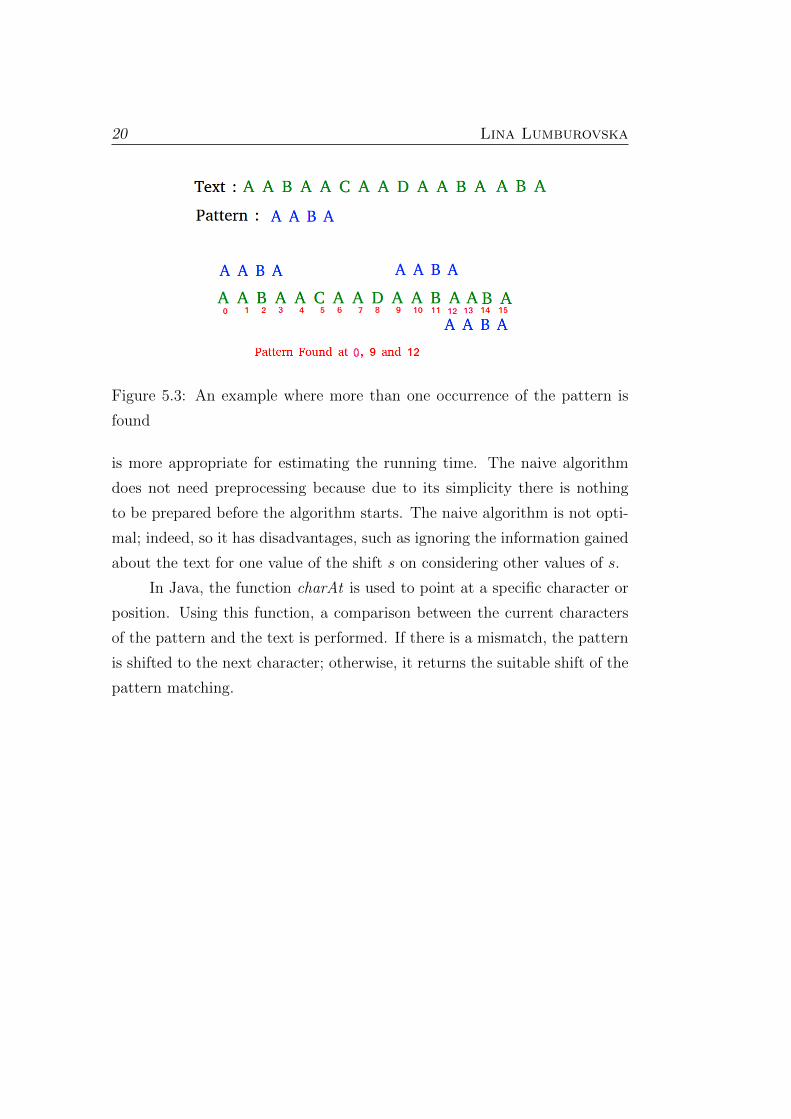
String matching algorithms are intended to find all occurrences of a

pattern. This is depicted in Figure 5.3, where the pattern AABA is found

three times in the given text.

The worst case input is when both, the pattern and the text have the

same form (for example, P = am and T = an), because it is necessary to

check m characters n −m + 1-times. This leads to the worst case running

time O((n-m+1)m), and this upper bound is tight. Fortunately, such sce-

narios hardly ever occurs. Most of the strings find a mismatch at the first

character of the pattern. That is why, in practice, the average running time

20 Lina Lumburovska

Figure 5.3: An example where more than one occurrence of the pattern is

found

is more appropriate for estimating the running time. The naive algorithm

does not need preprocessing because due to its simplicity there is nothing

to be prepared before the algorithm starts. The naive algorithm is not opti-

mal; indeed, so it has disadvantages, such as ignoring the information gained

about the text for one value of the shift s on considering other values of s.

In Java, the function charAt is used to point at a specific character or

position. Using this function, a comparison between the current characters

of the pattern and the text is performed. If there is a mismatch, the pattern

is shifted to the next character; otherwise, it returns the suitable shift of the

pattern matching.

Chapter 6

Knuth-Morris-Pratt Algorithm

The basic idea of this algorithm, discovered by Knuth, Morris and Pratt

[9, 8, 18, 19, 20], stems from the following assumption: whenever a mismatch

is detected, some of the characters in the text are already known, since they

matched some or none of the pattern characters prior to the mismatch. This

information is used as an advantage to avoid backing up the text pointer over

all those known characters.

Before presenting the pseudocode, we give an example. For observation

purposes we will allow the text to be T = ABAAAABAAAAAAAAA, the

searching pattern to be P = BAAAAAAAAA and the alphabet to have

only two characters, A and B. Suppose that there is a match on the first five

characters of the pattern and mismatch on the sixth one. When the mismatch

is detected, it is known that sixth character is not A but B. Text pointer is

now pointing at B. The key observation is that there is no need to back up the

text pointer i, since it is already known that the previous characters are As

and do not match the first character of the pattern. Knowing the information

about the currently pointed value, the index can be easily incremented by one

and compared to the next character of the pattern. The difference between

the brute-force algorithm and KMP is that the brute-force algorithm always

returns to the beginning and starts comparing from the first index. Since

KMP algorithm remembers the text pointer, there is no need to repeat it

21

22 Lina Lumburovska

all the time, and this results in a shorter running time and better time

complexity. The value of the text pointer i does not decrement and does not

change within the for loop and this method performs at most n character

comparisons.

It is important to note an exception when KMP algorithm does not

work properly. This is when the pattern could match itself at any position

overlapping the point of the mismatch. For example, when searching for the

pattern P = AABAAA in the text T = AABAABAAAA, first the mismatch

is detected on the fifth position, but there is a better restart at the third

position to continue the search, in order to miss the mismatch. The insight

of the KMP algorithm is that the user of the algorithm can decide ahead of

time exactly how to miss the mismatch and restart the search. Otherwise,

the algorithm will make an error and will not return the correct value.

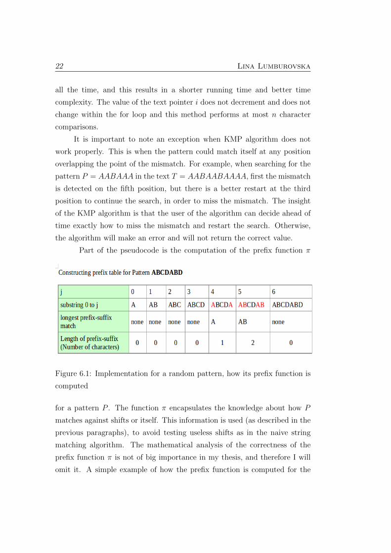
Part of the pseudocode is the computation of the prefix function π

Figure 6.1: Implementation for a random pattern, how its prefix function is

computed

for a pattern P . The function π encapsulates the knowledge about how P

matches against shifts or itself. This information is used (as described in the

previous paragraphs), to avoid testing useless shifts as in the naive string

matching algorithm. The mathematical analysis of the correctness of the

prefix function π is not of big importance in my thesis, and therefore I will

omit it. A simple example of how the prefix function is computed for the

Diplomska naloga 23

pattern P = ABCDABD is presented in Figure 6.1, where it is demonstrated

through six iterations how the longest prefix is determined and what is its

length.

To sum up, given a pattern P [1, . . . ,m], the prefix function for the

pattern P is the function π : 1, 2, . . . ,m = 0, 1, . . . ,m − 1 such that

π[q] = maxk : k ≤ q and Pk is a proper suffix of Pq. Informally, π[q] is the

length of the longest prefix of P which is Pk and q is the current character

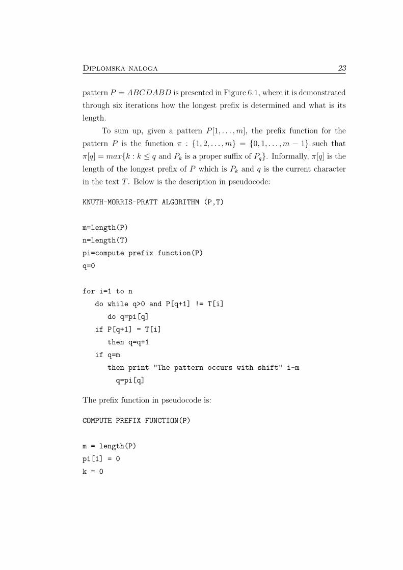
in the text T . Below is the description in pseudocode:

KNUTH-MORRIS-PRATT ALGORITHM (P,T)

m=length(P)

n=length(T)

pi=compute prefix function(P)

q=0

for i=1 to n

do while q>0 and P[q+1] != T[i]

do q=pi[q]

if P[q+1] = T[i]

then q=q+1

if q=m

then print "The pattern occurs with shift" i-m

q=pi[q]

The prefix function in pseudocode is:

COMPUTE PREFIX FUNCTION(P)

m = length(P)

pi[1] = 0

k = 0

24 Lina Lumburovska

for q = 2 to m

do while k > 0 and P[k+1] != P[q]

do k = pi[k]

if P[k+1] = P[q]

then k = k+1

pi[q] = k

return pi

By using this algorithm and the prefix function, the string matching

problem is solved in a way which gives better results than the naive algorithm.

The running time of the compute prefix function is Θ(m), which is determined

by the potential method of amortized analysis (such as using the value of k

to find the valuable information from mismatching). In order to determine

the running time of the whole algorithm, the same method is used (i.e. the

method of amortized analysis), but instead of k the value of q is applied in

the KMP-algorithm. This leads to a linear time complexity, Θ(n). The most

significant property of the KMP algorithm is that besides its average running

time also the worst case time is linear.

That makes KMP algorithm one of the highly sophisticated string matching

algorithms which are often used in practice.

6.1 KMP Algorithm with Finite Automation

A finite automation is used in the same way as an algorithm which,

given a pattern, must find the pattern in the text. A finite automation con-

sists of a starting state q0, a finite set of states Q, a set of accepting states A,

an input alphabet Σ, and a transition function δ that maps Q × Σ to Q. On

what follows, I will not be explaining finite automata; instead I will describe

the main idea of their use.

For each pattern P there exists an automation which must be con-

structed from the pattern in the preprocessing step. The automation is then

used to search the pattern in the text.

Diplomska naloga 25

To specify the string matching automation which corresponds to a given

pattern P [1, ..,m], we use an auxiliary function σ, called the suffix function.

This function maps from Σ∗ to 0,1,..,m so that σ(x) is the length of the

longest prefix of P that is a suffix of x:

σ(x) = max k : Pk is a suffix of x

The fact that the empty string ε is a suffix of every string makes the function

σ well-defined: for a pattern P with length m, we have σ(x)=m if and only

if P is a suffix of x.

It follows from the definition of the function σ that if x is a suffix of y, then

σ(x)≤ σ(y). Based on this, the string matching automation that corresponds

to a given pattern P can be constructed .

The scalability and importance of the suffix function within this topic is seen

from the following lemma.

Lemma 6.1 (Suffix function inequality lemma) For any string x and char-

acter a, the following holds σ(xa) ≤ σ(x) + 1.

Proof. Let variable r = σ(xa). If r = 0, then the conclusion σ(xa) ≤ σ(x) +

1 is trivially satisfied, by the nonnegativity of σ(x). So, assume that r ≥ 1.

Now Pr (P is a pattern) is a suffix of xa, by the definition of σ. Thus, Pr−1

is a suffix of x, by dropping the a from the end of Pr and from the end of xa.

Therefore, r − 1 ≤ σ(x), since σ(x) is the largest k, such that Pk is a suffix

of x and σ(xa) ≤ σ(x) + 1.

The pseudocode which clarifies the operation of the string matching

automation, represented by δ, is given below. The psedocode does exactly

the same as the ordinary KMP algorithm, i.e. finds occurrences of a given

pattern within a given text T .

26 Lina Lumburovska

KNUTH-MORRIS-PRATT AUTOMATION (T,delta, m)

n = length(T)

q = 0

for i = 1 to n

do q = delta(q, T[i])

if q=m

then print "Suitable pattern occurs with shift" i-m

In this type of substring searching, usually the preprocessing time is

not included. In other words, only the matching time is computed and it is

Θ(n).

Chapter 7

Boyer-Moore Algorithm

An efficient string matching algorithm that is the standard benchmark

for practical string-search literature is the Boyer-Moore algorithm [4, 18, 19,

20]. The algorithm is mainly used in computer science. In general, it runs

faster if the pattern is longer - a feature that is extremely rare in the field

of algorithms. The reason for that is that the algorithm seems to match on

the tail of the pattern rather than the head, and to skip along the text in

jumps of multiple characters rather than searching every single character in

the text.

A significantly faster string searching method is to scan the pattern

from right to left when trying to match it against the text. This can be

easily seen on the example, where P = BAABBAA, assuming there are

matches on the sixth and seventh character, but not on the fifth. Notice that

the pattern can be immediately slided seven positions to the right and can

move on checking the fourteenth character in the text. This can be done

because the partial match XAA, where X is not equal to B, does not appear

elsewhere in the pattern. The pattern could appear somewhere in the text

later, so there is a need to remember the position to restart the searching

method if there is a need.

Another example of Boyer-Moore shifting and searching, is shown in

Figure 7.1 where the text (or often called ”haystack”) is

27

28 Lina Lumburovska

T = FINDINAHAY STACKNEEDLE and the ”needle” (or the pattern)

is P = NEEDLE. The comparison starts from the rightmost character E

and it is compared with character N on the fifth position in the text. Since

N appears in the pattern, the pattern is slided five positions to the right to

line up the N in the text with the rightmost N in the pattern. The next

comparison is made with the rightmost E in the pattern with the character

S on the tenth position in the text. The difference with the mismatched S is

because S does not appear in the pattern so the pattern is slided six positions

to the right. The rightmost E in the pattern is matched with the character

on position 16, where a mismatch exists. N at position 15 is discovered and

the pattern is slid four positions. Finally, moving from right to left in the

text at position 20, the searched pattern is discovered within the text. The

algorithm uses only four comparisons to find the suitable pattern, which is

much better than with the naive algorithm.

One of the main reasons for the popularity of the Boyer-Moore algo-

Figure 7.1: Simple example for Boyer-Moore algorithm

rithm is in its preprocessing. The algorithm is suitable for applications when

the pattern is much shorter than the text. The condition is basically fulfilled

in almost every searching case, which is why the algorithm often is so used

in practice and theory.

There are two variants to perform shifting and preprocessing based on rules

called: the Bad Character Rule (BCR) and the Good Suffix Rule (GSR).

Diplomska naloga 29

Each rule has its own advantages and disadvantages, so their names ”good”

and ”bad”, do not mean that the one is actually better than the other.

• The Bad Character Rule (BCR)

Definition 7.0.1 This rule reviews the character in the text T where

comparison failed. When the next occurrence of the character to the left

is found in the pattern P, then a shift that brings that occurrence in line

with the mismatched occurrence in T is proposed. If the mismatched

character does not occur to the left in P, a new shift is proposed that

moves entire P past the point of mismatch.

Figure 7.2: Example of BCR, where b is a mismatched character. Skip

alignments until (a) b matches its opposite in P or (b) P moves past b.

To estimate BCR’s time complexity, we can use a 2D array where

the first dimension is indexed by the index of the character c in the

alphabet, and the second dimension is indexed by the index i from the

pattern. BCR will return the occurrence c of P with the index j < i

(or -1 if there is a mismatch). The time complexity of BCR is thus

O(1), a constant, which is in practice the best amount the searching

algorithms can have. The space complexity of BCR is O(k*n), where

k is the size (the number of characters) of the alphabet.

30 Lina Lumburovska

• The Good Suffix Rule (GSR)

This rule is the advantage of the Boyer-Moore algorithm, searching

from right to left.

Definition 7.0.2 Suppose that for a given alignment of P and T, a

substring t of T matches a suffix of P, but a mismatch occurs at the

next comparison to the left. Then find, if it exists, the rightmost copy

t’ of t in P such that t’ is not a suffix of P and the character to the left

of t’ in P differs from the character to the left of t in P. Shift P to the

right so that substring t’ in P aligns with substring t in T. If t’ does

not exist, then shift the left end of P past the left end of t in T by the

least amount so that a prefix of the shifted pattern matches a suffix of

t in T. If no such shift is possible, then shift P by x (x is the length of

the suffix) places to the right. If an occurrence of P is found, then shift

P by the least amount so that a proper prefix of the shifted P matches

a suffix of the occurrence of P in T. If no such shift is possible, then

shift P by x places, that is, shift P past t.

Figure 7.3: Example for GSR, where t is a substring of T and matches a

suffix of P. Skip alignments until t matches the opposite character in P (a),

a prefix of P matches a suffix of t (b) or P moves past the first matching

substring t(c).

Diplomska naloga 31

To determine GSR’s time complexity of the processing, we need two

arrays: L for the general case, and H for either when the general returns

a meaningless result or a match occurs.

It is known that for each i in L, the index i is the largest position less

than n and it is proven that the pattern P [i, ..., n] matches a suffix

P [1, ..., L[i]] and it is not equal to P [i − 1]. If this condition is not

satisfied, current index in the array is equal to zero. The index in H

is determined as the length of the largest suffix in P , which is at the

same time a prefix of P .

All of this leads to a linear time and space complexity, O(n), where n

is the length of the text.

To sum up, the algorithm’s time complexity is O(n+m), if and only if the

pattern does not appear in the text. However, this is not the best case sce-

nario, because the main aim of this algorithm is to find an existing substring

in the text. The worst case time complexity when the substring does appear

in the text is O(n*m). Although this is the same time complexity as the

time complexity of the naive algorithm, Boyer-Moore algorithm is in prac-

tice better due to its searching from tail to head, preprocessing, omitting

unnecessary comparisons, etc.

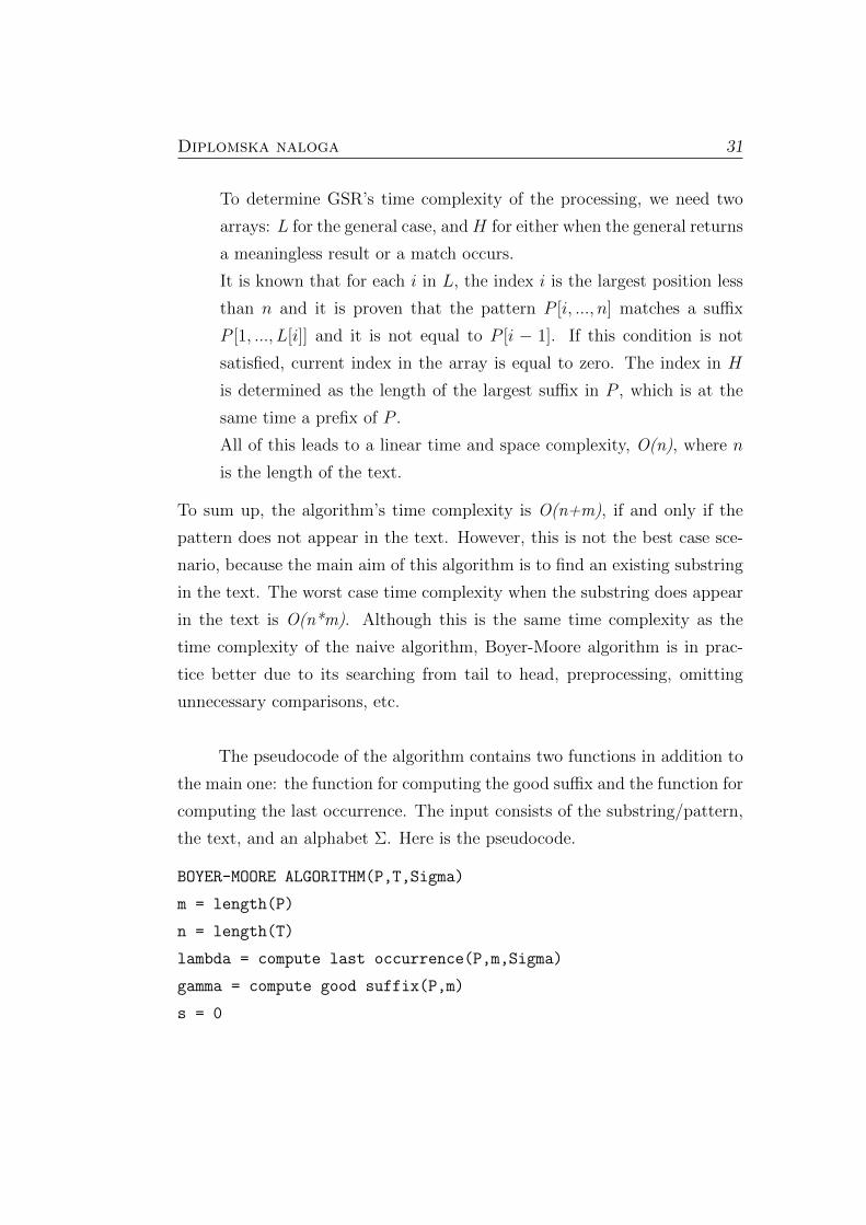
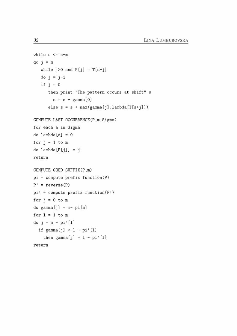
The pseudocode of the algorithm contains two functions in addition to

the main one: the function for computing the good suffix and the function for

computing the last occurrence. The input consists of the substring/pattern,

the text, and an alphabet Σ. Here is the pseudocode.

BOYER-MOORE ALGORITHM(P,T,Sigma)

m = length(P)

n = length(T)

lambda = compute last occurrence(P,m,Sigma)

gamma = compute good suffix(P,m)

s = 0

32 Lina Lumburovska

while s <= n-m

do j = m

while j>0 and P[j] = T[s+j]

do j = j-1

if j = 0

then print "The pattern occurs at shift" s

s = s + gamma[0]

else s = s + max(gamma[j],lambda[T[s+j]])

COMPUTE LAST OCCURRENCE(P,m,Sigma)

for each a in Sigma

do lambda[a] = 0

for j = 1 to m

do lambda[P[j]] = j

return

COMPUTE GOOD SUFFIX(P,m)

pi = compute prefix function(P)

P’ = reverse(P)

pi’ = compute prefix function(P’)

for j = 0 to m

do gamma[j] = m- pi[m]

for l = 1 to m

do j = m - pi’[l]

if gamma[j] > l - pi’[l]

then gamma[j] = l - pi’[l]

return

Chapter 8

Rabin-Karp Algorithm

A completely different approach to substring search which uses hash-

ing was discovered by Rabin and Karp [11, 18, 19, 20]. Hashing is a method

where a function, called the hash function, is used to map data of arbi-

trary size to data of a fixed size. The hash function returns values which

are sometimes named as hash values, hash codes, digests, or simply hashes.

(Hash functions are often confused with fingerprints, checksums, check dig-

its, error-correction etc.; and that is why this algorithm is also known as the

”Rabin-Karp fingerprint algorithm”.)

Different problems use, in general, different hashing methods (func-

tions). For the string matching problem, a hash function is constructed for

the pattern. The same hash function is used for finding a match for each

possible text substring of length m. The searching process is exactly the

same as if the pattern is stored in a hash table and then it performs a search

for each substring of the text. The main advantage (which has an impact on

the space complexity) is that there is no need to allocate the memory for the

hash table.

This process leads to a worse time complexity than the brute-force

algorithm. This is due to computing the hash function which involves all

characters and is more time-consuming since it only compares characters as

in the naive algorithm. In spite of that, in the real world it has been shown

33

34 Lina Lumburovska

that computing hash functions for m characters by Rabin-Karp’s algorithm

can be done in constant time and leads to a linear time substring matching

in practical situations. Hash functions are the reason why this algorithm

is in the group of effective string searching algorithm and has practical and

theoretical usage in many cases.

A string of length m corresponds to an m-digit base-R number. For

keys of this type, it is necessary to have a certain hash function which con-

verts an m-digit base-R to an integer value from 0 to Q−1. Modular hashing

is used in more complex cases, where this process takes the remainder of di-

viding the number with Q. Instead of the remainder in practice is mostly

used a random prime number Q, which is chosen in that way so the number

is as large as it is possible. In such cases, it is important to avoid overflow.

We give a simple example to demonstrate algorithm’s working. In this

example a small Q = 997 (a hash table size) is being used, which in real

situations hardly ever happens and R = 10. The pattern P = 26535 is

searched in the text T = 3141592653589793. The hash value for the pattern

is 26535%997 = 613, which means that iterations will be performed in the

text until there is found a substring with the same value (613) and has as

many characters as the pattern. In the example the substring is found in the

seventh iteration (the index is six) because the first six values returned are:

508, 201, 715, 971, 442 and 929. This is presented in Figures 8.1 and 8.2.

Figure 8.1: Simple example for computing a hash value for the pattern using

RK algorithm.

In the example, the number of the characters in the pattern is five and

still there is no problem. Difficulties appear when the number of the char-

acters is 100, 1000 etc. To handle such cases we often use the well-known

Horner’s method. This method is often used to calculate values of polynomi-

Diplomska naloga 35

Figure 8.2: Simple example for matching a pattern inside the text using RK

algorithm and hash values.

als. In Rabin-Karp algorithm only a simple application of Horner’s method is

used, in an elementary function which implements the hash function. There

is only one ”for loop”, which runs over all characters of the pattern (m times)

and computes the hash function by the formula given in the pseudocode be-

low.

HASH FUNCTION(key, m)

for j = 0 to m

h = (R * h + key[j]) % Q

return h

Because this algorithm uses some arithmetics, one more time the accent

will be on the Horner’s rule. The finite alphabet Σ has ten elements, i.e. ten

digits. Given a pattern P [1, ...,m], let p denote its corresponding decimal

value. Similarly, for a given text T [1, ..., n], let ts denote the decimal value of

the length-m substring T [s + 1, ..., s + m], for s = 0, 1, ..., n−m. Certainly,

ts = p if and only if T [s + 1, ..., s + m] = P [1, ...,m]; thus s is a valid shift

(and vise versa applies). If p can be somehow computed in time Θ(m) and

all the ts (for s = 0, 1, . . . ,m) values can be computed in time Θ(n−m+ 1),

then all valid shifts can be determined in time Θ(m) + Θ(n−m+ 1) which

36 Lina Lumburovska

is Θ(n).

By using Horner’s rule, p can be computed in time Θ(m):

p = P [m] + 10(P [m− 1] + 10(P [m− 2] + ...+ 10(P [2] + P [1])...)) (8.1)

Each of the other values t1, t2, ..., tn−m, can be computed in time Θ(n−m). Notice that ts+1 can be computed from ts in constant time, since:

ts+1 = 10(ts − 10m−1T [s+ 1]) + T [s+m+ 1] (8.2)

For example, let m = 5, q = 13, and T = [3, 1, 4, 1, 5, 2]. Consequently,

t0 = 31415. So,

t1 = 10(31415− 105−1 ∗ T [1]) + T [5 + 1] =

= 10(31415− 104 ∗ 3) + 2

= 10(1415) + 2

= 14152

This example shows how Horner’s rule is used: subtracting 10m−1 ∗T [s + 1] removes the high-order digit from ts; multiplying the result by 10

shifts the number left one position; and adding T [s + m + 1] brings in the

appropriate low-order digit.

The pseudocode for the RK algorithm accepts the text T , the searching

pattern P , Q and d, where d is basically |Σ| and is presented in the code

below. The function power(d,m-1) represents to dm−1 and mod is the usual

modulo function.

RABIN-KARP ALGORITHM(T,P,d,Q)

n = length(T)

m = length(P)

h = power(d, m-1) * mod Q

p = 0

t0 = 0

Diplomska naloga 37

for i = 1 to m

do p = (d * p + P[i]) * mod Q

t0 = (d * t0 + T[i]) * mod Q

for s = 0 to n - m

do if p = tS

then if P[1,..,m] = T[s+1,..,s+m]

then print "Suitable pattern occurs at shift" s

if s < n - m

then tS+1 = (d(tS - T[s+1]*h) + T[s+m+1]) * mod Q

The first for loop is used for preprocessing and takes Θ(m) time for the

first process. The second for loop is used for matching and takes Θ((n−m+

1)m) time in the worst case. If P = am and T = an, then the verifications

take time Θ((n−m+ 1)m), since each possible verification is a valid shift.

In some applications, not all verifications are valid shifts. Here, the

matching time of the Rabin-Karp algorithm is O((n-m+1) + cm) = O(n+m),

where c is a constant and does not have an impact on the matching time of

the algorithm. Since it is usually assumed that the length of the pattern is

smaller or at most equal, but never larger that the length of the text i.e.

m ≤ n, the matching time of the RK algorithm is O(n).

38 Lina Lumburovska

Chapter 9

Fast Hybrid Algorithm

As we are living in the twenty-first century, where all the technology

is moving forward faster than any other field in our everyday life, the field

of algorithms is getting new updates every day. The newest algorithm for

solving the string matching problem, found out the most recently, is based

on the Quick-skip and Tuned Boyer-Moore algorithm and is known as the

fast hybrid algorithm for string matching. Before explaining the main idea

of the fast hybrid algorithm, in the following subsections, I will describe the

two algorithms which fast hybrid algorithm is based on.

9.1 Quick-Skip Search

This algorithm [10] is a combination for solving two problems: the

Quick Search and the Skip Search. Similarly as in the other algorithms, there

are two phases in this algorithm: preprocessing and searching/matching. The

characters are preprocessed in the preprocessing phase and the information

obtained is used in the other phase to find the number of the comparisons

and all the attempts as well.

There are two different techniques involved in the preprocessing: the

first constructs the Quick Search bad character table (qsBc) and the second

constructs Skip Search buckets. Both techniques are used together, because

39

40 Lina Lumburovska

the first one, the table, contains the rightmost location for each alphabet in

the pattern, while the second one contains the leftmost location for all char-

acters in the pattern. The information gained in the preprocessing phase is

used in the matching phase to reduce the total number of comparisons and

the number of all (successful and unsuccessful) attempts. Both phases go

together, hand-in-hand, to improve efficiency of the algorithm by calculating

larger shift values.

The searching method consists of a four stages.

In the first stage, the algorithm finds the starting point S with a position

Tj within the text. The character of this certain position is aligned with the

suitable position of this character in the bucket. Even if there is a mismatch,

the algorithm continues shifting the pattern to the next character in the text

and avoiding mismatches, which definitely speeds up the algorithm.The al-

gorithm becomes faster because it avoids aligning the leftmost character of

the pattern and the window at the beginning of the searching phase.

In the second stage, the comparisons between the characters of the pattern

and the window are executed. These comparisons start from the leftmost

character of the pattern with the suitable position of the same character in

the window. This stage is only intended for accomplishing number of com-

parisons, and whether there is a match or mismatch is done in the next stage.

In the third stage, the algorithm calculates the shift value of the Skip Search

which is calculated differently depending on two situations, whether the char-

acter in the pattern occurs or does not occur in the last position of the bucket.

If it does, the shift value is calculated

skip shift = m + the current position of Tj (from the bucket) – the next

position of T

If it does not occur the shift value is calculated by subtracting the next

position value from the current position value of this character in the bucket.

The Quick Search shift value for this algorithm is assigned for a character

immediately next to the window.

In the last stage, the algorithm depends on the Quick Search shift. It is given

Diplomska naloga 41

in the pseudocode below using words, as it happens in different situations.

QUICK-SKIP SEACH(P,T)

m = length(P)

n = length(T)

if (Quick Shift > Skip Shift) and (Quick Search Shift < = m)

then Current Position of Tj = Position Next to the Window

if (Quick Shift > Skip Shift) and (Quick Search Shift > m)

then Current Position of Tj = Position Next to the Window + m

The algorithm has a worst running time Θ(n ∗m) and the best running time

is O(n/m).

9.2 Tuned Boyer-Moore Algorithm

Besides the algorithm explained in the previous section, the Tuned

Boyer-Moore algorithm [16] is a part of the fast hybrid algorithm. It is a

better implementation of the Boyer-Moore algorithm presented in the chapter

seven. The algorithm is very fast in practice. The most costly part is checking

whether the character of the pattern matches the character of the window.

Considering that this is a modern algorithm, the flaw can be avoided if

and only if there are several unrolled shifts before actually comparing the

characters. This algorithm uses bad character rule shift function and keeps

on shifting until it finds three shifts in a row. The order of comparison

between the characters in the pattern and in the text is not important.

The worst case running time is quadratic of the length of the pattern, but it

exhibits very good behavior in the real practice.

9.3 Definition of the Fast Hybrid Algorithm

The fast hybrid algorithm [7] basically uses all the steps from section

9.1 because it represents an update of the Quick-Skip Search. The algorithm

42 Lina Lumburovska

gives out very good results because of skipping unnecessary comparisons.

The schema for the algorithm is given in the figure 9.1 below, where instead

of pseudocode a flowchart is used. BM (is it written in the flowchart) is an

abbreviation for Boyer-Moore algorithm, and in this case it is tuned Boyer-

Moore algorithm and its influence is the only difference between the fast

hybrid and the quick-skip search.

Figure 9.1: Flowchart for the fast hybrid algorithm

Chapter 10

Other Known Algorithms

All algorithms for the string matching problem were listed in the Sec-

tion 4.2, but not all of them are equally used in practice, especially when

resources are limited. The most effective algorithms, such as Knuth-Morris

Pratt, Boyer-Moore, Rabin-Karp, and Fast hybrid algorithm, were described

in detail in sections 6, 7, 8 and 9, respectively. Also, the brute force algorithm,

presented in section 5, cannot always be omitted, because it is foundation of

almost each newer update.

This section is intended to be a portrayal of other less-known algo-

rithms, with an emphasis on their main ideas instead of on their inner work-

ings. The only algorithms listed in the section 4.2 that will be omitted are:

the Backward Oracle Matching algorithm and the Apostolico–Giancarlo al-

gorithm, because they exhibit the same performances as the Boyer-Moore

algorithm.

10.1 Two-Way String Matching Algorithm

This algorithm [17] is a combination of KMP and BM algorithms. As

the name of the algorithm suggests, the algorithm pursues the search in two

directions at the same time: from right to left and from left to right.

43

44 Lina Lumburovska

The running time can be much better; specifically, it is twice better

than the running time of KMP algorithm, but only if there is a match. If the

is a mismatch, the required time and space are doubled, because, for each

comparison, there is a need of storing into two arrays, (one array for each

way). But storing into more than one array, even when there is a match

has a negative impact on the space complexity, and consequently slows down

the algorithm. As a result the algorithm has a special usage in cases when

alphabet is ordered, due to the fact that the probability of finding a match

when both ways are ordered is much higher.

10.2 Backward Nondeterministic Dawg Match-

ing Algorithm

As the first word in the name of algorithm [2] suggests, the algorithm

performs some kind of reverse string matching. Indeed, it is a version of the

Reverse Factor algorithm that performs the Boyer-Moore algorithm in the

background. The algorithm is efficient only when the length of the pattern

is not larger than the memory word-size of the machine.

The algorithm uses a table B, where for each character c stores a bit

mask. A bit mask is used to store bitwise operations. The mask in Bc is set

if and only if xi = c. The search state is kept in a word d = dm−1...d0 , where

the match only happens when dm−1 = 1.

10.3 Aho–Corasick Algorithm

Aho-Corasick algorithm [1] is a dictionary matching algorithm which

matches all the string at the same time. A dictionary in computer science

is an abstract data type which uses keys to find values. It is a kind of array

which searches appearance of values due to their keys.

The algorithm locates elements of finite sets of string within an input

text. Running time of the algorithm is a sum of the length of the text,

Diplomska naloga 45

the length of the pattern(or patterns, because it can search more than one

pattern simultaneously) and the number of output matches. The algorithm

uses a searching tree, where nodes are defined by using the finite alphabet.

10.4 Commentz-Walter Algorithm

Commentz-Walter algorithm [6] is an update of the Aho-Corasick algo-

rithm because it can search for more than one pattern at the same time and

has a background of the Boyer-Moore algorithm. Worst case time complexity

is exactly the same as the Boyer-Moore algorithm Θ(m ∗ n), where m is the

length of the pattern (it is a sum of all patterns if there are more than one)

and n is the length of the text.

10.5 Horspool Algorithm

The Horspool’s algorithm [5] or also known as Boyer-Moore-Horspool

algorithm is one more version of the Boyer-Moore algorithm besides its tuned

version. It has the same worst case time complexity as the normal Boyer-

Moore algorithm and the Commentz-Walter algorithm, with an update on

the average time complexity going to Ω(n), where n is the length of the text.

10.6 Raita Algorithm

The Raita algorithm [12] is a specification of the Boyer-Moore-Horspool

algorithm. The preprocessing method is exactly as the Boyer-Moore algo-

rithm, where the string is being searched for the pattern. The searching

method is done in the following way: first, the last character of the pattern

is compared with the rightmost character of the window. If there is a match,

the first character is compared with the leftmost character of the window. If

there is again a match, it compared the middle character of the window.

46 Lina Lumburovska

Once when all matches occur, it moves on to the next character in the

window. The time complexity is the same as the Boyer-Moore algorithm,

because of its background influence.

10.7 Bitap Algorithm

The Bitap algorithm [3] is a special version of string matching because

it is an approximate string matching algorithm. The algorithm searches if

the pattern is approximately equal within the text, not exactly the same.

That is a separate field in the string matching problem, which will not be

presented within my thesis, but only mentioned.

Chapter 11

Conclusion

The most known and efficient algorithms were described and their ad-

vantages and disadvantages were listed. Through exploring every algorithm

into details, I came to a conclusion that the best algorithm can be determined

only after the problem has been given and the available computing resources

have been defined. For example, some problems require a lot of space but

less time (or vise versa). In such cases it is better to choose an algorithm

that is faster rather than algorithm that needs less memory.

In summary, the most used algorithms in practice are Knuth-Morris-

Pratt algorithm and Boyer-Moore algorithm. They are all founded on the

brute-force approach. Basically, each of them returns good results when the

text is short; the problem arises when the text is extremely long.

Given suitable criteria, limited computing resources, and a particular

problem, there is always an algorithm that will solve the problem efficiently.

47

48 Lina Lumburovska

Bibliography

[1] Aho–Corasick Algorithm. https://en.wikipedia.org/wiki/Aho-

Corasick_algorithm. Accessed: 10.08.2018.

[2] Backward Nondeterministic Dawg Matching Algorithm. http://www-

igm.univ-mlv.fr/~lecroq/string/bndm.html. Accessed: 08.08.2018.

[3] Bitap Algorithm. https://en.wikipedia.org/wiki/Bitap_

algorithm. Accessed: 10.08.2018.

[4] Boyer–Moore String-Search Algorithm. https://en.wikipedia.org/

wiki/Boyer-Moore_string-search_algorithm. Accessed: 20.07.2018.

[5] Boyer–Moore–Horspool Algorithm. https://en.wikipedia.org/

wiki/Boyer-Moore-Horspool_algorithm. Accessed: 09.08.2018.

[6] Commentz-Walter Algorithm. https://en.wikipedia.org/wiki/

Commentz-Walter_algorithm. Accessed: 08.08.2018.

[7] Fast Hybrid String Matching Algorithm. https://thesai.org/

Downloads/Volume8No6/Paper_15-Fast_Hybrid_String_Matching_

Algorithm.pdf. Accessed: 05.08.2018.

[8] Knuth-Morris-Pratt String Matching. https://www.ics.uci.edu/

~eppstein/161/960227.html. Accessed: 15.07.2018.

[9] Knuth–Morris–Pratt Algorithm. https://en.wikipedia.org/wiki/

Knuth-Morris-Pratt_algorithm. Accessed: 10.07.2018.

49

50 Lina Lumburovska

[10] Quick-Skip Search. http://www.ijcte.org/papers/462-G1278.pdf.

Accessed: 29.07.2018.

[11] Rabin–Karp Algorithm. https://en.wikipedia.org/wiki/Rabin-

Karp_algorithm. Accessed: 25.07.2018.

[12] Raita Algorithm. https://en.wikipedia.org/wiki/Raita_

algorithm. Accessed: 09.08.2018.

[13] String-Searching Algorithm. https://en.wikipedia.org/wiki/

String-searching_algorithm. Accessed: 04.07.2018.

[14] String(computer science). https://en.wikipedia.org/wiki/String_

(computer_science). Accessed: 25.06.2018.

[15] Substring. https://en.wikipedia.org/wiki/Substring. Accessed:

27.06.2018.

[16] Tuned Boyer-Moore Algorithm. http://www-igm.univ-mlv.fr/

~lecroq/string/tunedbm.html. Accessed: 01.08.2018.

[17] Two-Ways String Matching Algorithm. http://www-igm.univ-mlv.

fr/~lecroq/string/node26.html. Accessed: 08.08.2018.

[18] Thomas H Cormen, Charles E Leiserson, Ronald L Rivest, and Clifford

Stein. Introduction to algorithms. MIT press, 2009.

[19] Jon Kleinberg and Eva Tardos. Algorithm design. Pearson, 2006.

[20] Robert Sedgewick and Kevin Wayne. Algorithms. Addison-Wesley, 2011.