Embed Size (px)
Citation preview

1
POLITECNICO DI MILANO
Facoltà di Ingegneria Civile, Ambientale e Territoriale
Corso di Laurea Specialistica in Ingegneria Civile
Indirizzo Strutture
Time-domain modelling of the wind forces acting on a bridge deck
with indicial functions
Relatore: Prof. Ing. Federico PEROTTI
Correlatori: Prof. Ing. Luca MARTINELLI
Tesi di Laurea di:
Martin REZEAU
Matr. 734891
Anno Accademico 2009/2010

2
3
Index
Introduction ............................................................................................................................................. 6
1st Part: Theory
I) From the Navier-Stokes equations to the linear equation governing an air flow ........................... 8
a) The Navier-Stokes equations ....................................................................................................... 8
b) Air flow acting on a bridge deck .................................................................................................. 9
c) The thin-airfoil theory ............................................................................................................... 12
d) Dimensional analysis of the Navier-Stokes equation for an incompressible flow .................... 18
II) An introduction to aerodynamics .................................................................................................. 20
a) Steady-state aerodynamics ....................................................................................................... 20
b) Notion of reduced frequency .................................................................................................... 23
III) Wind forces in the frequency-domain: flutter derivatives ............................................................ 27
a) Steady forces and forced linearization of the equation ............................................................ 27
b) An example of the quasi-steady theory: forces on a galloping cylinder with flutter derivatives
for a low reduced frequency ............................................................................................................. 29
c) Coupling of aerodynamic and mechanical behavior for a reduced frequency close to 1 ......... 31
d) Determination of bridge deck aerodynamic coefficients .......................................................... 34
1) Wind tunnels experiments ........................................................................................................ 34
2) Computational fluid dynamic .................................................................................................... 36
IV) Wind forces in the time-domain: indicial functions ...................................................................... 38
a) Infinitesimal approach ............................................................................................................... 38
b) Finding the expression of indicial functions – Scanlan’s approach ........................................... 44
c) Finding the expression of indicial functions – Fourier transform ............................................. 49
d) Finding the expression of indicial functions – Duhamel’s integral ............................................ 52
e) Comparison of the three ways used for the calculation of indicial functions ........................... 55
f) Complete expression of lift and pitching moment with indicial functions ............................... 56

4
V) Practical expression of the wind forces acting on a bridge deck .................................................. 61
a) Wind model ............................................................................................................................... 61
b) Wind forces ............................................................................................................................... 62
c) Presentation of the first cased studied for the validation of the program: the Akashi Kaikyō
Bridge ................................................................................................................................................ 66
1) Aerodynamic data ..................................................................................................................... 67
2) Indicial functions data ............................................................................................................... 69
d) Determination of the parameters of the approximated indicial functions............................... 70
2nd Part: Implementation
VI) Implementation of the procedure ................................................................................................. 74
a) Functioning of the main program ............................................................................................. 74
b) Quasi static forces ..................................................................................................................... 77
c) Self-excited forces and buffeting .............................................................................................. 78
d) Initialization of the time-history input file ................................................................................ 78
3rd Part: Practical applications
VII) Validation of the program ............................................................................................................. 79
a) Validation procedure ................................................................................................................. 79
1) Forced oscillations of the angle of attack ................................................................................. 80
2) Forced oscillations of the vertical velocity ................................................................................ 82
b) Akashi Kaikyō Bridge: forced oscillations of the bridge deck .................................................... 83
1) Forced oscillations of the angle of attack ................................................................................. 83
2) Forced oscillations of the vertical velocity of the bridge deck .................................................. 85
c) Tsurumi Bridge: Forced oscillations of the bridge deck ............................................................ 87
1) Forced oscillations of the bridge deck attack angle .................................................................. 88
2) Forced oscillations of the bridge deck vertical velocity ............................................................ 90
d) Tests on the program ................................................................................................................ 92
1) Influence of the dimensionless time path ................................................................................. 92
2) Influence of the integration time, sL ......................................................................................... 93
Conclusions ............................................................................................................................................ 94

5
1st Appendix: Fourier analysis, definition and properties ..................................................................... 95
a) Introduction to the Fourier transform ...................................................................................... 95
b) Response to an impulse ............................................................................................................ 96
2nd Appendix: Implemented code in FORTRAN ..................................................................................... 98
a) Main program ............................................................................................................................ 98
b) Initialization program .............................................................................................................. 103
3rd Appendix: MATLAB code for the validation of the procedure ....................................................... 104
a) Code for the evaluation of amplitude and phase differences using the flutter derivatives ... 104
b) Code developed to obtain the amplitude and phase differences of the wind forces in output
of the program ................................................................................................................................ 107
4th Appendix: Notations ....................................................................................................................... 108
Bibliography ......................................................................................................................................... 110

6
Introduction
In the last decades a constant effort has been made in the design of bridges to increase their span
length and slenderness. Their lighter mass and reduced stiffness have made them more vulnerable to
dynamic effects, especially due to wind forces. The well known collapse of the original Tacoma
Narrows Bridge, that took place in 1940, is a good illustration of the possible devastating effects of
wind on structures. Its amplitude of oscillation reached several meters due to a positive feedback
phenomenon between the motion induced by the wind forces and the wind forces themselves, called
flutter. This eventually led first to failure of some hangers and then to the complete collapse of this
suspended bridge. In order to prevent structures from incurring in such phenomena, it is important
to consider the wind as a dynamic load and to understand how it may get coupled with the
mechanical behavior of the structure. To design a bridge deck profile for suspended or cable-stayed
bridges, the undesirable aerodynamic effects that may be created by such a profile always have to be
studied.
The path inhere chosen to model the coupling of wind forces on a bridge deck cross-section with its
motion is the indicial function theory. This has been developed starting in the 30’s for airplane wings
profiles and has proved useful in flight-mechanics. Its main underlying assumption is that the wind
forces are linear with respect to the motion of the airfoil. Based on the flutter derivatives that link
the wind forces and the airfoil motion in the frequency-domain, and on the abovementioned
linearity assumption, the indicial functions approach can be derived. This is a way to model wind
forces in the time-domain accounting for the fluidodynamic phenomena that render wind forces
amplitude and frequency dependent. Once the wind forces expressed theoretically in time domain,
they can be evaluated numerically and introduced in a larger computing framework that models also
the mechanical and dynamic behavior of the bridge/structure.
Purpose of this work is to develop and implement a computer code that is able to evaluate the wind
forces acting on a bridge deck at a given time using the indicial functions approach. To do so, in the
1st Part: Theory, the theoretical background of indicial functions is explained and the analytical
formulation of the corresponding wind forces is obtained. In the 2nd Part: Implementation, the
implemented procedure is explained in some detail. Finally, in the 3rd Part: Practical applications, the
implementation is validated and tested on different application cases.
In Chapter I), starting from the Navier-Stokes equations, the hypotheses under which the wind forces
may be considered linear with respect to the bridge deck motion are detailed. The basic principles of
fluid mechanics that are used in this work are introduced and explained.
In Chapter II), aerodynamics applied to bridges is introduced within the steady-state aerodynamics
framework. The coupling phenomena that arise between the air flow and a moving deck profile, as
well as the conditions needed to encounter them, are detailed.

7
In Chapter III), once assumed linearity between the profile motion and the wind forces, flutter
derivatives are defined as impedances linking linearly these two sets of physical variables. Flutter
derivatives may be constants or functions of the oscillation frequency of the bridge deck. In this
chapter, it is also explained how the various aerodynamic data of a profile can be obtained in
practice with wind tunnel experiments.
In Chapter IV), the concept and the definition of the indicial functions are introduced. In this chapter
it is explained how wind forces can be computed in time-domain accounting for the effects
expressed by the flutter derivatives, which are instead given in the frequency-domain. Three
approaches to indicial functions are made that allow a better understanding of their physical
meaning and properties.
In Chapter V) the complete expression of the wind forces acting on a bridge deck is formulated. It is
explained how the different components of the wind forces are modeled: quasi-steady forces, self-
excited forces and buffeting forces. The practical use of the aerodynamic data with the interpolation
procedures is also exposed.
In Chapter VI), the procedure, coded in FORTRAN90, is explained along with the various input and
output files and the data flow scheme. The different components of the wind forces are presented
one after the other.
In Chapter VII), the implementation is tested and validated two cases: first, the Akashi Kaikyō Bridge
deck that is well-known in the indicial functions literature and then on the Tsurumi Fairway Bridge
deck.
In the 1st Appendix, the Fourier transform is defined and some of its properties, like the response to
an impulse are studied.
In the 2nd Appendix, the implemented FORTRAN code that has been developed for this work is
enclosed.
In the 3rd Appendix, the implemented MATLAB procedure that has been developed for the validation
of the main procedure is enclosed
In the 4th Appendix, the notations commonly used in the work are listed with their physical meaning.
The different variables, but also the mathematical operators are described.

8
1st Part: Theory
I) From the Navier-Stokes equations to the linear equation
governing an air flow
The Navier-Stokes equations govern the fluid mechanics from a macroscopic point of view. It is based
on the principles of mass conservation and motion quantity conservation. The Navier-Stokes
equations are the fundamental equations of fluid mechanics. They have been proved to be true for
many liquids and gases. It governs the behavior of air even under intense conditions, such as the flow
of air around the wing of a supersonic jet plane.
a) The Navier-Stokes equations
Mass conservation:
Where is the density of air and is the velocity of air. is the divergence operator (cf. definition
in the 4th Appendix).
Momentum conservation:
Where represents the volumetric forces and and are the Lame’s constants for viscosity of air.
is also called the dynamic viscosity. is the pressure of air taken as with absolute
pressure and pressure at rest. is the gradient operator and , called “dot” is the scalar product
operator (cf. definitions in the 4th Appendix).
The Navier-Stokes equations are conservation equations. For the mass conservation, this means that
considering a finite volume of space, the mass entering equals that exiting it. The momentum
conservation equation comes from the equilibrium of forces on the same finite volume of space.

I) From the Navier-Stokes equations to the linear equation governing an air flow ________________________________________ _________________________________________
9
They can be initially casted as integrals on a given element of space; by assuming that these integral
equations hold true for any element of space it is derived that they are valid for any particle of fluid
and so, the equations (1.1) and (1.2) are obtained.
b) Air flow acting on a bridge deck
As seen in the previous paragraph, the Navier-Stokes equations have a large field of application. For
the studied case of air flow around a bridge deck, some simplifications can be made:
- perfect fluid: i.e. incompressibility d/dt = 0 and non-viscous fluid (inviscid flow)
- no external volumetric forces: i.e.
The first assumption is justified since the velocity of the studied flow is, at maximum, in the range 30-
70m/s. The Mach number, M, helps understand whether the flow can be considered incompressible.
where U is the flow velocity and c is the speed of sound in the medium flowing. In atmospheric
conditions (15°C) the speed of sound is normally assumed c = 340 m/s.
For the velocity interval that is considered, M ranges from 0.088 to 0.206. As reported in [1], it is
considered by experience that the limit under which a flow can be considered incompressible is 0.4.
Since this inequality is verified in the studied case, it can rightfully be assumed that:
And therefore, from the mass conservation equation (1.1), it comes that:
As any external volumetric forces are neglected, . So, the momentum conservation equation
(1.2) can be rewritten as:

I) From the Navier-Stokes equations to the linear equation governing an air flow ________________________________________ _________________________________________
10
In order to understand better the importance of the different terms in equation (1.5), a dimensional
analysis of it will be made. Making a dimensional analysis of equations is a technique frequently used
in fluid mechanics in order to evaluate whether some terms can be considered negligible or not. In a
dimensional analysis, the physical variables and the mathematical operators (derivate, divergence,
etc…) are approximated by typical constants in order to maintain the dimensional consistency of the
equations. For example, the term can be dimensionally approximated by , where V and T
are typical constants respectively for the speed of the air flow and for time in the studied problem. In
the previous equation, the ratio of convection forces over viscous forces is evaluated, by a
dimensional analysis, as made in [2].
The viscous forces can be approximated by:
where the term L2 at the denominator is due to the derivation, involved by the divergence operator,
acting on the derivation implied by the gradient operator.
And the convection term can be approximated by:
So, the ratio is approximated as:
The constant is the well-known Reynolds number which is dimensionless:
In the case of an air flow in atmospheric conditions the viscosity of air can be taken as μ=17.1 10-6 Pas
(or kg m-1 s-1) (cf. [1]), the density of air is worth ρ=1.29 kg m3. For a bridge deck, a typical velocity of
air is in the range V=10-70 m s-1 and a typical length is the width of a bridge deck which is worth 10-
30 m.
The limit = 1 marks the boundary of laminar flows, for which viscous effects are as important as
inertial effects. In the case of a bridge deck, the Reynolds number ranges from
=7.5 106 to
=1.6 108. These values are largely above the limit = 1 and the flow can be defined as
I) From the Navier-Stokes equations to the linear equation governing an air flow ________________________________________ _________________________________________
11
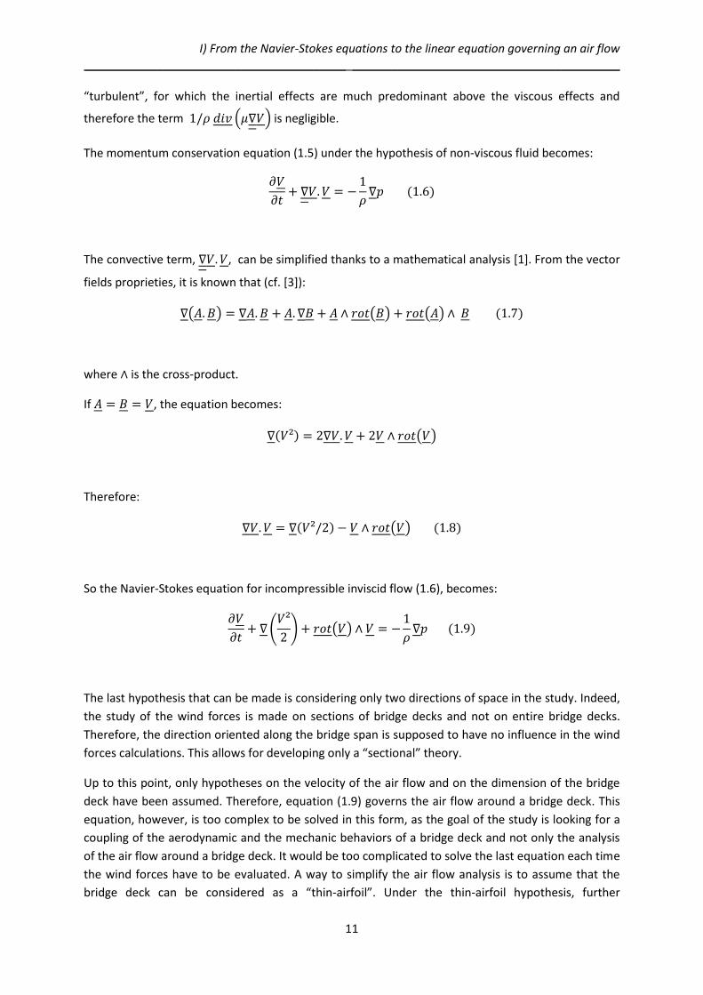
“turbulent”, for which the inertial effects are much predominant above the viscous effects and
therefore the term is negligible.
The momentum conservation equation (1.5) under the hypothesis of non-viscous fluid becomes:
The convective term, , can be simplified thanks to a mathematical analysis [1]. From the vector
fields proprieties, it is known that (cf. [3]):
where is the cross-product.
If , the equation becomes:
Therefore:
So the Navier-Stokes equation for incompressible inviscid flow (1.6), becomes:
The last hypothesis that can be made is considering only two directions of space in the study. Indeed,
the study of the wind forces is made on sections of bridge decks and not on entire bridge decks.
Therefore, the direction oriented along the bridge span is supposed to have no influence in the wind
forces calculations. This allows for developing only a “sectional” theory.
Up to this point, only hypotheses on the velocity of the air flow and on the dimension of the bridge
deck have been assumed. Therefore, equation (1.9) governs the air flow around a bridge deck. This
equation, however, is too complex to be solved in this form, as the goal of the study is looking for a
coupling of the aerodynamic and the mechanic behaviors of a bridge deck and not only the analysis
of the air flow around a bridge deck. It would be too complicated to solve the last equation each time
the wind forces have to be evaluated. A way to simplify the air flow analysis is to assume that the
bridge deck can be considered as a “thin-airfoil”. Under the thin-airfoil hypothesis, further

I) From the Navier-Stokes equations to the linear equation governing an air flow ________________________________________ _________________________________________
12
simplifications on the Navier-Stokes equations can be made. In the next paragraph, the implications
connected to considering an airfoil as thin and whether it can be correct to consider a bridge deck as
thin-airfoil will be explained.
c) The thin-airfoil theory
The major hypothesis made when considering an airfoil as thin is the irrotationality of the air flow
around the airfoil. The flow far ahead of the airfoil is parallel: the wind velocity is always oriented
along one single direction, even if this direction may vary in time. When the wind comes across an
obstacle, it is deviated and it is observed that the flow develops components perpendicular to the
wind orientation in order to pass the obstacle (cf. Figure 2 and the streamlines around an obstacle). If
the flow after the obstacle is parallel again, the flow is said to be “irrotational” and it may be
considered that the vortex part is worth zero [1]. So and equation (1.7) becomes:
The “irrotational” behavior of the air flow means that the vortexes created by the profile (as a
vertical speed component always appears around the profile) vanish without the need of viscosity.
This means that there is no separation of the flow from the profile and therefore, that vortexes are
not created in the wake of the profile. The irrotationality of an air flow around an obstacle depends
only on the obstacle itself (geometry, aspect ratio, surface material).
The analysis of the different components of the wind velocity allows making some additional
simplifications. The air flow around the bridge deck due to the wind is composed of four elements,
cf. [4]:
- the average horizontal wind velocity U ex
- the variations due to the turbulence of the wind far away ahead of the bridge deck (u ex , w ez)
- the speed variations of the air flow due to the bridge deck geometry (w1’ ex , w3’ ez)
- the speed variations of the bridge deck position due to its motion ( , )
The referential (ex , eZ) in which all these speeds have been written is fixed and horizontally/vertically
oriented.

I) From the Navier-Stokes equations to the linear equation governing an air flow ________________________________________ _________________________________________
13
Figure 1: Scheme of the cross-section of a bridge deck and definition of the motion variables
In order to be able to make the additional simplifications, the wind has to be considered in a special
way, as in [5] and [6]: the wind is horizontal and constant with respect to the bridge deck. The wind
turbulence and the motion of the bridge deck are included in the angle of attack of the bridge deck,
by the formula, as in [4]:
The term is added to the “regular” angle of attack of the bridge deck, .
Therefore, all the calculations will be done in the absolute referential (ex , ey), which corresponds to
the bridge deck referential at rest and not in the referential of the bridge deck when oscillating.
Under the new formulation of the air flow speeds, the velocity of the air around the bridge deck is
equal to V=(U+w1’) ex + w3’ eZ . In order to linearize the equation, the following inequalities are
assumed: and . This is the hypothesis of small perturbation.
As the flow is irrotational, the velocity of air can be derived from a potential, . The introduction of
the potential is made possible because if , then it comes that (the
rotational of a gradient is worth zero, cf. [3] for the demonstration).
The flow is incompressible ( , as seen in I.a) ) and so, .

I) From the Navier-Stokes equations to the linear equation governing an air flow ________________________________________ _________________________________________
14
The equation in two-dimension under the previous hypotheses can be written:
And the equation can be expressed as:
Rewriting the equation of mass quantity conservation (1.8) with the potential , it comes:
From the Schwarz theorem, the temporal and spatial derivates can be exchanged:
So the term inside the gradient is a space constant called F(t).
The space constant F(t) is evaluated considering being far away from the bridge deck. With the
hypotheses made before, it is known that far away from the bridge deck, the pressure is constant
and worth zero, because the pressure, , is the difference between absolute pressure (far away from
the bridge deck it is the pressure at rest) and pressure at rest. The velocity is a time and space
constant, U, so is a space constant too.
The unique term which is a non-zero far away from the bridge deck is:

I) From the Navier-Stokes equations to the linear equation governing an air flow ________________________________________ _________________________________________
15
So, F(t) can be expressed as:
Therefore, equation (1.13) becomes:
Under the hypothesis of small perturbation, the term becomes:
Changing the expression of the speed potential into by:
it comes:
Therefore equation (1.15) becomes:
A linear equation (1.17) has been obtained, as the pressure (which is the force by unit of surface
applied by the wind on the profile) is linear with respect to the speed potential. This equation is the
basis for the linear aeroelastic theory developed by [5] and [6] about oscillations of thin-airfoils in an
incompressible flow.
The final linear equation is true under the following hypothesis:
- subsonic flow (M<0.4)
- perfect fluid: its Lame’s constants are zero so it is non-viscous and incompressible
- irrotational flow (known as the Kutta condition)

I) From the Navier-Stokes equations to the linear equation governing an air flow ________________________________________ _________________________________________
16
- some wind speed approximations
- small perturbation of the flow around the bridge deck
Without studying all the mathematical steps required to pass from this equation of the pressure as a
function of the air velocity potential to the integrated forces due to an air flow on an airfoil, the
theoretical results obtained from the last equation will be developed and explained in chapter III).
In the case of a bridge deck, the two biggest approximations are the small perturbation and the
irrotationality of the flow. These hypotheses depend both largely on the shape of the airfoil (here the
bridge deck) and so and on the fact that the airfoil can be considered as a thin-airfoil or not. A thin-
airfoil is an airfoil with the following geometric properties:
- a little aspect ratio that ensures little perturbations of the flow around the airfoil. The aspect ratio is
defined by the height divided by the length.
- no singularities (such as angles) that may create a separation of the flow from the airfoil and violate
the Kutta condition
Figure 2: Air flow respecting the Kutta condition, without separation. Figure from [7]
Figure 3: Air flow not respecting the Kutta conditions. A separation of the boundary layer from the profile can be noticed. Figure from [7]
boundary layer
boundary layer
Position of the separation of
the flow often unstable
Position of the separation of
the flow located at the edge

I) From the Navier-Stokes equations to the linear equation governing an air flow ________________________________________ _________________________________________
17
Clearly, a “classic” bridge deck (cf. the Akashi Kaikyō Bridge cross-section, Figure 4) does not verify
the geometrical conditions required to be considered as a thin-airfoil because it always has
singularities and an aspect ratio too high. Some modern suspension bridges have decks that are so
thin that they become close to the thin-airfoil conditions. The thinner a bridge deck cross-section is,
the more it can be considered that the air flow is governed by a linear equation such as (1.17). For
example, the Normandy Bridge (Figure 5) has a very aerodynamic shape. In some cases, having a
bridge deck that can nearly be considered a thin-airfoil is done by purpose, in order to better control
the effect of the wind on the structure, by evaluating it thanks to the thin-airfoil theory. In other
cases, the philosophy may be, on the opposite, to create as many singularities as possible, in order to
avoid being to close to the Kutta conditions and so avoid any phenomenon of excessive wind forces.
But a bridge deck never perfectly respects the Kutta conditions, as it always needs road equipments
for the safety of the people crossing the bridge that create a separation of the flow from the bridge
deck on its extrados.
Figure 4: The Akashi Kaikyō Bridge cross-section: a clearly non-aerodynamic profile. Figure from [8]
Figure 5: The Normandy Bridge cross-section: an aerodynamic profile. Figure from [7]
The only forces that are considered in the study are the pressure forces applied by the air on the
profile. These elementary forces are oriented perpendicularly to the surface of the profile. The
shearing forces (also called skin friction) which are the tangential forces are neglected as the viscosity
of the fluid has been neglected previously

I) From the Navier-Stokes equations to the linear equation governing an air flow ________________________________________ _________________________________________
18
d) Dimensional analysis of the Navier-Stokes equation for an incompressible flow
Another way to simplify the Navier-Stokes equations is to transform it into a dimensionless equation.
This means dividing every physical variable by a typical constant, i.e., a constant that best
approximate the variable.
The Navier-Stokes equation for an incompressible flow
can be transformed into a dimensionless one, using the following changes of variable, where the
highlighted variable, , are the dimensionless ones.
Where L is a typical length. It could be the bridge deck width, B. is a typical velocity. It could be U,
the mean wind velocity. is a typical volumetric force, in this case, it is worth 0. And is the
density of air.
By replacing the variable by the dimensionless ones, it comes the following equation:
Where is the Reynolds number and is the Froude number.
In the studied cases, bridge decks, the Reynolds number is much bigger than one and so it can be
considered infinite. The volumetric forces are worth zero and so the Froude number is infinite.
Therefore it comes the same equation than the one found in I.b), under a dimensionless form:

I) From the Navier-Stokes equations to the linear equation governing an air flow ________________________________________ _________________________________________
19
Conclusion:
In this chapter, the hypotheses under which one can pass from the fundamental equations of fluid
mechanics, the Navier-Stokes equations, to the equation governing an air flow around a bridge deck
have been highlighted. In paragraph c), a linear equation has been obtained in the thin-airfoil theory.
This equation is the basis of the aeroelastic theory that will be developed further, in chapter III). It
has also been exposed that a bridge deck cross-section can never be considered as thin. Therefore,
the fundamental idea of aeroelasticity applied to bridges is that even if the decks are not thin, the
linearity of the wind forces with respect to the motion of the bridge can still be assumed.
20
II) An introduction to aerodynamics
After having considered only the mechanics of air in chapter I), in this chapter, the aerodynamic
theories will be introduced. Aerodynamics is the branch of physics that studies the interaction arising
from relative motion between air and a moving structure. This interaction can be considered as a
weak coupling which means that only the influence of the air on the structure (or the opposite) is
considered or as a strong coupling in which we have to consider the mechanics of both phases
(gaseous and solid, i.e. air and structure) at the same time because they interact. Aerodynamics
theories have been developed especially for studying the flight of airplanes but can also be applied to
civil structures to study the influence of the wind on deformable structures such as a slender bridge
deck or a cable (power line or bridge cable or stay).
a) Steady-state aerodynamics
In the steady-state aerodynamics, the interaction of an air flow horizontal and constant on a profile is
studied, assuming that the profile moves slowly enough to consider it fixed and to assume that the
flow is steady. The profile moves so slowly that the profile can be considered as fixed at any time
from the point of view of the fluid. This means that when the profile motion parameters change, the
flow reaches instantaneously the time-domain equilibrium. This is a weak coupling: the forces on the
profile depend only on the air parameters and on the profile present configuration. It is not
considered that the wind forces may induce a change of the profile parameters and is it not
considered that the time-history of the profile motion may have an influence on the wind forces at
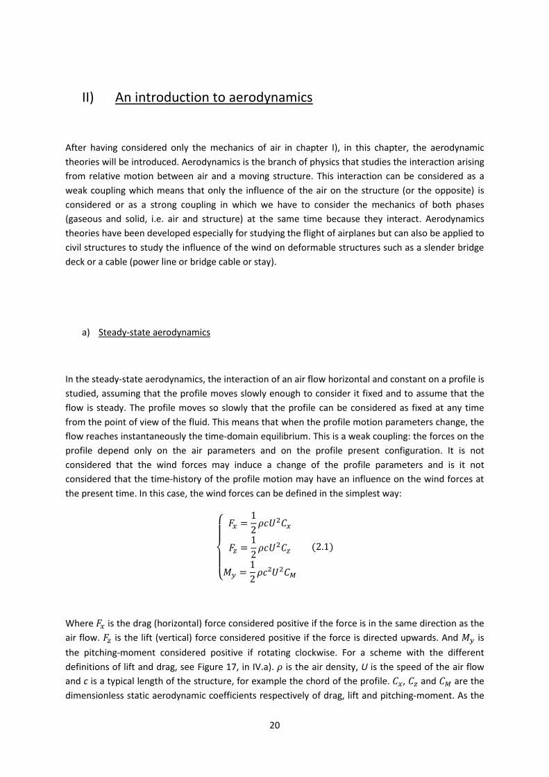
the present time. In this case, the wind forces can be defined in the simplest way:
Where is the drag (horizontal) force considered positive if the force is in the same direction as the
air flow. is the lift (vertical) force considered positive if the force is directed upwards. And is
the pitching-moment considered positive if rotating clockwise. For a scheme with the different
definitions of lift and drag, see Figure 17, in IV.a). is the air density, U is the speed of the air flow
and c is a typical length of the structure, for example the chord of the profile. , and are the
dimensionless static aerodynamic coefficients respectively of drag, lift and pitching-moment. As the

II) An introduction to aerodynamics ________________________________________ _________________________________________
21
static aerodynamic coefficients are dimensionless, the wind forces are expressed in N/m and the
pitching-moment is in Nm/m. These are forces on a section of bridge deck and so, forces per unit of
length. The forces of lift and drag and the pitching-moment are applied on the elastic center of the
profile, G. In the studied case, a bridge deck, the profile is symmetrical, so the elastic center is in the
middle of the profile.
From [1], one knows that the static aerodynamic coefficients are functions of the Reynolds number,
e=Uc/, the Strouhal number, k=ωc/U, also called reduced frequency, the Mach number, M=U/c,
the shape of the profile and the angle of attack. We have made the hypothesis that the flow is
perfect, so the influence of e is negligible. The Strouhal number is equal to zero as the profile is
considered fixed. As noticed experimentally, the dependency on the speed of the flow is neglected.
So in steady-state aerodynamics, the static aerodynamic coefficients are functions only of the angle
of attack and of the shape of the profile. So, for a given profile, the pitching-moment and the two
forces acting on the profile can be evaluated with the three static aerodynamic coefficients which are
functions only of the angle of attack.
Figure 6: Static aerodynamic coefficients for the “Viaduc de Millau” deck as a function of the angle of attack in degrees. The circles represent the value during the construction, the squares, once finished.
Figure from [7]

II) An introduction to aerodynamics ________________________________________ _________________________________________
22
Figure 7: a thin-airfoil scheme with classic nomenclature. G is the elastic center. O is the point of application of the wind forces. F is the aerodynamic center.
By defining some specific points of the profile, such as the pressure center and the aerodynamic
center and evaluating their position on the horizontal axis of the profile (cf. Figure 7), one may better
understand how are acting the forces on the profile.
The center of pressure, 0, is defined as the point of application of the aerodynamic forces,
considering only the lift forces. Therefore, the pitching-moment evaluated with respect to P is worth
zero. Respecting the conventions of sign, the distance from the leading edge to the pressure center,
is equal to:
The aerodynamic center, F, is the point on the chord about which the aerodynamic moment is
independent of the angle of attack. With the distance from the leading edge to the aerodynamic
center, the pitching-moment with respect to F is:
Introducing the aerodynamic coefficients, it comes the following expression:
Using the expression of :

II) An introduction to aerodynamics ________________________________________ _________________________________________
23
Deriving this expression and using the fact that the moment MF does not depend on the angle of
attack, in F:
As verified experimentally (cf. [7]) for little values of the angle of attack (not more than 5° of
amplitude), it can be assumed that the derivates of the static aerodynamic coefficients in =0 is a
constant. Therefore, the position of the aerodynamic center does not vary with the angle of attack.
And so:
If the thin-airfoil conditions are respected, it is known from theory, cf. [9], that:
and that
Therefore, the following relation between the aerodynamic coefficients of lift and pitching moment
is obtained:
Where a is the dimensionless distance between the middle of the profile and the elastic center of the
profile. In the case of a symmetrical profile, as in the case of a bridge deck, a=0.
b) Notion of reduced frequency
If now one considers that the profile is moving, in order to estimate if the coupling between the air
flow and the profile is weak or strong, a dimensionless quantity is introduced: the reduced frequency
which depends on the frequency of oscillation, the dimension of the studied profile and on the air
speed.

II) An introduction to aerodynamics ________________________________________ _________________________________________
24
Where is the reduced frequency, c is a typical length in the problem (like the chord of the profile),
U is the speed of the flow and TS is the frequency of oscillation of the profile.
A high reduced frequency, , means that the structure configuration changes faster than the
wind one: if a perturbation in the air flow is created at the leading edge of the profile, the profile
motion will have substantially changed when the perturbation will arrive at the end of the profile.
This kind of interaction may happen only for high frequencies of oscillation of the solid body. This
field of study is called vibro-acoustics.
A reduced frequency close to one means a high coupling between air flow and structure motion. One
may observe high motion amplitudes in air and in the structure. The behavior of both may become
non-linear.
A low reduced frequency means that the structure configuration changes more slowly than
the wind one. The behavior of the air influences the structure motion. The air flow can be considered
as steady, and the quasi-steady theory of aerodynamics may be used, with the static aerodynamic
coefficients as introduced in the previous paragraph.
In the case of a bridge deck, a typical length is between 10 and 30 m, a typical velocity, U between 10
and 70 m/s and a frequency of oscillation around 1s. This corresponds to a reduced frequency in the
range 0.14-3, which means that a strong coupling of the air and of the structure motion has to be
considered.
Different kind of interactions between air and structure may happen in the case of a bridge deck
subjected to wind:
- The Turbulence Induced Vibrations, also called TIV. The air turbulences (vertical or horizontal
gusts) create the phenomenon of buffeting that may induce vibrations of the bridge deck.
- The Movement Induced Vibrations, also called MIV. When moving, the structure modifies
the air flow around itself. By its motion, the bridge deck may create wind forces even
superior and induce a phenomenon of resonance, with high amplitudes of oscillation of the
bridge deck.
- The Vortex Induced Vibrations, also called VIV. In this case, the forces are due only to the air
flow and not the bridge deck motion. A vortex trail appears behind the structure, at a given
frequency, like in Figure 8. This vortex trail is not too dangerous if the frequency of the vortex
trail does not correspond to a natural frequency of oscillation of the bridge deck. If it is so,
the structure and the vortex trail may create a phenomenon of resonance, with high
amplitudes of oscillation of the structure.

II) An introduction to aerodynamics ________________________________________ _________________________________________
25
Figure 8: Vortex trail in water tunnel behind a circular cylinder. Figure from [10]
Figure 9: Different kind of behaviors for the law amplitude of oscillation as a function of the wind speed, for different profiles. Figure from [7]

II) An introduction to aerodynamics ________________________________________ _________________________________________
26
In Figure 9, a reassuming of the different behaviors of the bridge decks that may be observed is
exposed. All of the three kinds of interactions will not exist for all the bridges. For the wind speeds
they are subjected to, some bridge decks, will never encounter the VIV, for example.
In practice, bridge decks are designed in order to try to stay in the case represented by the first graph
in Figure 9. To do so, it must be verified that the MIV would appear only for wind speeds that are not
reached on the site and that the mechanical frequencies and the vortex frequencies do not
correspond, to avoid the VIV.

27
III) Wind forces in the frequency-domain: flutter derivatives
In the previous chapter, the steady-state aerodynamic theory has been introduced and the limits of
the steady-state approximation for an air flow on a moving structure have been detailed thanks to
the reduced frequency. For a bridge deck, such a hypothesis is not valid; the coupling of air and
structure has to be studied by taking into account the motion of the structure and not only its
present angle of attack. The flutter derivatives are functions that link the motion of the structure
with the induced wind forces, assuming that the forces are linear with respect to the structure
motion parameters.
Two approaches are possible at this point. The first one is the quasi-steady theory under which the
flutter derivatives are constants. In the quasi-steady theory, the flutter derivatives are calculated
using the static aerodynamic coefficients, considering only the present motion parameters (position
and velocity) of the bridge deck. In the second one, the coupling that is considered is more complex,
so, the wind forces at the present time depend on the present motion of the bridge deck but also on
its time-history motion. In this case, a way to link the complete motion of the bridge deck with the
induced forces is to evaluate the forces due to forced harmonic oscillations of the bridge deck. In the
second case, the flutter derivatives are functions of the frequency of the structure oscillation. If the
flow respects the Kutta condition, the expression of the flutter derivatives can be found analytically
with the Fung theory. If it does not, the expression has to be found experimentally as done by
Scanlan.
a) Steady forces and forced linearization of the equation
In a steady flow, as seen in II.a), the wind forces and moment applied on a profile by a constant and
horizontal air flow are:
Where is the density of air, U is the speed of the steady flow, c is a typical length of the structure (A
special care has to be taken in order to always consider the same length, like, for example, the width
of the bridge deck) and , and are the dimensionless static aerodynamic
coefficients of drag, lift and pitching-moment respectively.

III) Wind forces in the frequency-domain: flutter derivatives ________________________________________ _________________________________________
28
The wind forces are assumed to be functions of only two parameters of the bridge deck: the vertical
motion, z, and the rotation, α, also called angle of attack. The horizontal motion of the bridge deck, x,
is neglected as it has a much smaller influence than the vertical motion and the angle of attack.
Having a horizontal motion of the bridge deck is like increasing or reducing the incident horizontal
wind velocity on the bridge deck:
Where is the incident wind velocity as felt by the bridge deck, U is the absolute incident wind
velocity and is the horizontal bridge velocity. In practice, as , the influence of is neglected
and it is considered that . Moreover, the stiffness of a bridge deck is much bigger in the
horizontal direction and so its displacements are smaller than in the vertical direction.
The drag is often not considered either in the flutter derivatives theories applied to bridges. It is
evaluated with the static aerodynamic coefficients. This difference of treatment is due to the fact
that the drag does not create phenomenon of resonance whereas the lift or the pitching moment
may resonate with the torsional and heaving modes of the bridge deck. So, one does not look for the
same sensitivity for the interaction between drag and mechanical behavior of the bridge. As no
resonance phenomenon is encountered for the drag, a static evaluation of the wind forces is enough
to size the bridge deck for horizontal wind forces.
In the flutter derivatives theory, the wind forces linearity with respect to the structure motion is
assumed, so one may write that:
Where and are the flutter derivatives. They link the lift, and the pitching-moment, , with
the motion parameters of the bridge deck, , the angle of attack, , the velocity of the angle of
attack, , the vertical displacement of the bridge deck and , its vertical velocity. With is indicated
a time derivation.
One may see this approximation as a Taylor series approximation, as the functions are linearized
around the equilibrium position. The equilibrium position corresponds to the position at rest. So, the
linearization is made with respect to the four motions parameters at , , and
(cf. [7]):
III) Wind forces in the frequency-domain: flutter derivatives ________________________________________ _________________________________________
29
Therefore, there is a correspondence between the flutter derivatives in equation (3.3) and the
derivates of the wind forces with respect to the motion parameters in equation (3.4). For example,
considering the lift:
b) An example of the quasi-steady theory: forces on a galloping cylinder with flutter derivatives
for a low reduced frequency
In order to illustrate the quasi-steady theory, a practical case will be analyzed: the wind forces on a
cable of diameter D. The quasi-steady theory is much more appropriate for a cable than for a bridge
deck, as for the same frequency of oscillation of the cable and the same mean velocity of the wind,
the reduced frequency is lower, because the typical dimension is smaller. For a bridge deck, the
typical dimension is in the range 10-30m, for a cable, it is around 20 cm. So, the reduced frequency,
, is 100 times smaller and can be considered as much smaller than 1.
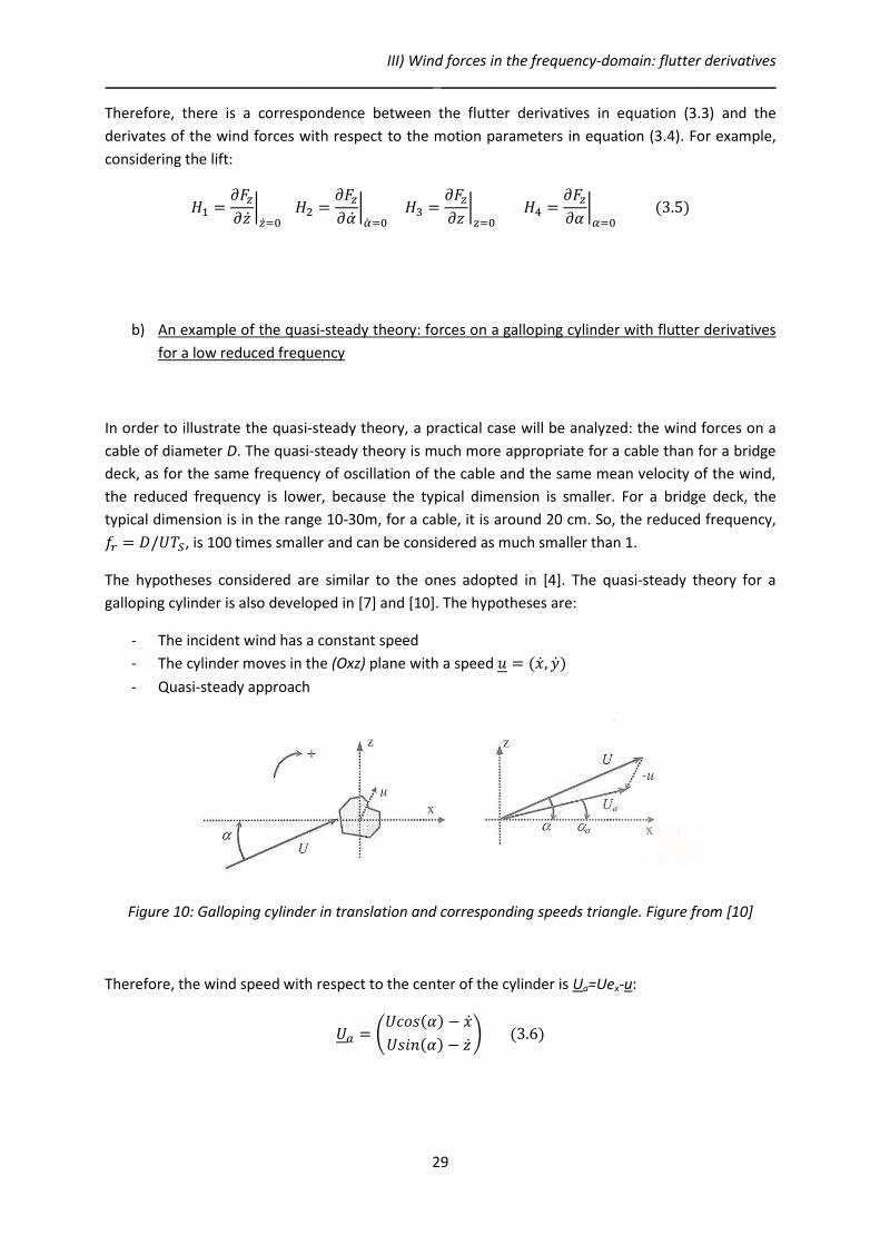
The hypotheses considered are similar to the ones adopted in [4]. The quasi-steady theory for a
galloping cylinder is also developed in [7] and [10]. The hypotheses are:
- The incident wind has a constant speed
- The cylinder moves in the (Oxz) plane with a speed
- Quasi-steady approach
Figure 10: Galloping cylinder in translation and corresponding speeds triangle. Figure from [10]
Therefore, the wind speed with respect to the center of the cylinder is Ua=Uex-u:
III) Wind forces in the frequency-domain: flutter derivatives ________________________________________ _________________________________________
30
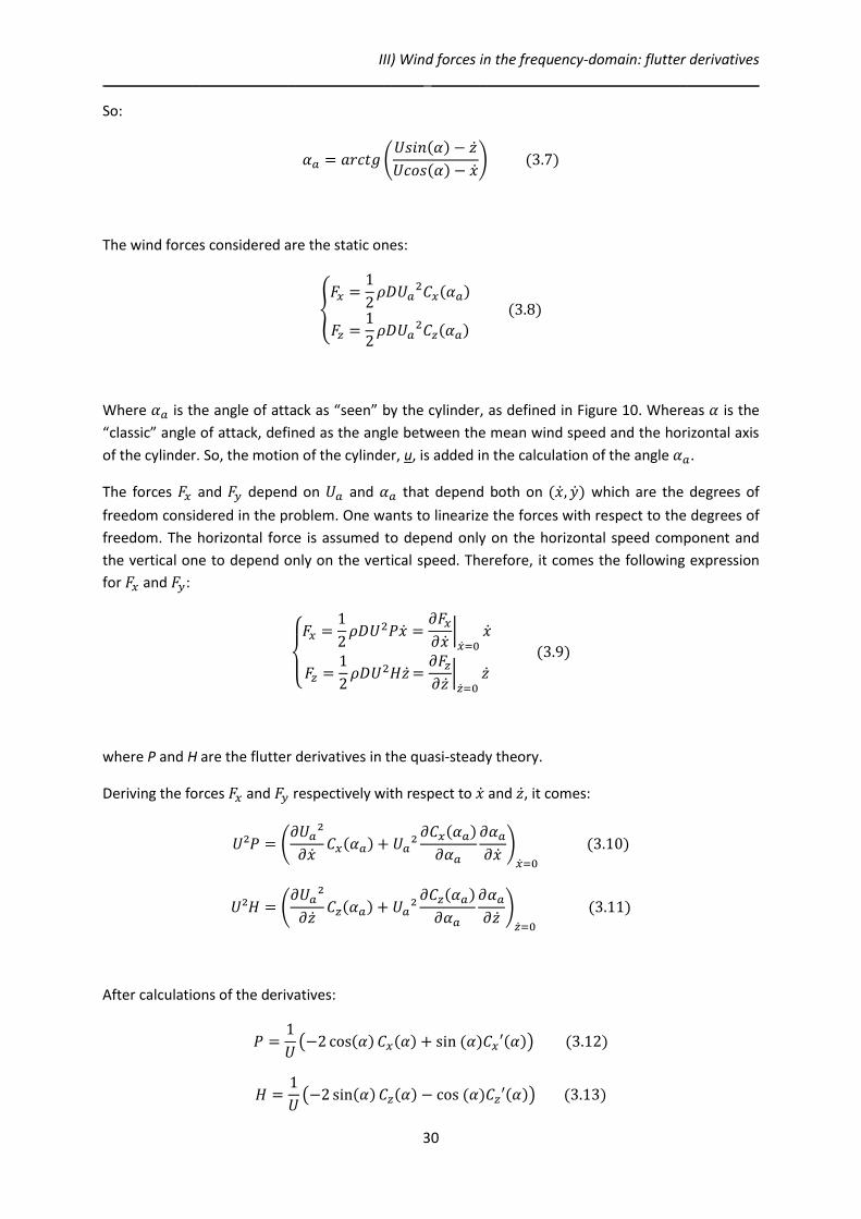
So:
The wind forces considered are the static ones:
Where is the angle of attack as “seen” by the cylinder, as defined in Figure 10. Whereas is the
“classic” angle of attack, defined as the angle between the mean wind speed and the horizontal axis
of the cylinder. So, the motion of the cylinder, u, is added in the calculation of the angle .
The forces and depend on and that depend both on which are the degrees of
freedom considered in the problem. One wants to linearize the forces with respect to the degrees of
freedom. The horizontal force is assumed to depend only on the horizontal speed component and
the vertical one to depend only on the vertical speed. Therefore, it comes the following expression
for and :
where P and H are the flutter derivatives in the quasi-steady theory.
Deriving the forces and respectively with respect to and , it comes:
After calculations of the derivatives:

III) Wind forces in the frequency-domain: flutter derivatives ________________________________________ _________________________________________
31
An expression of the flutter derivatives depending only on the static aerodynamic coefficients of the
profile and on the instantaneous value of the angle of attack has been obtained.
This procedure is similar to the one used in [4]. Indeed, one could also derive the forces with respect
to the turbulences of the wind (u, w), considering them in the evaluation of and , by defining
the wind speed as:
Where U is the mean wind velocity and u and w are the horizontal and vertical air gusts.
Doing so, one would have found an expression of and under the following form:
still considering separately the horizontal and vertical forces and motion parameters.
The crossed components which express the dependency of the forces in a direction with respect to
the motion in the other direction may also be added to this expression, like the dependency of
with respect to and w, for example.
c) Coupling of aerodynamic and mechanical behavior for a reduced frequency close to 1
As seen in II.b), for a reduced frequency around 1, like for a bridge deck, the coupling between
aerodynamic and mechanical behaviors requires a more complex formulation than the quasi-steady
one to be modeled. Therefore, the aerodynamic forces have to be considered as depending on the
time-history motion of the airfoil. A way to understand this dependency is to consider the wind
forces as a function of the frequency of the bridge deck oscillation.
The expression of the linearized forces remains the same for forced harmonic oscillations if the
problem respects the Kutta conditions, as demonstrated by Theodorsen in 1935 and detailed by Fung
in [6]:

III) Wind forces in the frequency-domain: flutter derivatives ________________________________________ _________________________________________
32
This expression is valid only for harmonic oscillations of the bridge deck parameters, , the angle of
attack and z, the vertical displacement of the bridge deck. Now, the flutter derivatives which are
named with an #, depend on the dimensionless pulsation of oscillation, , where b is the
half-chord of the profile and ω is the pulsation of oscillation of the profile. The half-chord of a profile
is half the distance between the leading edge and the trailing edge.
The flutter derivatives ,
and ,
are the “in phase” components. The flutter derivatives ,
and
, are the “quadrature” components. This means that the response to a bridge deck
motion has a part which oscillates proportionally to the motion of the bridge deck and a part that
oscillates with a difference of phase of /2. If the motion is a cosine, the in phase component will be
proportional to a cosine too and the quadrature component will be proportional to a sine. Therefore,
the response (the wind forces) to an oscillation of the motion parameters of the bridge deck for a
given frequency can also be defined by an amplitude and a phase differences. Cf. VII.a) for the steps
required to pass from the flutter derivatives to the expression of the amplitude and the phase
difference.
The exact expression of these flutter derivatives can be found with complicated calculations, under
the hypothesis of small perturbation of the flow and irrotationality of the flow (Kutta condition). This
hypotheses allow to do a potential approach for solving the aerodynamic equation (1.17) that has
been found in I.c). These calculations are done in [6] by Fung assuming harmonic oscillations of the
airfoil and using the Theodorsen function :
Figure 11: Real part F(k) and imaginary part G(k) of the Theodorsen function. Figure from [7]
III) Wind forces in the frequency-domain: flutter derivatives ________________________________________ _________________________________________
33
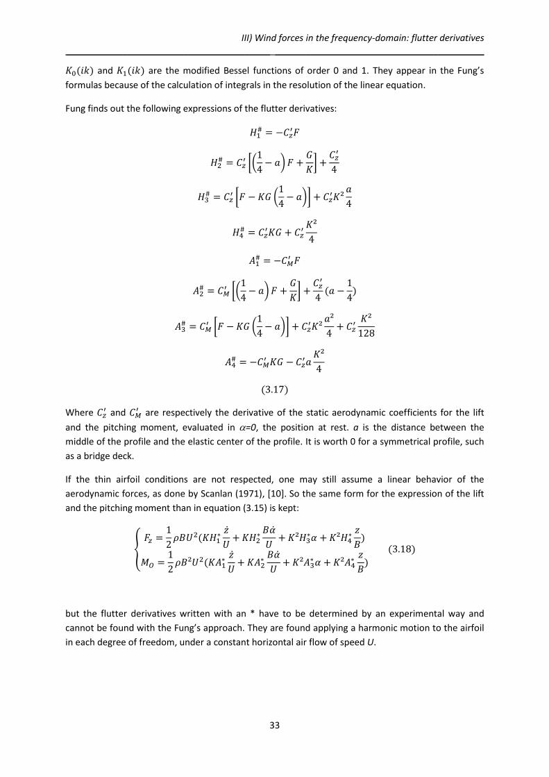
and are the modified Bessel functions of order 0 and 1. They appear in the Fung’s
formulas because of the calculation of integrals in the resolution of the linear equation.
Fung finds out the following expressions of the flutter derivatives:
Where and
are respectively the derivative of the static aerodynamic coefficients for the lift
and the pitching moment, evaluated in =0, the position at rest. a is the distance between the
middle of the profile and the elastic center of the profile. It is worth 0 for a symmetrical profile, such
as a bridge deck.
If the thin airfoil conditions are not respected, one may still assume a linear behavior of the
aerodynamic forces, as done by Scanlan (1971), [10]. So the same form for the expression of the lift
and the pitching moment than in equation (3.15) is kept:
but the flutter derivatives written with an * have to be determined by an experimental way and
cannot be found with the Fung’s approach. They are found applying a harmonic motion to the airfoil
in each degree of freedom, under a constant horizontal air flow of speed U.

III) Wind forces in the frequency-domain: flutter derivatives ________________________________________ _________________________________________
34
d) Determination of bridge deck aerodynamic coefficients
The determination of bridge deck aerodynamics coefficients can be done in two ways: an
experimental way, using a wind tunnel or a computational way, using a CFD (Computational Fluid
Dynamic) software. The accuracy of the evaluation of the flutter derivatives and of the static
aerodynamic coefficients is determinant for the quality of the analysis of the wind effects on
structures.
1) Wind tunnels experiments
The most common way for the determination of the aerodynamic coefficients is the wind tunnel
analysis. This analysis requires the construction of a reduced geometric scale model which is
subjected to an air flow in a wind tunnel. In order to find the true wind forces on the bridge deck
even if one works on a model, some characteristics of the air flow and bridge deck should be kept
similar to reality. The physical similitude needed for a proper correspondence between the reality
and the experimentation results is called the “similarity” criteria. These criteria are based on a
dimensional analysis of the wind forces.
The principle of the dimensional analysis for the similarity criteria applied to wind tunnel
experiments is more detailed in [1] and [10].
From the Navier-Stokes equations, it is known that the wind forces depend on 6 parameters, , the
air density, D, a typical dimension of the bridge deck, U, the flow velocity, n, some frequency, , the
fluid viscosity and g, the gravitational acceleration. F, the wind force is assumed to be dimensionally
related to all of the 6 parameters through the following dimensional relation:
Where the symbol means “dimensionally consistent”. , , , , , are exponents to be
determined. All these 6 parameters are dimensionally functions of only 3 basic quantities: mass, M,
length, L and time, T. So the equation (3.19) becomes:
From this dimensional relation, by equating corresponding exponents for mass, length and time:
III) Wind forces in the frequency-domain: flutter derivatives ________________________________________ _________________________________________
35
Considering some coefficients as functions of others
The force F can be dimensionally expressed as:
or
From this analysis, it follows that the dimensionless force is a function of the following
dimensionless numbers:
- , also known as the Strouhal number if n corresponds to the frequency of vortex
shedding from a bluff objective. If n corresponds to nm, a mechanical frequency, is
called the reduced frequency. - is the reciprocal of the Reynolds number. - is the Froude number
This analysis helps understand which coefficients are important to be considered when passing from
a reduced geometry scale model to a full-scale model.
If one wants the aerodynamic behavior of the reduced scale geometry to correspond exactly to the
reality of the bridge deck, the three dimensionless numbers should have the same value in both
cases. Passing from the model to the real bridge deck, three scale factors appear: a length scale
(geometric scale of the model), a velocity scale (ratio real wind speed over speed of the air flow in
the tunnel) and a density scale (ratio air over the liquid or gas used in the tunnel). For example, if one
uses a wind tunnel working with air in atmospheric conditions, the density scale will be worth one
and, necessarily, one of the three dimensionless numbers will not be equal in both cases. Therefore,
it is often not possible to have the three dimensionless numbers equal in both cases (reality and wind
tunnel) as only one or two scale factors can be adjusted. Anyway, the experience of the laboratory
engineers is fundamental to control the suitability of the experiment.

III) Wind forces in the frequency-domain: flutter derivatives ________________________________________ _________________________________________
36
2) Computational fluid dynamic
This paragraph is inspired by a document from the INRIA [11] and an interview with Mr. Frédéric
Bourquin [12].
Another way to determine the aerodynamic characteristics of a profile is to develop a model of the
air flow around the profile with a CFD (Computational fluid dynamic) software. Once known the air
flow around the model, the pressure around the profile can be integrated and the air forces on the
profile evaluated. One can do static or dynamic model, by moving or not the profile.
The CFD softwares solve numerically the Navier-stokes equations in two dimensions, as the studied
profiles are assumed to be infinitely extended. Even if solving numerically the Navier-Stokes
equations is quite heavy in term of calculation and time requested, some interesting results can be
obtained with this tool. The INRIA (Institut National de Recherche en Informatique et en
Automatique) has tried to develop it with simple profile such as cylinders (Figure 12) or rectangular
prisms (Figure 13).
Figure 12: Periodic vortex shedding created by a cylinder in an incompressible air flow after a transient phase.

III) Wind forces in the frequency-domain: flutter derivatives ________________________________________ _________________________________________
37
Figure 13: Drag and lift of a rectangular profile oscillating harmonically in an incompressible air flow. After a transient time, it can be noticed that the drag and lift oscillate harmonically, with the same
period as the rectangular profile.
Conclusion :
In this chapter, two different approaches to the flutter derivatives have been exposed: the quasi-
steady one, in which the flutter derivatives depend on the static aerodynamic coefficients and the
frequency-dependency one, in which the flutter derivatives depend on the frequency of oscillation of
the bridge deck. The quasi-steady theory has been applied to a cable to understand how the wind
forces could be linearized to define the flutter derivatives. The equations for the flutter derivatives as
a function of the frequency of oscillation have been found by Thedorsen in the 30’s; in the thin-airfoil
conditions, for a harmonic oscillation of the airfoil, the flutter derivatives link the wind forces and the
airfoil motion linearly, by creating amplitude and phase differences between the forced oscillation
and the wind forces. These are the flutter derivatives named with an # which can be found
theoretically. For a bridge deck which cannot be considered as thin, Scanlan has made the hypothesis
that the wind forces are still linked to the bridge deck motion by the same analytical expression as
the Theodorsen’s one. But the flutter derivatives are named with an * and should be found
experimentally. Finally, in paragraph III.d), experimental and numerical ways to evaluate the
aerodynamic coefficients have been outlined.

38
IV) Wind forces in the time-domain: indicial functions
In the previous chapter, an approach to the wind forces in the frequency-domain with the flutter
derivatives has been studied. Since purpose of the work is to make a time-domain modelling of the
wind force, in the following chapter, the notion of indicial functions will be introduced. These
functions link the wind forces with the time-history motion of profiles, like the flutter derivatives link
the wind forces with the frequency of oscillation of profiles.
In paragraph a), an infinitesimal approach to the indicial functions will be done. It helps understand
and define what an indicial function is. In paragraphs b), c) and d), the lift as a function of the vertical
motion of a bridge deck will be approached with indicial functions by three different ways. The first
approach in paragraph b) is inspired by the article of Scanlan [13]; the definition of indicial functions
on the basis of the flutter derivatives will be given. After having defined the Fourier transform (cf. 1st
Appendix), in paragraph c), the wind forces will be defined as a convolution product between the
indicial functions and the time-history motion of the bridge deck. In paragraph d), a final approach to
the indicial functions will be made with the Duhamel’s integral. In this approach, it will be clarified
under which hypotheses the theory of the indicial functions can be considered true. In paragraph e),
a reassuming of the three ways used to define the indicial functions and a comparison of the
approaches are made. Finally, in paragraph f), the complete wind forces will be expressed with the
Fourier transform: the lift and the pitching-moment as a function of both the angle of attack and the
vertical motion of the bridge deck.
a) Infinitesimal approach
With the flutter derivatives, the fact that wind forces do not depend only on the instantaneous
parameters of the airfoil motion anymore has already been considered. In the case of a single degree
of freedom (the angle of attack of the airfoil, for example), the lift acting on the airfoil is the sum of
contributes given by the previous angles. In the frequency-dependent flutter derivatives theory, the
forces at a time t can be obtained only if the angle of attack is oscillating harmonically. In this
chapter, the angle of attack time-history is considered random.
Going backwards to the steady approach, the lift is equal to:
This corresponds with an airfoil motion where , which means that the airfoil is moving slowly.
This allows making a quasi-steady development. It is also assumed that the variations of the angle of
attack of the bridge deck are in the range ±5° and so that the derivate of the static aerodynamic
coefficients in =0 are constant, as made in II.a). Therefore, a Maclaurin expansion of the static

IV) Wind forces in the time-domain: indicial functions __________________________________________________________________________________
39
aerodynamic coefficient can be made for the lift that allows transforming the lift as a function of the
angle of attack into a Taylor series limited to the first term:
Where is a constant:
Doing this Maclaurin expansion is like assuming that the lift as a function of the angle of attack is a
linear function.
Now, the airfoil is considered moving too fast and so, the quasi-steady theory is not valid anymore.
For example, if one applies an abrupt step-function change from a zero lift condition to an
incremental angle of attack worth 0 at the airfoil at the time t=0, the lift will undergo a transient
change (cf. Figure 14 for the pitching-moment) because the flow needs a certain time before it can
be considered as steady again. The vortexes created at the edges because of the abrupt change of
angle of attack need to flow along the profile before reaching stabilization of the flow again (cf.
Figure 15). In this non-steady case, a certain linearity of the lift with respect to the angle of attack
may still be considered, by modelling the transient phase by the following equation:
Where s=2Ut/B is the dimensionless time as defined by Theodorsen and is an indicial lift-growth
function. Now, the linearity is between the amplitude of the angle of attack, , and the transient
response to it. In the thin-airfoil hypotheses, in 1925, Wagner has proved that equation (4.a.3) is
valid and has also found the theoretical expression of the indicial function (cf. Figure 16 for the
shape of the indicial function). The indicial function as defined by Wagner is consistent with the
quasi-steady approach, as for s tending to , tends to 1. So, for an infinite time value which
corresponds to a stabilization of the flow, the lift is worth:
as in equation (4.a.2).
IV) Wind forces in the time-domain: indicial functions __________________________________________________________________________________
40
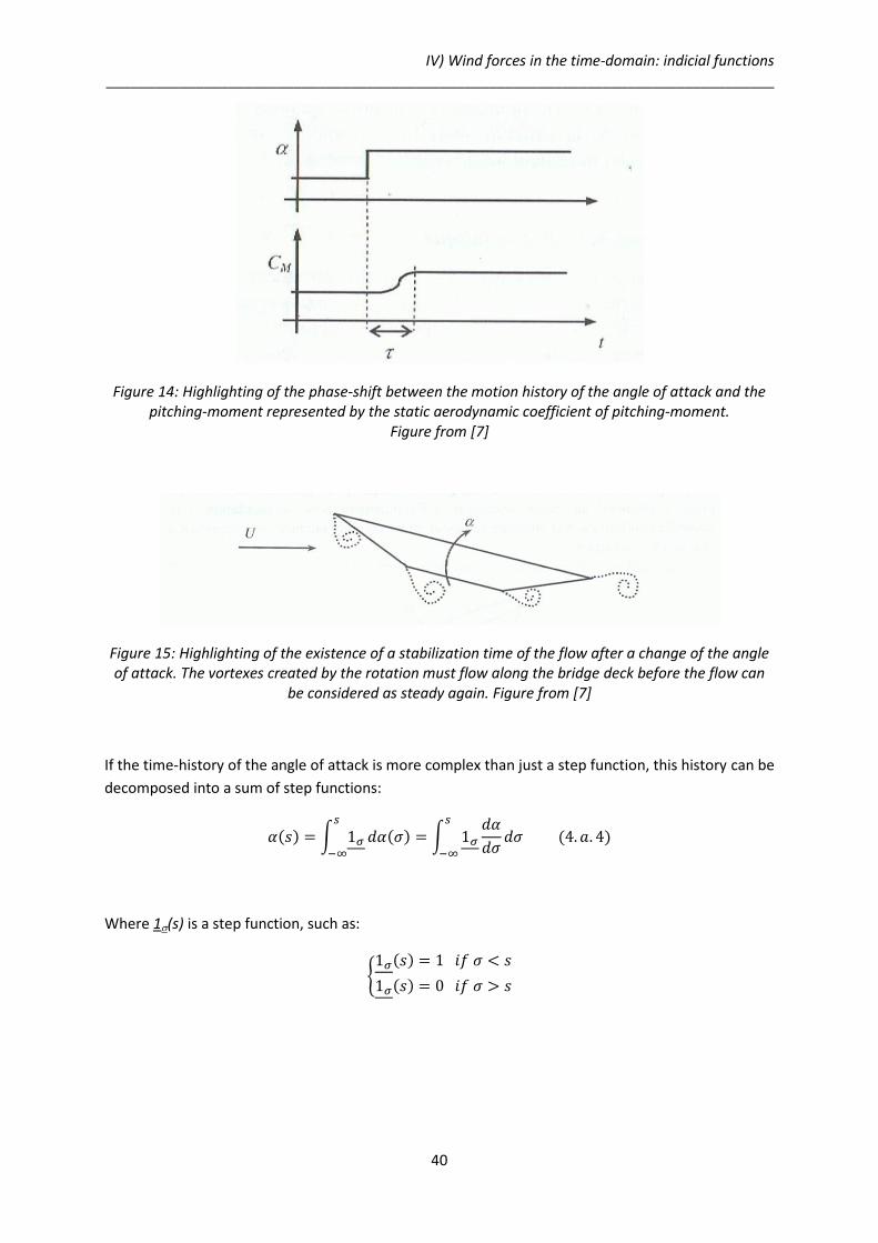
Figure 14: Highlighting of the phase-shift between the motion history of the angle of attack and the pitching-moment represented by the static aerodynamic coefficient of pitching-moment.
Figure from [7]
Figure 15: Highlighting of the existence of a stabilization time of the flow after a change of the angle of attack. The vortexes created by the rotation must flow along the bridge deck before the flow can
be considered as steady again. Figure from [7]
If the time-history of the angle of attack is more complex than just a step function, this history can be
decomposed into a sum of step functions:
Where 1(s) is a step function, such as:

IV) Wind forces in the time-domain: indicial functions __________________________________________________________________________________
41
If the system respects the linear superposition principle, the lift at the present time can be expressed
as a function of the time-history of the angle of attack, using equation (4.a.3) and the decomposition
of the time-history of the angle of attack (4.a.4):
Cf. pargraph IV.d), about the Duhamel integral applied to the indicial functions, for more
explanations about the decomposition of the time-history of the angle of attack, the superposition
principle and the underlying hypotheses.
Through integration by part, it comes:
And, with a change of variable, :
This expression written only for the lift forces in function of the angle of attack may be also assumed
for the moment, under a similar form.
Assuming that the forces are linear with respect to the vertical velocity of the airfoil, as well as they
are linear with respect to the angle of attack, both lift and pitching moment can be expressed as
function of the angle of attack and the vertical velocity in the same way.
In doing this reasoning, it is assumed that the system respects the superposition principle which is
the condition for integrating the infinitesimal forces and assuming that the indicial functions are
constants in time. These hypotheses have been proved to be true by Wagner in 1925, for the thin-
airfoil condition. Even if the thin-airfoil condition is not respected, it is assumed that the expression
of the lift can be written in the same way, with indicial functions. But new expressions of the indicial
functions should be found, as the ones found by Wagner theoretically are no longer exact in the
studied case:

IV) Wind forces in the time-domain: indicial functions __________________________________________________________________________________
42
Where are the indicial response functions in the case of a bridge deck section which is not a thin-
airfoil. They should be found experimentally. q=1/2.U² is the dynamic pressure. Equation (4.a.8) is
also assumed by Costa and Borri in [14].
Figure 16: Indicial response functions: Wagner ( ) and real function in the case of a bridge deck ( ). Figure from 13
In the next paragraph, it will be proved that the analytical expressions of the indicial functions can be
obtained from the flutter derivatives. But these analytical expressions are not easy to use in practice
as they contain integrals that should be calculated each time it is required to evaluate the value of
the functions for a given time. According to [14] and [5], in order to fasten the use of an indicial
function, an empiric expression that approximates the indicial function can be used. This empiric
function, as given by Scanlan, is a sum of exponential groups depending on five parameters:

IV) Wind forces in the time-domain: indicial functions __________________________________________________________________________________
43
If the derivative of the indicial functions is need, one simply derives expression (4.a.9) and obtains:
The Wagner’s indicial function, (s), that gives the lift for an abrupt change of the value of the angle
of attack has been approximated by R.T. Jones in 1940 under the form (4.a.10) with the following
values for the 4 coefficients used in the derivative formula: , ,
and , cf. [13].
Depending on the complexity of the shape of the indicial function, one exponential group or, on the
contrary, three or four groups, may be required to approximate an indicial function under the form
of a sum of exponential groups in a proper way.
Going backwards to equation (4.a.8), it may be surprising that the wind forces need to be defined as
an integral from - to the present time s. This would mean that the present forces are linked to the
motion of the bridge deck even a long time before the present time. This may create a problem of
convergence of the result, because an infinite time-history is needed to evaluate the true forces
acting on the bridge deck at the present time. In fact, the shape of the indicial forces allows making a
simplification on the integral. Considering the lift as a function of the angle of attack, one can notice
from Figure 16 that the indicial function, , tends to 1 for s tending to and so, that the derivative
of the indicial function, ’, tends to 0 for s tending to . Therefore, one may assume that after a
certain time that will be called sL, the integration time, the indicial function may be approximated by
the constant 1 and its derivative by the constant 0. Therefore, equation (4.a.8) may be re-written as:
If the integrated form of the lift is considered, as in equation (4.a.5),
the same simplification on the integral may be made:
as for an infinite time, the airfoil is assumed at rest.
IV) Wind forces in the time-domain: indicial functions __________________________________________________________________________________
44
According to [15], a correct integration time is . For such an integration time, the convolution
integral is always convergent. The fading memory effect allows forgetting what happened in the
time-history motion of the bridge deck before this integration time.
b) Finding the expression of indicial functions – Scanlan’s approach
In this paragraph, an expression of the Fourier transform of indicial functions as a function of the
flutter derivatives will be determined.
In the case of the study of the wind force as a function of the angle of attack and of the vertical
motion of the airfoil, for harmonic oscillations, the following relation (from the Scanlan’s flutter
derivatives formula) can be used, as seen in paragraph III.c):
Where K=Bω/U is the reduced velocity and ω is the pulsation of oscillation.
As the motion of the airfoil is harmonic, the expression may be re-formulated by noticing that:
Therefore, the lift can be expressed as a function only of the vertical motion of the bridge deck and
the angle of attack:
As ω=UK/B, the expression of the lift may be rearranged:

IV) Wind forces in the time-domain: indicial functions __________________________________________________________________________________
45
By analogy, the pitching moment becomes:
In paragraph IV.a), the expression of the lift and the moment as functions of the angle of attack and
the vertical motion of the airfoil has been assumed by analogy with the thin-airfoil theory. It gives the
wind forces for generic motions of the airfoil at the present dimensionless time, s:
With , one indicates the derivative with respect to the time, t. With ‘, one indicates the derivative
with respect to the dimensionless time, s.
At this point, two expressions of the wind forces have been obtained: one expression that is the
Scanlan equation, valid only for harmonic oscillations of the bridge deck, equation (4.b.4-5), and one
expression that has been assumed with the indicial functions, equation (4.b.6). If a harmonic motion
of the bridge motion parameters is also assumed in the second equation, one will be able to equal
between both expressions of the wind forces as functions of the motion parameters of the bridge
deck.
To simplify the understanding on how the expression of the indicial functions can be found thanks to
these two expressions of the wind forces, only the lift as the function of the vertical motion of the
airfoil will be considered. So equation (4.b.4) becomes:
Which can also be expressed as a function of :
Under a dimensionless form, and so, as a function of and with a change of variable as done for
equation (4.a.7), equation (4.b.6) becomes:

IV) Wind forces in the time-domain: indicial functions __________________________________________________________________________________
46
One can notice in Figure 16 that is not continuous in 0. It is worth 0 in and 0.5 in . So, as
is discontinuous in , one must decide whether means or .
If one decides that it means , the exact equation is, in fact:
The arbitrary choice made about the meaning of worth 0 will be discussed later in this paragraph.
As said previously, in order to compare these two expressions, a harmonic motion of the vertical
motion of the bridge deck is assumed, so:
Where ω is the pulsation of the harmonic motion, k=Bω/2U=K/2 is the reduced velocity, s=2Ut/B, the
dimensionless time and is the dimensionless amplitude of oscillation of the vertical speed motion
of the bridge deck:
Therefore, equation (4.b.8) becomes:
Calculating the lift with the harmonic motion for , as defined in equation (4.b.11), equation (4.b.10)
may be transformed:
Where is defined as:
. It is not the exact Fourier transform of the
derivative of the indicial function, , as the exact Fourier transform, , of would be:

IV) Wind forces in the time-domain: indicial functions __________________________________________________________________________________
47
Cf. 1st Appendix on the Fourier transform for the definition of the Fourier transform used in this
work. From - to 0-, is worth 0, so it s derivative is worth 0 too. The link between the exact
Fourier transform of and is just an additive constant:
So:
And, finally, the notation can be introduced in equation (4.b.13):
Previously, one had decided in the definition of the lift with the indicial functions, that if , the
integration variable was worth 0, it meant that it was worth 0+. If it had been decided that 0 meant 0-
, one would have obtained:
As , it comes that:
Assuming the same harmonic motion and defining as
which is the real Fourier transform of , it comes:
As it was predictable, the same equation as equation (4.b.16) for is obtained whether one
decides that means or .
For the rest of the study, the first definition of 0 will be kept, so 0 means 0+. So, as in equation
(4.b.13):
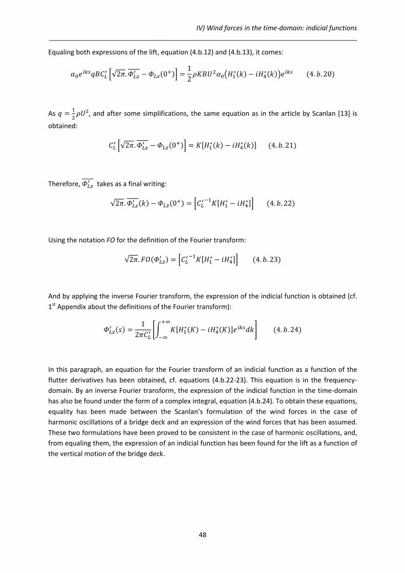
IV) Wind forces in the time-domain: indicial functions __________________________________________________________________________________
48
Equaling both expressions of the lift, equation (4.b.12) and (4.b.13), it comes:
As
, and after some simplifications, the same equation as in the article by Scanlan [13] is
obtained:
Therefore, takes as a final writing:
Using the notation FO for the definition of the Fourier transform:
And by applying the inverse Fourier transform, the expression of the indicial function is obtained (cf.
1st Appendix about the definitions of the Fourier transform):
In this paragraph, an equation for the Fourier transform of an indicial function as a function of the
flutter derivatives has been obtained, cf. equations (4.b.22-23). This equation is in the frequency-
domain. By an inverse Fourier transform, the expression of the indicial function in the time-domain
has also be found under the form of a complex integral, equation (4.b.24). To obtain these equations,
equality has been made between the Scanlan’s formulation of the wind forces in the case of
harmonic oscillations of a bridge deck and an expression of the wind forces that has been assumed.
These two formulations have been proved to be consistent in the case of harmonic oscillations, and,
from equaling them, the expression of an indicial function has been found for the lift as a function of
the vertical motion of the bridge deck.
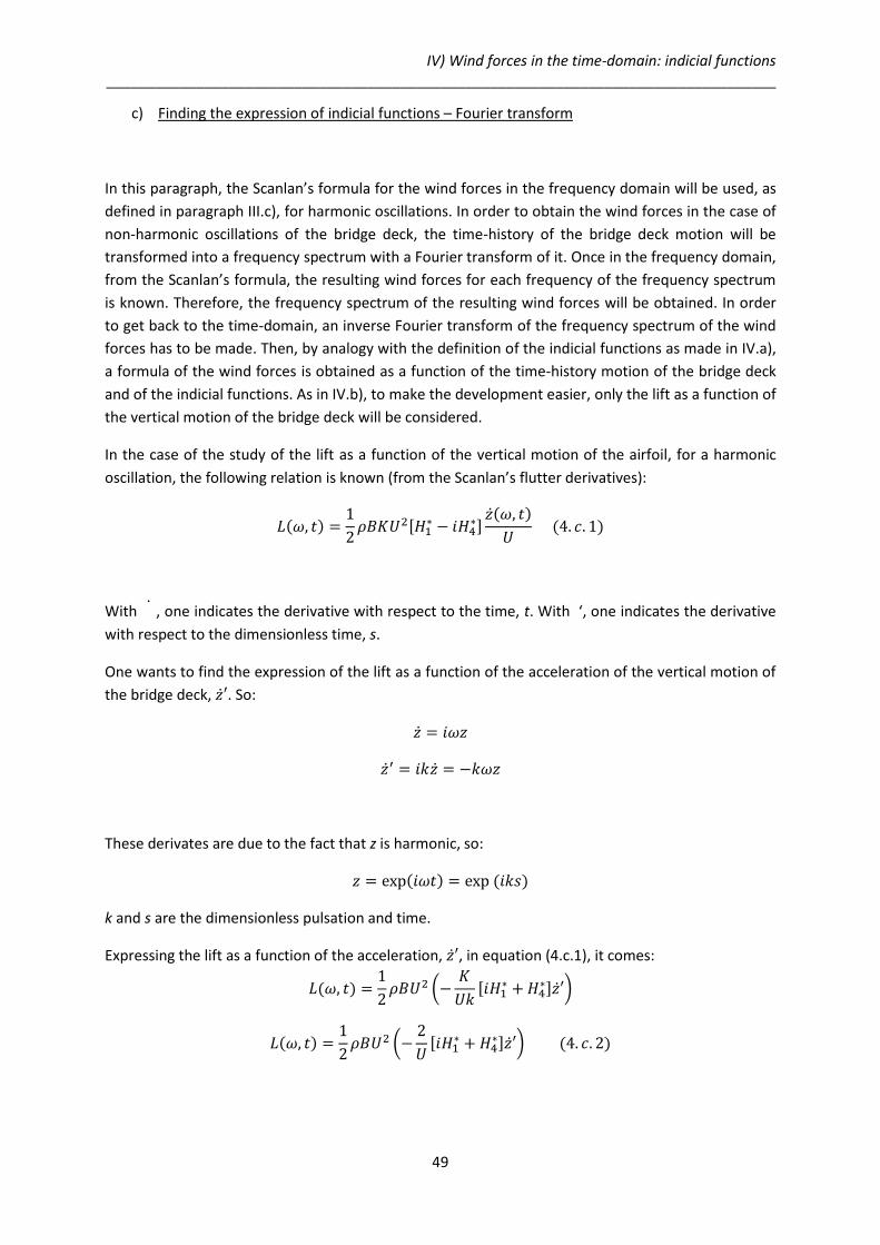
IV) Wind forces in the time-domain: indicial functions __________________________________________________________________________________
49
c) Finding the expression of indicial functions – Fourier transform
In this paragraph, the Scanlan’s formula for the wind forces in the frequency domain will be used, as
defined in paragraph III.c), for harmonic oscillations. In order to obtain the wind forces in the case of
non-harmonic oscillations of the bridge deck, the time-history of the bridge deck motion will be
transformed into a frequency spectrum with a Fourier transform of it. Once in the frequency domain,
from the Scanlan’s formula, the resulting wind forces for each frequency of the frequency spectrum
is known. Therefore, the frequency spectrum of the resulting wind forces will be obtained. In order
to get back to the time-domain, an inverse Fourier transform of the frequency spectrum of the wind
forces has to be made. Then, by analogy with the definition of the indicial functions as made in IV.a),
a formula of the wind forces is obtained as a function of the time-history motion of the bridge deck
and of the indicial functions. As in IV.b), to make the development easier, only the lift as a function of
the vertical motion of the bridge deck will be considered.
In the case of the study of the lift as a function of the vertical motion of the airfoil, for a harmonic
oscillation, the following relation is known (from the Scanlan’s flutter derivatives):
With , one indicates the derivative with respect to the time, t. With ‘, one indicates the derivative
with respect to the dimensionless time, s.
One wants to find the expression of the lift as a function of the acceleration of the vertical motion of
the bridge deck, . So:
These derivates are due to the fact that z is harmonic, so:
k and s are the dimensionless pulsation and time.
Expressing the lift as a function of the acceleration, , in equation (4.c.1), it comes:

IV) Wind forces in the time-domain: indicial functions __________________________________________________________________________________
50
The Fourier transform of , is worth:
is defined according to the 1st Appendix of this work. The time integration is done only till
the present time, s, because the time-history of the vertical motion is known only till s. is the
frequency spectrum of the vertical motion of the bridge deck. It represents the weight of each
frequency present in the time-history of the vertical motion.
Using the results found in the 1st Appendix and the equation in the frequency-domain (4.c.2), the
Fourier transform of the lift, FL, as a function of the frequency spectrum of the vertical motion is
equal to:
Equation (4.c.5) is similar to the theoretical results obtained in the article by Borri and Hoeffer in
2000, [16].
Now that the frequency spectrum of the lift, FL has been obtained to get back to the time-domain, an
inverse Fourier transform of FL should be made, as defined in the 1st Appendix. So, the lift force
equals to:
The studied functions and variables are smooth, as they are physical, so we can do some
modifications on the integral that has just been found,
Thanks to the modification on the integrals, now, the main integral is on the time-domain, instead of
an integral on the frequency-domain, as in (4.c.5). The integral on the frequency-domain still exists,

IV) Wind forces in the time-domain: indicial functions __________________________________________________________________________________
51
but should be evaluated first. The analytical form that has just been found in (4.c.6) for the lift, is a
convolution product between the inverse Fourier transform of
and the vertical
acceleration of the airfoil.
If one puts down that the integral on the frequency-domain is a function of time, it comes:
This formulation with such multiplicative constants has been chosen in order to be consistent with
the definition of the indicial functions as in IV.a). Therefore, is an indicial function.
With the introduction of the indicial function as defined in (4.c.7), equation (4.c.6) may be
transformed into:
With integration by part of equation (4.c.8):
, as at an infinite time, the airfoil is at rest. This result is similar to the formulation of
the lift as defined in IV.a).
In this paragraph, thanks to a Fourier transform of the vertical motion of the bridge deck, and using
the Scanlan’s formula in the frequency-domain, the Fourier transform of the lift has been obtained.
Then, with an inverse Fourier transform, the expression of the lift in the time-domain has been
found. Then, in order to find the same formulation for the lift as the one assumed in IV.a), the indicial
function, , has been identified. In this approach, it has not been assumed a particular
formulation for the lift. The final formulation is due to the Fourier transform and inverse transform
steps that can be written under the form of a convolution product.
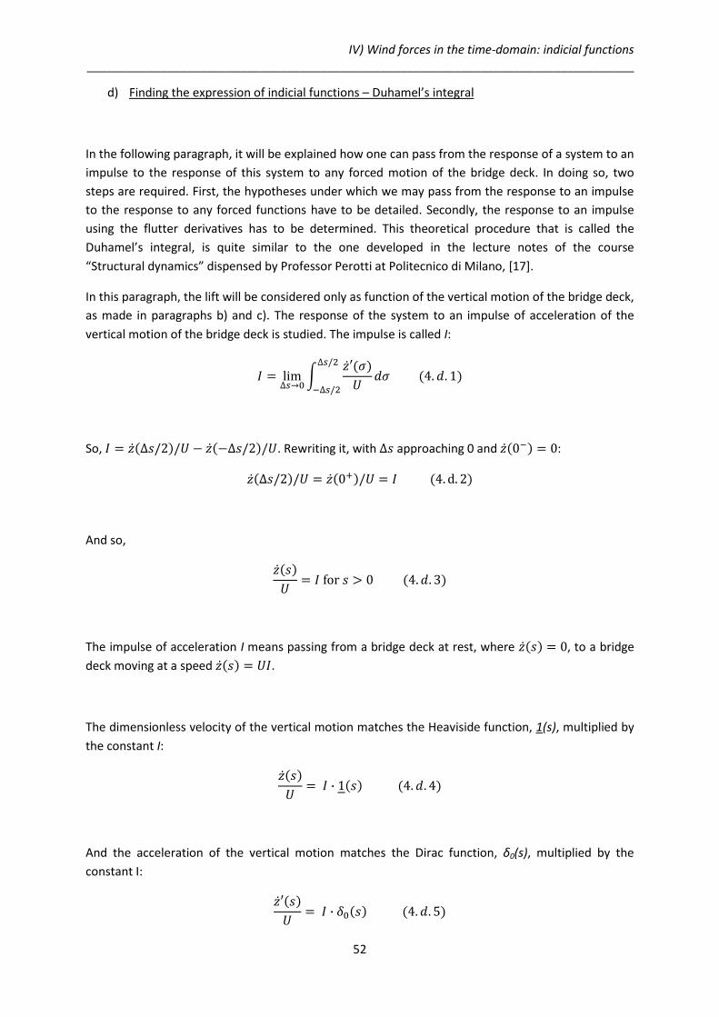
IV) Wind forces in the time-domain: indicial functions __________________________________________________________________________________
52
d) Finding the expression of indicial functions – Duhamel’s integral
In the following paragraph, it will be explained how one can pass from the response of a system to an
impulse to the response of this system to any forced motion of the bridge deck. In doing so, two
steps are required. First, the hypotheses under which we may pass from the response to an impulse
to the response to any forced functions have to be detailed. Secondly, the response to an impulse
using the flutter derivatives has to be determined. This theoretical procedure that is called the
Duhamel’s integral, is quite similar to the one developed in the lecture notes of the course
“Structural dynamics” dispensed by Professor Perotti at Politecnico di Milano, [17].
In this paragraph, the lift will be considered only as function of the vertical motion of the bridge deck,
as made in paragraphs b) and c). The response of the system to an impulse of acceleration of the
vertical motion of the bridge deck is studied. The impulse is called I:
So, . Rewriting it, with approaching 0 and :
And so,
The impulse of acceleration I means passing from a bridge deck at rest, where , to a bridge
deck moving at a speed .
The dimensionless velocity of the vertical motion matches the Heaviside function, 1(s), multiplied by
the constant I:
And the acceleration of the vertical motion matches the Dirac function, δ0(s), multiplied by the
constant I:

IV) Wind forces in the time-domain: indicial functions __________________________________________________________________________________
53
For the first part of the analysis, it is assumed that the response to an impulse of acceleration of the
vertical motion at a time 0 is known. This indicial response is called h(s). So:
The first major approximation that is made at this point is assuming that the response is proportional
to the amplitude of the impulse. This may be considered correct only for little oscillations of the
bridge deck. This is called the hypothesis of linearity.
If the impulse happens at a time , the response of the system will be the same as in equation
(4.d.4), with a translation of the time axis origin:
The second major hypothesis made by doing this translation in time is assuming that the system is
invariable in time. In practice, the wind forces on a bridge deck are studied on intervals of nearly 1
minute to 10 minutes maximum. So, one may assume that the bridge deck does not change in such
an interval of time.
The vertical velocity can always be approximated into an infinite sum of Heaviside functions changing
the continuous signal into a discrete one. To make this easier, we choose constant sampling time, .
The velocity of the vertical motion becomes:
The impulses I defined before now equal .
So, the acceleration is a sum of Dirac functions at the times :
It has been assumed that we know the response to an impulse. It has also been assumed that the
system is invariable in time and linear, so the response to the discrete vertical motion is equal to the
sum of the responses to each of the impulses at the times :

IV) Wind forces in the time-domain: indicial functions __________________________________________________________________________________
54
In doing this operation, the superposition principle is applied: the response to various stimuli is equal
to the sum of the responses which would have been caused by each stimulus individually. This
principle is linked to the linearity and to the invariance in time of the system.
The sum is limited to the time , as the response at a time depends only on the
previous configurations of the angle of attack (causality principle).
By transforming the sum into an integral and transforming the time intervals into infinitesimal
ones, , the Duhamel’s integral is obtained:
In equation (4.d.11), it has been found that the lift can be written in the form of a convolution
product between the time-history motion of the bridge deck and the response to an impulse, h(s).
With this approach, the indicial function corresponds with the response to a unitary impulse of the
velocity of the vertical motion, h(t).
Now, the response to an impulse has to be evaluated. To evaluate it, the results obtained in
paragraph b) of the 1st Appendix about the Fourier transform will be used. The impulse corresponds
to the Heaviside function, therefore, the response to an impulse is worth:
y(t) is the response to an impulse. In this case, it corresponds to h(t). The complex impedance,
is defined as:
Using, equation (4.c.2), it comes that:
Therefore, using dimensionless variables, equation (4.d.12) may be re-expressed for the studied case:

IV) Wind forces in the time-domain: indicial functions __________________________________________________________________________________
55
The function h(s) that has just been found is the response to an impulse. As equation (4.d.11) is
similar to the equation of the wind forces expressed with the indicial functions, in order to be
consistent with equation (4.a.8), is defined as:
and are proportional. The indicial function corresponds indeed to the response to an
impulse, as defined in paragraph IV.a).
Inserting the indicial function as defined in equation (4.d.16), the expression of the lift that has
just found can be re-written:
e) Comparison of the three ways used for the calculation of indicial functions
The lift as a function of the vertical motion of a bridge deck has been expressed in the time-domain
in three different ways: the Scanlan’s approach, the Fourier transform and the Duhamel’s integral. In
the three developments, the same expression for the lift has finally been obtained. The indicial
functions have always been defined in the same way,
for the indicial function and
for the derivate of the indicial function.
This definition of the indicial function that is consistent with the definition made in IV.a), allows
expressing the lift under the form of a convolution product:

IV) Wind forces in the time-domain: indicial functions __________________________________________________________________________________
56
These three different approaches are a way to ensure that the formulation of the problem is true:
first it has been verified that the wind forces could be expressed under the form as assumed in IV.a)
and secondly that the formulation of the indicial functions with the flutter derivatives and the
different multiplicative constants was true. But these different approaches reflect also different ways
to perceive the indicial functions.
In the Scanlan’s approach, the form of the wind forces has been assumed under the form of a
convolution product with indicial functions. Enforcing equality with the wind forces derived from the
flutter derivatives for an harmonic motion, the indicial function where identified as functions of the
flutter derivatives.
Since the wind forces were defined in the frequency-domain by the flutter derivatives in chapter III),
in the second approach, it has been decided to use the Fourier transform. Seeking the wind forces at
time t, the time-domain history-motion of the bridge deck has been transformed into the frequency
one. Then, the frequency spectrum thus obtained has been multiplied by the flutter derivatives for
each frequency of the spectrum. A back transformation in the time-domain with an inverse Fourier
transform provides the wind forces at time t. In this approach, it has been possible to identify the
indicial function and define it a posteriori, once the final expression of the lift forces is found in time
domain.
In the first part of the third approach, the Duhamel’s integral, it has been assumed that the response
of the system to an impulse was known, as done in paragraph IV.a). The different hypotheses that
allow passing from this indicial response valid for any time-history motions of the bridge deck to the
Duhamel’s convolution integral have been detailed. In the second part, the response to an impulse
with the Fourier transform has been evaluated. This third approach, through its hypotheses, allowed
perceiving the limits of the indicial functions theory which are the linearity and the time invariance of
the studied system.
f) Complete expression of lift and pitching moment with indicial functions
In this part, the lift and pitching moment will be expressed with indicial functions thanks to the
second approach studied, the Fourier transform. As done in the second approach, a Fourier
transform of the time-history motion of the bridge deck will be done. Then, the frequency spectrum
will be multiplied by the flutter derivatives. The Fourier transformation of the wind forces is
transformed back in the time-domain by an inverse Fourier transform.
Using the well-known Scanlan’s formula of the flutter derivatives for harmonic oscillation of the
airfoil:

IV) Wind forces in the time-domain: indicial functions __________________________________________________________________________________
57
The motion of the bridge deck is harmonic, therefore, the different motion parameters of the bridge
deck can be expressed only with the angle of attack and vertical velocity of the bridge deck:
With , one indicates the derivative with respect to the time, t.
As ω=UK/B, the lift becomes:
Expressing and as functions of the reduced velocity k=Bω/2U and s=2Ut/B:
With ‘, one indicates the derivative with respect to the dimensionless time, s.
Expressing the lift as a function of and , with 2k=K, it comes:
By analogy, for the pitching moment:
Therefore, the Fourier transform of the lift, FL, and of the moment, FM, can be expressed with the
Fourier transform of , FZ2, and of ’, FA1. These expressions correspond with the article by Borri
and Hoeffer, [16]:

IV) Wind forces in the time-domain: indicial functions __________________________________________________________________________________
58
Considering the lift:
where,
Because of the causality principle, the bridge deck motion is known only till the present time, s. So
the time integration of the Fourier transform of the time-history motion of the bridge deck is limited
from to s.
Applying the inverse Fourier transform:
After calculation, the time-domain lift can be expressed as a function of the motion of the bridge
deck and the flutter derivatives:
As the studied functions are smooth, some modifications can be done on the integral that has just
been found.

IV) Wind forces in the time-domain: indicial functions __________________________________________________________________________________
59
As lift and pitching moment almost have the same expression, by analogy, the expression of the
pitching moment can also be obtained:
In order to simplify the calculation, the following expressions are put down:
With these functions that have been introduced, the lift and the pitching moment can be written in a
more simple way:
With integration by part:

IV) Wind forces in the time-domain: indicial functions __________________________________________________________________________________
60
In , the system is at rest, the bridge deck is steady, so:
By analogy, for the pitching moment, it comes:
This final expression of the wind forces corresponds to the definition of the wind forces made in IV.a)
with the indicial functions. The function i that have been identified are the indicial functions.
Conclusion:
In this chapter, it has been shown how the wind forces can be expressed in the time-domain thanks
to the indicial functions. All through the chapter, different ways to approach the indicial functions
and different properties of these functions have been discovered. The link between the indicial
functions and the flutter derivatives has been made, in the frequency-domain and in the time-
domain, in three different ways. The limits of this linear formulation that has been assumed being
true by analogy with the thin-airfoil theory, have been tackled. Finally, in the last paragraph, the
complete wind forces have been expressed by defining the four different indicial functions.

61
V) Practical expression of the wind forces acting on a bridge
deck
In the last chapter, we have expressed the wind forces due to the motion of the bridge deck. These
forces have to be integrated in the complete system of the wind forces acting on the bridge deck.
Some approximations have to be made to define the wind and the wind forces in order to make the
analysis easier and faster. The choices we have made are similar to the choices made in [14]. They
offer a good approximation for a first approach to the indicial functions. The main hypotheses made
are to consider the horizontal part of the wind field constant, to neglect the horizontal movement of
the bridge deck and to consider the drag as a steady-state load.
a) Wind model
We assume that the bridge deck is immersed in a turbulent, incompressible and non-viscous wind
field. In the wind velocity, , we distinguish the mean wind velocity which depends only of the
position of the measurement of the wind field and the turbulent wind velocity which depends on the
position and the time of the measurement and whose mean is equal to zero.
Where is the mean of the wind velocity. is the mean wind speed and is the
turbulent perturbation. M is a general point of coordinates (x,y,z).
So,
The mean velocity is oriented along the x-axis which corresponds to the horizontal direction:

V) Practical expression of the wind forces acting on a bridge deck __________________________________________________________________________________
62
The turbulent velocity has components on the three direction of space. So,
where u, v and w are the turbulent components oriented respectively along the x-axis, the y-axis and
the z-axis.
Figure 17: Section scheme. With drag, FD, and lift, FL, defined in the referential of the profile
The y-axis is defined as the axis along the bridge span. The z-axis is defined as the vertical axis,
perpendicular to the bridge deck at rest. The x-axis is the horizontal axis along the bridge deck at
rest. G, the origin, is the elastic center of the bridge deck.
For the evaluation of the wind forces on the bridge deck, we consider the bridge deck as a profile
which means that we consider only two dimensions of space. We study a cross-section which is
assumed infinitely extended. Therefore, the y-axis direction is not taken into account. The forces that
we have to evaluate are three: the horizontal force on the profile along the x-axis, also called drag,
the vertical force along the z-axis, also called the lift force and a moment around the y-axis, also
called pitching moment.
b) Wind forces
The wind load acting on the bridge deck cross-section is expressed as a sum of three components:
- the quasi-static part
- the self-excited part which depends on the motion of the bridge deck
- the buffeting part which depends on the turbulence of the incoming wind velocity
V) Practical expression of the wind forces acting on a bridge deck __________________________________________________________________________________
63
Where is the vertical wind force, along the z-axis, is the horizontal wind force, along the
x-axis and is the aerodynamic moment. The subscripts (0), (se) and (b) indicate respectively
the quasi-static, self-excited and buffeting components.
Depending on the definition of and , and may not correspond respectively to
the lift, L and the drag, D. What is called lift may whether be the force “vertical” with respect to the
moving bridge deck, so its orientation is rotated of the angle of attack α with respect to the z-axis (as
defined on Figure 17), or whether be the absolute vertical force, along the z-axis. For the drag, we
can find both definitions too, whether it is the “horizontal” force with respect to the bridge deck,
rotated of an angle α, or whether it is the absolute horizontal force, along the x-axis. In order to
know what the definitions of the drag and lift are, we should consider carefully the definition of the
data of the aerodynamic coefficients (static aerodynamic coefficients and flutter derivatives).
Commonly, in the study of aerodynamics applied to bridges, the forces are defined in the absolute
referential, whereas in classical aerodynamics, the forces are defined in the airfoil referential, rotated
of an angle .
The aerodynamic moment, called , corresponds to the moment about the y-axis, . The
forces are defined with respect to the elastic center of the profile, G. Therefore, no additive moment
due to a possible change of the point of application of forces that may create a lever arm is to be
considered.
If drag and lift are orientated along with the bridge deck, we should rotate them in order to express
them in the absolute referential:
As the angle of attack remains small (some degrees), we consider that the cosine of is equal to 1
and that the sine of is equal to 0. So, no matter the definition of the drag and lift forces, we may
always consider that:
V) Practical expression of the wind forces acting on a bridge deck __________________________________________________________________________________
64
The quasi static part depends only on the angle of attack α and the mean horizontal velocity, U:
Where is the average wind speed, ρ is the air density and , and are the aerodynamic
coefficients.
The self-excited forces are linked to the motion of the bridge deck and can be expressed as seen in
IV) with indicial functions:
We use the same definition for the derivates than in IV): is the derivate of with respect to s, the
dimensionless time. The relation to pass from the real vertical velocity of the bridge deck to the
dimensionless one, , is:
Where and , so:
And:

V) Practical expression of the wind forces acting on a bridge deck __________________________________________________________________________________
65
The buffeting forces depend only on the turbulent part of the wind velocity. Considering that ,
we can neglect the horizontal component, u. As we do not consider the forces along the y-axis, the
only turbulence that we consider is w, the vertical one. The exact formulation of the buffeting load is
a Küssner-type formulation:
Where and are indicial functions similar to the indicial functions for the self-excited forces,
but for which, and .
Figure 18: comparison between the Küssner’s-type indicial function, , and the self-excited type
function, , as a function of dimensionless time, s. Figure from [13]
As done by Borri and Costa [14], we may approximate these Küssner-type indicial functions with the
Wagner-type ones: we consider that the turbulence is added to the vertical motion of the bridge
deck. So, to the vertical motion of the bridge, z’, we should add the vertical turbulence, as if the
bridge had a vertical motion equal to z’+w in a horizontal steady flow of velocity U. A particular
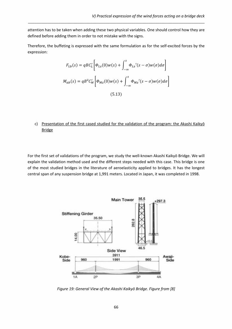
V) Practical expression of the wind forces acting on a bridge deck __________________________________________________________________________________
66
attention has to be taken when adding these two physical variables. One should control how they are
defined before adding them in order to not mistake with the signs.
Therefore, the buffeting is expressed with the same formulation as for the self-excited forces by the
expression:
c) Presentation of the first cased studied for the validation of the program: the Akashi Kaikyō
Bridge
For the first set of validations of the program, we study the well-known Akashi Kaikyō Bridge. We will
explain the validation method used and the different steps needed with this case. This bridge is one
of the most studied bridges in the literature of aeroelasticity applied to bridges. It has the longest
central span of any suspension bridge at 1,991 meters. Located in Japan, it was completed in 1998.
Figure 19: General View of the Akashi Kaikyō Bridge. Figure from [8]

V) Practical expression of the wind forces acting on a bridge deck __________________________________________________________________________________
67
1) Aerodynamic data
The data of the static aerodynamic coefficients have been taken from [18]: “Wind tunnel test of
Naboky-Bisan-Seto Bridges with stiffening truss” by Shin Narui. The static aerodynamic coefficients of
drag, lift and pitching moment are defined in the steady and absolute referential. So, in order to
obtain the forces in the mechanical referential, (Oxz), which is fixed, we do not need to rotate the
forces of an angle worth the angle of attack:
Figure 20: static aerodynamic coefficients of drag (CD), lift (CL) and pitching moment (CM) of the bridge
deck cross section of the Akashi Kaikyō Bridge central span as a function of the angle of attack

V) Practical expression of the wind forces acting on a bridge deck __________________________________________________________________________________
68
For the flutter derivatives, we have taken the data from the article [19], “Multi-mode flutter and
buffeting analysis of the Akashi-Kaikyō bridge”, by H. Katsuchi et al. In this case too, the wind forces
are defined in the absolute referential, (Oxz).
Figure 21: Flutter derivatives of lift (Hi) and pitching moment (Ai) of the bridge deck cross section of the Akashi Kaikyō Bridge central span.
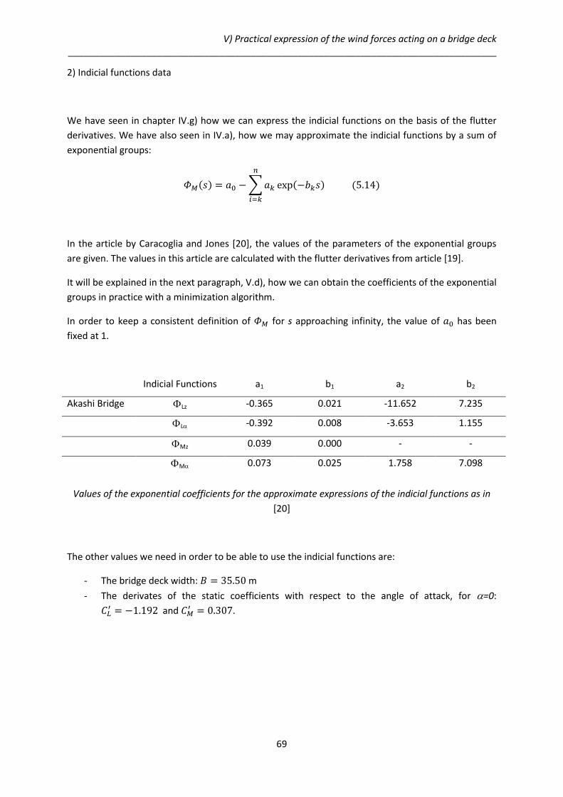
V) Practical expression of the wind forces acting on a bridge deck __________________________________________________________________________________
69
2) Indicial functions data
We have seen in chapter IV.g) how we can express the indicial functions on the basis of the flutter
derivatives. We have also seen in IV.a), how we may approximate the indicial functions by a sum of
exponential groups:
In the article by Caracoglia and Jones [20], the values of the parameters of the exponential groups
are given. The values in this article are calculated with the flutter derivatives from article [19].
It will be explained in the next paragraph, V.d), how we can obtain the coefficients of the exponential
groups in practice with a minimization algorithm.
In order to keep a consistent definition of for s approaching infinity, the value of has been
fixed at 1.
Indicial Functions a1 b1 a2 b2
Akashi Bridge Lz -0.365 0.021 -11.652 7.235
L -0.392 0.008 -3.653 1.155
Mz 0.039 0.000 - -
M 0.073 0.025 1.758 7.098
Values of the exponential coefficients for the approximate expressions of the indicial functions as in
[20]
The other values we need in order to be able to use the indicial functions are:
- The bridge deck width: m
- The derivates of the static coefficients with respect to the angle of attack, for =0:
and
.
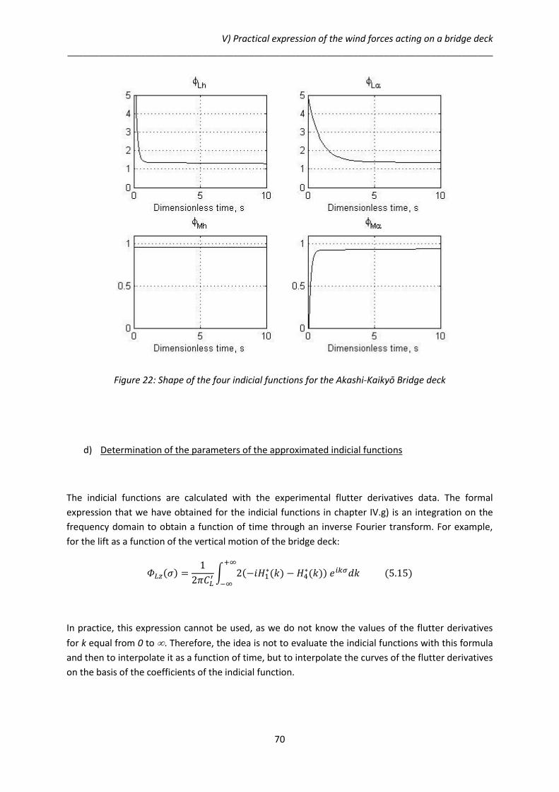
V) Practical expression of the wind forces acting on a bridge deck __________________________________________________________________________________
70
Figure 22: Shape of the four indicial functions for the Akashi-Kaikyō Bridge deck
d) Determination of the parameters of the approximated indicial functions
The indicial functions are calculated with the experimental flutter derivatives data. The formal
expression that we have obtained for the indicial functions in chapter IV.g) is an integration on the
frequency domain to obtain a function of time through an inverse Fourier transform. For example,
for the lift as a function of the vertical motion of the bridge deck:
In practice, this expression cannot be used, as we do not know the values of the flutter derivatives
for k equal from 0 to . Therefore, the idea is not to evaluate the indicial functions with this formula
and then to interpolate it as a function of time, but to interpolate the curves of the flutter derivatives
on the basis of the coefficients of the indicial function.

V) Practical expression of the wind forces acting on a bridge deck __________________________________________________________________________________
71
In IV.c), the Scanlan’s approach to indicial functions, we have obtained the following equation for the
lift as a function of the vertical motion of the bridge deck:
Where
.
If we use the approximate expression of the indicial function,
and apply the Fourier transform to this approximate expression:
The term is worth:
Separating the real part and the imaginary part:
With,

V) Practical expression of the wind forces acting on a bridge deck __________________________________________________________________________________
72
and using equation (5.16), we have two expressions of the same quantity, :
The flutter derivatives are determined experimentally for a given number of frequencies, kl. We have
to determine the coefficients of the indicial functions on the basis of these data. The identification of
the coefficients is performed in [20] through a non-linear least squares method, by minimizing the
squared-error function, also called residual. Still for the same case, the lift as a function of the
vertical motion, the residual is defined this way [21]:
With M, the number of frequencies for which the flutter derivatives have been measured
experimentally.
In the article [20], the number of exponential groups of the indicial function, n, may vary from 1 to 4.
It is determined by a statistical analysis. Sometimes, it is simply fixed at 2.
Now, we have an interpolation of the flutter derivatives. Still for the same example, the
interpolations and
as a function of the exponential coefficients are worth:
In Figure 23, we have traced the graphs of the experimental flutter derivatives data and of the
interpolated flutter derivatives. The interpolation of the flutter derivatives is not the best that we
could make because we interpolate these curves with the coefficients of the sum of the exponential
groups used for interpolating the indicial functions. Anyway, it gives good results except for the
flutter derivatives A2 and A3.

V) Practical expression of the wind forces acting on a bridge deck __________________________________________________________________________________
73
Figure 23: Experimental flutter derivatives (with “+”) and interpolated flutter derivatives with continuous line.

74
2nd Part: Implementation
VI) Implementation of the procedure
Purpose of the program is to create an executable file that evaluates the wind forces acting on a
bridge deck at a given time, knowing the aerodynamic characteristics of the bridge deck and the
time-history of its motion. The executable file is supposed to be only a module of larger computing
framework like a finite elements software: it is called by this software at each time step to evaluate
the wind forces. So, from one step to another, it is supposed to neither store any information nor
interact with the main software.
a) Functioning of the main program
The main executable file reads in input the following information stored as text files:
- The bridge deck static aerodynamic coefficients: CD, CL, CM
- The bridge deck indicial functions parameters, under the form of the exponential
approximation (ai, bi), the bridge deck width, B, and the derivates of the static aerodynamic
coefficients for =0, CL’, CM’.
- The bridge deck present position ((t) and )
- The bridge deck time-history motion
It provides in output the wind forces of drag, lift and pitching moment in the fixed referential (Oxy),
as defined in Figure 17. Cf. the 2nd Appendix for the FORTRAN code.
The procedure has been implemented under the hypotheses made in chapter V). According to these
hypotheses, the wind forces can be divided in three parts: the quasi static component, the self-
excited component and the buffeting component.
The input information is organized in five input files that are:
- In an input file, we store the bridge static aerodynamic coefficients and the mean velocity. As
they are functions of the angle of attack, they are defined under the form of the coefficients
of a polynomial of degree 7.

VI) Implementation of the procedure __________________________________________________________________________________
75
- In another input file, we store the bridge deck indicial functions parameters which are 5 for
each of the 4 functions, the bridge deck width and the derivate of the static aerodynamic
coefficients for =0.
- A last input file provides us the air gust vertical velocity and the mean velocity of the wind.
These first three files are not changed when executing the compiled file. These are data related to a
specific problem, i.e. a given deck section, and a given wind configuration.
- The file of the bridge deck present position can be provided from different sources. If we
work with ANSYS, it will be given by ANSYS each time we have to evaluate the forces. If we
are in a control phase of the development, it can be given by the user under the form of a
forced motion of the bridge deck.
- The bridge deck time-history has to be loaded each time we execute the compiled file. This
file is managed by the program itself. Inside, we store the information on the bridge deck
motion at each time path in order to keep the history of its motion. This file is re-written with
the last position of the bridge deck before closing the procedure.
Input files Calculation of the wind forces Output files
reading phase writing phase
Figure 24: Data flow diagram of the implemented procedure
This data flow has been chosen in order to have the program evaluate the wind forces with given
information on the bridge deck at the present time of the problem. Since, in practice, for one studied
bridge deck motion, we always evaluate the wind forces at different times, we could have chosen to
store the time-history motion of the bridge deck inside the program under the form of a matrix
Cd, CL, Cm data
Indicial
functions data
Time-history
motion
Present
position
Wind gusts
evaluation of the
quasi-static forces
Evaluation of the
self-excited and
buffeting forces
Update of the time-
history motion file
Complete wind
forces : drag, lift and
pitching moment
Updated time-
history motion

VI) Implementation of the procedure __________________________________________________________________________________
76
variable that we update at every time step when we evaluate the wind forces. By updating an
internal variable of the program, instead of reading and writing an external file at each time step, we
could save some calculation time, but we would lose the modular functioning of the program.
Indeed, the program has been created in order to work as a module of a main routine or program,
such as ANSYS. In this case, ANSYS executes the compiled file at each time step and closes it once the
forces evaluated. As ANSYS does not store the time-history motion and that the program is closed at
each time step, the only way to keep memory of the history of the motion is to store it in a file that is
read at each time step when the compiled file is executed and re-written updated with the present
position of the bridge deck before closing the file.
The dimension of the time-history input file is limited. As we have seen in IV.a), we do not need the
history of the bridge deck motion from an infinite time till the present time. For this reason, we can
limit the size of this file: each time we update it with the last position of the bridge deck, we erase
the oldest position that was still kept in memory. One line in this input file corresponds to one time in
the time-history. Since the convolution product is done on the time-history motion of the bridge
deck, the number of lines of this input file, N, is linked with the integration time, sL, as sL is worth
N*ds.
The functioning of this module with ANSYS does not allow a complete coupling of both entities.
Indeed, at each time step, first, we evaluate the wind forces and, then, ANSYS solves the dynamic
equation and evaluates the present position of the bridge deck. Therefore for a time step t, the
present position that is the output of ANSYS does not correspond with the input information used in
our procedure. We evaluate the wind forces at a time t-t, whereas ANSYS solves the dynamic
equation at a time t. In order to solve this conflict, even by keeping both entities separated, we
should go from solving the equations in one entity to solving them in the other, in a while loop, till
the wanted convergence is reached. So, we would have integrated both entity into a while loop that
would stop once convergence of the present position of the bridge deck reached.
Figure 25: Complete coupling between our module and ANSYS
Convergence
of the position
Non convergence
of the position
Input file with time-
history motion
Evaluation of the
wind forces with
our module
Solution of the
dynamic equation
with ANSYS
Input file with previous
position of the bridge
New present position
of the bridge deck
Update of the file
with time-history
motion
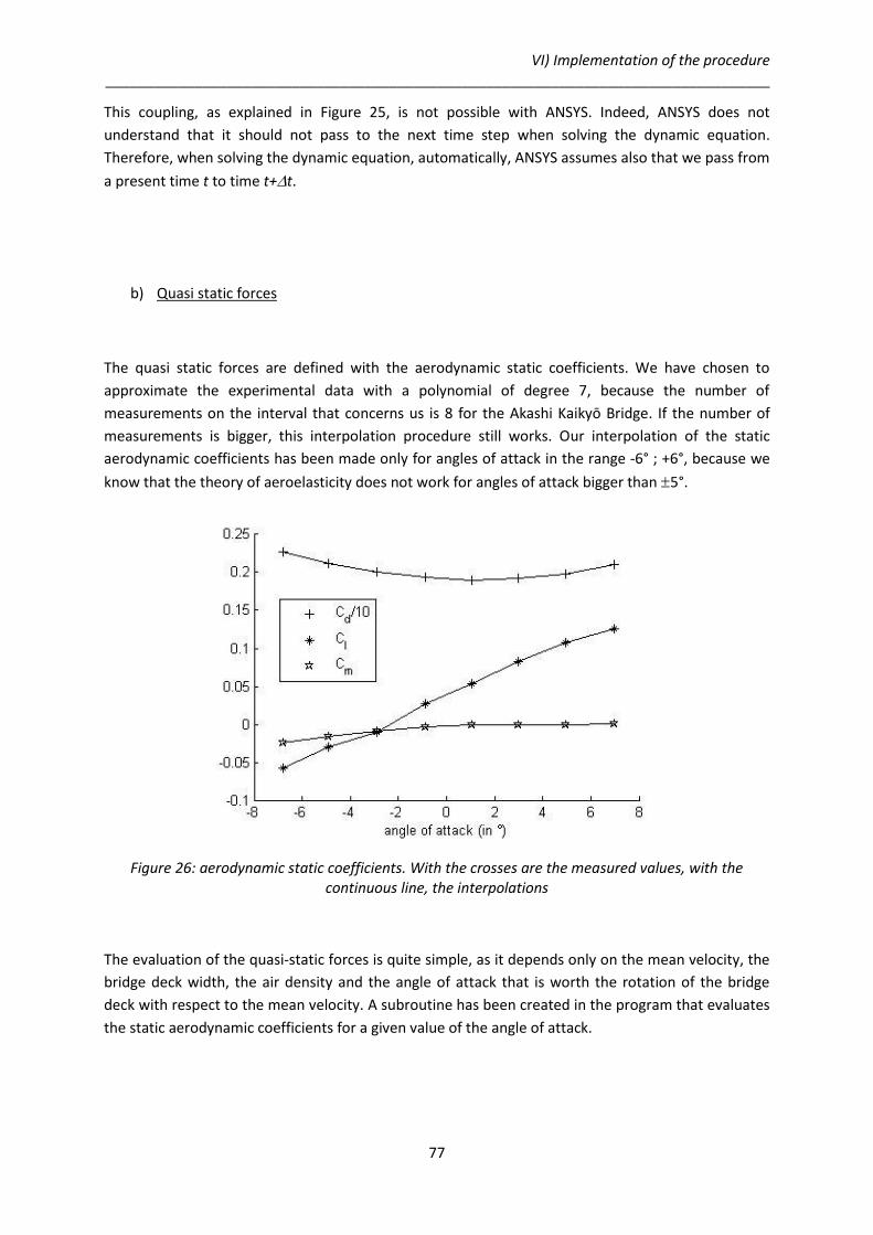
VI) Implementation of the procedure __________________________________________________________________________________
77
This coupling, as explained in Figure 25, is not possible with ANSYS. Indeed, ANSYS does not
understand that it should not pass to the next time step when solving the dynamic equation.
Therefore, when solving the dynamic equation, automatically, ANSYS assumes also that we pass from
a present time t to time t+t.
b) Quasi static forces
The quasi static forces are defined with the aerodynamic static coefficients. We have chosen to
approximate the experimental data with a polynomial of degree 7, because the number of
measurements on the interval that concerns us is 8 for the Akashi Kaikyō Bridge. If the number of
measurements is bigger, this interpolation procedure still works. Our interpolation of the static
aerodynamic coefficients has been made only for angles of attack in the range -6° ; +6°, because we
know that the theory of aeroelasticity does not work for angles of attack bigger than 5°.
Figure 26: aerodynamic static coefficients. With the crosses are the measured values, with the continuous line, the interpolations
The evaluation of the quasi-static forces is quite simple, as it depends only on the mean velocity, the
bridge deck width, the air density and the angle of attack that is worth the rotation of the bridge
deck with respect to the mean velocity. A subroutine has been created in the program that evaluates
the static aerodynamic coefficients for a given value of the angle of attack.

VI) Implementation of the procedure __________________________________________________________________________________
78
c) Self-excited forces and buffeting
As we have seen in V.a), we evaluate the self-excited forces and the buffeting forces together, by
assuming that the vertical gust velocities are added to the vertical motion of the bridge deck. To
evaluate the self-excited and buffeting forces, we have to consider the time history of the bridge
deck through a convolution product of the time-history and of the indicial functions. This convolution
requires an operation of integration. If we consider the case of the lift as a function of the angle of
attack, the expression is:
We know from IV.a), that this integral can be transformed in practice into:
By transforming the integral into a discrete sum and translating the time axis in order that the
present time is worth 0:
Where is defined as the floor function of .
A subroutine evaluates , the value of the indicial function in 0 and another subroutine
evaluates the derivatives of the indicial functions, , for every integration time step, with
the exponential groups formula.
d) Initialization of the time-history input file
As the time-history input file is called in the main program of the module, it has to be initialized. This
operation is realized in another procedure that has to be executed before executing the main
program. This procedure creates the file that contains the time history-motion of the bridge deck and
sets to zero the time-history motion. The files that are created while initializing are called
“angolodatacco.txt” for the angle of attack, “dangolodatacco.txt”, for the derivative of the angle of
attack, “dspostvert.txt”, for the vertical velocity and “d2spostvert.txt”, for the vertical acceleration.
Cf. the 2nd Appendix, paragraph b), to see the procedure coded.

79
3rd Part: Practical applications
VII) Validation of the program
In order to ensure that the program we have realized gives true results, we have to validate it. The
validation procedure that has been adopted is the following one:
- we assume forced harmonic oscillations of the degrees of freedom of the bridge deck section
for a given frequency in input of the program
- we have the program evaluate the wind forces on a time interval worth at least twice the
integration time (sl=20)
- we compare the obtained results with the flutter derivatives for the oscillation frequency
chosen.
a) Validation procedure
The validation procedure we use to control the program is to assume a harmonic motion of the
bridge deck in input of the program and have the program evaluate the self excited forces induced.
Using the program this way is like recreating the wind tunnel experience, by forcing the oscillations
of the bridge deck and measuring the wind forces induced.
In order to create these forced oscillations, the program implemented in VI) has been slightly
modified. We have inserted the procedure initially implemented into a loop on time that generates
the present position of the bridge deck for the different times of the study. In the 2nd Appendix,
paragraph a), the program used for the validation of the procedure has been enclosed. The loop on
the variable J is the loop that we have added.

VII) Validation of the procedure __________________________________________________________________________________
80
1) Forced oscillations of the angle of attack
We assume a unitary harmonic motion of the bridge deck attack angle under the form:
This unitary oscillation is harmonic and function of the dimensionless time, s.
In output of our program, we obtain the following forces, lift, Fz and pitching moment, My:
Figure 27: Input and output of the program for an oscillating angle of attack
To obtain Figure 27, we have fixed the following parameters:
- Aerodynamic coefficients for the indicial functions of the Akashi- Kaikyō Bridge
- reduced frequency:
- dimensionless time path,
- integration time,
- mean wind speed,
- the lift force, FZ is expressed in N/m
- the pitching-moment, My, is expressed in Nm/m
These conditions are the one corresponding with the FORTRAN code in Appendix 2.b).

VII) Validation of the procedure __________________________________________________________________________________
81
After a brief transient time (circa s=2), we note that the induced wind forces are harmonic too, with
the same frequency of oscillation. The phase and the amplitude are different between these two
signals.
In order to compare these results with the expected one, we use the well-known equation by Scanlan
and Simiu [10], considering only the angle of attack:
The angle of attack is worth: or, as a function of dimensional parameters:
, as and .
Therefore,
And so,
Where and
are the interpolated flutter derivatives, as defined in chapter V.d). We use these
values instead of the measured ones, because the indicial functions coefficients are defined on the
basis of the interpolated flutter derivatives.
We can reformulate the lift and pitching moment as a function of an amplitude and phase
differences between both signals:
Where:
- is the lift amplitude defined as:
- is the pitching-moment amplitude defined as:

VII) Validation of the procedure __________________________________________________________________________________
82
- is the lift phase difference defined as:
- is the pitching-moment phase difference defined as:
.
We have to pay a particular attention in the use of the function arg. This function is defined on the
base of the function atan, also called arctan or tan-1 that is the arctangent function. The function arg
is defined as follows:
In the case of the phase difference of the lift, and
. The amplitude and phase
differences are functions of the frequency of oscillation. To validate the program, we have the
program run for a certain number of frequencies of oscillation. Then, we determine the amplitude
and phase differences of the resulting forces in output with respect to the input harmonic signal. And
finally, we compare the amplitude and phase differences of these two pieces of information: they
should be equal.
2) Forced oscillations of the vertical velocity
By doing the same reasoning for the lift and the moment as a function of the vertical motion of the
airfoil, we have the following equations for the vertical motion of the bridge deck and for the lift and
the pitching moment:
VII) Validation of the procedure __________________________________________________________________________________
83
Modifying the expression of the lift and of the moment:
which can also be written under the form of an amplitude coefficient and of a phase difference:
Where:
-
-
-
-
To validate the self-excited wind forces as functions of the vertical velocity of the bridge deck, we
should assume the angle of attack being equal to zero, and create forced oscillations of the vertical
velocity of the bridge deck. Finally, as with the angle of attack, we can just compare both results by
comparing the amplitude and phase differences.
For both of the examples treated below, the parameters of the program have been fixed:
- the dimensionless time path is worth: ds=0.01
- the dimension of the time-history input file is 2000 lines: the integration time is worth sL= 20
b) Akashi Kaikyō Bridge: forced oscillations of the bridge deck
1) Forced oscillations of the angle of attack
Using the formula obtained in VII.a.1), we evaluate what should be the amplitude and phase
differences for the lift as a function of the angle of attack, in theory. Cf. 3rd Appendix, paragraph a),
for the MATLAB code used for the determination of the graphs of amplitude and phase difference.

VII) Validation of the procedure __________________________________________________________________________________
84
Then, using the MATLAB code enclosed in the 3rd Appendix, paragraph b), we can recover the
amplitude and phase differences from the wind forces in output of the FORTRAN procedure.
Figure 28: phase difference and amplitude for the lift as a function of the reduced velocity of oscillation of the angle of attack
Figure 29: phase difference and amplitude for the moment as a function of the reduced velocity of oscillation of the angle of attack
For k=0.2:
From the flutter derivatives
In output of the program
Validated
Amplitude of the lift 1.94 1.97 Yes
Phase difference of the lift -2.74 -2.75 Yes
Amplitude of the moment 0.298 0.265 Yes
Phase difference of the moment
0.095 -0.07 Yes

VII) Validation of the procedure __________________________________________________________________________________
85
For k=0.5:
From the flutter derivatives
In output of the program
Validated
Amplitude of the lift 2.84 2.85 Yes
Phase difference of the lift -2.54 -2.56 Yes
Amplitude of the moment 0.29 0.27 Yes
Phase difference of the moment
-0.27 -0.15 Yes
For k=1:
From the flutter derivatives
In output of the program
Validated
Amplitude of the lift 4.13 4.12 Yes
Phase difference of the lift -2.59 -2.60 Yes
Amplitude of the moment 0.28 0.27 Yes
Phase difference of the moment
-0.27 -0.28 Yes
2) Forced oscillations of the vertical velocity of the bridge deck
Using the formula obtained in VII.a.1), we evaluate what should be the amplitude and phase
differences for the lift as a function of the vertical velocity of the bridge deck, in theory.
Figure 30: phase difference and amplitude for the lift as a function of the reduced velocity of oscillation of the vertical motion

VII) Validation of the procedure __________________________________________________________________________________
86
Figure 31: phase difference and amplitude for the moment as a function of the reduced velocity of oscillation of the vertical motion
For k=0.2:
From the flutter derivatives
In output of the program
Validated
Amplitude of the lift 0.095 0.123 Yes (30% error)
Phase difference of the lift -2.73 -2.88 Yes
Amplitude of the moment 0.017 0.017 Yes
Phase difference of the moment
0 0 Yes
For k=0.5:
From the flutter derivatives
In output of the program
Validated
Amplitude of the lift 0.11 0.138 Yes (30% error)
Phase difference of the lift -2.62 -2.73 Yes
Amplitude of the moment 0.017 0.017 Yes
Phase difference of the moment
0 -0.01 Yes
For k=1:
From the flutter derivatives
In output of the program
Validated
Amplitude of the lift 0.15 0.17 Yes
Phase difference of the lift -2.35 -2.51 Yes
Amplitude of the moment 0.017 0.017 Yes
Phase difference of the moment
0 -0.01 Yes

VII) Validation of the procedure __________________________________________________________________________________
87
c) Tsurumi Bridge: Forced oscillations of the bridge deck
We proceed in the same way to validate the program with the Tsurumi bridge cross-section. First, we
evaluate the amplitude of oscillation and the phase for the lift and the pitching-moment as a function
of the angle of attack and of the vertical velocity of the bridge deck with the interpolated flutter
derivatives. Then we have the program run with forced oscillation for a given set of frequency values
and we evaluate the amplitude and the phase difference of the response. Finally, we compare the
expectable results and the obtained ones.
Figure 32: Flutter derivatives of the Tsurumi bridge deck
Exponential coefficients for the approximation of the indicial functions of the Tsurumi Fairway
Bridge:
Indicial Functions a1 b1 a2 b2 a3 b3
Tsurumi Fairway Lz 3.035 1.316 - - - -
L -1.868 1.978 0.784 0.559 -0.334 0.101
Mz 0.829 0.348 - - - -
M 0.305 0.390 - - - -

VII) Validation of the procedure __________________________________________________________________________________
88
Figure 33: Shape of the four indicial functions of the Tsurumi Fairway Bridge
The other values we need for the evaluation of the self-excited forces are:
- B = 38m
- CL’=-3.370
- CM’=0.943
1) Forced oscillations of the bridge deck attack angle
Figure 34: Amplitude of oscillation and phase difference for the lift for a harmonic angle of attack

VII) Validation of the procedure __________________________________________________________________________________
89
Figure 35: Amplitude of oscillation and phase difference for the pitching moment for a harmonic angle of attack
For k=0.2:
From the flutter derivatives
In output of the program
Validation
Amplitude of the lift 4.04 4.12 Yes
Phase difference of the lift -3.08 -3.07 Yes
Amplitude of the moment 0.89 0.89 Yes
Phase difference of the moment
-0.13 -0.13 Yes
For k=0.5:
From the flutter derivatives
In output of the program
Validation
Amplitude of the lift 3.68 3.74 Yes
Phase difference of the lift -3.03 -3.04 Yes
Amplitude of the moment 0.78 0.78 Yes
Phase difference of the moment
-0.18 -0.19 Yes

VII) Validation of the procedure __________________________________________________________________________________
90
For k=1:
From the flutter derivatives
In output of the program
Validation
Amplitude of the lift 4.07 4.05 Yes
Phase difference of the lift -2.78 -2.76 Yes
Amplitude of the moment 0.70 0.70 Yes
Phase difference of the moment
-0.15 -0.14 Yes
2) Forced oscillations of the bridge deck vertical velocity
Figure 36: Amplitude and phase difference of the lift for a harmonic vertical velocity of the bridge deck
Figure 37: Amplitude and phase difference for the pitching-moment for a harmonic vertical velocity of the bridge deck

VII) Validation of the procedure __________________________________________________________________________________
91
For k=0.2:
From the flutter derivatives
In output of the program
Validation
Amplitude of the lift 0.18 0.18 Yes
Phase difference of the lift 2.69 2.69 Yes
Amplitude of the moment 0.043 0.043 Yes
Phase difference of the moment
-0.42 -0.42 Yes
For k=0.5:
From the flutter derivatives
In output of the program
Validation
Amplitude of the lift 0.21 0.21 Yes
Phase difference of the lift 2.12 2.11 Yes
Amplitude of the moment 0.029 0.029 Yes
Phase difference of the moment
-0.72 -0.73 Yes
For k=1:
From the flutter derivatives
In output of the program
Validation
Amplitude of the lift 0.26 0.26 Yes
Phase difference of the lift 1.50 1.43 Yes
Amplitude of the moment 0.018 0.018 Yes
Phase difference of the moment
-0.78 -0.78 Yes
Conclusion
In the last two paragraphs, we have validated the procedure implemented in VI) by evaluating the
self-excited forces on two cases, the Akashi-Kaikyō Bridge and the Tsurumi Fairway Bridge. The
difference between the results that we expected from the flutter derivatives interpolation and the
results obtained in output of the program is always under 10% of error. The biggest error that is
made is for the pitching-moment as a function of the angle of attack for the Akashi-Kaikyō Bridge. In
this case, the error is of nearly 30%. It is due to the shape of the corresponding indicial function (cf.
Figure 22): the exponential representing the indicial function varies so quickly at the beginning (for s
close to 0) that the time discretization used for integrating the convolution product is probably too
small to give a precise result. In the last paragraph of this chapter, we will test the program, by
changing some variables and see if the evaluated wind forces are more precise and/or converge
better .

VII) Validation of the procedure __________________________________________________________________________________
92
d) Tests on the program
Some parameters of the program have been fixed for the validation process. In this paragraph, we
will see what influence they have on the quality of the results. The parameters that have been fixed
are the integration time path of the convolution product, ds, and the integration time, sL. In order to
better understand their influence, we will always study the same case in this paragraph: the moment
a function of the angle of attack for the Akashi Kaikyō Bridge at a frequency of oscillation of the angle
of attack worth k = 0.5.
1) Influence of the dimensionless time path
This parameter has been fixed at 0.01 for the previous validation process. To test its importance, we
have fixed it at three different values, 1, 0.1 and 0.01. The integration time is worth sL=20.
Figure 38: influence of the integration time path, ds
When the dimensionless time path is reduced, the results get more accurate. It seems that in this
case, a time path worth ds=0.1 is sufficient to have a good evaluation of the lift. By reducing the time
path, we increase the precision of the results but we also increase the run time of the program.
Indeed, in our program, because of the reading and re-writing of the time-history motion at each
time step, dividing the time step by 10 is like increasing the run time of the program by 100.

VII) Validation of the procedure __________________________________________________________________________________
93
Normally, the time step is not set up by the user; it is set up by the computing framework that
executes the module. The time step is a piece of data that is fixed when solving the dynamic
equation. Anyway, when we use this module, we have to take care that the dimensionless time path
is not smaller than 0.1. If it is smaller than this value, it means that the time step should be reduced
for the need of the module.
2) Influence of the integration time, sL
The integration time is the time defined in IV.a):
The integration time is the time interval on which we have to integrate the convolution product. It
corresponds to the time-history interval that we have to consider to evaluate the present wind
forces. To evaluate its influence, as done in VII.d.1), we will consider different values of the
integration time: 1, 5 and 20. The integration time path is fixed at 0.1, as we have seen previously
that it is small enough.
Figure 39: influence of the integration time, sL
In the article [15], it is said that an integration time that should always be big enough is sL worth 10. It
is verified in our case, as for sL=2, we already nearly have convergence.
94
Conclusions
The present work has been developed along three lines: 1) the theoretical background required to
understand and formulate the wind forces expressed through indicial functions, 2) the
implementation of a computer procedure for the evaluation of said wind forces and, finally, 3) the
validation of that procedure.
The theoretical part developed in this thesis resumes different approaches to the indicial functions
derivations, some of them pursued in literature and some other newly formulated, showing their
substantial equivalence from the point of view of the results. This part is of paramount importance in
order to correctly formulate the problem and understand the limits of the theories adopted.
In the implementation part, a particular attention has been made with regards to the future use of
code developed. This has been implemented as a FORTRAN90 module that has to be called from a
bigger computing structure, such as a finite element software or, in this initial cases a smaller,
independent, driver program. The program that has been implemented works for one cross-section
of a bridge deck. It has been tested and validated on the Akashi-Kaikyō Bridge and the Tsurumi
Fairway Bridge cases, by studying the self-excited component of the wind forces.
Further work is needed on the subject of indicial functions applied to bridges, not only from the
theoretical point of the validity of the linearity hypothesis but also for the mundane implementation
part. The procedure here developed, that has been used only on one cross-section, can easily be
extended to a whole bridge span. In this case, in several sections along the bridge deck the wind
forces can be independently evaluated. The procedure can easily be modified so that it can be called
within a main ANSYS data file, by means of APDL interface routines, and its result can be
reintroduced in the ANSYS structural case in the form of external nodal forces. This allows for the
evaluation of the dynamic behavior of a whole bridge without requiring the cumbersome
development of a specific ANSYS aerodynamic element. This would help understanding better the
possible phenomenon of flutter from the point of view of the whole bridge, and not only of a bridge
deck cross-section.
Finally, the buffeting component of the wind forces may be also further developed; from the
theoretical point view, by trying to obtain the Küssner’s type indicial functions for a bridge deck
cross-section, and also from the practical point view of its implementation.

95
1st Appendix: Fourier analysis, definition and properties
a) Introduction to the Fourier transform We assume that we are in the aeroelastic conditions. Therefore, the wind forces are linked linearly to
the motion of the bridge deck for harmonic oscillations, through the flutter derivatives which are
function of the frequency of oscillation of the airfoil. Using the typical notation for a Fourier
transform analysis, we will call Z(iω), the complex impedance, function of the pulsation of oscillation,
ω, that links proportionally the motion and the wind forces.
If the forced function F(t) is harmonic: tieFtF
0)(
Using the linearity of the problem, we obtain a response, y(t), which is harmonic too and at the same
pulsation:
)(
)()(
iZ
tFty
If the forced function is a sum of harmonic motions, using the superposition principle that
corresponds with the linearity of the studied problem:
tin
n
neCtF
)(
n
tinn einZ
Cty
)()(
For a non periodic function, we use the Fourier transform, to transform our forced function into an
integral depending on the frequencies of oscillation:
dtetFG ti
)(2
1)(
deGtF ti
)(2
1)(
)(G is the Fourier transform of F. And F’ is the inverse Fourier transform of )(G .
It can be demonstrated that if the function F(t) is smooth enough, the inverse Fourier transform of
the Fourier transform is equal to the function itself, and therefore that F’(t)=F(t). Cf. [22] for details
on the demonstration. For a physical case, as ours, we will assume that this property is always
verified.

96
Using the impedance Z, we know that the response to the forced function F is equal to the inverse
Fourier transform of G(ω) multiplied by the complex impedance, so:
deiZ
Gty ti
)(
)(
2
1)(
b) Response to an impulse
If we consider as the forced function, a step-function,
This function is also called Heaviside function. It corresponds to a unitary abrupt change of the value
of the forced function.
The derivative of such a function is the Dirac distribution, :
Where means a derivate with respect to time.
If the abrupt change happens at time τ different from t=0:
The Dirac distribution can be seen as a function equal to zero along all the axis of real numbers,
except on the interval , such as:
This means that even if tends to an infinite value for t=0, its integral remains convergent and
equal to one.

97
We look for the response to such an impulse happening at a time τ, considering our system still linear
and invariable in time. If we know the complex impedance of our system, Z(iω), we first calculate the
Fourier transform of the Dirac :
dtetG ti
)(2
1)(
ieG
2
1)(
Assuming that the Dirac function is still smooth enough to do the reasoning we have done before,
we obtain, that the Fourier inverse transform response to the Dirac function is equal to:
deiZ
Gty ti
)(
)(
2
1)(
deiZ
ty ti )(
)(
1
2
1)(
Ths function is equal to the Fourier transform of the inverse of the complex impedance, with a
translation on the time axis. We evaluate it not at t but at the time t-τ.

98
2nd Appendix: Implemented code in FORTRAN
The present code is the code used for the validation of the procedure. This case corresponds with the case k=0.2, sL=20 and ds=0.1, for evaluating the lift and pitching-moment corresponding to a harmonic oscillation of the bridge deck, as done in VII.a). To learn how to code in FORTRAN90, I have consulted references [23] and [24].
The main program is presented first. Further on, is also presented the initialization code.
a) Main program program forzefunzindiciali implicit none double precision,dimension(4) :: X ! vettore posizione (3 spost (x,y,z) + una rot) double precision :: L=1.0 ! lunghezza d'influenza del nodo double precision :: Umed=20.0 ! velocità media del vento orrizontale lungo x double precision :: ro=1.2 ! densità aria double precision :: B ! B maiuscolo, dim dell'impalcato di ponte double precision,dimension(4) :: v_nodo ! vettore velocità del nodo (3 spost + una rot) double precision,dimension(3) :: vflut_nodo ! vettore fluttazione velocità vento al nodo (wind gusts) double precision,dimension(4,5) :: coeff_funz ! array with the coefficients ai and bi of the indicial funtions. ! 1st number: function, 2nd number: coefficients a0,a1,a2,b1,b2 double precision :: dCl,dCm ! derivatives of the lift and pitching moment with respect to the angle of attack in 0 double precision :: ds=0.01 ! passo temporale double precision :: t,s ! time and dimensionless time double precision :: coeffmultipL ! coeff multiplicativo davanti all'integrale nella formulazione di Jones per il lift double precision :: coeffmultipM ! coeff multiplicativo davanti all'integrale nella formulazione di Jones per il momento integer :: N=2000,M=5000 ! N is number of time-history position we keep in memory ! M is the number of iteration done in the validation phase double precision, dimension(1000) :: alpha ! storia angolo d'attaco double precision, dimension(1000) :: dalpha ! storia deriv angolo d'attaco double precision, dimension(1000) :: dh ! storia deriv spost verticale double precision, dimension(1000) :: ddh ! storia deriv seconda spost verticale double precision,dimension(3,7000) :: Fe ! Fe(1): Fx. Fe(2): Fz. Fe(3): My ! variabili locali double precision :: Fd=0d0 double precision :: Fl=0d0 double precision :: Fm=0d0 double precision :: Cd double precision :: Cl double precision :: Cm double precision :: modulo double precision :: pLh,pLalpha,pMh,pMalpha integer :: I,J

99
! variabili locali per forze aerodinamiche linearizzate double precision :: gamma_r,attack_angle double precision :: k=0.2 do J=1,M,1 ! we create a loop inside the program only for the validation phase open(34,file='alpha.txt') ! File dove viene scritto l’angolo d’attaco instantaneo open(35,file='dalpha.txt') ! File dove viene scritto la derivate dell’angolo d’attaco instantaneo open(36,file='dh.txt') ! File dove viene scritte la velocità verticale instantanea open(37,file='ddh.txt') ! File dove viene scritto l’accelerazione verticale instantanea write(34,*) cos(k*J*ds) ! Imponiamo un moto armonico all’angolo d’attaco write(35,*) –k*sin(k*J*ds) write(36,*) 0.000 ! moto vertical bloccato write(37,*) 0.000 close(34) close(35) close(36) close(37) v_nodo(:)=0d0 vflut_nodo(:)=0d0 X(:)=0d0 coeff_funz(:,:)=1.0 !-----Azzeramento variabili Fe(:,J)=0d0 Fd=0d0 Fl=0d0 Fm=0d0 Cd=1.0 Cl=0d0 Cm=0d0 gamma_r=0d0 modulo=0d0 open(20,file='Coefficientsfunzioniindiciali.txt') !lettura dati sulle funzioni indiciali read(20,*) read(20,*) read(20,*) (coeff_funz(1,I),I=2,5) read(20,*) read(20,*) (coeff_funz(2,I),I=2,5) read(20,*) read(20,*) (coeff_funz(3,I),I=2,5) read(20,*) read(20,*) (coeff_funz(4,I),I=2,5) read(20,*) read(20,*) read(20,*) B read(20,*) read(20,*) dCl read(20,*) read(20,*) dCm close(20) coeffmultipL=0.5*ro*B*Umed*Umed*dCl coeffmultipM=0.5*ro*B*B*Umed*Umed*dCm if(ds*N<10) print*, "error: integration time, sL, too short" ! the integration time is worth N*ds, the number of position
! kept in memory multiplied by the dimensionless time step

100
open (30, file='angolodatacco.txt') open (31, file='dangolodatacco.txt') open (32, file='dspostvert.txt') open (33, file='d2spostvert.txt') ! lettura della time-history motion dell’impalcato di ponte, nei file di input do I=2,N,1 read(30,*) alpha(I) read(31,*) dalpha(I) read(32,*) dh(I) read(33,*) ddh(I) end do close(30) close(31) close(32) close(33) ! lettura della posizione attuale dell’impalcato di ponte. Quest’informazione può provenire da ANSYS. In questo caso, viene ! definita da noi ad ogni instante. open(34,file='alpha.txt') open(35,file='dalpha.txt') open(36,file='dh.txt') open(37,file='ddh.txt') read(34,*) alpha(1) read(35,*) dalpha(1) read(36,*) dh(1) read(37,*) ddh(1) close(34) close(35) close(36) close(37) attack_angle=alpha(1) ! Calcoliamo le forze del vento su un nodo corrispondente ad una lunghezza L ! Calcolo modulo del vettore Vr modulo=(Umed+(vflut_nodo(1)-v_nodo(1)))**2+(vflut_nodo(3)-v_nodo(3))**2 !--------Calcola Cd, Cl e Cm in funzione dell'angolo di attacco ! Calcolo angolo tra Vr ed asse di riferimento solidale con la sezione, in radianti gamma_r=atan((vflut_nodo(3)-v_nodo(3))/(Umed+(vflut_nodo(1)-v_nodo(1)))) ! attack_angle=gamma_r+X(4) ! Calcolo il Cd ed il Cl dato l'angolo di attacco in radianti ! call evaluate_CdClCm(attack_angle,Cd,Cl,Cm) ! Calcolo forze di drag e di lift ! Fd=0.5*ro*modulo*B*Cd ! Non calcoliamo le forze quasi-statiche, vogliamo solo le self-excited forces ! Fl=0.5*ro*modulo*B*Cl ! Fm=0.5*ro*modulo*B*B*Cm t=0d0 s=0d0 call evaluatePhi(coeff_funz,t,pLh,pLalpha,pMh,pMalpha) ! Valutazione della funzione indiciale in 0 Fl=Fl+coeffmultipL*(pLalpha*alpha(1)+pLh*dh(1)*2/B) ! calcolo della costante presente nell’espression delle !
self-excited forces Fm=Fm+coeffmultipM*(pMalpha*alpha(1)+pMh*dh(1)*2/B)

101
s=-N*ds; do I=1,N,1 ! Valutazione della funzione indiciale al tempo -sigma call evaluatedPhi(coeff_funz,-s,pLh,pLalpha,pMh,pMalpha) Fl=Fl+coeffmultipL*(pLalpha*alpha(N+1-I)+pLh*dh(N+1-I)*2/B)*ds ! Calcolo del prodotto di convoluzione discretizzato Fm=Fm+coeffmultipM*(pMalpha*alpha(N+1-I)+pMh*dh(N+1-I)*2/B)*ds s=s+ds end do ! rotazione per ricavare le forze lungo (0x), (Oz) e il momento attorno a (Oy), ! con angolo pari all'angolo d'attacco. NON NECESSARIO NEL NOSTRO CASO !Fe(1,J)=L*(Fd*cos(attack_angle)-Fl*sin(attack_angle)) !Fe(2,J)=L*(Fd*sin(attack_angle)+Fl*cos(attack_angle)) !Fe(3,J)=L*Fm Fe(1,J)=L*Fd Fe(2,J)=L*Fl Fe(3,J)=L*Fm open (30, file='angolodatacco.txt') open (31, file='dangolodatacco.txt') open (32, file='dspostvert.txt') open (33, file='d2spostvert.txt') ! Update del file di time-history motion do I=1,N,1 write(30,*) alpha(I) write(31,*) dalpha(I) write(32,*) dh(I) write(33,*) ddh(I) end do close(30) close(31) close(32) close(33) end do ! Fine del ciclo di modelazione delle oscillazione armoniche forzate ! Scrittura delle forze in output open(100,file='resultFe.txt') do J=1,M,1 write(100,*) Fe(:,J) end do close(100) end program forzefunzindiciali ! Valutazione dei coefficient aerodinamici statici per un certo valore dell’angolo d’attaco subroutine evaluate_CdClCm(attack_angle,Cd,Cl,Cm) implicit none double precision, intent(IN):: attack_angle double precision, intent(OUT):: Cd,Cl,Cm ! variables locales double precision, dimension(8):: coeffCd, coeffCl, coeffCm

102
integer:: i=1 ! lettura del file di input con i dati dei coefficienti aerodinamici statici open(10,file='CdClCmcoeffs.txt') read(10,*) read(10,*) coeffCd(:) read(10,*) read(10,*) read(10,*) coeffCl(:) read(10,*) read(10,*) read(10,*) coeffCm(:) close(10) ! !!!! Metodo di calcolo dei coefficienti aerodinamici valido solo per angoli compresi fra -6° e +6° Cd=0d0 Cl=0d0 Cm=0d0 if (abs(attack_angle)<0.00001)then Cd=coeffCd(1) Cl=coeffCl(1) Cm=coeffCm(1) else do i=1,8,1 Cd=Cd+coeffCd(i)*attack_angle**(i-1) Cl=Cl+coeffCl(i)*attack_angle**(i-1) Cm=Cm+coeffCm(i)*attack_angle**(i-1) end do endif endsubroutine subroutine evaluatedPhi(coeff_funz,s,pLh,pLalpha,pMh,pMalpha) implicit none double precision,dimension(4,5), intent(IN):: coeff_funz double precision, intent(IN) :: s double precision, intent(OUT) :: pLh,pLalpha,pMh,pMalpha pLh=coeff_funz(1,3)*coeff_funz(1,2)*exp(-coeff_funz(1,3)*s)+coeff_funz(1,4)*coeff_funz(1,5)*exp(-coeff_funz(1,5)*s) pLalpha=coeff_funz(2,3)*coeff_funz(2,2)*exp(-coeff_funz(2,3)*s)+coeff_funz(2,4)*coeff_funz(2,5)*exp(-coeff_funz(2,5)*s) pMh=coeff_funz(3,3)*coeff_funz(3,2)*exp(-coeff_funz(3,3)*s)+coeff_funz(3,4)*coeff_funz(3,5)*exp(-coeff_funz(3,5)*s) pMalpha=coeff_funz(4,3)*coeff_funz(4,2)*exp(-coeff_funz(4,3)*s)+coeff_funz(4,4)*coeff_funz(4,5)*exp(-coeff_funz(4,5)*s) endsubroutine subroutine evaluatePhi(coeff_funz,s,pLh,pLalpha,pMh,pMalpha) implicit none double precision,dimension(4,5), intent(IN):: coeff_funz double precision, intent(IN) :: s double precision, intent(OUT) :: pLh,pLalpha,pMh,pMalpha pLh=coeff_funz(1,1)-coeff_funz(1,2)*exp(coeff_funz(1,3)*s)-coeff_funz(1,4)*exp(coeff_funz(1,5)*s) pLalpha=coeff_funz(2,1)-coeff_funz(2,2)*exp(coeff_funz(2,3)*s)-coeff_funz(2,4)*exp(coeff_funz(2,5)*s) pMh=coeff_funz(3,1)-coeff_funz(3,2)*exp(coeff_funz(3,3)*s)-coeff_funz(3,4)*exp(coeff_funz(3,5)*s) pMalpha=coeff_funz(4,1)-coeff_funz(4,2)*exp(coeff_funz(4,3)*s)-coeff_funz(4,4)*exp(coeff_funz(4,5)*s) endsubroutine

103
b) Initialization program program ini implicit none integer :: I integer :: N=2000 open(10,file='angolodatacco.txt') open(11,file='dangolodatacco.txt') open(12,file='dspostvert.txt') open(13,file='d2spostvert.txt') do I=1,N,1 write(10,*) 0d0 write(11,*) 0d0 write(12,*) 0d0 write(13,*) 0d0 end do end program ini

104
3rd Appendix: MATLAB code for the validation of the procedure
a) Code for the evaluation of amplitude and phase differences using the flutter derivatives
k=[0.10:0.01:1.2];
% aerodynamic coefficients of the Akashi Kaikyō Bridge deck
dCl=-1.192;
dCm=0.307;
B=35.5;
aLh=[1;-0.365;-11.652];
bLh=[0.021;7.235];
aLa=[1;-0.392;-3.653];
bLa=[0.008;1.155];
aMh=[1;0.039;0.0];
bMh=[0.0;0.0];
aMa=[1;0.073;1.758];
bMa=[0.025;7.098];
% Evaluation of the flutter derivatives interpolated with the coefficients of the
% indicial functions.
H1approx=dCl./(2*k).*((aLh(1)-aLh(2)-
aLh(3))+(aLh(2)*bLh(1)^2./(k.^2+bLh(1)^2))+(aLh(3)*bLh(2)^2./(k.^2+bLh(2)^2)));
H4approx=dCl/2*(aLh(2)*bLh(1)./(k.^2+bLh(1)^2)+aLh(3)*bLh(2)./(k.^2+bLh(2)^2));
H3approx=dCl./((2*k).^2).*((aLa(1)-aLa(2)-
aLa(3))+(aLa(2)*bLa(1)^2./(k.^2+bLa(1)^2))+(aLa(3)*bLa(2)^2./(k.^2+bLa(2)^2)));
H2approx=-dCl./(4*k).*(aLa(2)*bLa(1)./(k.^2+bLa(1)^2)+aLa(3)*bLa(2)./(k.^2+bLa(2)^2));
A1approx=dCm./(2*k).*((aMh(1)-aMh(2)-
aMh(3))+(aMh(2)*bMh(1)^2./(k.^2+bMh(1)^2))+(aMh(3)*bMh(2)^2./(k.^2+bMh(2)^2)));
A4approx=dCm./(2*k).*(aMh(2)*bMh(1)./(k.^2+bMh(1)^2)+aMh(3)*bMh(2)./(k.^2+bMh(2)^2)
);
A3approx=dCm./((2*k).^2).*((aMa(1)-aMa(2)-
aMa(3))+(aMa(2)*bMa(1)^2./(k.^2+bMa(1)^2))+(aMa(3)*bMa(2)^2./(k.^2+bMa(2)^2)));
A2approx=dCm./((2*k).^2).*((aMa(2)*bMa(1)./(k.^2+bMa(1)^2)+aMa(3)*bMa(2)./(k.^2+bMa
(2)^2)));
% evaluation of the amplitude differences
AMPLa=4*k.^2.*sqrt(H2approx.^2+H3approx.^2);
AMPLh=4*k.*sqrt(H1approx.^2+H4approx.^2)/B;
AMPMa=4*k.^2.*sqrt(A3approx.^2+A2approx.^2);
AMPMh=4*k.*sqrt(A1approx.^2+A4approx.^2)/B;
% evaluation of the phase differences
if (H3approx(30)>0)
PHASELa=atan(H2approx./H3approx);
else
if (H3approx(30)<0)
if (H2approx(30)>=0)
PHASELa=pi+atan(H2approx./H3approx);

105
else
PHASELa=-pi+atan(H2approx./H3approx);
end
else
if (H2approx(30)>0)
PHASELa=pi*ones(1,length(k));
else
PHASELa=-pi*ones(1,length(k));
end
end
end
if (H4approx(30)>0)
PHASELh=atan(H1approx./H4approx);
else
if (H4approx(30)<0)
if (H1approx(30)>=0)
PHASELh=pi+atan(H1approx./H4approx);
else
PHASELh=-pi+atan(H1approx./H4approx);
end
else
if (H1approx(30)>0)
PHASELh=pi*ones(1,length(k));
else
PHASELh=-pi*ones(1,length(k));
end
end
end
if (A3approx(30)>0)
PHASEMa=atan(-A2approx./A3approx);
else
if (A3approx(30)<0)
if (A2approx(30)>=0)
PHASEMa=pi+atan(-A2approx./A3approx);
else
PHASEMa=-pi+atan(-A2approx./A3approx);
end
else
if (A2approx(30)>0)
PHASEMa=pi*ones(1,length(k));
else
PHASEMa=-pi*ones(1,length(k));
end
end
end
if (A4approx(30)>0)
PHASEMh=atan(A1approx./A4approx);
else
if (A4approx(30)<0)
if (A1approx(30)>=0)
PHASEMh=pi+atan(A1approx./A4approx);
else
PHASEMh=-pi+atan(A1approx./A4approx);
end
else
if (A1approx(30)>0)
PHASEMh=pi*ones(1,length(k));
else
PHASEMh=-pi*ones(1,length(k));
end
end
end

106
figure('color','w')
subplot(1,2,1)
plot(1./k(1:90),PHASELa(1:90),'k')
grid on
title('phase difference')
xlabel('2/K')
subplot(1,2,2)
plot(1./k(1:90), AMPLa(1:90),'k')
grid on
xlabel('2/K')
title('amplitude')
figure('color','w')
subplot(1,2,1)
plot(1./k(1:90),PHASEMa(1:90),'k')
grid on
title('phase difference')
xlabel('2/K')
subplot(1,2,2)
plot(1./k(1:90), AMPMa(1:90),'k')
grid on
xlabel('2/K')
title('amplitude')
figure('color','w')
subplot(1,2,1)
plot(1./k(1:90),PHASELh(1:90),'k')
grid on
title('phase difference')
xlabel('2/K')
subplot(1,2,2)
plot(1./k(1:90), AMPLh(1:90),'k')
grid on
xlabel('2/K')
title('amplitude')
figure('color','w')
subplot(1,2,1)
plot(1./k(1:90),PHASEMh(1:90),'*k')
grid on
title('phase difference')
xlabel('2/K')
subplot(1,2,2)
plot(1./k(1:90), AMPMh(1:90),'*k')
grid on
xlabel('2/K')
title('amplitude')
I=11;
k(I) % I is the position of the studied frequency in the vector k. In this
% case, we are studying the frequency k=0.2
% values of the amplitude and phase differences for k=0.2
AMPLalpha=AMPLa(I)
AMPLspost=AMPLh(I)
AMPMalpha=AMPMa(I)
AMPMspost=AMPLh(I)
PHASELalpha=PHASELa(I)
PHASELspost=PHASELh(I)
PHASEMalpha=PHASEMa(I)
PHASEMspost=PHASELh(I)

107
b) Code developed to obtain the amplitude and phase differences of the wind forces in output
of the program
k=0.2;
B=35.5;
U=20;
ds=0.01;
% resultFe is the output file of our program in which are stored the wind
% forces
WForces=resultFe(1500:end,:); % we do not consider the beginning of the wind forces
% to avoid studying the transient time
lift=WForces(:,2);
moment=WForces(:,3);
[aL,bL]=max(lift);
[aM,bM]=max(moment);
AMPL=aL/(0.5*1.2*B*U^2) % amplitude of the lift
AMPM=aM/(0.5*1.2*B^2*U^2) % amplitude of the moment
DSL=-(bL+1500)*ds;
phiL=k*DSL;
while (phiL<-pi)
phiL=phiL+2*pi;
end
phiL % phase difference for the lift
DSM=-(bM+1500)*ds;
phiM=k*DSM;
while (phiM<-pi)
phiM=phiM+2*pi;
end
phiM % phase difference for the moment

108
4th Appendix: Notations
Froude number
1(t) Heaviside function, also called step function
e Reynolds number
A i# torsional flutter derivative, as expressed by Fung (theoretical)
A i* torsional flutter derivative, as expressed by Scanlan (experimental)
c speed of sound in atmospheric conditions
c chord of the airfoil
C D , C L , C M aerodynamic static coefficients for drag and lift and pitching moment
C L ', C M ' derivate of the static aerodynamic coefficients with respect to in 0
C X , C Z , C M aerodynamic static coefficients for horizontal, vertical forces and pitching moment
D, L drag and lift forces
div divergence operator: div( U )=(∂U x )/∂x+(∂Uy)/∂y+(∂Uz)/∂z
indicial response function for a bridge deck (determined experimentally)
F x , F z , M y horizontal and vertical wind forces and pitching-moment
H i# vertical flutter derivative, as expressed by Fung (theoretical)
H i* vertical flutter derivative, as expressed by Scanlan (experimental)
indicial response function for a thin-airfoil (Wagner)
K dimensionless pulsation also called reduced velocity, Bω/U
k reduced velocity as defined by Theodorsen, k=K/2
M Mach number
dynamic viscosity
M 0 or M a pitching moment
gradient operator:
F=(∂F/∂x; ∂F/∂y; ∂F/∂z)
p relative pressure
P absolute pressure
P 0 air pressure at rest
air density (1,2 kg/m3 in atmospheric condiditons)
rot rotational operator: rot A = (∂A z /∂y-∂A y/∂z; ∂A x/∂z-∂A z /∂x; ∂A y/∂x-∂A x/∂y)
s dimensionless present time, 2Ut/B
s L integration time for the convolution integral
dimensionless time, integration variable
t present time

109

110
Bibliography
1. Darrozes, Jean-Sylvestre and François, Claude. Mécanique des fluides incompressibles. s.l. :
Lecture notes of the lesson MF101 dispensed at ENSTA.
2. Cadot, Olivier. Introduction à la turbulence. s.l. : Lecture notes of the course MF205 dispensed at
ENSTA.
3. Monier, Jean-Marie. Analyse PC-PSI-PT Cours, méthodes et exercices corrigés. s.l. : J'intègre,
Dunod, 2006.
4. Martinelli, Luca and Perotti, Federico. Numerical analysis of the non-linear dynamic behavior of
suspended cables under turbulent excitation. s.l. : International Journal of Structural Stability and
Dynamics, 2001.
5. Howard C. Curtiss Jr., Robert H. Scanlan and Fernando Sisto. A Modern Course in Aeroelasticity.
s.l. : Earl H. Dowell, 1989.
6. Fung, Y. C. An Introdution to the Theory of Aeroelasticity. s.l. : Dover, 1955.
7. Hémon, Pascal. Vibrations des structures couplées avec le vent. s.l. : Les Editions de l'école
Polytechnique, 2006.
8. Kitagawa, Makoto. Technology of the Akashi Kaikyo Bridge. s.l. : Structural Control and Health
Monitoring, 2004.
9. Simiu, E and Scanlan, R. H. Wind Effects on structures, 1st edition. s.l. : John Wiley and Sons, 1978.
10. Simiu, E. and Scanlan, R.H. Wind Effects on Structures, 3rd edition. s.l. : John Wiley & Sons, 1996.
11. Piperno, Serge. Numerical simulation of aeroelastic instabilities of elementary bridge decks. s.l. :
Research Report of the INRIA (Institut National de Recherche en Informatique et en Automatique),
November 1998.
12. Bourquin, Frédéric. (Interview with). Director of the metrology and instrumentation department
of the LCPC (Laboratoire central des Ponts et Chaussées) June 2010.
13. Scanlan, R. H. Motion-Related Body-force functions in a two-dimensional low-speed flow. s.l. :
Journal of Fluids and Structures, 2000.
14. C. Costa, C. Borri, O. Flamand and G. Grillaud. Time-domain buffeting simulations for wind-bridge
interaction. s.l. : Journal of Wind Engineering an Industrial Dynamics, 2007.
15. Borri, C., Costa, C. et Zahlten, W. Non-stationary flow forces for the numerical simulation of
aeroelastic instability of bridge decks. s.l. : Computers and Structures, 2002.
16. Borri, Claudio and Höffer, Rüdiger. Aeroelastic Wind Forces on Flexible Bridge Girders. s.l. :
Meccanica, Kluwer Academic Publishers, 2000.
111
17. Perotti, Prof. F. Studio della risposta di sistemi ad un grado di libertà. s.l. : Lecture notes of the
course "Dinamica delle Stutture" dispensed at Politecnico di Milano.
18. Narui, Shin. Wind tunnel test of Naboky-Bisan-Seto Bridges with stiffening truss.
19. Katsuchi, H., et al. Multi-mode flutter and buffeting analysis of the Akashi-Kaikyo bridge. s.l. :
Journal of Wind Engineering and Industrial Aerodynamics, 1998.
20. Caracoglia, L. et Jones, N. P. Time domain vs. frequency domain characterization of aeroelastic
forces for bridge deck sections. s.l. : Journal of Wind Engineering and Industrial Aerodynamics, 2003.
21. Cazzaniga, Emanuela Noemi. Lecture notes of the course "Trattamento delle osservazioni". s.l. :
lecture at Politecnico di Milano.
22. Laamri, El Haj. Mesures, intégration, convolution et transformée de Fourier des fonctions. s.l. :
Dunod, 2007.
23. Smith, I. M. Programming in Fortran 90 "a first course for Engineers and Scientists". s.l. : John
Wiley and Sons, 1995.
24. Biondini, F. Lecture notes of "Calcolo automatico delle strutture 1". s.l. : Lecture at Politecnico di
Milano.
25. Chen, Z. Q., et al. Investigation on influence factors of buffeting response of bridges and its
aeroelastic model verification for Xiaoguan Bridge. s.l. : Engineering Structures, 2009.


![Mathematical modelling of forces acting on ships during ...Mathematical modelling of forces acting on ships during lightering operations Evert Latairea,n, ... Nomenclature B [m]](https://img.pdfslide.us/doc/110x75/5a934e9f7f8b9a8b5d8c3077/mathematical-modelling-of-forces-acting-on-ships-during-mathematical-modelling.jpg)