IEEE TRANSACTIONS ON EDUCATION. VOL. 38, NO. 4. NOVEMBER 199.5

Integrator 1

317

Integrator 2 output

Time Domain Analysis of Linear Systems Using Spreadsheets

Ali El-Hajj and Karim Y. Kabalan

Abstract-In this paper, a method for the analysis of linear systems using spreadsheets is presented. This method is based on a spreadsheet pictorial simulation of the mathematical per- formance of an integrator. At first, a connecting method, using integrators, is used to symbolize different blocks of the system each representing a given transfer function. These blocks are then c o ~ e c t e d according to the signal flow and the interrelationship existing between them. As a result, the output of the system in response to any given input and any given configuration is evaluated. This method is characterized by its low cost, flexibility, and simplicity.

I. INTRODUCTION

PREADSHEETS have been recently used as an edu- S cational tool in many electrical engineering problems [1]-[5]. In some recent works, spreadsheets were applied as simulation tools for circuits applications [3], simulation of logic networks [4], and for linear circuit analysis [5]. In this work, a novel approach is introduced to simulate a linear system represented by its block diagram, and to calculate its time response to any input signal.

The basic building-block device of this work is the integra- tor. This integrator is represented by a box labeled with its name showing the input, the initial condition, and the output. The mathematical integration is performed using an integration rule [6]. Two integrators are connected in cascade when the input of the second one is assigned a formula equal to the output address of the first integrator. Any transfer function in the s-domain can be simulated by connecting a number of integrators with appropriate scaling coefficients. The overall system is obtained by connecting in the same way individual transfer functions.

To illustrate the method, this paper is divided into four sections. The iterations counter and the integrator simulation are presented in Section 11, and the transfer function and block diagram simulation are presented in Section 111. This method is discussed in Section IV and conclusive remarks are given in Section V.

11. BASIC DEVICES SIMULATION The basic elements used in this simulation are the iteration

counter and the integrator. Row 1 in Fig. 1 shows the spread- sheet simulation of the iteration counter. Counting is achieved

Manuscript received May 18, 1993; revised March 28, 1994. This work was supported by the Research Board of the American University of Beirut.

The authors are with the Electrical Engineering Department, Faculty of Engineering and Architecture, American University of Beirut, Lebanon.

IEEE Log Number 9413578.

A B C D E F G H I J K 1 ICOUNT 0 FLAG : 0 2 STEP: 0.02 3 TIME: 0 4 5 0 6 7 0 - I I - 0 8 I INTEG. I 9 lo

_ _ _ I _ _ _ _ _ _

I , , I _-_------- Fig. 1. Spreadsheet simulation of the counter and integrator.

Fig. 2. Representation of G(s) with adders and integrators.

at cell B1. Cell B1 is initialized to zero and incremented by one at each spreadsheet recalculation. A flag at address F1 is used to reset the counter to zero and the spreadsheet to the initial state. The formula at cell B1 is given by

@IF ($F$I=O, 0 , B l + l ) . (1)

The time value is displayed at cell B3 and obtained by multi- plying the value of the counter (cell B l ) with the integration step size (cell B2).

Fig. 1 also shows the integrator represented by a box whose input is at cell E7 and output is at cell K7. Cell G5 is used to store the initial value existing at the input before any new input signal is applied. This value is used in the integration during the first iteration.

For convenience in the display, the width of the spreadsheet columns is adjusted to accommodate a maximum of three characters per column. The recalculation mode has been set to “rowwise” which allows the placement of many integrators of a complex network on one row and by filling successive rows in the order of propagation of the signal. The integrator uses an integration formula to calculate its output. Simpson’s 1/3 rule [6] has been selected but other formulas can be used as later outlined in Section IV. In this case, the integral of a function f(x) between two points 3 4 - 2 and x, is approximated by

3

0018-9359/95$04.00 0 1995 IEEE

318 IEEE TRANSACTIONS ON EDUCATION, VOL. 38, NO. 4, NOVEMBER 1995

(S+@ as

a,

1 2 3 4 5 6 l

9 10

a

A B C D E F G H I J K L M N O P Q R S ICOUNT 0 FLAG : 0 STEP: 0.02 TIME: 0 INPUT: 0

0 0 _ _ _ ; _ _ _ _ _ _ _-- ; ---_-_

0 - : : - 0 0 - I ; - 0 i INTEG. ; I INTEG. I I I I I I I ___-_____- ___--__---

Fig. 3. Spreadsheet simulation of G(s).

@IF ($F$l= O,O, (+$B$2*@IF ( $ B $ l = l , (I7+G5)/2,

(G7+4*H7+17)/3)+H9)). (8) where h is the integration step size and where the x’s are related by

xn-l = x,-2 + h and x , = x,-1+ h. (3)

To compute a, as in (2), the values f(x,-2), f ( x n - l ) , and f (x,) are needed and are saved at addresses G7, H7, and I7 in sequential order. In the next iteration, and in order to compute an+l, the value of f ( x ) at x,+1 is needed and is obtained at cell E7. Therefore, at each iteration a shifting procedure is used to update these values using the formulas

c e l l G7: (H7) cell H7: @IF ($B$l=l, G5,17)

c e l l 17: (E7). (4)

The second line of (4) is used to take care of the first step of the iteration since at this step only two points are available: the initial point (cell G5) and the current input. At this stage, the integration follows the trapezoidal rule [6] instead of Simpson’s rule. The integral a1 is then given by

Let I , denotes the integral between xo and z,. I , is given by

I1 =al I2 =a2

I , =In-2 + a, for n>2. (6)

As in ( 5 ) and in order to compute the integral at iteration n, which is the output of the integrator, the last two integral val- ues are needed. Therefore, the integrals computed at iterations

For convenience in the display, Cells G7, H7, 17, H9, and I9 are formatted as hidden. The hidden format makes the data in these cells invisible [8, ch. 61 and therefore the intermediate calculations will not appear. Many integrators can be generated as needed in different locations using the copy command.

111. LINEAR SYSTEMS SIMULATION In this section the simulation of a transfer function is

introduced. This simulation is used as a basic for the simulation of a linear system represented by its block diagram.

A. Simulation of a Transfer Function

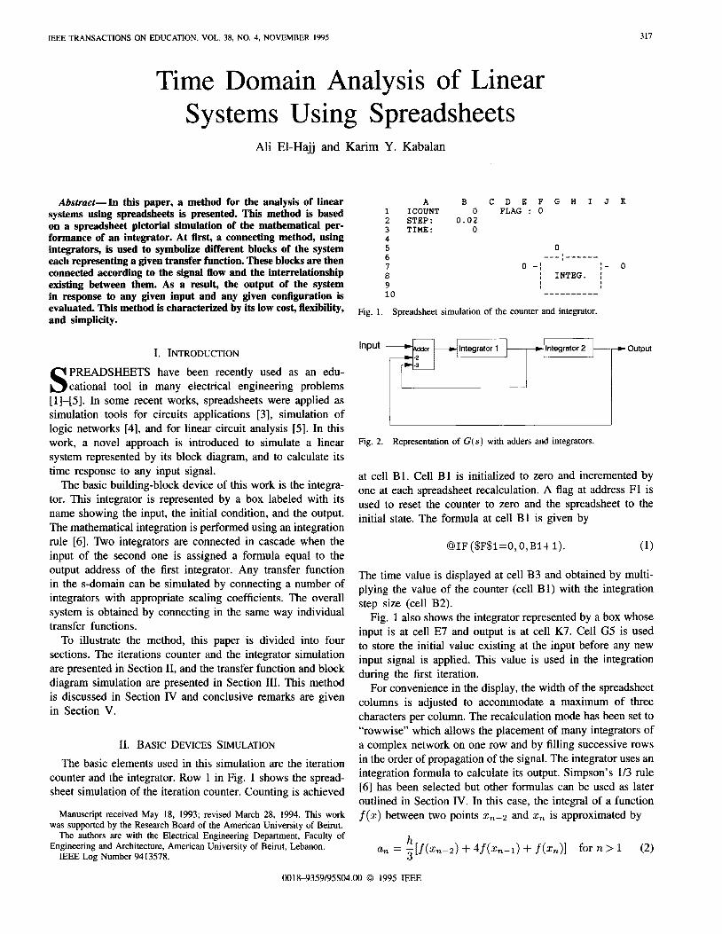
A transfer function can be simulated as a circuit with integrators and adders [7]. Since adders can be obtained by simply adding the contents of several cells, a spreadsheet simulation of a transfer function is reduced to an appropriate connection of many integrators. With a rowwise spreadsheet recalculation, these integrators must appear in the order in which the signal propagates. This is illustrated in the following example where the transfer function is given by:

(9) 1

s2 + 3 s + 2 ’ G(s) =

This transfer function is represented by the circuit of Fig. 2. Its spreadsheet representation is shown in Fig. 3. Since at any iteration the signal must traverse integrator 1 before entering integrator 2, integrator 2 must follow integrator 1 in the rowwise distribution of integrators. The outputs of these integrators are considered as inputs to integrator 1 during the

EL-HAJJ AND KABALAN: TIME DOMAIN ANALYSIS OF LINEAR SYSTEMS 319

Fig. 6. Representation of the system in Fig. 5 using adders and integrators.

Computed value

0.8

O3 -I I I 0.2 -1

* 0 0.4 0.8 1.2 1.6 2 2.4 2.8 3.2 3.6 4.0

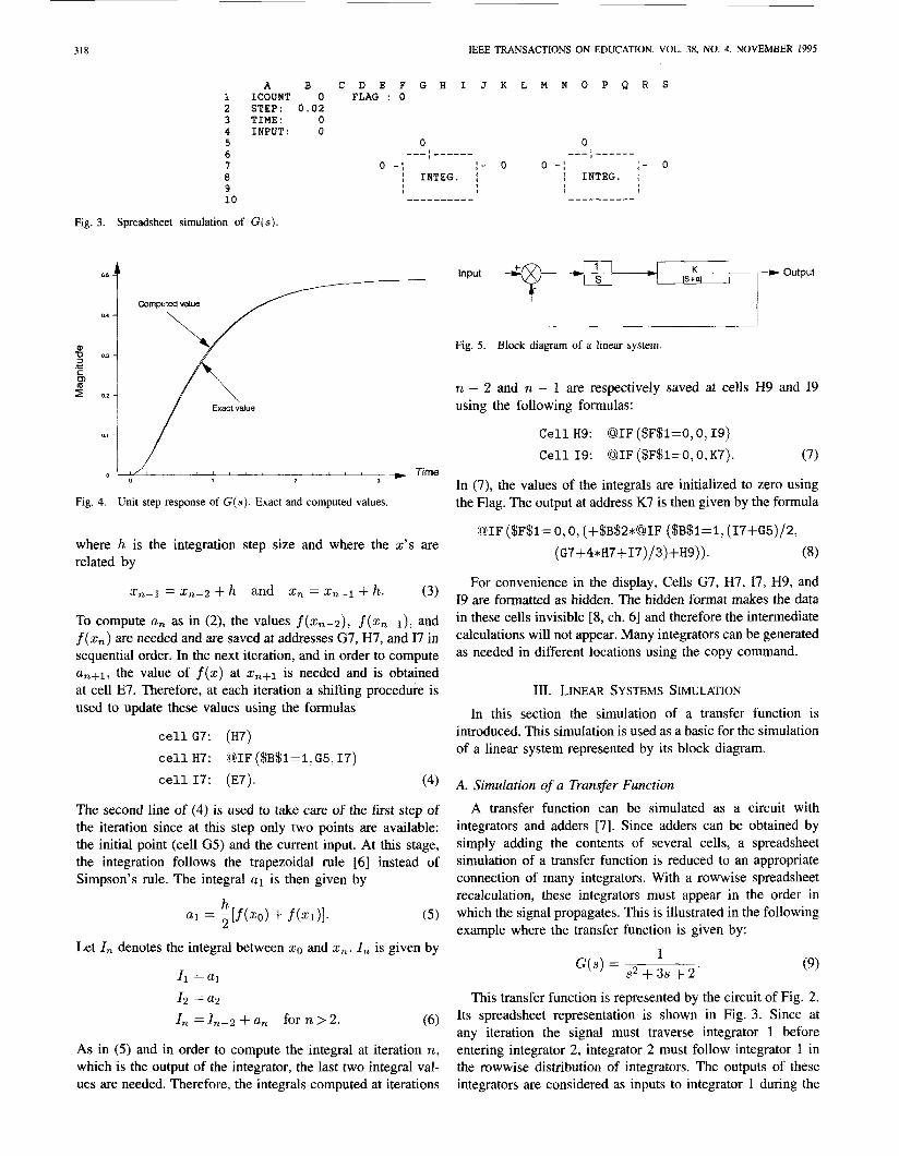
Fig. 7. Unit step response of the system in Fig. 5. Exact and computed values.

next iteration. The global input has been assigned to cell B4. Connections are accomplished by implementing the formulas

Cell E7: ($B$4-2*S7-3*K7)

Cell M7: (K7). (10)

The input can be provided as a set of values for successive iterations stored in a certain table. The input value at a certain iteration is transferred from its location in the table into the input cell (B4). For example, given 100 values to use in 100 iterations, these values can be stored in the range B8..B108 and the range A8..A108 is filled for counting purposes with the numbers 0,1, . . ,100. The following function is implemented at cell B4:

@VLOOKUP ($B$l, A8..B108,1). (1 1)

In the case where the input has an analytical expression, this expression will be implemented directly at cell B4. To store the successive output values in the range C9..C108, for example, the following formula is implemented at cell C9:

@IF ($F$l=O,O, @IF (A9=$B$l, $S$7, (29)). (12)

Equation (12) is then copied to the range ClO..C108.

The exact solution is given by For comparison, consider the unit step response of G(s).

where t is the time. Fig. 4 shows that the response given by the simulation is in good agreement with the exact solution.

Time

B. Simulation of Linear Systems

A linear system is composed of many blocks. The transfer function of each block is simulated following the procedure described above. These blocks are then connected in the same way as in connecting integrators.

For illustration, consider the control system described by the block diagram of Fig. 5. Fig. 6 shows its realization using integrators. The corresponding spreadsheet simulation in the case where a = 4 and K = 8 is the same as in Fig. 3, but were connections were established using the formulas

Cell E7: ($B$4-S7)

Cell M7: (8*K7-4*S7). (14)

Fig. 7 shows the unit step response given by the simulation which is in good agreement with the exact solution given by

IV. DISCUSSION This method has the following advantages: 1) It is low cost, because spreadsheets are already available

2) It is flexible and easy to learn, especially by spreadsheet

3) It allows easy connections between blocks. 4) Many copies of the integrator circuit can be obtained

using the spreadsheet copy command. 5 ) It allows a step-by-step study of a the evolution of a

system.

in many institutions.

users.

320 IEEE TRANSACTIONS ON EDUCATION, VOL. 38, NO. 4, NOVEMBER 1995

6) It allows the display of many variables in the system on the same graph.

7) It permits the user to study the influence of changing one or more parameters on the behavior of the system.

This method is based on connecting integrators. To simulate an integrator, an integration rule must be used. This rule can be any of the many possible implicit and explicit ones discussed in detail in many references such as in [9]. In each method, the step size must be selected to be small enough (compared to the natural time constants) to allow good accuracy, efficient computation, and stability. Error and stability analysis for different methods as function of the step size can also be found in [9].

To illustrate the presented method, Simpson’s 1/3 rule has been selected for its simplicity. This allows to achieve in many cases an acceptable accuracy, efficiency, and stability by selecting a small step size. However, when the step size is too small, a round off error becomes influencing on the solution and the computation time increases. When more efficiency is required, the integrator will be simulated following a similar approach but with a more efficient integration rule [9].

V. CONCLUSION

A general method for simulating linear systems using spreadsheets has been presented. This method is based on a spreadsheet simulation of the functions performed by several components in the system. This simulation allows the representation of systems by merely connecting the blocks of the components and the observation of the outputs in response to any input signals.

REFERENCES

[ 1 ] L. P. Huelsman, “Electrical engineering applications of microcomputer spreadsheet analysis programs,” IEEE Trans. Educ., vol. E-27, no. 2, pp. 86-92, Feb. 1984.

M. D. Rao, “Typical applications of microcomputer spreadsheets to electrical engineering problems,” ZEEE Trans. Educ., vol. E-27, no. 4, pp. 237-242, Nov. 1984. P. H. Saul, ‘‘The spreadsheet as a high level mixed mode simulation tool,” Electron. Eng., pp. S49-S55, 1991. A. El-Hajj and K. Y. Kabalan, “A spreadsheet simulation of logic networks,” IEEE Trans. Educ., vol. 34, no. 1, pp. 4346, Feb. 1991. B. J. Stanton, M. J. Drozdowski, and T. S. Duncan, “Using spreadsheets in student exercises for signal and linear system analysis,” IEEE Trans. Educ., vol. 36, no. I , pp. 62-68, Feb. 1993. S. C. Chapra and R. P. Canale, Numerical Methods for Engineers. New York McGraw-Hill, 1989. V. W. Eveleigh, Introduction to Control Systems Design. New York McGraw-Hill, 1972. C. Jorgensen, Mastering 1-2-3, 2nd ed. San Francisco: Sybex, 1986. L. 0. Chua and P. M. Lin, Computer Analysis of Electronic Cir- cuits: Algorithms and Computational Techniques. Englewood Cliffs, NJ: Prentice-Hall, 1975, chs. 11-13.

Ali El-Hajj was born in Aramta, Lebanon, in 1959. He received the B.S. degree in physics from the Lebanese University, Lebanon, in 1979, the degree on “Ingenieur” from L’Ecole Superieure d’Electricite, France, in I98 1, and the “Doctor Ingenieur” degree from the University of Rennes I, France, in 1983.

From 1983 to 1987 he was an Assistant Professor of Electrical Engineer- ing at the Lebanese University. Currently he is an Associate Professor of Electrical Engineering with the Electrical Engineering Department, Faculty of Engineering and Architecture, American University of Beirut, Lebanon. His research interests are numerical solution of electromagnetic field problems and software development.

Karim Y. Kabalan was born in Jbeil, Lebanon. He received the B.S. degree in physics from the Lebanese University, Lebanon, in 1979, and the M.S. and Ph.D. degrees in electrical engineering from Syracuse University, Syracuse, NY, in 1983 and 1985, respectively.

During the 1986 fall semester he was a Visiting Assistant Professor of Electrical Engineering at Syracuse University. Currently he is an Associate Professor of Electrical Engineering with the Electrical Engineering Depart- ment, Faculty of Engineering and Architecture, American University of Beirut, Lebanon. His research interests are numerical solution of electromagnetic field problems and software development.