/

NASA-CR-204?02 ...././.1,_ _ , ' -. /,_L_

TIME-DISTANCE HELIOSEISMOLOGY WITH TIlE MDI

INSTRUMENT: INITIAl, RESULTS _ .._3,=.2.___'--.,_

T. L. DUVALL JR.

lxdmraloO'jin Aslrom,ny and Solar t'hysic.s.

NAS/_ (;oddard ,S'lm(e l,li,_,ht ('(,ntel; Greenheh, All) 2(1771, _L S. A.

A. G. KOSOVICHEV, E H. SCHERRER, R. S. BOGART, R. I. BUSH, C. DE FOREST,

J. T. HOEKSEMA and J. SCHOU

W. W. tlan,wn E_p('rim('mal t'hv,_ic._ lx/horato/3.

Smnl_,rd Univemit3; Sta_dbr_L (bt 94305, (k S.,4.

J. l,. R. SABA, T. I). TARBELL, A. M. TITLE and C. J. WOI_FS()N

l,ockhecd Martin Ath'am'cd Te(.hnohL_y ('enter:

91-30/252, 3251 Hanover St., IJalo Allo, (7t 94304, U.S.A.

E N. MILFORD

Parallel RIII('.Y, /11(L, 41 Manzanita Ave., l,m Galo._, ('A 95030. U. S./t.

(Received 28 October, 1996- in revised form 20 November, 1996)

Abstract. In lime-dislance helioseismology, the travel lime of acoustic _r_L_'C_i_ measured betweenvarious points on the solar surface. To some approximalion, the waves can be considered to lolh)w

ray paths that depend only on a mean solar model, with the curv:.|ture of the ray paths being caused

by the increasing sound speed with depth below the surface. The travel time is allouted by various

inhomogeneities along the ray path, including flows+ temperature inhomogeneilies, and magnetic

tields. By mcasu,ing a large number of times between different locations arid tlSillg an inversion

method, it is possible lo construct 3-dimensional maps of the subsurface inhomogeneilies.

The SO[/MDI experiment on SOH() has several unique capabilities for time-distance helioseis-

mohwv The great stability of the images observed wilhoul beneli! of an inlerxenilm almosphere is

quile striking. It has made it possible l\_r us to detect the travel lime for separations of poinls assmall us 2.4 Mm in the high-resolution mode of MDI (0.6 arc sec pixel _). This has rambled the

detection of lhe supergranulation flow. Coupled with the inversion technique, we can now study the3-dimensional evolution of the flows near the solar st, rface.

1. Introduction

Three strong features of the MDi instrument on SOHO (Scherrer et al., 1995) are

the stability coming from the absence of an intervening atmosphere between the

telescope and the Sun, an orbit in continuous sunlight enabling long sequences of

'around-the-clock' observing, and the relatively high resolution compared to some

gmundbased helioseismology experiments. In this paper, we describe work that

fully exploits these features of MDI and which points to a future in which we will

be able to follow in detail the subsurface convection.

We are using a new technique coming to be known as time-distance helioseis-

mology (Duvall et al., 1993, 1996a, b; Kosovichev, 1996, Kosovichev and Duvall,

1996; D'Silva, 1996; D'Silva et al., 1996), in which the time t(:rj, :re) for acoustic

waves to travel between different surface locations (;rl,:r2) is measured from a

Solar Phv.Yics 17{I: 63 73, 1997.

(_) 1997 Khm'er Academic t'uhli,qwrv. Printed in Ih,lgium.

https://ntrs.nasa.gov/search.jsp?R=19970024842 2019-02-03T16:02:36+00:00Z

64 T. I,. I)UVAI,I, JR. I-T AI,.

cross-correlation technique. In the first approximation, the time t(:;:l, it2) depends

on inhomogeneities along a geometric ray path connecting the surface locations.

If the temperature is locally high, the waves will traverse the region more quickly

leading to a shorter travel time. If there is a flow with a component in the direction

of the ray path, the flow will tend to speed up the wave in the direction of the flow,

while slowing it down in the reciprocal direction. In this case, we are led to the

very distinctive signature of the travel time being different for waves traveling in

opposite directions between the same points. We have thought of no other effect

which can yield this signature.

A magnetic field in the region of wave travel can also lead to travel time aniso-

tropy (Duvall et al., 1996a). This is somewhat harder to isolate, as the distinctive

signature of the field is that waves travelling along the field direction have a dif-

ferent wave speed than waves travelling perpendicular to the field. For some field

geometries, it is possible to set up pairs of rays that intersect at right angles to

look for this type of signature, but it is more difficult as the two rays have different

paths except at the location where they intersect, and so other inhomogeneities can

confuse the issue. The general form of rays below the surface is shown in Figure 5.

in this paper the effect of magnetic anisotropy is not considered, because we have

studied a very quiet region.

2. Observations

For this study we have used 8.5 hours of Doppler images from January 27, 1996

taken in the high-resolution mode of MDI, which has 0.6 arcsec pixel -I . To study

convection near the surface, it is necessary to use fairly short time intervals in

order that the evolution not be too great during the observing interval. On the other

hand, it is necessary to observe for some length of time in order to get a statistical

sample of waves. The 8.5 hours is a compromise between these two competing

requirements, with the supergranule lifetime of about 1 day putting an upper limit

on how long to observe. Another point is that we need to observe for longer than

the travel time, since the correlation that we are detecting arises from the same

wave traveling from one location to the other through the subsurface layers. The

travel times used in the present study are for surface point separations in the range

6-30 Mm, and are in the range 17-34 min.

An example of a Doppler image is shown in Figure 1. There is considerable high

spatial frequency information in the image, as measurements of the point-spread

function of the instrument would predict (Scherrer et al., 1995). And in fact, with

0.6 arc sec pixel J we are somewhat oversampling the p-mode signal. With this

sampling the spatial Nyquist frequency is near spherical harmonic degree 1 = 5000.

But the fundamental mode, the lowest frequency mode in the p-mode range, crosses

the peak acoustic cutoff frequency (,-, 5.3 mHz) at degree I = 2700. Since the peak

of the power envelope is near temporal frequency 3.2 mHz, there is very little power

4OO

TIME. DISTANCF. tttI.IO,";I_ISMOI.O(;Y WITIt MI)I

High-resolution Doppler image from MDI

65

E

e"oco

"o

"Coz

I£:

o3

300

200 -

lOO

0 100 200 300 400

East-West distance, Mm

Figure/. A MDI Dopplergmm for the high-resolution lield on 27 January, 1996. While is for receding

velocity, black for approaching. The solar rotation has been removed. The image is dominated by the

iHnode oscillations and granulation. The standard de,,iation o1 the velocity values is 244 m s i

due to oscillations in the outer half (in spatial frequency) of the power spectrum.

We have used this inlk)rmation explicitly in some htter experiments in which the

images are binned 2 x 2 on board the SOHO spacecntfl to reduce the telemetry

required.

The mean power spectrum of the 8.5 hours of data is shown in Figure 2. The

spectrum is smooth, as it has been averaged over azimuth. The spatial frequency

response has been flattened to remove the effects of the point-spread function. The

excellent quality of the data is apparent. One striking thing is the large widlh of

the .f mode, which increases to _ I mHz (full-width at half maximun]) in width at

1 = 2500. It seems likely that much of this width could be caused by motions at the

surface causing the waves to be Doppler shifted. Using the standard Doppler-shifl

relation, v = Ace�l,:, we find a flow velocity, v, of 0.9 km s I fl_r a fl'equency shift,

Ace/2rc, of t:).5 mHz (one half of full-width at half maximum), and for a horizontal

wave number, /,: - /_. + 1)//? .... This is of the order of surface motions from

convection, as determined by correlation tracking or as we find later in this paper

by the time-distance technique.

66 T. L. I)UVAI.I. JR. ET AL

High-resolution power spectrum from MDI

NT

E

>:t2C

O-_D

0

0 500 1000 1500 2000 2500

angulor degree

Iqgure 2. A mean power spectrum for the g.5 hour interval studied on 27 January, 1996. The solarrotation was removed before the power spectrum was computed. The raw data was binned 2 x 2 before

lhe analysis, so the spatial Nyquist fi-equency shown is half of the maximum achievable, allhough we

get ahnost all II_e oscillation signal with the presen! analysis. The power spectrum is smooth becauseit has been avera,,ed over wave direction.

3. Analysis

To measure the travel times between different locations, we calculate the temporalcross-correlation function between the data at one location and the data within

an annulus at some great-circle distance from the point. We look at both positive

and negative lags of the correlation function, as this tells us in which direction the

waves are travelling. For example, a signal at location 1 first and later at location 2

will lead to a lag signal of one sign while a signal first at location 2 will lead to a

correlation at the opposite sign of lag.

The cross-correlation function, averaged over a number of origins, is shown in

Figure 3, along with a curve showing the time versus distance for a simple theory.

If we imagine generating a pulse of acoustic energy at the surface that propagates

along the ray paths to the distant location, we might expect to see a pulse at the

distant location. But in fact we see something that is much broader and really

looks like a wave packet with a period of 5 rain, and a width in time of about

l/bandwidth of our oscillation power spectrum, or (1 mHz) J = 17 min. This

makes sense, because the pulse that we generated at the surface had an infinite

TIMli-I)ISTAN[']i ttI{I+I[)SI/ISM()I,OGY WITI| MDI _'7

c

E

E

8o

6o

4o

20

0 50 1O0 1,50 200

distance, Mm

I.'i_,ure 3. A mean c]oss-corrclation fLnlction for the data. "lhc solid line ix a theoretical plot of the

+ Jeal-cttcjc distance. The gra'_scale pil+.'lLll+¢tilllC fOl v'.a\'cs It+ travel alon_ it rav path for the specified y " " •

is ths cro+,_,-correlatitm lunction. The first, second and third bounces +_tl¢ visible IIL'_+II+_0 If'lilt+ bO IYlil+l.

and 90 mm The line +IFLICILIIC ill each of Ih5 I'klgcs is C._.tLIsodbV the lh+lit¢ bandpass ofthe oscilkttions.

bandwidth and so could make a zero-width feature in the correlation function. As

shown earlier by Duvall el a/. (1993), the correlation function that we observe is the

Fourier translkx+m of the power spectrun] (e.g., Figure 2). The remaining fl_+aturcs

in Figure 3 correspond to the multiple bounces. If there is a correlathm observed

at time t and at distance d, tl]ere will be similar signals at 't+.× ! and tz × d, where

tz is integral, h] the ligure, the second and third bounces are seen.

For distances shorter than I0 Mm in Figure 3, we see a gap in the signal level

and then some features parallel to the abscissa, which appear quite different to tile

wave packet type of feature present ;.it larger distances. We hypothesize that the

fallolf of signal below 10 Mm distance is caused by the relative paucity of high

spatial-frequency signal in the raw signal (note that the spectrum in Figure 2 has

had the high spatial power corrected, while this has not been done to the data in

Figure 3). We also hypothesize that the large signal in the t]eighborhood of the

origin is caused by hm,,+ waveleneth+ features. To o,,et around these problems and

to separate adequately the first and second skip at short distances, we have used

cross-correhttions that have beet] filtered in phase speed (+,/,_:) with a fairly nan'ow

bandpass. An example of one of lhese cross-con+elations, covering the distance

ran,,e 4.7-8.3 Mm, is shown in Fieure 4. Our problems with lack of thne-distance

signal itt short distances and spurious signals would appear to be solved.

In some earlier work (Duvall el al., 1993), the correlation ftmction was rectified

by using the analytic signal formalism, and times were measut+ed from this signal,

68 T. I+. I)UVA1J, JR. I']T AL.

4O

3O

I0

0

0 5 10 15 20

distonce, Mm

1_7,_ure 4. Cross-correlation function after bandpass lillering in phase velocity. The signal in the target

distance range is enhanced.

-12 -8 -4 0 4 8 12 16

radial distance, Mm

Fik, ure 5. The rays going from the center Io the dillerenl annuli. The ray paths are curved because

of the increasing sound speed with depth. The sound speed increases from 7 km s i near the surface

to 35 km s _ al 1() Mm depth. The horizontal separation between surtace points is approximately

_T tithes the depth. The measured travel times are sensitive to the component of velocity altmg Ihe

particular ray palh.

which is the envelope of the correlation function. Later it was flmnd that the higher

frequency structure in the correlation function is actually a more sensitive measure

of subsurface inhomogeneities (Duvall et al.. 1996a). In that work, the location

of one of the fine-structure peaks was determined by measuring the zero crossing

of the instantaneous phase of the correlation function. For the present work+ this

has been fltrther refined (Kosovichev and Duvall, 1996). A 20-min interval in the

neighborhood of the peak in the correlation function is fit to a Gaussian wave

packet, with independent parameters for the location of the envelope, the location

of one of the fine-structure peaks, the amplitude and width of the Gaussian, and the

frequency. All the results shown are from the location of the fine-structure peak.

In Figure 5+ we show some examples of raypaths below the surface. The ray

paths are curved because of the increasing sound speed with depth in the Sun.

TIME I)ISTANCE ttI_][,IOSHSM()IX)(;Y WITtt MDI 69

A useful rule of thumb is roughly that the horizontal distance between surti_ce

rellections is 7r multiplied by the depth of the turning point of the ray. Also thelength along the ray path is four times the depth. These relations are exactly true

for a polytrope and approximately true for a real solar model.

Following Duvall et al. (1996a), we compute the mean cross-correlation fi_rwaves travelling both out from the center to the annuli and the reverse. The differ-

ence of the times measured from these cross-correlations is a measure of divergenceof the flow. It could be due to either a downflow near the central location or to

an average horizontal outflow (or inflow) near the annulus. In addition to this

divergence signal, a mean time is computed for the inward and outward waves.

To get more directional information about flows, we divide the annulus sur-

rounding a point into quadrants centered on the four directions north, south, east,

west (Duvall et al., 1996b). The signals from the four quadrants are cross-correlated

separately with the signal from the central point. The positive and negative tempor-

al lags of these four correlation functions (corresponding to the two directions of

propagation) are separated, yielding 8 correlations in all. Pairs of these correspondto each of the four cardinal directions, e.g., waves going from the eastern quad-

rant to the central point and from the central point to the western quadrant. The

average correlation function for each of the four directions is computed from these

pairs. The travel times are measured from the first skip from these correlations.Signals proportional to a flow are obtained by taking the difference of eastwardand westward times (and likewise the northward and southward times).

In Figure 6 we show the four different sets of times computed for each range ofdistance: (i) outward-inward, (ii) west-east, (iii) north-south, and (iv) mean time.

These 32 images are the input to the inversion described below.

In general, the signals for smaller annuli should be more sensitive to near-surface

inhomogeneities. The cellular pattern with the scale size of supergranulation is mostapparent in the outward-inward signal. Of course, the rays focus at the center pointsat the surface, but also reach the surface in the annuli. One interesting thing to notice

is the apparent large-scale patterns visible in the signals from the larger annuli. We

cannot distinguish directly whether these patterns are due to large scale signals nearthe surface that are being picked by the annular filter or they are due to larger scale

flows near the bottom of the ray paths visible because the rays for the larger annuli

penetrate deeper. In principle the inversion is able to distinguish between these

options, but it would be useful to have another way to see this. Maybe in futurework the signal from the second bounce could be used to make this distinction.

To check that we are seeing something with a basis in reality, we have used the

west-east and north-south signals for the smallest annulus to make an apparenthorizontal velocity to compare with the mean Doppler image over the 8.5-hour

period. The west-east and north-south times are taken as the components of a

horizontal vector and the line-of-sight component of this vector is taken. The times

are calibrated using the mean sound speed over the depth range of the rays from

a solar model. The comparison between these two is shown in Figure 7. The very

70 T.L. DUVALL JR. ET AL.

l.'i_m_, 6. Maps tfl +the limes measured end input to lhe in','ersion procedure. The 8 pictures verlic_tlly

are l_r tile 8 differen! annulus sizes. The sizes of the _mnuli are shown in the central column, sm;illesl

a! lhe top and largesl at tile bollOnl. The horizontal size o1 each image is 371) Mill. (a) Time liar

outward-gt)ing waves minus inward going waves with while displ:tyed us a negative signul. The

r.m.s, signal in the top ima,ge is 0.2 rain while in the boltom one is 0.04 rain. (b) Weslward limes

minus eastwurd times. Tile r.m.s, signal in lhe lop iln;.ige is (I.35 rain while in tile boltOlll illl;.ige is

0.19 rain. (c) Norlhward limes minus southward times. The mttgniludes are similar to b). (d) The

variation in mean time for tile average ol +inward and t_utward times ,aith ;.i neg:ttive signal displayed

as white. The r.m.s, of the top image is 0.05 rain while for lhe bottom image it is 0.08 rain. A

correlation of this signal with the loc;ttion of tile magnetic features can be seen, in agreement w, iltl

results of Duv_lll _'t a/. ( 1996a, h). (e) The magnetic field in Ihis region, as observed with tile MDI

instrument. (f)The mean Doppler sign_tl observed Ior lhe 8.5 hour interval. ]'his shows mainly lhe

horizontal motions ol +superg,anules. Near lhe center of tile disk <lower center t_l picture) Ihe signal

lrom horizolital flows disappears I-,ecause it is perpendicuktr to the line of sight. The images in a

single column ;ire all on the same scale.

TIME [)ISTANCI:_ tlI_I.I()SIilSMOI.O(iY \',,'ITtt MI)I 7 I

I"ik, mu 7. A comparison between a silnulaled Doppler image using lhe images lronl tile top line of

Figures 6(b} and 6(c) and the mean Doppler image for the 8.5 hotll_; (Figure 6(f)}. (a) The simulated

image. The east west and Ilorth-soulh times are combined and then projected onto the line of sighl.

(b) The mcan Doppler image for the g.5 hours.

400 .::; _:_: :7"7_';',.'":::'Lr.','.:-: "._:; :::::::::::::::::::::: ::._; _£':_J",:_.?,_" ::":{:', ='-_:,?:" :a',_: "-'_::: ":'_:'_J IYL_!: _'_!::ri::.*2"__

200 ,-'-1_.:: !!_,..:: t,?'..:.!!: . t; " ::'i' _;;": _' ::. /_:":, _'' :: "_': ,::-..'r

_;':! ,. :': i<' " :. _ '.':"_ { : :;:_'c:-...: _ ,,,, " :::q:;_ "_::_: :.' '-_::::::_-_'_'i

_i!: :!:: .::i( ;':.!- ill/,. : ; _;-:_:_ rTi "_" ! _-: <-_: '4.,'::::i : :t{a{-; i-:.

0 I O0 200 300 400

Eost-Wesl. dislonce, Mm

Figure & A comparison between the absolulc value of magnetic field (in color) and Ihe sinmlated

surface velocity from the time distance pictures (arrows). The longest arrow is for 1 km s _ velocity.

high correlation is apparent. The correlation coefficient between these two imagesis 0.74. The signals disappear near the disk center because the supergranulation

velocity is predominantly horizontal which is perpendicular to our line of sight atdisk center.

Another check on our understanding is shown in Figure 8. The same components

of east-west and north-south velocity used in Figure 7 are combined to show

horizontal velocity vectors. The vectors are overlaid on an image of the absolute

value of magnetic feld. We see that the magnetic field tends to lie at the boundaries

72

E

o

",5

"C'ozI

.z:

300

1 O0

..... =' _,2_".".0 !t:_!:_'_! ........ !_; '-!

0 1 O0 200 300 400

East-West dlstonce, Mrn _

Figure 9. The horizontal flows near the surface from the inversion procedure are shown as vectors.

The vectors are over]aid on the inverted temperature structure shown in blue and red for hotter and

cooler.

of the cellular outflows, in agreement with our general picture of the magneticnetwork.

The time- distance maps are used in a ray-theory inversion (Kosovichev, 1996;

Kosovichev and Duvall, 1996). The region of the Sun is separated into a 3-D grid

of inhomogeneities with the same horizontal sampling interval as the input images

(4.3 Mm) and an equal increment in depth covering the same depth range as the

input data. The number of grid points in depth is taken to be the same as the

number of input images (in this case, 8). Each 3-D grid point has lbur independent

variables, the three components of flow velocity and a sound speed inhomogeneity.

No attempt is made to satisfy any conservation equations, such as the continuity

equation.

In Figure 9, we show the inversion results for the surface layer. The high

correlation with the mean Doppler image is apparent. One advantage of studying

near-surface regions is that we do have extra information for comparison at the

surface that we would not have for the deep interior.

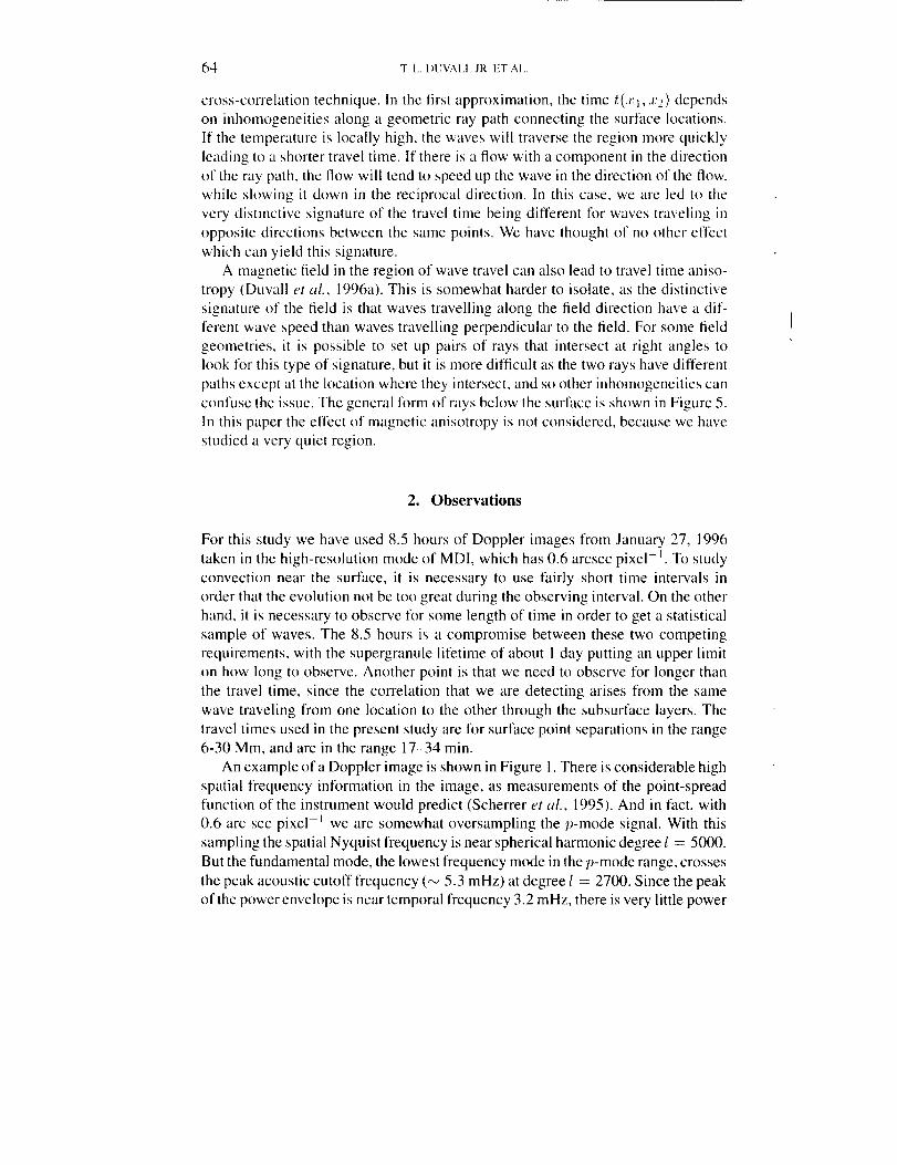
In Figure 10 we present a vertical cut showing the subsurface flows and sound

speed inhomogeneities. It would appear that the pattern of horizontal motions at

the surface only persists to a few Megameters in depth. But it is probably still

premature to draw strong conclusions because of the newness of the method.

TIMt- I)ISTANCI.: ttEI,I()SF, ISMOIA)GY WITH Ml)l 73

/"i,k,,rc I{L A velliC_.d cut showing the Co111po11CIll o1 llow in the plane. The llow is again shown as

vcclo]-s and is overlaid on the tu'll/pcr;.tlure inhomogen¢ifies.

4. Conclusions

We have shown that there is detailed information about the subsurface inhomo-

geneities contained in the helioseismology data. We have also shown it should be

possible to extract this information and have shown some tirst-order attempts to do

so. We w,ould appear to have an exciting new window into the solar interior.

Acknowledgements

The authors acknowledge many years of effort by the engineering and support staff

of the MDI development team at the Lockheed Palo Alto Research Laboratory (now

Lockheed-Martin Advanced Technology Center) and the SOl development team

al Stanford Universily. SOHO is a project of international cooperation between

ESA and NASA. This research is supported by the SOI-MDI NASA contract

NAGS-3077 at Stanford University.

References

D'Silva. S.: 1996, Asm*phv,v .I. 469, 964.D'Silva, S., Duvall, T. L, Jr., ,leffcries, S. M., and H;.lrvcy, J. W.: 1006. A,_.DT_I)IIV,'_. ,1. 471, 1030.

l)uvall, T. l,., Jr., Jefferies, S. M., H:.ll"Vey, J. W., and Pomerantz. M. A.: 1993. NalHrc 362, 430.

I)u_all. T. I,., ,h., l)'Silva, S., Jefferies, S. M., Harvey, J. W.. and Schou, J.: 19t)6a, Nal,rc 379, 235.

Du vail, T. [,., J ]., Kt_so', ichev, A. G., SchcrreF, P. H.. _.lnd M il ford, P. N.: 199_"_b, Ihdl. Am. A,stn m. ,S'o_.

188, S9g.

Kosovichev, A. G.: 1996. Aslro/dlv,s. ,/. 461, 1,55.

Kosovichev, A. (;. and Duvall, T. [,., Jr.: 1996, ill J. Chrislensen-|)alsgaard and I:. Pijpers (eds.), 'Solar

Convection and Oscill:.llions :.llld their Relationship', Proc. of S('()'Rd '_)& Worl, dmp, Aarhus,

Denmark, May 27 31, 1996, Kluwer Academic Publishers, Dordrcchl, Holland, in press.

Scherrer, P. H., Bogalt, R. S., Bu,,h, R. I.• ttoeksema, J. T., Kosovichev, A. G., Schou, J., Rosenberg, W.,

Springer, L., Tarbell, T. I)., Title, A., Wollson, C. J., Zayer, I., and the MDI Engineering Team:

1995, Solm" Phys. 162, 129.