TIME-DISTANCE HELIOSEISMOLOGY: THE FORWARD PROBLEM

TIME-DISTANCE HELIOSEISMOLOGY: THE FORWARD PROBLEM FOR RANDOMDISTRIBUTED SOURCES

L. Gizon and A. C. Birch

W.W.Hansen Experimental Physics Laboratory, StanfordUniversity, Stanford, CA 94305Received 2001 April 24; accepted 2002 February 4

ABSTRACT

The forward problem of time-distance helioseismology is computing travel-time perturbations that resultfrom perturbations to a solar model. We present a new and physically motivated general framework for cal-culations of the sensitivity of travel times to small local perturbations to solar properties, taking into accountthe fact that the sources of solar oscillations are spatially distributed. In addition to perturbations in soundspeed and flows, this theory can also be applied to perturbations in the wave excitation and damping mecha-nisms. Our starting point is a description of the wave field excited by distributed random sources in the upperconvection zone. We employ the first Born approximation to model scattering from local inhomogeneities.We use a clear and practical definition of travel-time perturbation, which allows a connection between obser-vations and theory. In this framework, travel-time sensitivity kernels depend explicitly on the details of themeasurement procedure. After developing the general theory, we consider the example of the sensitivity ofsurface gravity wave travel times to local perturbations in the wave excitation and damping rates. We deriveexplicit expressions for the two corresponding sensitivity kernels. We show that the simple single-source pic-ture, employed in most time-distance analyses, does not reproduce all of the features seen in the distributed-source kernels developed in this paper.

Subject headings: scattering — Sun: helioseismology — Sun: interior — Sun: oscillations — waves

1. INTRODUCTION

Time-distance helioseismology, introduced by Duvall etal. (1993b), has yielded numerous exciting insights into theinterior of the Sun. This technique, which gives informationabout travel times for wave packets moving between anytwo points on the solar surface, is an important complementto global-mode helioseismology, as it is able to probe sub-surface structure and dynamics in three dimensions. Someof the main results concern flows and wave-speed perturba-tions underneath sunspots (Duvall et al. 1996; Kosovichev,Duvall, & Scherrer 2000; Zhao, Kosovichev, & Duvall2001), large-scale subsurface poleward flows (Giles et al.1997), and supergranulation flows (Duvall &Gizon 2000).

The interpretation of time-distance data can be dividedinto a forward and an inverse problem. The forward prob-lem is to determine the relationship between the observatio-nal data (travel times ��) and internal properties (q�).Generally, this relationship is sought in the form of a linearintegral equation,

�� ¼X�

Z�dr �q�ðrÞK�ðrÞ ; ð1Þ

where the �q�ðrÞ represent the deviations in internal solarproperties from a theoretical reference model. The index �refers to all relevant types of independent perturbations,such as sound speed, flows, or magnetic field. The integralR� dr denotes spatial integration over the volume of theSun. The kernels of the integrals, K�ðrÞ, give the sensitivityof travel times to the perturbations to the solar model. Theinverse problem is to invert the above equation, i.e., to esti-mate �q�, as a function of position r, from the observed �� .In this paper we consider only the forward problem.

An accurate solution to the forward problem is necessaryfor making quantitative inferences about the Sun fromtime-distance data. There have been a number of previous

efforts to understand the effect of local perturbations ontravel times. D’Silva et al. (1996), Kosovichev (1996), andZhao et al. (2001) used geometrical acoustics to describe theinteraction of acoustic waves with sound-speed perturba-tions and flows. Bogdan (1997) argued that a finite-wave-length theory is needed. Birch & Kosovichev (2000) solvedthe linear forward problem for sound-speed perturbations,in the single-source approximation. Jensen, Jacobsen, &Christensen-Dalsgaard (2000) solved a weakly nonlinearforward problem for sound-speed perturbations, in the sin-gle-source approximation, and proposed the use of Fresnel-zone–based travel-time kernels. Bogdan, Braun, & Lites(1998) used a normal mode approach to compute travel-time perturbations in a model sunspot. Woodard (1997)estimated the effect of wave absorption by sunspots ontravel times. This important work, which required a modelfor random distributed wave sources, is one of the primarymotivations for obtaining a general theory for travel-timesensitivity kernels. The model developed by Woodard(1997) employs, however, the approximation that wavedamping affects only the amplitude of transmitted waves,ignoring scattering. Birch et al. (2001) tested the accuracy oftravel times obtained in the Born approximation, whichmodels single scattering from local inhomogeneities.Although the above-mentioned efforts represent substantialprogress, there is not yet a general procedure for relatingactual travel-time measurements to perturbations to a solarmodel that takes into account random distributed sourcesfor solar oscillations, despite a preliminary study by Gizon& Birch (2001).

The first part of this paper (x 2) is an attempt to synthesizeand extend the current knowledge into a flexible frameworkfor the computation of the linear sensitivity of travel timesto local inhomogeneities. We start from a physical descrip-tion of the wave field, including wave excitation and damp-ing. We incorporate the details of the measurement

The Astrophysical Journal, 571:966–986, 2002 June 1

# 2002. The American Astronomical Society. All rights reserved. Printed in U.S.A.

966

procedure. Two other key ingredients of our approach arethe single-scattering Born approximation and a clear obser-vational definition of travel time, both taken from the geo-physics literature (e.g., Tong et al. 1998; Zhao & Jordan1998; Marquering, Dahlen, & Nolet 1999). The main differ-ence between the geophysics and helioseismology problemsis that helioseismology deals with multiple random wavesources as opposed to a single isolated source.

The second part of this paper (x 3) is an example calcula-tion of travel time kernels for surface gravity waves. Thepurpose is to demonstrate the application of the generaltheory described in x 2. We compute travel-time kernels forlocal perturbations in source strength and damping rate. Inour model, these perturbations are confined to the surfaceand therefore are computationally convenient, as we obtaintwo-dimensional kernels. Localized source and dampingperturbations are interesting and not yet well understood.For this example, we also compare these kernels with ker-nels calculated in the single-source picture (Birch & Kosovi-chev 2000; Jensen et al. 2000), in which distributed randomsources are replaced by an artificial causal source placed atone of the observation points. We show that the single-source kernels do not reproduce all the features seen in thedistributed-source kernels.

2. GENERAL THEORY

2.1. Definition of Travel Times

The fundamental data of modern helioseismology arehigh-resolution Doppler images of the Sun’s surface. In gen-eral, the filtered line-of-sight projection of the velocity field

can be written as

� ¼ F ll x vn o

; ð2Þ

where v is the Eulerian velocity and ll is a unit vector in thedirection of the line of sight. The operator F describesthe filter used in the data analysis, which includes the timewindow (time duration T), instrumental effects, and otherfiltering.

The basic computation in time-distance helioseismologyis the temporal cross-correlation, C(1, 2, t), between the sig-nal, �, measured at two points, 1 and 2, on the solar surface,

Cð1; 2; tÞ ¼ 1

T

Z 1

�1dt0 �ð1; t0Þ�ð2; t0 þ tÞ ; ð3Þ

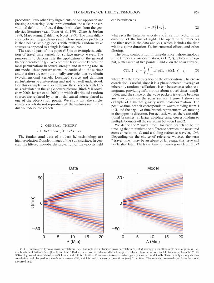
where T is the time duration of the observation. The cross-correlation is useful, since it is a phase-coherent average ofinherently random oscillations. It can be seen as a solar seis-mogram, providing information about travel times, ampli-tudes, and the shape of the wave packets traveling betweenany two points on the solar surface. Figure 1 shows anexample of a surface gravity wave cross-correlation. Thepositive-time branch corresponds to waves moving from 1to 2, and the negative-time branch represents waves movingin the opposite direction. For acoustic waves there are addi-tional branches, at larger absolute time, corresponding tomultiple bounces off the surface in between 1 and 2.

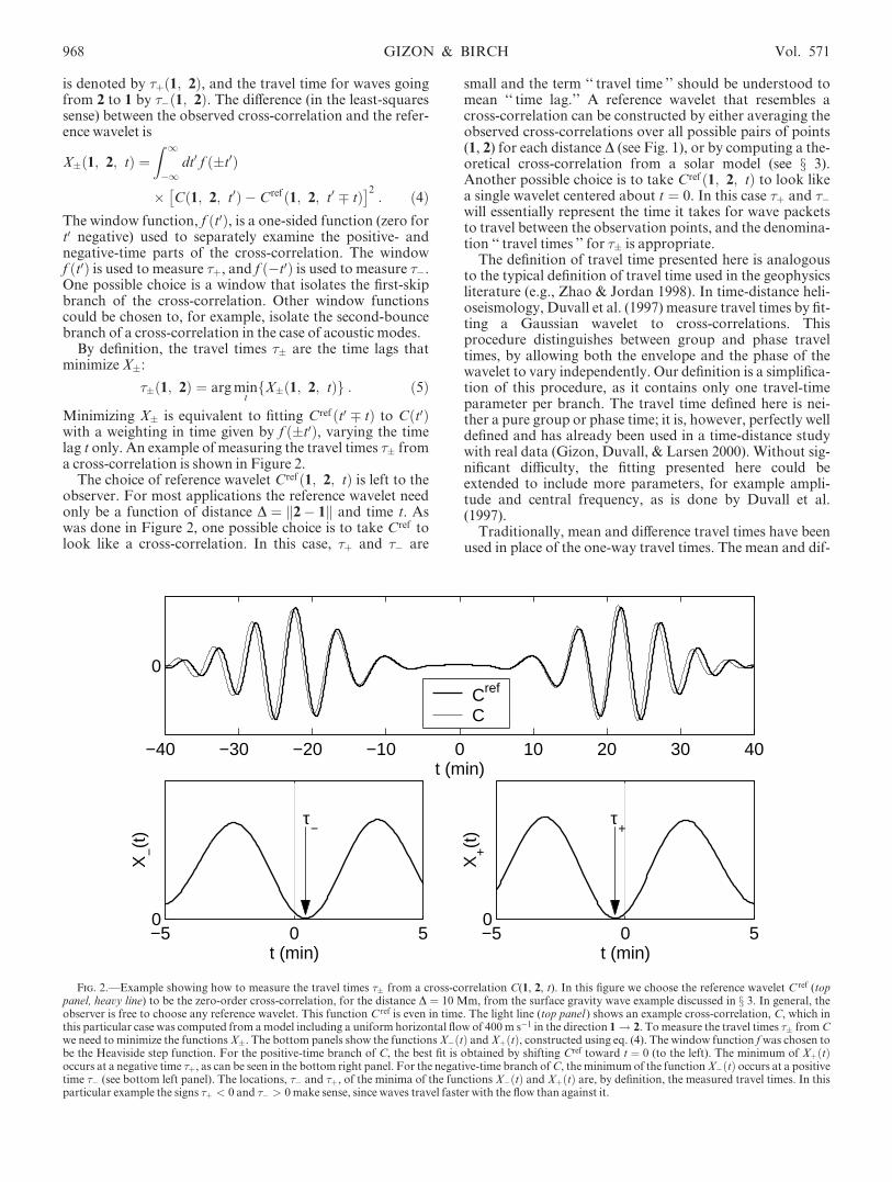
We define the ‘‘ travel time ’’ for each branch to be thetime lag that minimizes the difference between the measuredcross-correlation, C, and a sliding reference wavelet, Cref .Depending on the choice of reference wavelet, the term‘‘ travel time ’’ may be an abuse of language; this issue willbe clarified later. The travel time for waves going from 1 to 2

Fig. 1.—Surface gravity wave cross-correlations. Left: Example of an observed cross-correlation C(1, 2, t) averaged over all possible pairs of points (1, 2),as a function of distance D ¼ 2� 1k k and time t. Red refers to positive values and blue to negative values. The observations are 8 hr time series from theMDI/SOHO high-resolution field of view (Scherrer et al. 1995). The filterF is chosen to isolate surface gravity waves around 3 mHz. This spatially averaged cross-correlation could be used as the reference wavelet Cref , which is used to measure travel times (see x 2.1). Right: Theoretical cross-correlation from the modeldiscussed in x 3.

TIME-DISTANCE HELIOSEISMOLOGY 967

is denoted by �þð1; 2Þ, and the travel time for waves goingfrom 2 to 1 by ��ð1; 2Þ. The difference (in the least-squaressense) between the observed cross-correlation and the refer-ence wavelet is

X�ð1; 2; tÞ ¼Z 1

�1dt0 f ð�t0Þ

� Cð1; 2; t0Þ � Crefð1; 2; t0 � tÞ� �2

: ð4ÞThe window function, f ðt0Þ, is a one-sided function (zero fort0 negative) used to separately examine the positive- andnegative-time parts of the cross-correlation. The windowf ðt0Þ is used to measure �þ, and f ð�t0Þ is used to measure ��.One possible choice is a window that isolates the first-skipbranch of the cross-correlation. Other window functionscould be chosen to, for example, isolate the second-bouncebranch of a cross-correlation in the case of acoustic modes.

By definition, the travel times �� are the time lags thatminimizeX�:

��ð1; 2Þ ¼ argmintfX�ð1; 2; tÞg : ð5Þ

Minimizing X� is equivalent to fitting Crefðt0 � tÞ to Cðt0Þwith a weighting in time given by f ð�t0Þ, varying the timelag t only. An example of measuring the travel times �� froma cross-correlation is shown in Figure 2.

The choice of reference wavelet Crefð1; 2; tÞ is left to theobserver. For most applications the reference wavelet needonly be a function of distance D ¼ 2� 1k k and time t. Aswas done in Figure 2, one possible choice is to take Cref tolook like a cross-correlation. In this case, �þ and �� are

small and the term ‘‘ travel time ’’ should be understood tomean ‘‘ time lag.’’ A reference wavelet that resembles across-correlation can be constructed by either averaging theobserved cross-correlations over all possible pairs of points(1, 2) for each distance D (see Fig. 1), or by computing a the-oretical cross-correlation from a solar model (see x 3).Another possible choice is to take Crefð1; 2; tÞ to look likea single wavelet centered about t ¼ 0. In this case �þ and ��will essentially represent the time it takes for wave packetsto travel between the observation points, and the denomina-tion ‘‘ travel times ’’ for �� is appropriate.

The definition of travel time presented here is analogousto the typical definition of travel time used in the geophysicsliterature (e.g., Zhao & Jordan 1998). In time-distance heli-oseismology, Duvall et al. (1997) measure travel times by fit-ting a Gaussian wavelet to cross-correlations. Thisprocedure distinguishes between group and phase traveltimes, by allowing both the envelope and the phase of thewavelet to vary independently. Our definition is a simplifica-tion of this procedure, as it contains only one travel-timeparameter per branch. The travel time defined here is nei-ther a pure group or phase time; it is, however, perfectly welldefined and has already been used in a time-distance studywith real data (Gizon, Duvall, & Larsen 2000). Without sig-nificant difficulty, the fitting presented here could beextended to include more parameters, for example ampli-tude and central frequency, as is done by Duvall et al.(1997).

Traditionally, mean and difference travel times have beenused in place of the one-way travel times. The mean and dif-

−40 −30 −20 −10 0 10 20 30 40

0

t (min)

Cref

C

−5 0 50

X−(t

)

t (min)

τ−

−5 0 50

X+(t

)

t (min)

τ+

Fig. 2.—Example showing how to measure the travel times �� from a cross-correlation C(1, 2, t). In this figure we choose the reference wavelet C ref (toppanel, heavy line) to be the zero-order cross-correlation, for the distance D ¼ 10 Mm, from the surface gravity wave example discussed in x 3. In general, theobserver is free to choose any reference wavelet. This function C ref is even in time. The light line (top panel ) shows an example cross-correlation, C, which inthis particular case was computed from amodel including a uniform horizontal flow of 400m s�1 in the direction 1 ! 2. Tomeasure the travel times �� fromCwe need to minimize the functionsX�. The bottom panels show the functionsX�ðtÞ andXþðtÞ, constructed using eq. (4). The window function fwas chosen tobe the Heaviside step function. For the positive-time branch of C, the best fit is obtained by shifting Cref toward t ¼ 0 (to the left). The minimum of XþðtÞoccurs at a negative time �þ, as can be seen in the bottom right panel. For the negative-time branch ofC, theminimumof the functionX�ðtÞ occurs at a positivetime �� (see bottom left panel). The locations, �� and �þ, of the minima of the functions X�ðtÞ and XþðtÞ are, by definition, the measured travel times. In thisparticular example the signs �þ < 0 and �� > 0make sense, since waves travel faster with the flow than against it.

968 GIZON & BIRCH Vol. 571

ference travel times are obtained from the one-way traveltimes by

�mean ¼ 12 ð�þ þ ��Þ ; ð6Þ

�diff ¼ �þ � �� : ð7ÞThe motivation behind using �mean and �diff is that sound-speed perturbations are expected to contribute mostly to themean travel time and flows to the travel-time difference(e.g., Kosovichev &Duvall 1998).

The definition of travel-time perturbations described hereleaves observers free to measure without reference to a solarmodel. We note, however, that in order for a proper inter-pretation of measured travel-time perturbations to be madeit is essential for observers to report their choices of refer-ence wavelet Cref , window function f, and filter F. A solarmodel is only necessary for the next step, the interpretationof travel-time perturbations in terms of local perturbationsto a solar model, to which we now turn.

2.2. Interpretation of Travel Times

The goal of time-distance helioseismology is to estimatethe internal solar properties that produce model travel timesthat best match observed travel times. To achieve this, weneed to know how to compute the travel times for a particu-lar solar model. In order to make the inverse problem feasi-ble, we also need to linearize the forward problem around abackground state that is close to the Sun.

A background solar model is fully specified by a set ofinternal properties (density, pressure, etc.), which we denoteby q�ðrÞ for short. Standard solar models provide a reason-able background state. In the background state the cross-correlation and the travel times are C0 and �0�, respectively.We then consider small perturbations, �q�ðrÞ, to the solarproperties. These perturbations could include, for example,local changes in density, sound speed, or flows. The differ-ence between the resulting cross-correlation, C, and thebackground cross-correlation we denote by �C,

�Cð1; 2; tÞ ¼ Cð1; 2; tÞ � C0ð1; 2; tÞ : ð8ÞLikewise, the perturbed travel times �� are

��ð1; 2Þ ¼ ��ð1; 2Þ � �0�ð1; 2Þ : ð9ÞThe travel times ��ð1; 2Þ are measured from the cross-cor-relation Cð1; 2; tÞ. The reference times �0� are the traveltimes that would be measured if the Sun and the back-groundmodel were identical.

Since we are considering small changes in the solar model,the correction to the model cross-correlation, �C, will alsobe small. As a result, we can linearize the dependence of thetravel-time perturbations �� on �C. The algebra is detailedin Appendix A. The result of this calculation can be writtenas

��ð1; 2Þ ¼Z 1

�1dtW�ð1; 2; tÞ�Cð1; 2; tÞ : ð10Þ

The functions W� depend on the zero-order cross-correla-tionC0, the reference waveletCref , and the window functionf, and are given in equation (A7). The sensitivity of �� to�C is given by the weight functionsW�. We emphasize thatthe travel-time perturbations �� are proportional to �C,which is a first-order perturbation to the background solarmodel. We interpret the right-hand side of equation (10) asa model for the difference between the observed travel times

and the theoretical travel times in the background solarmodel.

The source of solar oscillations is turbulent convectionnear the solar surface (e.g., Stein 1967). As a result, the sig-nal � and the cross-correlation C are realizations of a ran-dom process. In general, a random variable is fullycharacterized by its expectation value and all of its higherorder moments. As a result, to describe a travel-time pertur-bation �� we need its expectation value (ensemble average)as well as its variance, etc. In this paper we consider only theexpectation value. A calculation of the variance of the traveltimes would be essential to characterize the realization noisein travel time measurements. An accurate estimate of thenoise in travel time measurements is important for solvingthe inverse problem.

In this paper we only compute the expectation values oftravel-time perturbations and cross-correlations. This rep-resents a first and necessary step. Note in addition thatunder the assumptions of the Ergodic theorem (e.g.,Yaglom 1962) the cross-correlations (hence travel times)tend to their expectation values as the observational timeinterval increases.

2.3. Modeling the Observed Signal

In order to obtain the cross-correlation, C0, and its first-order perturbation, �C, we need to compute the observable,�, defined in equation (2), and therefore the wave velocity v.Linear oscillations are governed by an equation of the form(e.g., Gough 1993)

Lv ¼ S : ð11ÞThe vector S denotes the source of excitation for the waves.The linear operator L, acting on v, should encompass allthe physics of wave propagation in an inhomogeneousstratified medium permeated by flows and magnetic fields.Damping processes should also be accounted for in L. Anexplicit expression for the operator L including steadyflows is provided by Lynden-Bell & Ostriker (1967). Bogdan(2000) includes magnetic field.

We now expand L, v, and S into zero- and first-ordercontributions, which refer to the background solar modeland to the lowest order perturbation to that model:

L ¼L0 þ �L ; ð12Þv ¼ v0 þ �v ; ð13ÞS ¼ S0 þ �S : ð14Þ

The operator �L depends on first-order quantities such aslocal perturbations in density, sound speed, and dampingrate, as well as flows and magnetic field. In general, one cancontemplate time-dependent perturbations. There are, how-ever, many interesting structures on the Sun (e.g., supergra-nules, meridional flow, moat flows) that are approximatelytime independent on the timescale on which time-distancemeasurements are made (at least several hours). As a result,for the sake of simplicity, we only consider time-independ-ent perturbations. These perturbations, which we denote by�q�ðrÞ for short, are thus only functions of position r in thesolar interior.

To lowest order, equation (11) reduces to

L0v0 ¼ S0 : ð15Þ

In order to solve this equation, we introduce a set of causal

No. 2, 2002 TIME-DISTANCE HELIOSEISMOLOGY 969

Green’s vectorsG i defined by

L0G iðx; t; s; tsÞ ¼ eeiðsÞ�Dðx� sÞ�Dðt� tsÞ ; ð16Þ

where the eeiðsÞ are three orthogonal basis vectors at thepoint s, and �D is the Dirac delta function. The vectorG iðx; t; s; tsÞ is the velocity at location x and time t thatresults from a unit impulsive source in the eei direction attime ts and location s. Note that the vector G i does not ingeneral point in the direction of eei. Guided by equation (2),we define the zero-order Green’s functions for the observ-able �:

Giðx; t; s; tsÞ ¼ F llðxÞ xG iðx; t; s; tsÞn o

: ð17Þ

In terms ofGi, the unperturbed signal reads

�0ðx; tÞ ¼Z�ds

Z 1

�1dts G

iðx; t; s; tsÞS0i ðs; tsÞ : ð18Þ

The sum is taken over the repeated index i, as is done for allrepeated indexes throughout this paper.

To the next order of approximation, equation (11) gives

L0 �v ¼ ��L v0 þ �S : ð19Þ

This is the single-scattering Born approximation (e.g.,Sakurai 1995). The first-order Born approximation has beenshown to work for small perturbations (e.g., Hung, Dahlen,& Nolet 2000; Birch et al. 2001). We note that equation (19)is of the same form as equation (15): the term ��L v0 þ �Sappears as a source for the scattered wave velocity �v. Thesolution to equation (19) is thus

�vðx; tÞ ¼Z�ds

Z 1

�1dts G

iðx; t; s; tsÞ

� ��Lv0ðs; tsÞ þ �Sðs; tsÞ� �

i; ð20Þ

where f. . .gi denotes the ith component of the vector insidethe curly braces.

By expressing the zero-order velocity v0 in terms of theGreen’s function and the source, and using equation (20)and �� ¼ Ffll x �vg, the perturbed signal can be written as

��ðx; tÞ ¼� Z

�dr

Z 1

�1dt0

Z�ds

Z 1

�1dts G

iðx; t; r; t0Þ

� ��LG jðr; t0; s; tsÞ� �

iS0j ðs; tsÞ

�

þZ�ds

Z 1

�1dts G

iðx; t; s; tsÞ�Siðs; tsÞ : ð21Þ

We recall that the operator �L contains the first-order per-turbations to the solar model, �q�ðrÞ. The first term in theabove equation contains two Green’s functions; it repre-sents the contribution to ��ðx; tÞ that comes from a wavethat is created by the source at location s at time ts, is scat-tered at time t0 by the perturbations at location r, and thenpropagates to the location x. The details of the scatteringprocess are encoded in the operator �L. The second termresults from the perturbation to the source function, andinvolves only a single Green’s function, which propagateswaves from the location and time of the source to the obser-vation location and time. As we now have �0 and ��, we cannext compute the zero- and first-order cross-correlations,C0 and �C.

2.4. Temporal Cross-Correlation

We remind the reader that we only want to compute theexpectation value of the cross-correlation (see x 2.2). In therest of this paper, cross-correlations stand for their expecta-tion values. From equation (3) and the equation for �0

derived in the previous section (eq. [18]), we deduce a gen-eral expression for the zero-order cross-correlation:

C0ð1; 2; tÞ ¼ 1

T

Zdt0 ds dts ds

0 dt0s M0ijðs; ts; s0; t0sÞ

� Gi 1; t0; s; tsð ÞGjð2; t0 þ t; s0; t0sÞ ; ð22Þ

with

M0ijðs; ts; s0; t0sÞ ¼ E S0

i ðs; tsÞS0j ðs0; t0sÞ

� �; ð23Þ

where E½. . .� denotes the expectation value of the expressionin square brackets. For the sake of readability, we haveomitted the limits of integration in equation (23). Thematrix M0 gives the correlation between any two compo-nents of S0, measured at two possibly different positions.

No assumption has been made aboutM0 to obtain equa-tion (22). With the assumptions of stationarity in time andhomogeneity and isotropy in the horizontal direction, M0

only depends on the time difference ts � t0s, the horizontaldistance between s and s0, and their depths. Further assump-tions could be made in order to simplify the computation ofequation (22). In the spirit of Woodard (1997), one mightassume that the sources are spatially uncorrelated or arelocated only at a particular depth. A better approach mightbe to obtain the statistical properties of S0 from recentnumerical simulations of solar convection (e.g., Stein &Nordlund 2000) or observations of photospheric convection(e.g., Title et al. 1989; Chou et al. 1991; Strous, Goode, &Rimmele 2000). Furthermore, a comparison of models andobservations of the power spectrum of solar oscillations canbe used to constrain the depths and types of sources (e.g.,Duvall et al. 1993a).

We now perturb equation (3) and take the expectationvalue to obtain

�Cð1; 2; tÞ ¼ 1

T

Z 1

�1dt0 E

h��ð1; t0Þ�0ð2; t0 þ tÞ

þ �0ð1; t0Þ ��ð2; t0 þ tÞi: ð24Þ

The function �C has two contributions, one from the per-turbation to the wave operator, �CL, and one from thesource perturbation, �CS:

�C ¼ �CL þ �CS : ð25Þ

Using the expressions for �0 and �� given by equations(18) and (21), we obtain the perturbation to the cross-corre-lation resulting from a change in the wave operatorL:

�CLð1; 2; tÞ ¼ 1

T

Z�dr

Zdt0 dt00 ds dts ds

0 dt0s

� ��LG iðr; t00; s; tsÞ� �

kM0

ijðs; ts; s0; t0sÞ

�hGjð2; t0 þ t; s0; t0sÞGkð1; t0; r; t00Þ

þ Gjð1; t0; s0; t0sÞGkð2; t0 þ t; r; t00Þi: ð26Þ

The above equation, which gives the perturbation to thecross-correlation due to scattering, has two components,


illustrated in Figure 3a. The first component comes from thecorrelation of the scattered wave at 1 with the direct wave at2, i.e., ��ð1; t0Þ�0ð2; t0 þ tÞ, and the second componentcomes from �0ð1; t0Þ��ð2; t0 þ tÞ. Both of these componentsappear in equation (26) as the product of three Green’sfunctions. From the term ��ð1; t0Þ�0ð2; t0 þ tÞ there is oneGreen’s function for the wave that goes directly from s0 to 2,which gives �0(2). There is a second Green’s function for thewave that is created at s and travels to r, and the thirdGreen’s function takes the scattered wave from r to 1, whichgives ��(1). The term �0ð1; t0Þ��ð2; t0 þ tÞ can be understoodby switching the roles of 1 and 2. The scattering process isdescribed by the operator �L, which depends on the pertur-bations �q�ðrÞ. The Green’s function G is used for wavesthat arrive at an observation point as it gives the response of� to a source. The Green’s vectors G i are used to propagatethe wave velocity from a source to the scattering point, asthe scattered wave depends on the vector velocity of theincoming wave.

The cross-correlation is also sensitive to changes in thesource function. The first-order perturbation resulting froma small change in the source function can be written as (from

eqs. [18] and [21])

�CSð1; 2; tÞ ¼ 1

T

Zdt0 ds dts ds

0 dt0s �Mijðs; ts; s0; t0sÞ

� Gið1; t0; s; tsÞGjð2; t0 þ t; s0; t0sÞ ; ð27Þ

where the perturbation to the source covariance is

�Mijðs; ts; s0; t0sÞ ¼EhS0i ðs; tsÞ �Sjðs0; t0sÞ

þ �Siðs; tsÞS0j ðs

0; t0sÞi: ð28Þ

Figure 3b gives a graphical interpretation of this equation.Unlike the perturbation to the cross-correlation due to scat-tering, the above equation contains only two Green’s func-tions. One connects the unperturbed source with theunperturbed signal at an observation point, while the sec-ond relates the source perturbation to the perturbed signalat the other observation point.

Later in this paper it will be necessary to express the per-turbation to the cross-correlation as a spatial integral overthe location, r, of the perturbation to the solar model. In

Fig. 3.—Graphical representation of the two types of contributions to the first-order perturbation to the cross-correlation (eqs. [26] and [27]), showing (a)scattering from perturbations �q�ðrÞ to the model and (b) changes �S in the source function. Scattering processes contribute to the cross-correlation as theproduct of three Green’s functions: one Green’s function to describe the direct wave from the source to an observation point and two Green’s functions toobtain the scattered wave at the other observation point, in the Born approximation. The sensitivity of the cross-correlation to a change in the source functiononly involves two Green’s functions, one to propagate waves from the unperturbed source to an observation point and one to give the response, at the otherobservation point, to the change in the source function. Throughout the diagram, as in the text, the Green’s function for the observable is given by G, and theGreen’s function for the vector velocity is G. The dotted line between the source locations, s and s0, indicates that the two sources are connected through thesource covariancematrixM.


order to be able to write equation (27) for �CS in this form,we introduce the change of variable r ¼ sþ s0ð Þ=2 andu ¼ s� s0. This change of variable is also useful because weexpect the source covariance M to be small for large u, i.e.,for sources that are far apart. In the limit of very smallsource correlation length,M is a function only of r.

We have shown how to obtain C0 and �C from anassumed solar model consisting of a background model (L0

and S0) and small perturbations (�L and �S). Earlier, inx 2.2, we showed how to connect perturbations to the cross-correlation to travel-time perturbations. In the next sectionwe put these pieces together and obtain travel-time kernels,which give the travel-time perturbations resulting fromsmall changes in the solar model.

2.5. Travel-Time Sensitivity Kernels

It is useful for the derivation of travel-time kernels toexpress the perturbation to the cross-correlation �C as anintegral over the location r of the perturbations �q�ðrÞ. Ingeneral, �L and �M involve spatial derivatives of the per-turbations �q�ðrÞ to the solar model, and so integration byparts on the variable r may be required to obtain, fromequations (25), (26), and (27),

�Cð1; 2; tÞ ¼Z�dr �q�ðrÞC�ð1; 2; t; rÞ : ð29Þ

The index � refers to the different types of perturbations inthe solar model, for example, perturbations to sound speedor flows. The sum over � is over all relevant types of pertur-bations. We note that any particular perturbation �q� mayappear in both the operator �L and the perturbation to thesource covariance �M . For example, a flow will advectwaves as well as Doppler shift the sources. For any particu-lar �Mð�qÞ it may be helpful to do partial integrations onequation (27) before making the change of variabler ¼ ðsþ s0Þ=2 described above. In x 3, we show a detailedexample of the derivation of C� for local perturbations tosource strength and damping rate for surface gravity waves.

In x 2.2 we showed how to relate the travel-time perturba-tions �� to the perturbation to the cross-correlation �C.Using equation (29) for �C and equation (10) for ��, weobtain

��ð1; 2Þ ¼Z�dr �q�ðrÞ

Z 1

�1dtW�ð1; 2; tÞC�ð1; 2; t; rÞ :

ð30Þ

Since we want to define sensitivity kernels in the form

��ð1; 2Þ ¼Z�dr �q�ðrÞK�

�ð1; 2; rÞ ; ð31Þ

wemake the identification

K��ð1; 2; rÞ ¼

Z 1

�1dtW�ð1; 2; tÞC�ð1; 2; t; rÞ : ð32Þ

By definition, K�� represent the local sensitivity of the travel-

time perturbations �� to perturbations to the model, �q�.From the above equation we can see that the kernels dependon both the definition of travel time, through the functionsW�, and on the zero-order problem and the form of thefirst-order perturbations, through C�. The inputs needed tocompute W� are the zero-order cross-correlation C0, and

the reference wavelet Cref and the window function f ðtÞused in the travel-time measurement procedure (eq. [A7]).The function C� depends on the source covariance, theGreen’s function, the filter, and the forms of the wave opera-tor and the source function (eqs. [26] and [27]).

We have now shown a general procedure for computingtravel-time kernels for any particular model. In order todemonstrate the utility and feasibility of this procedure, inthe next section we derive two-dimensional kernels for sur-face gravity waves.

3. AN EXAMPLE: SURFACE GRAVITY WAVES

3.1. Outline

In this section we derive the sensitivity of surface gravitywave travel times to local perturbations to source strengthand damping rate. We work in a plane-parallel model withconstant density and gravity. In this model, wave excitationand attenuation act only at the fluid surface, and the prob-lem can be reduced to a two-dimensional problem. Ourmodel is a very simplified version of the actual solar f-modecase, yet incorporates most of the basic physics. We followthe basic recipe outlined in x 2 for deriving kernels.

The example is written in four parts. In x 3.2 we fully spec-ify the problem: we derive the equations of motion, encap-sulated in the operator L, and describe our models for thesource covariance and wave damping. We also describe thefilter F, which includes an approximation to the MDI/SOHO point-spread function. In x 3.3 we compute the zero-order solution to the problem: the Green’s function, powerspectrum, and zero-order cross-correlation. Travel-timekernels for perturbations in source strength and dampingrate are derived in x 3.4. We conclude, in x 3.5, with a com-parison of the kernels from x 3.4 with kernels obtained inthe single-source picture.

3.2. Specification of the Problem

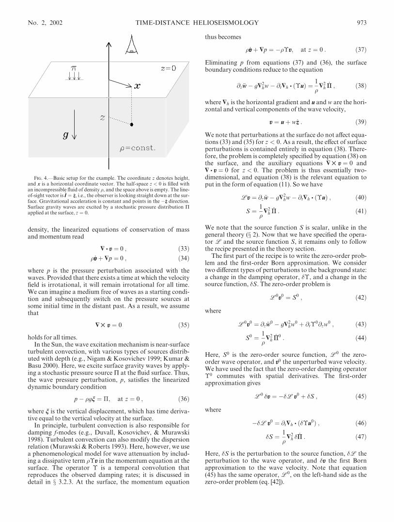
We consider a simple plane-parallel medium appropriateto studying waves with wavelengths that are small com-pared to the solar radius. The geometry is shown in Figure4. The height coordinate is z, measured upward, and a hori-zontal coordinate vector is denoted by x. Gravitationalacceleration is assumed to be constant, �gzz, where g ¼ 274m s�2 is the solar surface value. For z < 0 the fluid has a uni-form constant density, �. This assumption simplifies theproblem considerably and does not affect the dispersionrelation (!2 ¼ gk). In addition, acoustic waves are notpresent in this problem because the medium is incompressi-ble. In the steady background state there is a free surface atz ¼ 0. The background pressure distribution, PðzÞ, is hydro-static, with P ¼ ��gz.

In the following sections, we develop the equations ofmotion (x 3.2.1), encapsulated in the operator L, anddescribe our models for the source covariance (x 3.2.2) andthe wave-damping operator (x 3.2.3). We also describe thefilter F, which includes an approximation to the MDI/SOHO point-spread function (x 3.2.4). The measurementprocedure is specified by choosing the reference wavelet andthe window function (x 3.2.5).

3.2.1. Equations ofMotion

We now derive the equations of motion, which we want inthe form of equation (11). For an inviscid fluid of constant


density, the linearized equations of conservation of massandmomentum read

D

x v ¼ 0 ; ð33Þ� _vvþ

Dp ¼ 0 ; ð34Þ

where p is the pressure perturbation associated with thewaves. Provided that there exists a time at which the velocityfield is irrotational, it will remain irrotational for all time.We can imagine a medium free of waves as a starting condi-tion and subsequently switch on the pressure sources atsome initial time in the distant past. As a result, we assumethat

D

� v ¼ 0 ð35Þ

holds for all times.In the Sun, the wave excitation mechanism is near-surface

turbulent convection, with various types of sources distrib-uted with depth (e.g., Nigam & Kosovichev 1999; Kumar &Basu 2000). Here, we excite surface gravity waves by apply-ing a stochastic pressure sourceP at the fluid surface. Thus,the wave pressure perturbation, p, satisfies the linearizeddynamic boundary condition

p� �gn ¼ �; at z ¼ 0 ; ð36Þ

where n is the vertical displacement, which has time deriva-tive equal to the vertical velocity at the surface.

In principle, turbulent convection is also responsible fordamping f-modes (e.g., Duvall, Kosovichev, & Murawski1998). Turbulent convection can also modify the dispersionrelation (Murawski & Roberts 1993). Here, however, we usea phenomenological model for wave attenuation by includ-ing a dissipative term ��v in the momentum equation at thesurface. The operator � is a temporal convolution thatreproduces the observed damping rates; it is discussed indetail in x 3.2.3. At the surface, the momentum equation

thus becomes

� _vvþ

D

p ¼ ��v; at z ¼ 0 : ð37Þ

Eliminating p from equations (37) and (36), the surfaceboundary conditions reduce to the equation

@z€ww� g

D2hw� @t

D

h x ð�uÞ ¼ 1

�

D2h_�� ; ð38Þ

where

D

h is the horizontal gradient and u and w are the hori-zontal and vertical components of the wave velocity,

v ¼ uþ wzz : ð39Þ

We note that perturbations at the surface do not affect equa-tions (33) and (35) for z < 0. As a result, the effect of surfaceperturbations is contained entirely in equation (38). There-fore, the problem is completely specified by equation (38) onthe surface, and the auxiliary equations

D

� v ¼ 0 andD

x v ¼ 0 for z < 0. The problem is thus essentially two-dimensional, and equation (38) is the relevant equation toput in the form of equation (11). So we have

Lv ¼ @z€ww� g

D2hw� @t

D

h x ð�uÞ ; ð40Þ

S ¼ 1

�

D2h_�� : ð41Þ

We note that the source function S is scalar, unlike in thegeneral theory (x 2). Now that we have specified the opera-tor L and the source function S, it remains only to followthe recipe presented in the theory section.

The first part of the recipe is to write the zero-order prob-lem and the first-order Born approximation. We considertwo different types of perturbations to the background state:a change in the damping operator, ��, and a change in thesource function, �S. The zero-order problem is

L0v0 ¼ S0 ; ð42Þ

where

L0v0 ¼ @z€ww0 � g

D2hw

0 þ @t�0@zw

0 ; ð43Þ

S0 ¼ 1

�

D2h_��0 : ð44Þ

Here, S0 is the zero-order source function, L0 the zero-order wave operator, and v0 the unperturbed wave velocity.We have used the fact that the zero-order damping operator�0 commutes with spatial derivatives. The first-orderapproximation gives

L0 �v ¼ ��L v0 þ �S ; ð45Þ

where

��L v0 ¼ @t

D

h x ð��u0Þ ; ð46Þ

�S ¼ 1

�

D2h � _�� : ð47Þ

Here, �S is the perturbation to the source function, �L theperturbation to the wave operator, and �v the first Bornapproximation to the wave velocity. Note that equation(45) has the same operator, L0, on the left-hand side as thezero-order problem (eq. [42]).

Fig. 4.—Basic setup for the example. The coordinate z denotes height,and x is a horizontal coordinate vector. The half-space z < 0 is filled withan incompressible fluid of density �, and the space above is empty. The line-of-sight vector is ll ¼ zz, i.e., the observer is looking straight down at the sur-face. Gravitational acceleration is constant and points in the �zz direction.Surface gravity waves are excited by a stochastic pressure distribution Papplied at the surface, z ¼ 0.


3.2.2. Source Covariance

In order to model the zero-order covariance M0 of thesource function S0, which is necessary to compute the cross-correlation, we introduce the covariance of the applied sur-face pressure distribution�0,

�2m0ðx; t; x0; t0Þ ¼ E �0ðx; tÞ�0ðx0; t0Þ� �

; ð48Þ

which is a physical quantity. In terms of m0, the zero-ordersource covarianceM0 is given by

M0ðx; t; x0; t0Þ ¼

D2x

D2x0 @t @t0 m

0ðx; t; x0; t0Þ ; ð49Þ

where

D2x denotes the horizontal Laplacian with respect to

the variable x. Guided by the observations of Title et al.(1989), we write m0 as a product of spatial and temporaldecaying exponentials. Under the assumption of translationinvariance (in time and space),

m0ðx; t; x0; t0Þ ¼ ae�kx�x0k=Ls

2�L2s

e�jt�t0j=Ts

2Ts: ð50Þ

Here Ls is the correlation length and Ts the correlation timeof the lowest order turbulent pressure fieldP0. The constanta is the overall amplitude of m0. The normalization factors2�L2

s and 2Ts are included so that in the limits of Ls ! 0and Ts ! 0, m0 becomes the product of two Dirac deltafunctions, �Dðx� x0Þ and �Dðt� t0Þ.

Title et al. (1989) computed the covariance function ofquiet-Sun granulation intensity and found exponentialdependence on the temporal and spatial separations, jt� t0jand x� x0k k, with correlation time 400 s and correlationlength 450 km. For this work, we take Ts ¼ 400 s andLs ¼ 0. Neglecting the source correlation length, i.e., treat-ing the sources as spatially uncorrelated, is done for the sakeof computational simplicity; it is not at all a limitation ofthe theory. The approximation of zero-correlation length isappropriate because Ls is smaller than a wavelength. Forthe form of m0 given by equation (50), and the definition ofthe Fourier transform appropriate for functions that aretranslation invariant (eq. [B4]), we obtain

m0ðk; !Þ ¼ a

ð2�Þ3½1þ ð!TsÞ2�; as Ls ! 0 ; ð51Þ

which in particular does not depend on k for spatiallyuncorrelated sources. Here, as in the rest of the paper, k isthe horizontal wavevector and ! is the angular frequency.

We now consider source perturbations. As we havealready shown, what matters for the computation of cross-correlations is not the perturbation to the source but ratherthe perturbed source covariance, �M, which can beobtained from �m through

�Mðx; t; x0; t0Þ ¼

D2x

D2x0 @t @t0 �mðx; t; x0; t0Þ : ð52Þ

Three possible types of perturbations to the source cova-riance are local changes in source correlation time, correla-tion length, and amplitude. For instance, Title et al. (1989)report different correlation times in the quiet Sun and mag-netic network. Magnetic fields affect near-surface convec-tion and thus are expected to introduce local changes in thesource strength as well. Here we consider only perturbationsto the local amplitude, a, of m, i.e., to model regions of

increased or decreased f-mode emission.We choose

�mðx; t; x0; t0Þ ¼ �aðrÞa

m0ðx; t; x0; t0Þ ; ð53Þ

with

r ¼ 12 ðxþ x0Þ : ð54Þ

Here �aðrÞ gives the local change in the amplitude of thesource covariance. We have used the assumption that thesource correlation length is small compared to the lengthscale of the spatial variation of the amplitude of the sourcefunction, to write �a as a function of only the centralposition r.

3.2.3. Damping

Theoretical descriptions of the damping of f-modes byscattering from near-surface convective turbulence exist(e.g., Duvall et al. 1998), but we elect to use a phenomeno-logical model for the sake of simplicity. It is known fromobservations that high-frequency waves are damped morestrongly than low-frequency waves (e.g., Duvall et al. 1998).As a result, we need a frequency-dependent damping rate.The easiest way to implement general frequency dependenceis through a temporal convolution (e.g., Dahlen & Tromp1998). Thus, we express the zero-order damping operator,�0, as

�0vðx; tÞ ¼ 1

2�

Z 1

�1dt0 �0ðt� t0Þ vðx; t0Þ : ð55Þ

We have assumed that damping is acting purely locally. Amore sophisticated model would presumably include a spa-tial convolution in addition to the temporal convolution.With the Fourier convention given in Appendix B, �0 canbe written as

�0vðk; !Þ ¼ �0ð!Þ vðk; !Þ ; ð56Þ

where �0ð!Þ is the temporal Fourier transform of �0ðtÞ. Inaddition, we see that the operator @t þ�0, which appears inequation (37), becomes multiplication by �i!þ �0ð!Þ inthe Fourier domain.

For the sake of simplicity, we choose the function �0ðtÞ tobe real and even in time. As a result �0ð!Þ is real and even. Anonphysical consequence of this choice is that the dampingoperator is not causal. We will see, however, in x 3.3.1, thatthe Green’s function derived using this damping operator isstill causal. A treatment of causal frequency-dependentdamping can be found in Dahlen & Tromp (1998). In orderto damp all frequencies !, the function �0ð!Þ must be posi-tive (see x 3.3.1). We will see in x 3.3.2 that �0ð!Þ is the fullfrequency width at half-maximum of the surface gravitywave power. We obtain a good fit to observed f-mode linewidths (Duvall et al. 1998) if we write �0ð!Þ in the form

�0ð!Þ ¼ �!

!�

��

; ð57Þ

with the parameters !�=2� ¼ 3 mHz, �=2� ¼ 100 lHz, and� ¼ 4:4. This fit is accurate in the range1:5 mHz < !=2� < 5 mHz. The frequency dependence ofthe damping rate is strong.

There are two basic types of perturbations to the localdamping rate: a change in the amplitude of the damping


rate, �, and a change in the exponent, �. In this paper weonly consider the former and write the perturbation to thedamping operator as

�� vðx; tÞ ¼ ��ðxÞ�

�0vðx; tÞ ; ð58Þ

where ��ðxÞ=� is the local fractional perturbation in thedamping rate.

3.2.4. Observational Filter

For this example we take the line-of-sight vector to bevertical and independent of horizontal position, ll ¼ zz. Thenin accordance with equation (2) the observable is

�ðx; tÞ ¼ F vðx; tÞ x zzf g : ð59Þ

In this example we consider only the case in which there isno spatial or temporal window function in the filter F, i.e.,we observe the wave field over an area A and a time intervalT that are both very large. Therefore, the filterF can be rep-resented by multiplication by a function Fðk; !Þ in the Four-ier domain,

�ðk; !Þ ¼ Fðk; !Þwðk; !Þ ; ð60Þ

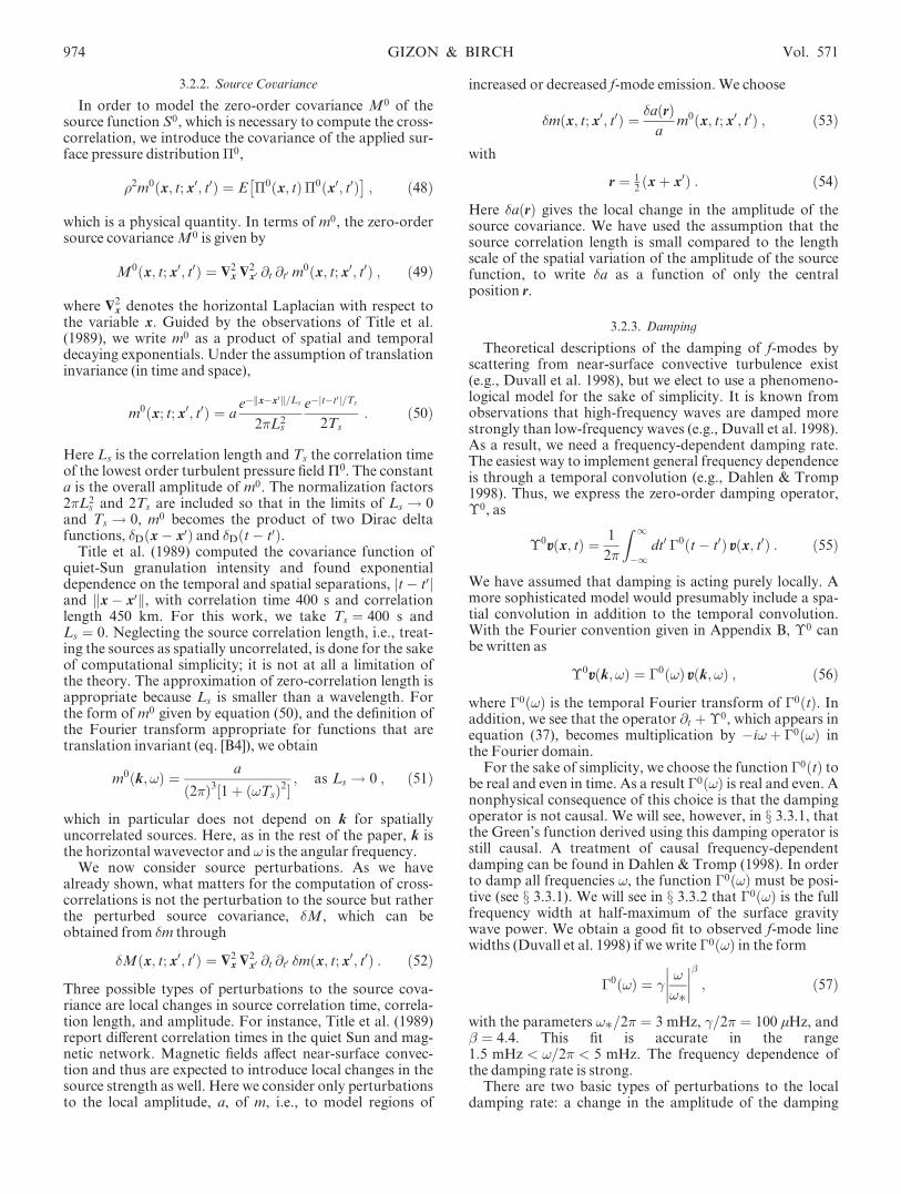
where w ¼ v x zz. The function F includes the instrumentaloptical transfer function (OTF), which is the Fourier trans-form of the point-spread function of the telescope optics, aswell as the effect of the finite pixel size of the detector. Weuse an azimuthal average of the OTF estimated by Tarbell,Acton, & Frank (1997) for the MDI/SOHO telescope in itshigh-resolution mode near disk center. We correct the OTFfor the effect of finite pixel size, , by multiplying bysincðk=2Þ, with ¼ 0:83Mm and k ¼ kk k.

In general, F also includes the filter used to select the par-ticular waves of interest in the k-! diagram and to removelow-frequency noise from the data. In this example there isonly one ridge in the k-! diagram, corresponding to the sur-face gravity waves. We choose a filter that is zero forfrequencies less than !min=2� ¼ 2 mHz and more than!max=2� ¼ 4 mHz, as was done for the data shown inFigure 1.

We include an additional factor, R, in the filter to makeour unstratified example look more solar. The functionRðkÞ is the ratio of mode inertia in our model to mode iner-tia in a standard stratified solar model:

RðkÞ ¼�R 0

�1 e2kz dzR z��1 ��ðzÞe2kz dz

: ð61Þ

Here � is the constant density in our model, and �� is thedensity as a function of height in the solar model. We usethe solar model of Christensen-Dalsgaard, Proffit, &Thompson (1993) complemented by the chromosphericmodel of Vernazza, Avrett, & Loeser (1981) up to z� ¼ 2Mm. In the solar model z ¼ 0 is the photosphere. If we hadstarted from the full stratified solar problem we would pre-sumably obtain a solar-like power spectrum without thiscorrection factor.

To summarize, we take the filter F to be

Fðk; !Þ ¼ OTFðkÞRðkÞHeað!� !minÞHeað!max � !Þ ;ð62Þ

where ‘Hea’ is the Heaviside step function. The OTF andthe k-dependence of the full filter, F, are shown in Figure 5.We repeat that we have not included the effect of an obser-vational time window, nor the effect of observing a finitearea on the Sun. Both of these effects could be included,although the filter could no longer be represented as a sim-ple multiplication in the Fourier domain.

3.2.5. Measurement of Travel Times

As explained in x 2.1, the observer needs to select thereference wavelet Cref and the window function f in order tomake a travel-time measurement. For this example, wechoose Cref to be the zero-order cross-correlation of themodel,

Crefð1; 2; tÞ ¼ C0ð1; 2; tÞ ; ð63Þ

and the window function f to be the Heaviside step function,

f ðtÞ ¼ HeaðtÞ : ð64Þ

For this choice of reference wavelet, the zero-order traveltimes �0� are zero (see Appendix A). The window function fis acceptable, as we have only a single skip (surface waves).Using equation (A8), we rewrite the travel-time perturba-tions �� in terms of the temporal Fourier transforms ofW� and �C:

��ð1; 2Þ ¼ 4�Re

Z 1

0

d!W��ð1; 2; !Þ �Cð1; 2; !Þ ; ð65Þ

where Re selects the real part of the expression. The real and

0 500 1000 1500 20000

0.2

0.4

0.6

0.8

1

k R

FilterOTF

Fig. 5.—Wavenumber dependence of the filter F and of the OTF for theexample calculation. Dashed line shows the azimuthal average of the OTFestimated by Tarbell et al. (1997) for the MDI/SOHO high-resolution tele-scope. The filter F is the product of the OTF and the mode-mass correctionR given by eq. (61). Note that the mode-mass correction suppresses thelow-wavenumber part of the spectrum, which gives better agreementbetween our unstratified model and a stratified solar model, for which low-wavenumber modes are difficult to excite.


imaginary parts ofW�ð!Þ form aHilbert transform pair:

W��ð1; 2; !Þ ¼ �Hilb !C0ð1; 2; !Þ½ � � i!C0ð1; 2; !Þ

4�R10 !02jC0ð1; 2; !0Þj2d!0

;

ð66Þ

where Hilb½. . .� denotes the Hilbert transform (Saff & Snider1993). Note that we used the fact that C0ðtÞ is even, as willbe shown in x 3.3.3. We now have an explicit definition ofthe travel-time perturbations ��þ and �� for our example.

The mean travel-time perturbation, ��mean, and thetravel-time difference, ��diff , can be expressed in the form ofequation (65) with weight functionsW�

meanð!Þ andW�diffð!Þ,

given by

W�mean ¼ 1

2 W�þ þW�

��

; ð67ÞW�

diff ¼ W�þ �W�

� : ð68Þ

From equation (66), and because C0ð!Þ is real, we see thatW�

meanð!Þ is real and that W�diffð!Þ is imaginary. Thus the

real part of the perturbation to the cross-correlation, �Cð!Þ,introduces a mean travel-time perturbation. The imaginarypart of �Cð!Þ causes a travel-time difference.

3.3. Zero-Order Solution

Now that the problem has been fully specified, we cancompute the Green’s function (x 3.3.1), the power spectrum(x 3.3.2), and the cross-correlation for the zero-order model(x 3.3.3). We show that the power spectrum in our exampleresembles the solar f-mode spectrum. We find that theunperturbed cross-correlation is the inverse Fourier trans-form of the power spectrum.

3.3.1. Green’s Function

Here we derive the Green’s function appropriate for solv-ing a problem of the form of equation (42). The vectorGreen’s function, Gðx; z; t; s; tsÞ, is the velocity response athorizontal coordinate x, height z, and time t to an impulsivesource in S at surface location s and time ts. In our exampleS is scalar, so we need only one vector Green’s function, andwe drop the superscript on the Green’s function, whichappeared in the general theory (eq. [16]). By definition, Gsolves the surface boundary condition

L0Gðx; z; t; s; tsÞ ¼ �Dðx� sÞ�Dðt� tsÞ at z ¼ 0 ; ð69Þ

with the additional constraints that G must be irrotationaland divergenceless in the bulk, as well as vanish as z ! �1.The Green’s function G is only a function of the horizontalspatial separation x� s, the time lag t� ts, and the observa-tion height z. Using the Fourier convention given by equa-tion (B4), the Fourier transform of the Green’s function canbe written

Gðk; !; zÞ ¼ ðikkþ zzÞekz

ð2�Þ3k gk � !2 � i!�0ð!Þ½ �; ð70Þ

where kk ¼ k=k. We remind the reader that in this examplethe wavevector k is horizontal. From the above expressionwe can see that the horizontal component of Gðk; !; zÞ is inthe direction of k and that the horizontal and vertical com-ponents are of the same magnitude and �=2 out of phase.The amplitude of the Green’s function decays exponentiallywith depth; the same result would apply for a vertically

stratified medium (Lamb 1932). At fixed wavenumber k, theGreen’s function has resonant frequencies ! ’� gkð Þ1=2�i�0=2 in the limit of small damping. We recognizethe dispersion relation for deep water waves. Since �0ð!Þ ispositive, the imaginary part of the two poles of the Green’sfunction is negative. This ensures that the Green’s functionis causal (e.g., Saff & Snider 1993). For later use, we alsointroduce another Green’s function,

G�ðk; !Þ ¼ i!k2Fðk; !ÞGzðk; !; z ¼ 0Þ ; ð71Þ

which gives the vertical velocity at the surface resulting froman impulsive source in�=�. The Green’s function Gz is the zzcomponent ofG given by equation (70).

3.3.2. Power

By definition, the power spectrum is the square of themodulus of the Fourier transform of the observable. Forconvenience, we consider the zero-order power spectrumper unit area and per unit time:

Pðk; !Þ ¼ ð2�Þ3

ATE �0ðk; !Þ

�� 2h i; ð72Þ

where A is the area and T the time interval over which thepower is computed. After a few simple manipulations, wefind that P is given by

Pðk; !Þ ¼ ð2�Þ6 G�ðk; !Þ�� 2m0ðk; !Þ : ð73Þ

None of the terms in the above equation depend on thedirection of k. In particular, m0 ¼ m0ðk; !Þ because thesources are spatially homogeneous and isotropic in thezero-order problem. In addition, the filter F is a functiononly of the wavenumber k and frequency !. Therefore, thepower spectrum is independent of the direction of k. Theterm jG�ðk; !Þj2 specifies the shape of the resonancepeaks in the power spectrum. For ! near gkð Þ1=2 we haveapproximately

Pðk; !Þ � k2F2m0

4!�

ffiffiffiffiffiffigk

p� �2

þ �0

2

�2" #�1

: ð74Þ

Thus, at fixed wavenumber, the line shape is Lorentzian,with full width at half-maximum �0ð!Þ.

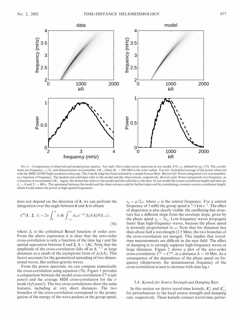
Figure 6 compares the power spectrum for our model,Pðk; !Þ, with the power spectrum for the solar f-mode ridgeobserved with the MDI/SOHO high-resolution telescope.The distribution of power with frequency and wavenumberconfirms that there is a good agreement between the modeland the observations.

3.3.3. Cross-Correlation

To obtain the zero-order cross-correlation, we use thedefinition of C0 (eq. [22]), the expression for the sourcecovariance (eq. [49]), and the definition of the Fourier trans-form to obtain

C0ð1; 2; tÞ ¼Z Z 1

�1dk

Z 1

�1d! eik xD�i!tPðk; !Þ ; ð75Þ

where D ¼ 2� 1. For the zero-order problem the cross-cor-relation is therefore the inverse Fourier transform of thepower spectrum. This is a consequence of the fact that theproblem is translation invariant. Since in our example P


does not depend on the direction of k, we can perform theintegration over the angle between k and D to obtain

C0ð1; 2; tÞ ¼ 2�

Z 1

0

k dk

Z 1

�1d! e�i!tJ0ðkDÞPðk; !Þ ;

ð76Þ

where J0 is the cylindrical Bessel function of order zero.From the above expression it is clear that the zero-ordercross-correlation is only a function of the time lag t and thespatial separation between 1 and 2, D ¼ Dk k. Note that theamplitude of the cross-correlation falls off as D�1=2 at largedistances as a result of the asymptotic form of J0ðkDÞ. Thisfactor accounts for the geometrical spreading of two-dimen-sional waves, like surface-gravity waves.

From the power spectrum, we can compute numericallythe cross-correlation using equation (76). Figure 1 providesa comparison between the model cross-correlation C0 (rightpanel) and the average MDI cross-correlation for the f-mode (left panel). The two cross-correlations show the samefeatures, including at very short distances. The twobranches of the cross-correlation correspond to the propa-gation of the energy of the wave packets at the group speed,

vg ¼ g=2!, where ! is the central frequency. For a centralfrequency of 3 mHz the group speed is 7.3 km s�1. The effectof dispersion is also clearly visible: the oscillating fine struc-ture has a different slope from the envelope slope, given bythe phase speed vp ¼ 2vg. Low-frequency waves propagatefaster than high-frequency waves, because the phase speedis inversely proportional to !. Note that for distances lessthan about half a wavelength (2.5 Mm), the two branches ofthe cross-correlation are merged. This implies that travel-time measurements are difficult in the near field. The effectof damping is to strongly suppress high-frequency waves atlarge distances. Figure 2 shows a plot of the zero-ordercross-correlation, C0 ¼ Cref , at a distance D ¼ 10Mm. As aconsequence of the dependence of the phase speed on fre-quency (dispersion), the instantaneous frequency of thecross-correlation is seen to increase with time lag t.

3.4. Kernels for Source Strength and Damping Rate

In this section we derive travel-time kernels, Ka� and K�

�,for perturbations to the local source strength and dampingrate, respectively. These kernels connect travel-time pertur-

model

kR

freq

uenc

y (m

Hz)

0 1000 20002

2.5

3

3.5

4data

kR

freq

uenc

y (m

Hz)

0 1000 20002

2.5

3

3.5

4

2 3 40

0.5

1

frequency (mHz)

Pow

er

0 1000 20000

0.5

1

kR

Pow

er

Fig. 6.—Comparison of observed and model power spectra. Top right: Zero-order power spectrum in our model, Pðk; !Þ, defined by eq. (73). The coordi-nates are frequency, !=2�, and dimensionless wavenumber, kR�, where R� ¼ 696 Mm is the solar radius. Top left: Azimuthal average of the power observedwith theMDI/SOHO high-resolution telescope. The f-mode ridge has been isolated by a simple boxcar filter. Bottom left: Power integrated over wavenumber,as a function of frequency. The dashed and solid lines refer to the model and the observations, respectively. Bottom right: Power integrated over frequency, asa function of wavenumber kR�. Again, the dotted line refers to the model and the solid line to the data. In our model the source correlation length and time areLs ¼ 0 and Ts ¼ 400 s. The agreement between the model and the observations could be further improved by considering a nonzero source correlation length,which would reduce the power at high spatial frequencies.


bations �� to fractional perturbations to the model,

��ð1; 2Þ ¼ZðAÞ

dr�aðrÞa

Ka�ð1; 2; rÞ

þZðAÞ

dr��ðrÞ�

K��ð1; 2; rÞ : ð77Þ

Here �aðrÞ=a is the local fractional change in the sourcestrength and ��ðrÞ=� the fractional change in damping rate.The two-dimensional integrals are taken over all points r onthe surface z ¼ 0, denoted by ðAÞ.

In Appendix C we give an explicit derivation of the sensi-tivity kernels K�

� and Ka�. We first compute the sensitivity of

the cross-correlation to small local changes in a and � (eqs.[C2], [C3], and [C4]). We then relate changes in the cross-correlation to changes in travel times, through the weightfunctionsW� (eq. [30]). Because of the assumptions that wehave made in this example, the kernels can be written interms of separate one-dimensional integrals over horizontalwavenumber. In Appendix C we show thatKa

� are given by

Ka�ð1; 2; rÞ ¼ 4�Re

Z 1

0

d!W��ð1; 2; !Þm0ð!Þ

� I�ðD1; !ÞIðD2; !Þ ; ð78Þ

where the integral Iðd; !Þ is a function of a distance d andfrequency ! only:

Iðd; !Þ ¼ ð2�Þ3Z 1

0

k dk J0ðkdÞG�ðk; !Þ : ð79Þ

In equation (78), D1 is the distance from 1 to r and D2 is thedistance from 2 to r. The complex integral Iðd; !Þ=ð2�Þ2 isthe spatial inverse Fourier transform of the Green’s func-tionG�ðk; !Þ.

As shown in Appendix C, the damping kernels K�� can

also be written as combinations of two one-dimensionalintegrals, IIðd; !Þ and IIIðd; !Þ:

K��ð1; 2; rÞ ¼ 4�ðDD1 x DD2ÞRe

Z 1

0

d!W��ð1; 2; !Þ

�m0ð!Þ�IIðD1; !ÞIIIðD2; !Þ

þ IIðD2; !ÞIII�ðD1; !Þ�; ð80Þ

where DD1 is a unit vector in the direction r� 1 and DD2 is aunit vector in the direction r� 2. The explicit forms of IIand III are given in Appendix C. The function III is complexand involves only one Green’s function, G�. The real inte-gral II involves two Green’s functions, Gz and G�, and isrelated to the scattering process (see Fig. 3).

We computed the kernels numerically, with grid spacingsof 7� 10�3 rad Mm�1 in k and 10�2 mHz in !=2�, whichwere selected so that the smallest line widths (1:5� 10�2 radMm�1, 1:7� 10�2 mHz) would be resolved. We ran a sec-ond set of calculations at twice the above stated resolutionsand saw only very minor changes in the resulting kernels.

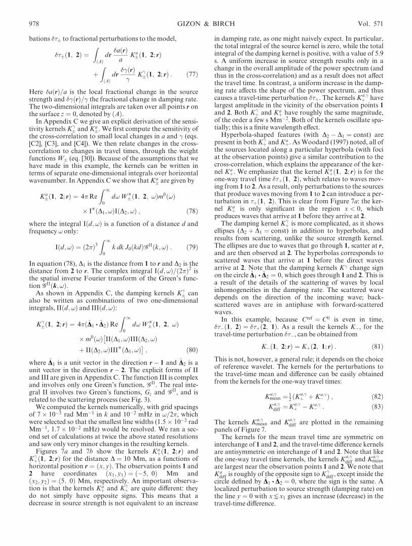
Figures 7a and 7b show the kernels Kaþð1; 2; rÞ and

K�þð1; 2; rÞ for the distance D ¼ 10 Mm, as a functions of

horizontal position r ¼ ðx; yÞ. The observation points 1 and2 have coordinates ðx1; y1Þ ¼ ð�5; 0Þ Mm andðx2; y2Þ ¼ ð5; 0Þ Mm, respectively. An important observa-tion is that the kernels Ka

þ and K�þ are quite different: they

do not simply have opposite signs. This means that adecrease in source strength is not equivalent to an increase

in damping rate, as one might naively expect. In particular,the total integral of the source kernel is zero, while the totalintegral of the damping kernel is positive, with a value of 5.9s. A uniform increase in source strength results only in achange in the overall amplitude of the power spectrum (andthus in the cross-correlation) and as a result does not affectthe travel time. In contrast, a uniform increase in the damp-ing rate affects the shape of the power spectrum, and thuscauses a travel-time perturbation ��þ. The kernels K

a;�þ have

largest amplitude in the vicinity of the observation points 1and 2. Both K

�þ and Ka

þ have roughly the same magnitude,of the order a few s Mm�2. Both of the kernels oscillate spa-tially; this is a finite wavelength effect.

Hyperbola-shaped features (with D2 � D1 ¼ const) arepresent in bothK�

þ andKaþ. AsWoodard (1997) noted, all of

the sources located along a particular hyperbola (with fociat the observation points) give a similar contribution to thecross-correlation, which explains the appearance of the ker-nel Ka

þ. We emphasize that the kernel Kaþð1; 2; rÞ is for the

one-way travel time ��þð1; 2Þ, which relates to waves mov-ing from 1 to 2. As a result, only perturbations to the sourcesthat produce waves moving from 1 to 2 can introduce a per-turbation in �þð1; 2Þ. This is clear from Figure 7a: the ker-nel Ka

þ is only significant in the region x < 0, whichproduces waves that arrive at 1 before they arrive at 2.

The damping kernel K�þ is more complicated, as it shows

ellipses (D2 þ D1 ¼ const) in addition to hyperbolas, andresults from scattering, unlike the source strength kernel.The ellipses are due to waves that go through 1, scatter at r,and are then observed at 2. The hyperbolas corresponds toscattered waves that arrive at 1 before the direct wavesarrive at 2. Note that the damping kernels K� change signon the circle DD1 x DD2 ¼ 0, which goes through 1 and 2. This isa result of the details of the scattering of waves by localinhomogeneities in the damping rate. The scattered wavedepends on the direction of the incoming wave; back-scattered waves are in antiphase with forward-scatteredwaves.

In this example, because Cref ¼ C0 is even in time,��ð1; 2Þ ¼ ��þð2; 1Þ. As a result the kernels K�, for thetravel-time perturbation ��, can be obtained from

K�ð1; 2; rÞ ¼ Kþð2; 1; rÞ : ð81Þ

This is not, however, a general rule; it depends on the choiceof reference wavelet. The kernels for the perturbations tothe travel-time mean and difference can be easily obtainedfrom the kernels for the one-way travel times:

Ka;�mean ¼ 1

2 Ka;�þ þ Ka;�

�ð Þ ; ð82ÞK

a;�diff ¼K

a;�þ � Ka;�

� : ð83Þ

The kernels Ka;�mean and Ka;�

diff are plotted in the remainingpanels of Figure 7.

The kernels for the mean travel time are symmetric oninterchange of 1 and 2, and the travel-time difference kernelsare antisymmetric on interchange of 1 and 2. Note that likethe one-way travel time kernels, the kernels K

a;�diff and K

a;�mean

are largest near the observation points 1 and 2. We note thatKa

diff is roughly of the opposite sign toK�diff , except inside the

circle defined by DD1 x DD2 ¼ 0, where the sign is the same. Alocalized perturbation to source strength (damping rate) onthe line y ¼ 0 with xdx1 gives an increase (decrease) in thetravel-time difference.


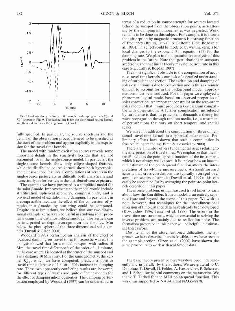
In order to show the full range of variation of the kernelswe plot, in Figure 8, cuts of the kernels Ka;�

þ along the linesy ¼ 0 and x ¼ 0. Figure 8a shows that the source kernel iszero along the line x ¼ 0, while the damping kernel is posi-tive and maximum at y ¼ 0. The side lobes (the second Fres-

nel zone) of K�þ extend out to 3.5 Mm. The slice along the

line y ¼ 0, Figure 8b, shows the complicated behavior of thekernels near the observation points, where they oscillate.

We have studied single-frequency kernels and seen thatthere is constructive interference between different fre-

Fig. 7.—Travel-time sensitivity kernels for perturbations in source strength and damping rate as functions of position r ¼ ðx; yÞ. The left column displayskernels for source strength,Ka, and the right column displays kernels for damping rate,K� . The top row gives the one-way travel-time kernelsKa;�

þ , the middlerow gives the travel-time difference kernelsKa;�

diff , and the bottom row gives the mean travel-time kernelsKa;�mean. The observation points 1 and 2 have the coordi-

nates ðx1; y1Þ ¼ ð�5; 0Þ Mm and ðx2; y2Þ ¼ ð5; 0ÞMm, respectively, and are denoted by the black crosses in each panel. The color scale indicates the localvalue of the kernel, with blue representing negative value and red positive. The color scale is truncated at�1 sMm�2. The grid spacing is 0.14Mm.


quency components along the line y ¼ 0; �1 < x < x2 forK�

þ, and the line y ¼ 0; �1 < x < x1 forKaþ. In the limit of

infinite bandwidth, the kernels K�þ and Ka

þ reduce to theserays, respectively. This is in contrast to conventional raytheory, in which the ray is restricted to the line segmenty ¼ 0; x1 < x < x2.

In the past, travel-time kernels have been calculated in the‘‘ single-source picture ’’ (Birch & Kosovichev 2000; Jensenet al. 2000). In the following section we test the single-sourcemethod by comparing single-source kernels with the kernelscalculated using a random distributed source model.

3.5. The Single-Source Picture

The single-source picture consists of placing a singlecausal source at 1 and observing the effect of local perturba-tions on the wave field observed at 2. The one-way travel-

time perturbation is approximated by the travel-time shift,

�� ssþ ð1; 2Þ ¼ �R1�1 dt ��ð2; tÞ _��0ð2; tÞR1

�1 dt ½ _��0ð2; tÞ�2; ð84Þ

between the unperturbed and perturbed signals at 2 (Birch& Kosovichev 2001). This new definition of travel time isnecessary: in the single-source picture there is no cross-cor-relation, and thus our earlier definition of travel time cannotbe used. In equation (84), �0(2) and ��(2) are the unper-turbed and perturbed wave fields at 2. The wave field is gen-erated by a causal pressure source placed at 1:

�ðs; tsÞ ¼ ��ðs� 1; tsÞ : ð85Þ

The function � characterizes the pressure source, and willlater be used to tune the source spectrum.

In this section we consider the kernel K�;ssþ , derived in the

single-source picture, which gives the sensitivity of thetravel-time perturbation ��þ to a local fractional perturba-tion in the damping rate. The single-source picture cannoteasily be used to derive a kernel for a source perturbation,which does not involve a scattering process.

By definition, the kernel K�;ssþ , which we derive in Appen-

dix D, satisfies

�� ssþ ð1; 2Þ ¼ZðAÞ

dr��ðrÞ�

K�;ssþ ð1; 2; rÞ : ð86Þ

The definition of travel time given in equation (84) closelyresembles the definition of travel time used in the generaltheory (eqs. [A6] and [A8]) if �(2, t) looks like the positivetime-lag branch of the zero-order cross-correlation from therandom source model (x 3.3.3). This condition implies thatthe spectrum of the source, �ðk; !Þ, is given by equation(D8).

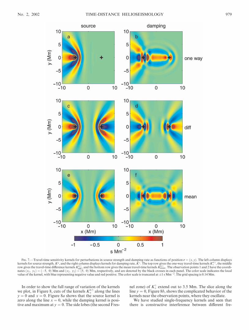
Figure 9 is a comparison of the single-source kernel K�;ssþ

with the distributed-source kernel K�þ, computed in x 3.4.

The single-source kernel fails to reproduce the hyperbola-shaped features that are seen in the random source kernel,even though the ellipses can be seen in both (with the sameorder of magnitude and sign). A single causal source at 1 isnot sufficient to generate all of the waves that are relevant tothe problem of computing travel-time kernels (see Fig. 10).

Cuts at y ¼ 0 through K�;ssþ and K�

þ are shown in Figure11, again for the distance D ¼ 10 Mm that was used in allprevious plots of kernels. The kernels agree well for xe0,where the hyperbola-shaped features in K

�þ are absent. For

xd0, the two kernels are quite different; in particular, thesingle-source kernel is nearly zero for x < �7Mm, whileK�

þhas a negative tail there.

In the limit of infinite bandwidth (ray theory), the single-source kernel K�;ss

þ would be restricted to the line segment,y ¼ 0, x1 < x < x2, in contrast to the finding (see x 3.4) thatthe distributed-source kernel K�

þ would reduce to the rayy ¼ 0,�1 < x < x2.

4. DISCUSSION

We now have a general recipe (x 2) for solving the lin-ear forward problem, i.e., computing travel-time sensitiv-ity kernels. This recipe is based on a physical descriptionof the observed wave field. The kernels give the lineardependence of travel-time perturbations on perturbations

−15 −10 −5 0 5 10 15−1

−0.8

−0.6

−0.4

−0.2

0

0.2

0.4

0.6

0.8

1s

Mm

−2

cut at x=0

a

y (Mm)

−15 −10 −5 0 5 10 15−5

−4

−3

−2

−1

0

1

2

3

4

5

s M

m−

2

cut at y=0

b

x (Mm)

Fig. 8.—Cuts through the source and damping kernels, Kaþ and K�

þ.Panel a shows cuts along the line x ¼ 0, and panel b shows cuts along theline y ¼ 0. The dashed line is for the source kernel Ka

þ, and the solid line isfor the damping kernelK�

þ.


to a solar model, and they take into account the detailsof the measurement procedure. The sensitivity kernelsdepend on the background solar model, the filtering andfitting of the data, and the position on the solar disk(through the line of sight).

In x 3 we have shown how to compute the two-dimen-sional sensitivity of travel-time perturbations to source anddamping inhomogeneities for surface gravity waves. Thisexample is important, as it shows that kernels can beobtained, using our recipe, once the physics of the model is

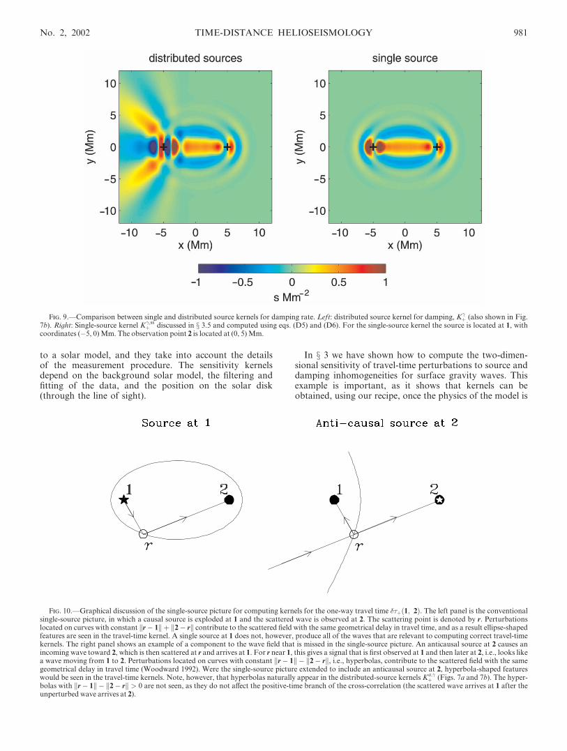
Fig. 10.—Graphical discussion of the single-source picture for computing kernels for the one-way travel time ��þð1; 2Þ. The left panel is the conventionalsingle-source picture, in which a causal source is exploded at 1 and the scattered wave is observed at 2. The scattering point is denoted by r. Perturbationslocated on curves with constant r� 1k k þ 2� rk k contribute to the scattered field with the same geometrical delay in travel time, and as a result ellipse-shapedfeatures are seen in the travel-time kernel. A single source at 1 does not, however, produce all of the waves that are relevant to computing correct travel-timekernels. The right panel shows an example of a component to the wave field that is missed in the single-source picture. An anticausal source at 2 causes anincoming wave toward 2, which is then scattered at r and arrives at 1. For r near 1, this gives a signal that is first observed at 1 and then later at 2, i.e., looks likea wave moving from 1 to 2. Perturbations located on curves with constant r� 1k k � 2� rk k, i.e., hyperbolas, contribute to the scattered field with the samegeometrical delay in travel time (Woodward 1992). Were the single-source picture extended to include an anticausal source at 2, hyperbola-shaped featureswould be seen in the travel-time kernels. Note, however, that hyperbolas naturally appear in the distributed-source kernels Ka;�

þ (Figs. 7a and 7b). The hyper-bolas with r� 1k k � 2� rk k > 0 are not seen, as they do not affect the positive-time branch of the cross-correlation (the scattered wave arrives at 1 after theunperturbed wave arrives at 2).

Fig. 9.—Comparison between single and distributed source kernels for damping rate. Left: distributed source kernel for damping, K�þ (also shown in Fig.

7b). Right: Single-source kernel K�;ssþ discussed in x 3.5 and computed using eqs. (D5) and (D6). For the single-source kernel the source is located at 1, with

coordinates (�5, 0)Mm. The observation point 2 is located at (0, 5)Mm.


fully specified. In particular, the source spectrum and thedetails of the observation procedure need to be specified atthe start of the problem and appear explicitly in the expres-sion for the travel-time kernels.

The model with random-excitation sources reveals someimportant details in the sensitivity kernels that are notaccounted for in the single-source model. In particular, thesingle-source kernels show only ellipse-shaped features,while the distributed-source kernels show both hyperbola-and ellipse-shaped features. Computations of kernels in thesingle-source picture are as difficult, both analytically andnumerically, as for kernels in the distributed-source picture.

The example we have presented is a simplified model forthe solar f-mode. Improvements to the model would includestratification, spherical geometry, compressibility, and aphysical model of excitation and damping. In particular, ina compressible medium the effect of the conversion of p-modes into f-modes by scattering could be computed.Despite these limitations, we believe that our two-dimen-sional example kernels can be useful in studying solar prob-lems using time-distance helioseismology. The kernels canbe interpreted as depth averages over the first few Mmbelow the photosphere of the three-dimensional solar ker-nels (Duvall &Gizon 2000).

Woodard (1997) performed an analysis of the effect oflocalized damping on travel times for acoustic waves; thisanalysis showed that for a model sunspot, with radius 10Mm, the travel-time difference is of the order of �1 minute,in the case where 1 is located at the center of the sunspot and2 is a distance 10Mm away. For the same geometry, the ker-nel K

�diff , which we have computed, predicts a positive

travel-time difference of 1 s for a 50% increase in dampingrate. These two apparently conflicting results are, however,for different types of waves and quite different models forthe effect of damping inhomogeneities. The damping pertur-bation employed by Woodard (1997) can be understood in

terms of a reduction in source strength for sources locatedbehind the sunspot from the observation points, as scatter-ing by the damping inhomogeneities was neglected. Workremains to be done on this subject. For example, it is knownthat absorption by magnetic structures is a strong functionof frequency (Braun, Duvall, & LaBonte 1988; Bogdan etal. 1993). This effect could be modeled by writing kernels forlocal changes to the exponent � in equation (57) for thedamping rate. We plan to do a quantitative analysis of thisproblem in the future. Note that perturbations in sunspotsare strong and that linear theory may not be accurate in thiscase (e.g., Cally & Bogdan 1997)

The most significant obstacle to the computation of accu-rate travel-time kernels is our lack of a detailed understand-ing of turbulent convection. The excitation and damping ofsolar oscillations is due to convection and is thus extremelydifficult to account for in the background model; approxi-mations must be introduced. For this paper we employed aphenomenological model based on observed properties ofsolar convection. An important constraint on the zero-ordersolar model is that it must produce a k-! diagram compati-ble with observations. A further complication introducedby turbulence is that, in principle, it demands a theory forwave propagation through random media, i.e., a treatmentof perturbations that vary on short temporal and spatialscales.

We have not addressed the computation of three-dimen-sional travel-time kernels in a spherical solar model. Pre-liminary efforts have shown that such a computation isfeasible, but demanding (Birch &Kosovichev 2000).

There are a number of less fundamental issues relating tothe interpretation of travel times. We emphasize that the fil-ter F includes the point-spread function of the instrument,which is not always well known. It is unclear how an inaccu-rate estimate of the point-spread function affects the inter-pretation of travel-time measurements. A straightforwardissue is that cross-correlations are typically averaged overannuli or sectors of annuli (Duvall et al. 1997); this caneasily be accounted for by averaging the point-to-point ker-nels described in this paper.

The inverse problem, using measured travel times to learnabout how the Sun differs from a model, is an entirely sepa-rate issue and beyond the scope of this paper. We wish tonote, however, that techniques for the three-dimensionalinversion of time-distance data have already been developed(Kosovichev 1996; Jensen et al. 1998). The errors in thetravel-time measurements, which are essential to solving theinverse problem, are mainly due to realization noise. Theformalism presented in this paper will be helpful in estimat-ing these errors.

Despite all of the aforementioned difficulties, the ap-proach we have described here is feasible, as we have seen inthe example section. Gizon et al. (2000) have shown thesame procedure to work with real f-mode data.

The basic theory presented here was developed independ-ently and in parallel by the authors. We are grateful to C.Donohue, T. Duvall, G. Felder, A. Kosovichev, P. Scherrer,and J. Schou for helpful comments on the manuscript. Wethank T. Tarbell for the MDI point-spread function. Thiswork was supported by NASA grant NAG5-8878.

−10 −5 0 5 10−2

−1.5

−1

−0.5

0

0.5

1

1.5

2

x (Mm)

s M

m−

2

Fig. 11.—Cuts along the line y ¼ 0 through the damping kernels K�þ and

K�;ssþ shown in Fig. 9. The dashed line is for the distributed-source kernel,

and the solid line is for the single-source kernel.


APPENDIX A

DEFINITION OF TRAVEL TIME

According to equation (5) the travel times �þð1; 2Þ and ��ð1; 2Þ are the time lags that minimize the functions

X�ð1; 2; tÞ ¼Z 1

�1dt0 f ð�t0Þ Cð1; 2; t0Þ � Crefð1; 2; t0 � tÞ

� �2: ðA1Þ

As a result, the time derivatives ofX� evaluated at �� are zero:

_XX�ð1; 2; ��Þ ¼ 0 : ðA2Þ

Note that _XX does not involve a time derivative of the observed cross-correlationC. In order to obtain the travel-time perturba-tions ��, we need to linearize around the zero-order travel times �0�, which are defined by

�0�ð1; 2Þ ¼ argmintfX 0�ð1; 2; tÞg : ðA3Þ

The functions X 0� refer to equation (A1) evaluated for C ¼ C0, where C0 is the zero-order cross-correlation in the reference

model. Linearizing equation (A2) about �� ¼ �0� gives

��ð1; 2Þ ¼ � � _XX�ð1; 2; �0�Þ€XX 0�ð1; 2; �0�Þ

: ðA4Þ

The functions � _XX� are given by

� _XX�ð1; 2; tÞ ¼ �2

Z 1

�1dt0 f ð�t0Þ _CCrefð1; 2; t0 � tÞ �Cð1; 2; t0Þ : ðA5Þ

We can then compute €XX 0ð�0�Þ by straightforward differentiation of equation (A1). The result for ��ð1; 2Þ is thus

��ð1; 2Þ ¼Z 1

�1dtW�ð1; 2; tÞ �Cð1; 2; tÞ ; ðA6Þ

with

W�ðtÞ ¼�f ð�tÞ _CCrefðt� �0�ÞR1

�1 dt0�f ð�t0ÞC0ðt0Þ€CCrefðt0 � �0�Þ � _ff ð�t0ÞCrefðt0 � �0�Þ _CCrefðt0 � �0�Þ

� : ðA7Þ

We have suppressed the spatial arguments 1 and 2 in the above equation for the sake of readability. This is the general linear-ized result for arbitrary Cref and f. The only assumption is that the perturbation to the cross-correlation is small compared tothe zero-order cross-correlation. Note that we have not written an explicit expression for �0�, which needs to be computednumerically by minimizingX 0

�ðtÞ (eq. [A3]).In the case where Cref and C0 are even in time, �0þ ¼ �0�. For the choice Cref ¼ C0, the zero-order travel times are both zero,

�0� ¼ 0. This choice is recommended if a theoretical model is available to the observer. With Cref ¼ C0, the weight functionsW� simplify to

W�ð1; 2; tÞ ¼ �f ð�tÞ _CC0ð1; 2; tÞR1�1 dt0 f ð�t0Þ½ _CC0ð1; 2; t0Þ�2

: ðA8Þ

In the example presented in x 3, we chooseCref ¼ C0 and f ðtÞ ¼ HeaðtÞ.

APPENDIX B

FOURIER CONVENTION FOR THE EXAMPLE SECTION

Given a function qðx; tÞ, of horizontal position x and time t, we employ the convention that the function qðx; tÞ and its Four-ier transform �qqðk; !Þ are related by

qðx; tÞ ¼Z Z 1

�1dk

Z 1

�1d! eikx�i!t�qqðk; !Þ ; ðB1Þ

�qqðk; !Þ ¼ 1

ð2�Þ3

Z Z 1

�1dx

Z 1

�1dt e�ikxþi!tqðx; tÞ ; ðB2Þ

where k is a two-dimensional horizontal wavevector and ! is the angular frequency. We commonly use the same symbol for qand �qq: the arguments make clear whether the function or its transform is intended. We use the notation qðk; !Þ when qðk; !Þonly depends on the magnitude of k, not its direction, for example in the filter function Fðk; !Þ. We note that for functions


qðx; tÞ that do not vanish at large xk k or jtj the Fourier transform is not defined. In particular, there is a problem for the casewhen the observable is not windowed in space or time. In such a case, qðk; !Þ is intended to mean the Fourier transform of thefunction qðx; tÞ truncated to zero for jtj > T=2 and xk k > A=�ð Þ1=2, where the time interval T and the area A are both largeand finite. This modification enables us to refer to the Fourier transform of a stationary/homogeneous random function (cf.Yaglom 1962, for a rigorous formalism).

When a function of four arguments,Qðx; t; x0; t0Þ, depends only on the separations x� x0 and t� t0 (translation invariance),we use the conventions

Qðx� x0; t� t0Þ ¼ Qðx; t; x0; t0Þ ; ðB3Þ

Qðk; !Þ ¼ 1

ð2�Þ3

Z Z 1

�1dx

Z 1

�1dt e�ikxþi!tQðx; tÞ : ðB4Þ

The above conventions are employed, in our example, for the functionsm0ðk; !Þ,Gðk; !; zÞ, andGðk; !Þ.Finally, we recall the relations Z 1

�1dt ei!t ¼ 2� �Dð!Þ ; ðB5ÞZ Z 1

�1dx e�ikx ¼ ð2�Þ2 �DðkÞ ; ðB6Þ

which are very useful in rewriting the kernels in Fourier space (Appendix C).

APPENDIX C

TRAVEL-TIME SENSITIVITY KERNELS FOR THE EXAMPLE

In this Appendix we derive surface gravity wave travel-time kernels, Ka� and K

��, for perturbations to local source strength

and damping rate, respectively. These kernels connect travel-time perturbations, ��, to perturbations to the model,

��ð1; 2Þ ¼ZðAÞ

dr�aðrÞa

Ka�ð1; 2; rÞ þ

ZðAÞ

dr��ðrÞ�

K��ð1; 2; rÞ : ðC1Þ

Here �aðrÞ=a is the local fractional change in the source strength, and ��ðrÞ=� is the local fractional change in damping rate.The spatial integral

RðAÞ dr is a two-dimensional integral taken over all points r on the surface z ¼ 0. From the theory part of

this paper (x 2), we know that in order to compute kernels we first need to write the perturbation to the cross-correlation interms of the functionsCa andC� (see eq. [29]):

�Cð1; 2; tÞ ¼ZðAÞ

dr�aðrÞa

Cað1; 2; t; rÞ þZðAÞ

dr��ðrÞ�

C�ð1; 2; t; rÞ : ðC2Þ

The general expression for �Cð1; 2; tÞ is given by equations (25), (26), and (27). In our example, however, the superscripts onthe Green’s function can be dropped, as the source S is scalar. To obtain Ca, we use equation (27) for CS and the definition ofthe source perturbation �M (eqs. [49] and [53]). After integrations by parts on the source variables in the right-hand side ofequation (27) and the change of variables r ¼ ðsþ s0Þ=2 and u ¼ s� s0, we obtain

Cað1; 2; t; rÞ ¼ 1

T

Zdt0 dts dt

0s dum

0ðu; ts � t0sÞG� 1� r� u

2; t0 � ts

� �G� 2� rþ u

2; t0 � t0s þ t

� �: ðC3Þ

The function C� is obtained from equation (26) with �L defined by equations (46) and (58). After integrations by parts on thesource variables, and a partial integration on the variable r, the result is

C�ð1; 2; t; rÞ ¼ 1

2�T

Zdt0 dt00 ds dts ds

0 dt0s d�tt�0ðt00 ��ttÞm0ðs� s0; ts � t0sÞ

D2h_GGhðr� s;�tt� tsÞ

x G�ð1� s0; t0 � t0sÞ

D

h_GGð2� r; t0 þ t� t00Þ þ G�ð2� s0; t0 þ t� t0sÞ

D

h_GGð1� r; t0 � t00Þ

h i; ðC4Þ

where Gh denotes the two horizontal components of the vector G . In the space-time domain these integrals are quite compli-cated to compute. They are, however, greatly simplified when written in terms of the Fourier transforms of the various func-tions:

Cað1; 2; t; rÞ ¼ ð2�Þ4Z

d! dk dk0 eik xD1�ik0 xD2�i!tm0�½ðkþ k0Þ=2; !�G��ðk; !ÞG�ðk0; !Þ ; ðC5Þ

C�ð1; 2; t; rÞ ¼ ð2�Þ7Z

d! dk dk0 eik xD1�ik0 xD2�i!t þ eik xD2�ik0 xD1þi!t� �

� �0ð!Þm0ðk; !ÞG�ðk; !ÞG��ðk; !Þkk x kk0G�ðk0; !Þ=k0 : ðC6Þ


We have used the definitions

G�ðk; !Þ ¼ Fðk; !ÞG�ðk; !Þ ; ðC7ÞG�ðk; !Þ ¼ i!k2Gzðk; !; z ¼ 0Þ ; ðC8Þ

and the identity Ghðk; !Þ ¼ ikkGzðk; !Þ resulting from equation (70). The Green’s function Gzðk; !Þ is the zz component of G ,given by equation (70).

With the assumption thatm0 is independent of k, the above expressions can be simplified to

Cað1; 2; !; rÞ ¼ m0ð!ÞI�ðD1; !ÞIðD2; !Þ ; ðC9ÞC�ð1; 2; !; rÞ ¼ m0ð!ÞDD1 x DD2 IIðD1; !ÞIIIðD2; !Þ þ IIðD2; !ÞIII�ðD1; !Þ

� �: ðC10Þ

The integrals I, II, and III are given by

Iðd; !Þ ¼ ð2�Þ3Z 1

0

k dk J0ðkdÞG�ðk; !Þ ; ðC11Þ

IIðd; !Þ ¼ ð2�Þ6�0ð!ÞZ 1

0

k dk J1ðkdÞG�ðk; !ÞG��ðk; !Þ ; ðC12Þ

IIIðd; !Þ ¼ ð2�Þ3Z 1

0

dk J1ðkdÞG�ðk; !Þ : ðC13Þ

The kernels for source strength and damping are then obtained from

Ka;�� ð1; 2; rÞ ¼ 4�Re

Z 1

0

d!W��ð1; 2; !ÞCa;�ð1; 2; !; rÞ ; ðC14Þ

withW��ð1; 2; !Þ given by equation (66). The kernels, in terms of the integrals I, II, and III, are reported in the main body of

the text (eqs. [78] and [80]).

APPENDIX D

SINGLE-SOURCE KERNELS FOR THE DAMPING RATE

In the single-source picture, we seek an expression for the kernel K�;ssþ that provides an integral relationship between the

one-way travel time �� ssþ (eq. [84]) and the local damping perturbation ��ðrÞ=�, i.e.,

�� ssþ ð1; 2Þ ¼ZðAÞ

dr��ðrÞ�

K�;ssþ ð1; 2; rÞ : ðD1Þ

We first rewrite the single-source definition of travel time (eq. [84]) in terms of the temporal Fourier transform of the signalobserved at point 2:

�� ssþ ð1; 2Þ ¼ �Re

R10 d! i!�0�ð2; !Þ ��ð2; !ÞR1

0 d!!2j�0ð2; !Þj2: ðD2Þ

Given the pressure source ��, located at point 1 and defined by equation (85), the zero- and first-order signals observed at 2are

�0ð2; !Þ ¼ ð2�Þ4Z 1

0

k dk J0ðkDÞG�ðk; !Þ�ðk; !Þ ; ðD3Þ

��ð2; !Þ ¼ ð2�Þ4 �0ð!ÞZðAÞ

dr��ðrÞ�

Zdk dk0 eik xD1�ik0 xD2G�ðk; !Þ�ðk; !Þ kk x kk0

G�ðk0; !Þk0

: ðD4Þ

Using equation (D2) we obtain the damping kernelK�;ssþ in the form

K�;ssþ ð1; 2; rÞ ¼

R10 d!!2j�0ð2; !Þj2K�;ss

þ ð1; 2; r;!ÞR10 d!!2j�0ð2; !Þj2

; ðD5Þ

with the functionK�;ssþ (single-frequency kernel) defined by

K�;ssþ ð1; 2; r;!Þ ¼ DD1 x DD2 Im

IVðD1; !Þ IIIðD2; !Þ!�0ð2; !Þ

� �: ðD6Þ


In the above equation, the function IV is a one-dimensional integral given by

IVðd; !Þ ¼ ð2�Þ3�0ð!ÞZ 1

0

k dk J1ðkdÞG�ðk; !Þ�ðk; !Þ ; ðD7Þ

and the function III denotes the integral already defined by equation (C13). Note from equation (D5) that the kernel K�;ssþ is a

frequency average ofK�;ssþ weighted by !2j�0ð2; !Þj2.

In order to compute the kernel we have to make a choice for the source spectrum,�ðk; !Þ. In general, this is difficult withouta priori knowledge of the zero-order cross-correlation. When comparing the definition of travel time of Appendix A with thesingle-source definition (eq. [84]), we find that a good match between the two definitions is obtained when �0 2; tð Þ looks likeHeaðtÞC0ð1; 2; tÞ. This condition is best met when

�ðk; !Þ ¼ � k Fðk; !Þm0ðk; !Þ2�0ð!Þ : ðD8Þ

Note that the filter function Fðk; !Þ appears in equation (D8). The kernel K�;ssþ , shown in Figure 9, was computed using this

choice.

REFERENCES

Birch, A. C., &Kosovichev, A. G. 2000, Sol. Phys., 192, 193———. 2001, in Helio- and Asteroseismology at the Dawn of the Millen-nium, ed. A.Wilson (ESA SP-464; Noordwijk: ESA), 187

Birch, A. C., Kosovichev, A. G., Price, G. H., & Schlottmann, R. B. 2001,ApJ, 561, L229

Bogdan, T. J. 1997, ApJ, 477, 475———. 2000, Sol. Phys., 192, 373Bogdan, T. J., Braun, D. C., & Lites, B.W. 1998, ApJ, 492, 379Bogdan, T. J., Brown, T. M., Lites, B. W., & Thomas, J. H. 1993, ApJ, 406,723

Braun, D. C., Duvall, T. L., Jr., & LaBonte, B. J. 1988, ApJ, 335, 1015Cally, P. S., & Bogdan, T. J. 1997, ApJ, 486, L67Chou, D.-Y., LaBonte, B. J., Braun, D. C., & Duvall, T. L., Jr. 1991, ApJ,372, 314

Christensen-Dalsgaard, J., Proffit, C. R., & Thompson, M. J. 1993, ApJ,403, L75

Dahlen, F. A., & Tromp, J. 1998, Theoretical Global Seismology (Prince-ton: PrincetonUniv. Press)

D’Silva, S., Duvall, T. L., Jr., Jefferies, S. M., & Harvey, J. W. 1996, ApJ,471, 1030

Duvall, T. L., Jr., D’Silva, S., Jefferies, S. M., Harvey, J. W., & Schou, J.1996, Nature, 379, 235

Duvall, T. L., Jr., &Gizon, L. 2000, Sol. Phys., 192, 177Duvall, T. L., Jr., Jefferies, S. M., Harvey, J. W., Osaki, Y., & Pomerantz,M. A. 1993a, ApJ, 410, 829

Duvall, T. L., Jr., Jefferies, S. M., Harvey, J. W., & Pomerantz, M. A.1993b, Nature, 362, 430

Duvall, T. L., Jr., Kosovichev, A. G., &Murawski, K. 1998, ApJ, 505, L55Duvall, T. L., Jr., et al. 1997, Sol. Phys., 170, 63Giles, P. M., Duvall, T. L., Jr., Scherrer, P. H., & Bogart, R. S. 1997,Nature, 390, 52

Gizon, L., & Birch, A. C. 2001, in Solar Encounter: The First Solar OrbiterWorkshop, ed. B. Battrick & H. Sawaya-Lacoste (ESA SP-493; Noord-wijk: ESA), 233

Gizon, L., Duvall, T. L., Jr., & Larsen, R. M. 2000, J. Astrophys. Astron.,21, 339

Gough, D. O. 1993, in Les Houches Session LXVII, Astrophysical FluidDynamics, ed. J.-P. Zahn & J. Zinn-Justin (Amsterdam: Elsevier), 399

Hung, S.-H., Dahlen, F. A., & Nolet, G. 2000, Geophys. J. Int., 141,175

Jensen, J. M., Jacobsen, B. H., & Christensen-Dalsgaard, J. 1998, in Struc-ture and Dynamics of the Interior of the Sun and Sun-like Stars, Vol. 2,ed. S. Korzennik &A.Wilson (ESA SP-418; Noordwijk: ESA), 635

———. 2000, Sol. Phys., 192, 231Kosovichev, A. G. 1996, ApJ, 461, L55Kosovichev, A. G., & Duvall, T. L., Jr. 1998, in SCORe’96: Solar Convec-tion and Oscillations and their Relationship, ed. F. P. Pijpers, J. Chris-tensen-Dalsgaard, & C. S. Rosenthal (Dordrecht: Kluwer), 241

Kosovichev, A. G., Duvall, T. L., Jr., & Scherrer, P. H. 2000, Sol. Phys.,192, 159

Kumar, P., & Basu, S. 2000, ApJ, 545, L65Lamb, H. 1932, Hydrodynamics (6th Ed.; NewYork: Dover)Lynden-Bell, D., &Ostriker, J. P. 1967,MNRAS, 136, 293Marquering, H., Dahlen, F. A., & Nolet, G. 1999, Geophys. J. Int., 137,805

Murawski, K., & Roberts, B. 1993, A&A, 272, 595Nigam, R., &Kosovichev, A. G. 1999, ApJ, 514, L53Saff, E. B., & Snider, A. D. 1993, Fundamentals of Complex Analysis forMathematics, Science, and Engineering (2d Ed.; Upper Saddle River:Prentice Hall)

Sakurai, J. J. 1995, Modern Quantum Mechanics (Reading: Addison-Wesley)

Scherrer, P. H., et al. 1995, Sol. Phys., 162, 129Stein, R. F. 1967, Sol. Phys., 2, 385Stein, R. F., &Nordlund, A. 2000, Sol. Phys., 192, 91Strous, L. H., Goode, P. R., & Rimmele, T. R. 2000, ApJ, 535, 1000Tarbell, T. D., Acton, D. S., & Frank Z. A. 1997, in Adaptative Optics,Vol. 13, ed. D. Hennage (Washington: OSA), 96

Title, A. M., Tarbell, T. D., Topka, K. P., Ferguson, S. H., Shine, R. A., &The SOUPTeam. 1989, ApJ, 336, 475

Tong, J., Dahlen, F. A., Nolet, G., & Marquering, H. 1998, Geophys. Res.Lett., 25, 1983

Vernazza, J. E., Avrett, E. H., & Loeser, R. 1981, ApJS, 45, 635Woodard,M. F. 1997, ApJ, 485, 890Woodward,M. J. 1992, Geophysics, 57, 15Yaglom, A.M. 1962, An Introduction to the Theory of Stationary RandomFunctions (EnglewoodCliffs: Prentice-Hall)

Zhao, L., & Jordan, T. H. 1998, Geophys. J. Int., 133, 683Zhao, J., Kosovichev, A. G., &Duvall, T. L., Jr. 2001, ApJ, 557, 384

986 GIZON & BIRCH

Documents

TIME-DISTANCE HELIOSEISMOLOGY: THE FORWARD PROBLEM