Seismicnotes.com

Time Dependent Rupture Forecast Model for New Zealand

Faults and Hikurangi Subduction Zone ABSTRACT : 1. INTRODUCTION New Zealand is located within a complex and interesting seismotectonic region where the Pacific plate obliquely converges and subducts beneath the Australian plate in the north, forming the Hikurangi subduction zone, and Australian plate converges and subducts beneath the Pacific plate in the south, forming the Puysegur subduction zone. This wrench type tectonics creates a large set of complex and diverse crustal faults within New Zealand that connect the subduction zones and accommodate the complex stress transfer between the converging plates. The 2010 national seismic hazard map, published by the New Zealand Institute of Geological and Nuclear Sciences (GNS), identifies about 541 crustal faults and subduction related sources on Hikurangi and Puysegur subduction zones as active known seismic sources. The GNS 2010 report treated the occurrences of large earthquakes (OLE) on majority of faults as Poissonian time-independent processes. Only the characteristic earthquakes on Wellington–Hutt Valley, Wairarapa, and southern Ohariu faults were treated as time dependent. For these faults, paleoseismic data was used to estimate conditional rupture probabilities. Formulating rupture probability of faults and subduction zones (RPFS) as time dependent can have strong implication on local and regional hazard footprints. The understanding of the physical processes behind strain accumulation and release in active tectonic regimes support the idea that the OLE on faults are not completely random. The earthquake history on faults play important role in shaping the likelihood of their future rupture. However, the scarcity of historic data of large earthquakes, in general, makes forecasting RPFS very uncertain and because of that many seismologists feel uncomfortable and even skeptical about using time dependent rupture forecast (TDRF) models for regional seismic hazard analysis. Recent earthquakes in New Zealand, Darfield 2011 and Kaikoura 2016, and earthquakes in other parts of the world have clearly demonstrated the dramatic social and financial impacts of large earthquakes on less known faults on the affected areas. Consequently, In recent years it has become highly desirable to explore ideas for estimating TDRF models for faults with uncertain past history. During the last two decades, great progress has been made in formulating stochastic TDRF models for faults, taking into consideration various model and parametric uncertainties. In this paper, we will discuss TDRF models for faults and subduction zones in New Zealand considering model and parametric uncertainties and will provide the impacts on regional hazards.

The occurrences of large earthquakes on faults inherently are time dependent, considering the

complex dynamics of strain accumulation and release by earthquakes in active tectonic regimes.

Formulating realistic TDRF models for faults is a challenge. Using physical models to simulate

earthquakes on faults for seismic hazard analysis is not practical due to lack of information to

constrain model parameters and model variabilities. The state of the practice is to use

stochastic and occasionally a hybrid of the stochastic and physical models to conduct TDRF

analysis. All such models are complex and include large parametric and model uncertainties. It

is important to understand, evaluate, and capture the impacts of these uncertainties in TDRF

analysis in order to reduce the potential biases in the TDRF results.

Most recent stochastic TDRP models use the Brownian Passage Time (BPT), lognormal, and/or Weibull distribution to describe the distribution of the rupture recurrence intervals of large earthquakes on faults (Matthews et al., 2002). The density distributions of these models are defined in terms of the mean recurrence interval, 𝑇𝑀 , and the coefficient of variance or aperiodicity, α, that defines the broadness of the distribution. In a typical analysis, 𝑇𝑀 is determined from the paleoseismic data and/or the historical records of large earthquakes using the maximum likelihood method. Until very recently, most modelers only considered faults with good paleoseismic data for TDRP analysis. However, the latest USGS TDRP model for California faults, UCERF3, used the concept of open-ended interval to formulate TDRP models for faults with no paleoseismic data. One of the concerns on using TDRP for faults without any paleoseismic data is that since the mean recurrence intervals are estimated using slip rates, that is determined using geodetic data and assumed magnitudes for the characteristic earthquakes, the TDRP estimates may carry large parametric uncertainties. This is certainly a concerning issue, however, the uncertainty in recurrence interval estimates, due to uncertainties in slip rates and the magnitudes of the characteristic earthquake, can be quantifies and included in the TDRP formulation. We will discuss this issue in more detail later. The aperiodicity parameter plays an important role in TDRP analysis. During the last two decades, there have been a number of studies on the scale of the aperiodicity parameter and its impact on TDRP analysis for faults in different regions. For example, Japan national seismicity model published by HERP, considers the approximate aperiodicity value of 0.22 for TDRP analysis of faults and subduction zones in Japan. However, the 2008 and 2010 USGS TDRP studies have considered mean aperiodicity of 0.5 with standard deviation of 0.2. The USGS, UCERF3, TDRP model considered a complex arrays of aperiodicity values, acknowledging the complex nature of the stochastic TDRP modeling that is fault dependent. The TD analysis in this study considers a hybrid of the stochastic and physical models. The stochastic models are used for basic TDRP formulation. The physical models are used to estimate the impacts of the Kaikoura earthquake on TDRP of regional faults. This includes estimating the Coulomb stress changes on faults due to Kaikoura earthquake and quantifying the impacts on the TDRP results using the rate-and-state and other more conventional physical models as will be described shortly. We have made a concerted effort to capture various types of parametric and

model uncertainties on TDRP formulation, the estimation of the Coulomb stress changes on faults due to Kaikoura earthquake, and the calculation of the impacts of the Coulomb stress changes on TDRP analysis. A typical TDRP analysis requires information on the mean recurrence (𝑇𝑀), aperiodicity of the distribution (α), date of the last rupture, and the duration of the time window of interest. As was stated, most often 𝑇𝑀 and α are estimated using a very limited paleoseismic and historic data using the maximum likelihood technique. There are large uncertainties in these estimates. In 2010, Mahdyiar et al. conducted a study on the TDRP of Japan Nankai trough and demonstrated that given the limited available data on the rupture history of the Nankai subduction zone, there are a range of aperiodicity and mean recurrence intervals that could produce the few historic observations. Although, from statistical point of view such finding was expected, the results made it clear that for TDRP analysis of faults there are shortcomings in using single 𝑇𝑀 and aperiodicity values. Based on that study, we developed a procedure for TDRP analysis to takes into consideration the uncertainties in 𝑇𝑀 and α that are consistent with the observed data and the stochastic models used to describe the recurrence intervals.

MODEL FORMULATION

Consider a fault with n rupture intervals ( )nTTT ....,,, 21 from historic and/or paleoseismic data.

Let us assume that the causative process can be modeled by a lognormal probability distribution, with the mean recurrence interval of 𝑇𝑀 and coefficient of variance (CV) of α. The likelihood function for these recurrence intervals can be written as

=

=n

i

MiM TTfTTl1

),|()|,(

(1)

where ),|( Mi TTf is the likelihood of observing the recurrence interval iT , given MT and .

For a lognormal distribution, the likelihood function (LF) can be written as

.))(ln(

2

1exp

*

1)|,(

12

2

=

−−

n

i

Mi

i

M

TT

TTTl

(2)

It is a common practice to use the maximum likelihood method to estimate the most likely values for 𝑇𝑀 and α. However, considering the scarcity of data on rupture history of faults and the strong nonlinear nature of time-dependent analysis, using the most likely estimates of 𝑇𝑀 and α rather than their distributions for TDRP analysis can be biased. Rather than using a single 𝑇𝑀 we use the likelihood function to formulate distributions for plausible 𝑇𝑀 for assumed values of α. We For any sample of α from the assumed distribution, the LF gives a density distribution for the mean recurrence interval compatible with the observed data and the assumed α-value. Using this distribution, we calculate the mean and variance for 𝑇𝑀 . Samples are drawn from this distribution to create different realizations of 𝑇𝑀. Using these 𝑇𝑀 samples and the assumed α-vale a series of recurrence interval density functions are created for TDRP analysis.

The likelihood of each TDRP estimate is calculated from the probability assigned to the sampled aperiodicity value 𝑝(𝛼) and the estimated probability for the sampled 𝑇𝑀 from the likelihood function, 𝑙(𝑇𝑀|𝛼). The final TDRP value is formulated as the following:

)(*)|(*),,(*2

1

2

1

pTltTpKPM

M

T

T

MpastMww =

(3)

where ),,( pastMw tTp is the TDRP for time window 𝑤 and K is a normalizing factor. This

formulation provides a practical way of capturing and incorporating the impacts of uncertainties in the mean recurrence and aperiodicity values on TDRP results that are consistent with the available data. For New Zealand, we consider three categories of sources for time dependent analysis:

• Group1: Crustal faults with paleoseismic data

• Group2: Crustal faults with no paleoseismic data

• Group3: Hikurangi subduction zone For Group1 we use the GNS paleoseismic data, Nicole et al 2012, for twenty-seven crustal faults and Berryman et al (year?) paleoseismic data for Alpine fault to formulate a TDRP model. For Group1 faults, the TDRP analysis is formulated using the likelihood function concept as was described. For Group2 faults, the TDRP is formulated using the open interval (OI) concept. The year 1840 is used as the completeness date for large-magnitude earthquakes in New Zealand. This implies that the Group2 faults did not rupture during the last 178 years, but the elapsed time since the last rupture can be much longer. The date of the last rupture is treated as a random variable with a uniform likelihood of occurrences prior to 1840. USGS UCERF3 considered a similar approach for TDRP formulation of faults without paleoseismic data. Obviously, the choice of quiescent time window QTW will impact the TDRP gain estimates. To create an unbiased TDRP model for Group2 faults, we constrain the QTW for each fault to one rupture cycle. In other words, it is assumed that the last rupture for each fault was one mean recurrence interval. This assumption limits the possible bias in TDRP results due to variation in recurrence intervals, considering that an arbitrary long QTW will cover different number of recurrence cycles for faults with difference recurrence intervals. Also, using a very long or an infinite QTW might not be reasonable since it implies that faults did not rupture over many cycles. Any QTW assumption beyond one cycle requires introducing some form of rupture likelihood function to properly account for the diminishing non-rupture probability with increasing QTW beyond mean recurrence. Considering that there are uncertainties in mean recurrence intervals for any assumed aperiodicity value, in this study the QTW is set as 84 percentiles of the mean recurrence distribution. Figure 2 shows the rupture probability gain distribution as a function of the mean recurrence rate for three renewal distributions: the Brownian Passage Time, the Lognormal, and the Weibull. The highest gain is calculated for faults with shorter recurrence intervals where the minimum QTW, i.e. 178 year time-window since 1840, becomes comparable to the faults mean recurrence interval. There are few faults with mean recurrence intervals shorter than 178 years.

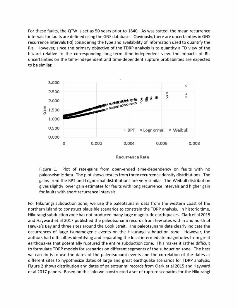
For these faults, the QTW is set as 50 years prior to 1840. As was stated, the mean recurrence intervals for faults are defined using the GNS database. Obviously, there are uncertainties in GNS recurrence intervals (RI) considering the type and availability of information used to quantify the RIs. However, since the primary objective of the TDRP analysis is to quantity a TD view of the hazard relative to the corresponding long-term time-independent view, the impacts of RIs uncertainties on the time-independent and time-dependent rupture probabilities are expected to be similar.

Figure 1. Plot of rate-gains from open-ended time-dependency on faults with no paleoseismic data. The plot shows results from three recurrence density distributions. The gains from the BPT and Lognormal distributions are very similar. The Weibull distribution gives slightly lower gain estimates for faults with long recurrence intervals and higher gain for faults with short recurrence intervals.

For Hikurangi subduction zone, we use the paleotsunami data from the western coast of the northern island to construct plausible scenarios to constrain the TDRP analysis. In historic time, Hikurangi subduction zone has not produced many large magnitude earthquakes. Clark et al 2015 and Hayward et al 2017 published the paleotsunami records from few sites within and north of Hawke’s Bay and three sites around the Cook Strait. The paleotsunami data clearly indicate the occurrences of large tsunamogenic events on the Hikurangi subduction zone. However, the authors had difficulties identifying and separating the local intermediate magnitudes from great earthquakes that potentially ruptured the entire subduction zone. This makes it rather difficult to formulate TDRP models for scenarios on different segments of the subduction zone. The best we can do is to use the dates of the paleotsunami events and the correlation of the dates at different sites to hypothesize dates of large and great earthquake scenarios for TDRP analysis. Figure 2 shows distribution and dates of paleotsunmi records from Clark et al 2015 and Hayward et al 2017 papers. Based on this info we constructed a set of rupture scenarios for the Hikurangi

subduction zone. The results of our seismicity model suggest 110, 1300, and about 10000 years of average return periods for M8, M8.5, and M9 earthquakes on Hikurangi. Note that the return period for M9 is different than what is reported in Stirling et al 2010 report. The main reason for this difference is that this model considers complete distribution for earthquakes of different magnitude, i.e. M8.0 – M9.2, for Hikurangi whereas Stirling model considered limited ranges for earthquakes and thus estimated higher rate for M9.0 type earthquakes. Hayward et al 2017 identified ten different earthquake scenarios based on the observed paleotsunami data. For TDRP analysis we used earthquakes 9(521 BP), 8(963 BP), 6(1714 BP), 4(4097 BP) and 1(7145 BP) as viable candidates that could be characterized as major earthquakes on Hikurangi. For magnitude 8, we only consider earthquake #9 which set the elapsed time of 521 years since the last rupture. Also, considering the potential rupture area of M8.0 and the fact that the Hikurangi subduction zone often is modeled as segmented, Stirling el al 2002 and 2010 and Clark el al 2015, we use 330 years return period for M8 on each of the three segments. Considering the uncertainties in the paleotsunami data and the assignments of the dates of the past earthquakes for TDRP

Impacts of the Kaikoura 2016 Earthquakes on TDRP The 2016 M7.8 Kaikoura earthquake created a complex multi-fault rupture in the north-eastern South Island. Figure 3 shows the geometry of the faults forming the Kaikoura rupture zone and the best slip distribution from inverting the geodetic and coastal deformations from Clark et al 2017. Kaikoura earthquake has altered the state of the stress on many of the local and regional faults within its reach. The state of practice for evaluating such impact is to estimate the static Coulomb stress changes (∆𝐶𝐹𝑆) on faults affected by Kaikoura to quantify the potential changes in their rupture probabilities. It should be stated that the correlation between ∆𝐶𝐹𝑆 and increase or decrease in seismic activity on faults is not yet fully established. Past observations on regional faults affected by large earthquakes worldwide have produced mixed results showing both success and failure. For this reason, we calculate the impacts of Kaikoura earthquake on regional faults, but form a logic tree to calculate TD gains for cases of considering and not considering the Kaikoura impacts to accommodate potential uncertainties. ∆𝐶𝐹𝑆 is formulated as

∆𝐶𝐹𝑆 = ∆𝜏 + 𝜇 ∗ ∆𝜎

where Δτ is the shear stress change, Δσ is the normal stress change, and µ is the effective coefficient of friction. Using the slip distribution from Clark et al 2017, we constructed a rupture model for the Kaikoura earthquake. For each fault in our model we calculate ∆CFS at a number of points along the fault length and width, Figure 3. GNS fault database is used to infer fault geometry and mechanisms in order to define the geometry of the receiver faults at each point. Considering the uncertainties in the GNS fault database, we consider 10 degrees uncertainty in dipping angles, 15 degrees uncertainty in the strikes and 30 degrees uncertainty in the rake angles. For ∆CFS analysis we use a computer program developed at AIR, based on Okada’s deformation model, for stress analysis. This program is validated against Toda’s Coulomb stress MATLAB program. The results of the analysis are mean Coulomb stress changes at selected points on faults, taking into consideration the parametric uncertainties as stated. Figure 4 shows the values at few selected sites.

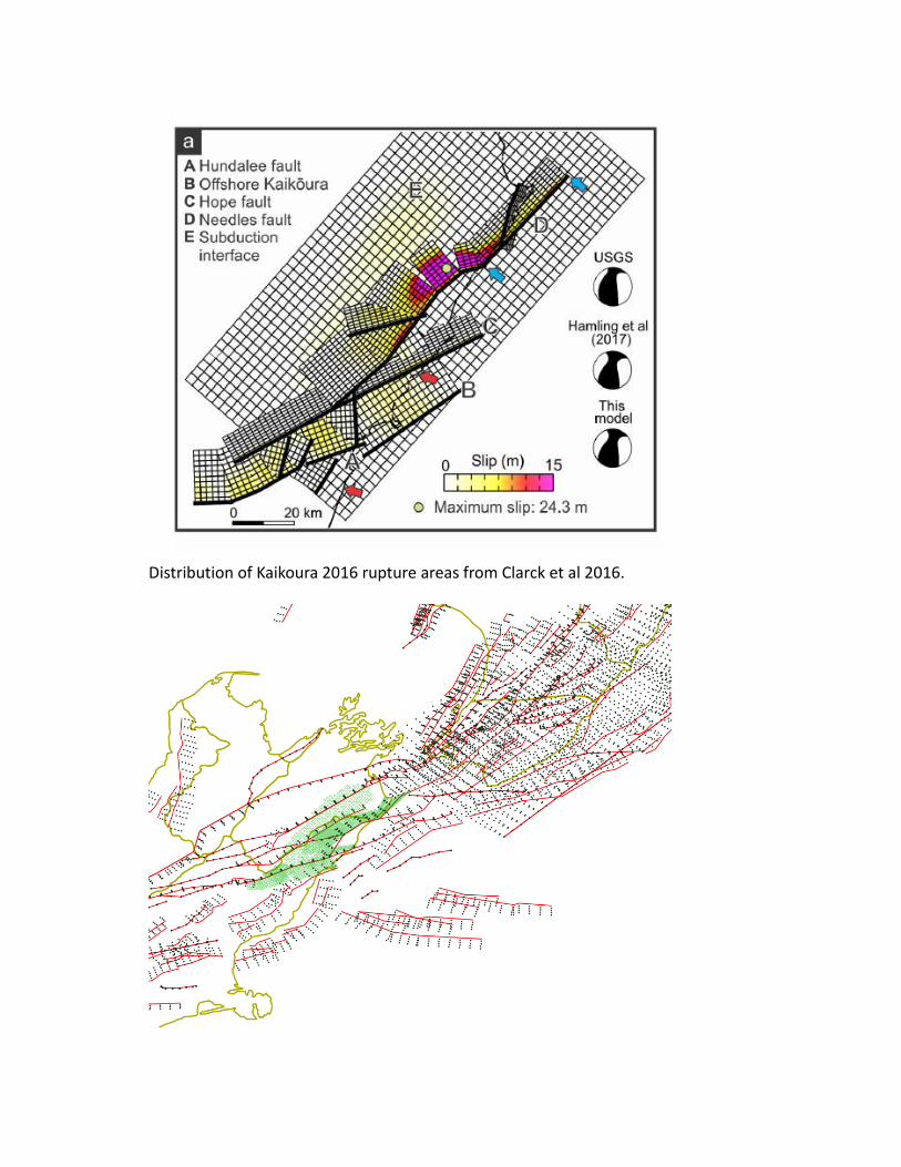
Distribution of Kaikoura 2016 rupture areas from Clarck et al 2016.

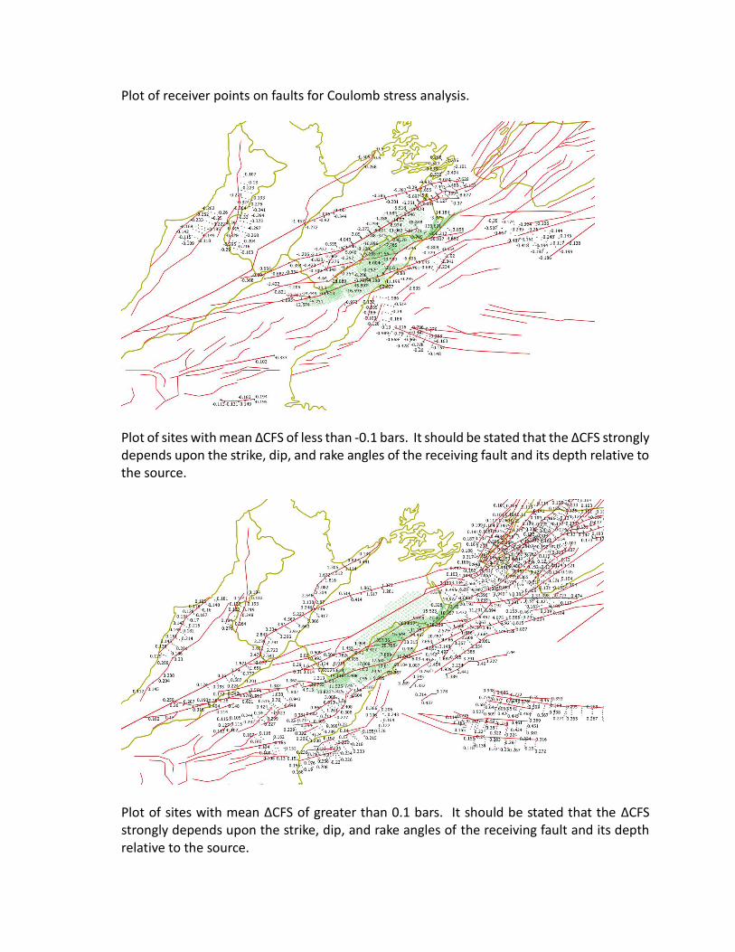
Plot of receiver points on faults for Coulomb stress analysis.

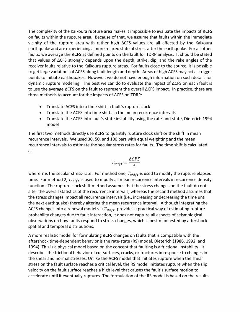
Plot of sites with mean ∆CFS of less than -0.1 bars. It should be stated that the ∆CFS strongly depends upon the strike, dip, and rake angles of the receiving fault and its depth relative to the source.

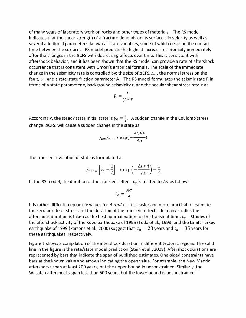
Plot of sites with mean ∆CFS of greater than 0.1 bars. It should be stated that the ∆CFS strongly depends upon the strike, dip, and rake angles of the receiving fault and its depth relative to the source.

The complexity of the Kaikoura rupture area makes it impossible to evaluate the impacts of ∆CFS on faults within the rupture area. Because of that, we assume that faults within the immediate vicinity of the rupture area with rather high ∆CFS values are all affected by the Kaikoura earthquake and are experiencing a more relaxed state of stress after the earthquake. For all other faults, we average the ∆CFS at defined points on the fault for TDRP analysis. It should be stated that values of ∆CFS strongly depends upon the depth, strike, dip, and the rake angles of the receiver faults relative to the Kaikoura rupture areas. For faults close to the source, it is possible to get large variations of ∆CFS along fault length and depth. Areas of high ∆CFS may act as trigger points to initiate earthquakes. However, we do not have enough information on such details for dynamic rupture modeling. The best we can do to evaluate the impact of ∆CFS on each fault is to use the average ∆CFS on the fault to represent the overall ∆CFS impact. In practice, there are three methods to account for the impacts of ∆CFS on TDRP:

• Translate ∆CFS into a time shift in fault’s rupture clock

• Translate the ∆CFS into time shifts in the mean recurrence intervals

• Translate the ∆CFS into fault’s state instability using the rate-and-state, Dieterich 1994 model

The first two methods directly use ∆CFS to quantify rupture clock shift or the shift in mean recurrence intervals. We used 30, 50, and 100 bars with equal weighting and the mean recurrence intervals to estimate the secular stress rates for faults. The time shift is calculated as

𝑇𝑠ℎ𝑖𝑓𝑡 =∆𝐶𝐹𝑆

�̇�

where �̇� is the secular stress-rate. For method one, 𝑇𝑠ℎ𝑖𝑓𝑡 is used to modify the rupture elapsed

time. For method 2, 𝑇𝑠ℎ𝑖𝑓𝑡 is used to modify all mean recurrence intervals in recurrence density

function. The rupture clock shift method assumes that the stress changes on the fault do not alter the overall statistics of the recurrence intervals, whereas the second method assumes that the stress changes impact all recurrence intervals (i.e., increasing or decreasing the time until the next earthquake) thereby altering the mean recurrence interval. Although integrating the ∆CFS changes into a renewal model via 𝑇𝑠ℎ𝑖𝑓𝑡 provides a practical way of estimating rupture

probability changes due to fault interaction, it does not capture all aspects of seismological observations on how faults respond to stress changes, which is best manifested by aftershock spatial and temporal distributions.

A more realistic model for formulating ∆CFS changes on faults that is compatible with the aftershock time-dependent behavior is the rate-state (RS) model, Dieterich (1986, 1992, and 1994). This is a physical model based on the concept that faulting is a frictional instability. It describes the frictional behavior of cut surfaces, cracks, or fractures in response to changes in the shear and normal stresses. Unlike the ∆CFS model that initiates rupture when the shear stress on the fault surface reaches a critical level, the RS model initiates rupture when the slip velocity on the fault surface reaches a high level that causes the fault’s surface motion to accelerate until it eventually ruptures. The formulation of the RS model is based on the results

of many years of laboratory work on rocks and other types of materials. The RS model indicates that the shear strength of a fracture depends on its surface slip velocity as well as several additional parameters, known as state variables, some of which describe the contact time between the surfaces. RS model predicts the highest increase in seismicity immediately after the changes in the ∆CFS with decreasing effects over time. This is consistent with aftershock behavior, and it has been shown that the RS model can provide a rate of aftershock occurrence that is consistent with Omori’s empirical formula. The scale of the immediate change in the seismicity rate is controlled by: the size of ∆CFS, , the normal stress on the fault, , and a rate-state friction parameter A. The RS model formulates the seismic rate R in terms of a state parameter γ, background seismicity r, and the secular shear stress rate �̇� as

𝑅 =𝑟

𝛾 ∗ �̇�

Accordingly, the steady state initial state is 𝛾0 =1

�̇�. A sudden change in the Coulomb stress

change, ∆CFS, will cause a sudden change in the state as

𝛾𝑛=𝛾𝑛−1 ∗ exp (−∆𝐶𝐹𝐹

𝐴𝜎)

The transient evolution of state is formulated as

𝛾𝑛+1= [𝛾𝑛 −1

�̇�] ∗ exp (−

∆𝑡 ∗ �̇�

𝐴𝜎) +

1

�̇�

In the RS model, the duration of the transient effect 𝑡𝑎 is related to 𝐴𝜎 as follows

𝑡𝑎 =𝐴𝜎

�̇�

It is rather difficult to quantify values for 𝐴 𝑎𝑛𝑑 𝜎. It is easier and more practical to estimate the secular rate of stress and the duration of the transient effects. In many studies the aftershock duration is taken as the best approximation for the transient time, 𝑡𝑎 . Studies of the aftershock activity of the Kobe earthquake of 1995 (Toda et al., 1998) and the Izmit, Turkey earthquake of 1999 (Parsons et al., 2000) suggest that 𝑡𝑎 = 23 years and 𝑡𝑎 = 35 years for these earthquakes, respectively.

Figure 1 shows a compilation of the aftershock duration in different tectonic regions. The solid line in the figure is the rate/state model prediction (Stein et al., 2009). Aftershock durations are represented by bars that indicate the span of published estimates. One-sided constraints have bars at the known value and arrows indicating the open value. For example, the New Madrid aftershocks span at least 200 years, but the upper bound in unconstrained. Similarly, the Wasatch aftershocks span less than 600 years, but the lower bound is unconstrained

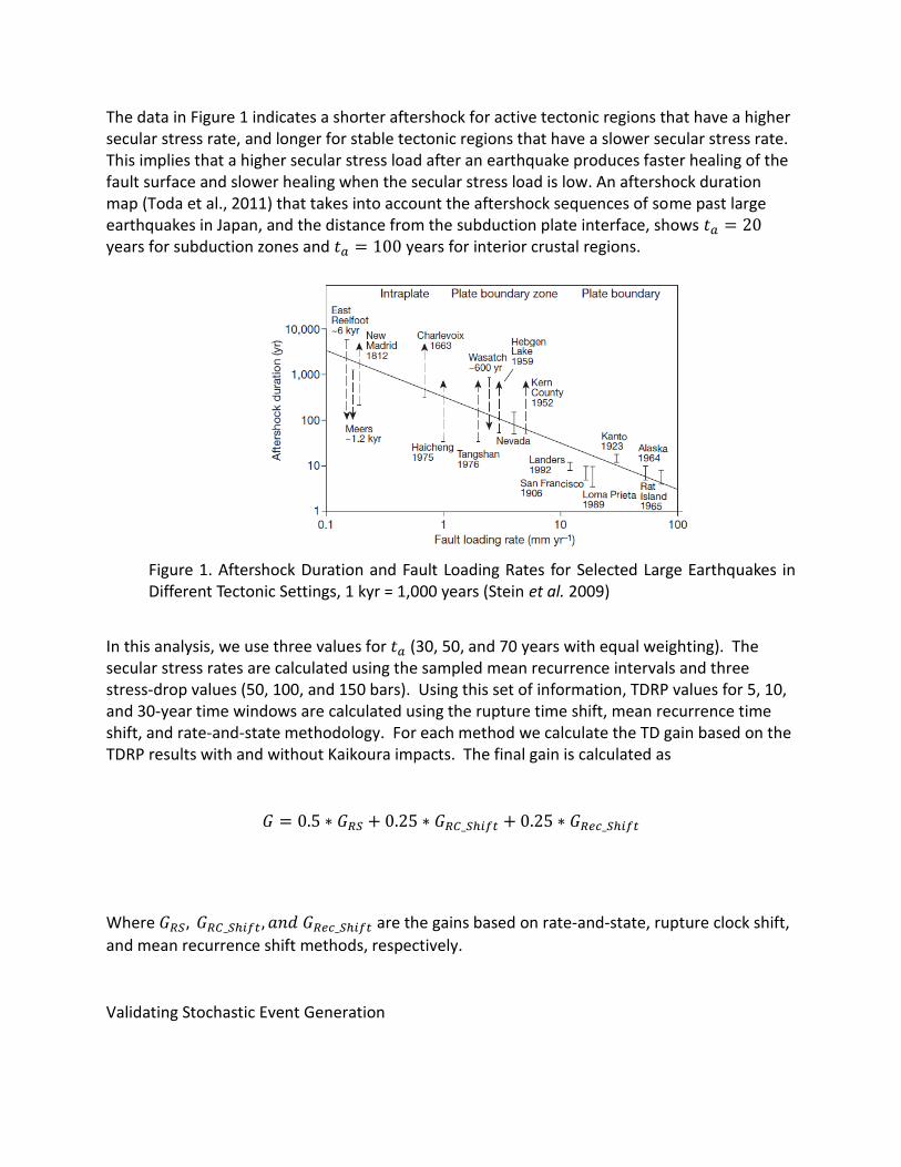
The data in Figure 1 indicates a shorter aftershock for active tectonic regions that have a higher secular stress rate, and longer for stable tectonic regions that have a slower secular stress rate. This implies that a higher secular stress load after an earthquake produces faster healing of the fault surface and slower healing when the secular stress load is low. An aftershock duration map (Toda et al., 2011) that takes into account the aftershock sequences of some past large earthquakes in Japan, and the distance from the subduction plate interface, shows 𝑡𝑎 = 20 years for subduction zones and 𝑡𝑎 = 100 years for interior crustal regions.

Figure 1. Aftershock Duration and Fault Loading Rates for Selected Large Earthquakes in Different Tectonic Settings, 1 kyr = 1,000 years (Stein et al. 2009)

In this analysis, we use three values for 𝑡𝑎 (30, 50, and 70 years with equal weighting). The secular stress rates are calculated using the sampled mean recurrence intervals and three stress-drop values (50, 100, and 150 bars). Using this set of information, TDRP values for 5, 10, and 30-year time windows are calculated using the rupture time shift, mean recurrence time shift, and rate-and-state methodology. For each method we calculate the TD gain based on the TDRP results with and without Kaikoura impacts. The final gain is calculated as

𝐺 = 0.5 ∗ 𝐺𝑅𝑆 + 0.25 ∗ 𝐺𝑅𝐶_𝑆ℎ𝑖𝑓𝑡 + 0.25 ∗ 𝐺𝑅𝑒𝑐_𝑆ℎ𝑖𝑓𝑡

Where 𝐺𝑅𝑆, 𝐺𝑅𝐶_𝑆ℎ𝑖𝑓𝑡, 𝑎𝑛𝑑 𝐺𝑅𝑒𝑐_𝑆ℎ𝑖𝑓𝑡 are the gains based on rate-and-state, rupture clock shift,

and mean recurrence shift methods, respectively.

Validating Stochastic Event Generation

As discussed in Section 1, we produce two rate based seismicity models for New Zealand. One is time-independent (TID) model with no memory of past rupture history, and another one is time-dependent (TD) model that considers historical or prehistorical ruptures to individual faults. With the rate based model, we can generate stochastic events in a given time window (e.g. in 100K-year period), and use these simulated events to validate our models with historical data. In this section, we present exhibits in magnitude frequency distribution (MFD) in selected source zones and depth profiles in several cross-sections along New Zealand.

The TDRP analyses are conducted using the lognormal, Weibull, and Brownian Passage

distribution for the recurrence intervals. Three time windows (5,10, and 30 years) are used for

the analysis. For each distribution, the probabilities are translated into their equivalent

Poissonian rates and are averaged with weighting factors of 50, 30, and 20% for 5, 10, and 30-

year time windows to estimate the average time dependent equivalent Poissonian rate

(ATDEPR) for each distribution. The final ATDEPR for each fault is calculated as

0.7 ∗ [𝐴𝑇𝐷𝐸𝑃𝑅𝐴𝐵𝑃𝑇 + 𝐴𝑇𝐷𝐸𝑃𝑅𝐴𝐿𝑜𝑔𝑛𝑜𝑟𝑚𝑎𝑙 + 𝐴𝑇𝐷𝐸𝑃𝑅𝐴𝑊𝑒𝑖𝑏𝑢𝑙𝑙] + 0.3 ∗ 𝑅𝑎𝑡𝑒𝑃𝑜𝑖𝑠𝑠𝑜𝑛

The crustal fault system recent national hazard map of Japan, released by the Headquarters for

Earthquake Promotion (HERP) in 2005 is a time-dependent model. HERP considers time-

dependent rupture probability models for most segments of the subduction zones, along with a

number of crustal faults. The Brownian Passage Time (BPT) renewal model (Matthews et al.,

2002) is used to model the stochastic inter-arrival times. To calculate the time-dependent

occurrence probability within an assumed time window, the BPT model requires information on:

the mean recurrence, aperiodicity, date of the last rupture, and the duration of the time window

of interest. HERP estimates the mean and aperiodicity parameters based on the rupture history

and the displacement of the last ruptures on faults, when such data is available, for all time-

dependent subduction zones and faults. There are uncertainties in these estimates due to the

scarcity of data on the occurrences of large historic earthquakes on subduction zones and crustal

faults. All time-dependent analyses, including the BPT, are highly nonlinear processes. This

implies that time-dependent analysis, with or without consideration of the effects of the

parametric uncertainties, will not produce the same mean conditional probability values. The

critical effects of recurrence interval uncertainty on the results of the conditional probability

analysis have been recognized and addressed by different authors. Parsons (2005) used the

Monte Carlo simulation to estimate uncertainties in the repeat times and aperiodicity values on

different segments of the San Andreas fault in southern California, and on the Nankai Trough in

Japan. Team Tokyo (Stein et al., 2006) implemented Parson’s methodology to estimate the time-

dependent probabilities for the M≥7.9 earthquake on Sagami Trough. Their estimates of the mean

recurrence and aperiodicity reflect larger uncertainty in the inter-event arrival times than those

that are used in the HERP report. Sykes and Menke [2006] used the maximum likelihood method

to estimate the uncertainty in the inter-arrival times of earthquake on a few major active faults,

and on subduction zones around the world. In general, they estimated lower level of aperiodicity

for recurrence models of several of the faults compared to other studies. These studies included

the USGS Working Group 2003 (WGCEP, 2003), which studied the time dependency of faults in

the San Francisco Bay area. Their findings suggest that the uncertainties in fault recurrence

models, for cases where the estimates of the inter-arrival times are based on historic dates, are

lower than those for which the recurrence models are dominated by the paleoseismic-related

data. However, in both cases, uncertainties in the estimates of the mean and aperiodicity values

of fault recurrence models have nonlinear effects on the results of the time-dependent

conditional probability analysis. It is important to use a systematic method of capturing such

uncertainties in order tocarry the effects through the conditional probability analysis.

2. PARAMETER SENSITIVITY OF TIME-DEPENDENT PROBABILITY CALCULATIONS

For this discussion, we use the Nankai subduction zone rupture history, and the related HERP

time-dependent model, to demonstrate the potential effects of parametric uncertainties on the

results of the time-dependent analysis. Table 1 shows the chronology of the Tonankai and the

multi-segment ruptures that included the Tokai segment of the Nankai Trough. Also shown are

the expected recurrence interval and the aperiodicity values used in the HERP report for the time-

dependent analysis. The expected recurrence interval in the HERP report for the Tonankai

segment is based on the historic data and the rupture detail information on the 1944 earthquake.

The expected recurrence for the Tokai segment is the mean of the historic rupture intervals. In

both cases, HERP uses the aperiodicity value of 0.2 for the analysis. Due to the scarcity of data,

there are uncertainties in the HERPestimates of both the recurrence and aperiodicity values.

Additionally, for the Tokai segment, there is another source of uncertainty due to the fact that the

multi-segment rupture history of the Nankai, Tonankai, and Tokai segments is used to formulate

the recurrence model for the Tokai segment. To understand the scale of uncertainty due to the

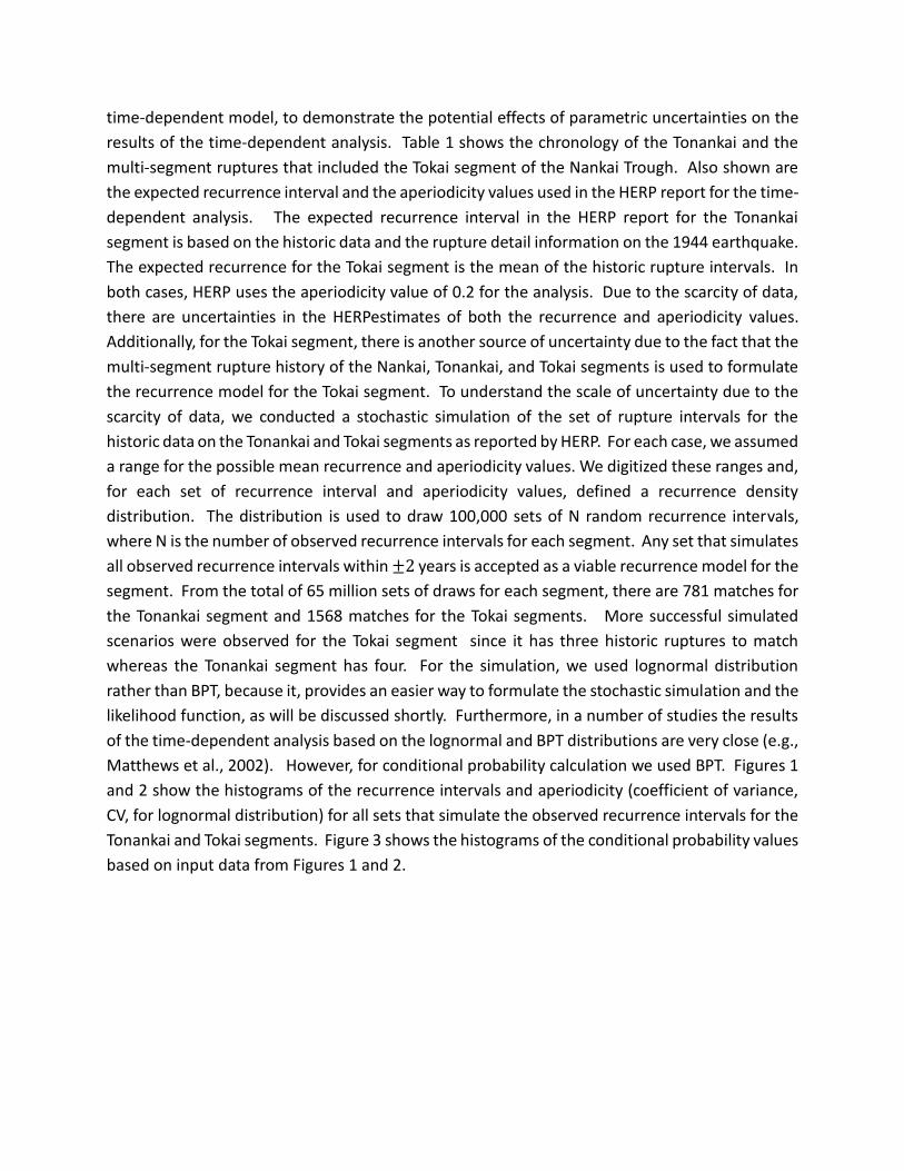
scarcity of data, we conducted a stochastic simulation of the set of rupture intervals for the

historic data on the Tonankai and Tokai segments as reported by HERP. For each case, we assumed

a range for the possible mean recurrence and aperiodicity values. We digitized these ranges and,

for each set of recurrence interval and aperiodicity values, defined a recurrence density

distribution. The distribution is used to draw 100,000 sets of N random recurrence intervals,

where N is the number of observed recurrence intervals for each segment. Any set that simulates

all observed recurrence intervals within ±2 years is accepted as a viable recurrence model for the

segment. From the total of 65 million sets of draws for each segment, there are 781 matches for

the Tonankai segment and 1568 matches for the Tokai segments. More successful simulated

scenarios were observed for the Tokai segment since it has three historic ruptures to match

whereas the Tonankai segment has four. For the simulation, we used lognormal distribution

rather than BPT, because it, provides an easier way to formulate the stochastic simulation and the

likelihood function, as will be discussed shortly. Furthermore, in a number of studies the results

of the time-dependent analysis based on the lognormal and BPT distributions are very close (e.g.,

Matthews et al., 2002). However, for conditional probability calculation we used BPT. Figures 1

and 2 show the histograms of the recurrence intervals and aperiodicity (coefficient of variance,

CV, for lognormal distribution) for all sets that simulate the observed recurrence intervals for the

Tonankai and Tokai segments. Figure 3 shows the histograms of the conditional probability values

based on input data from Figures 1 and 2.

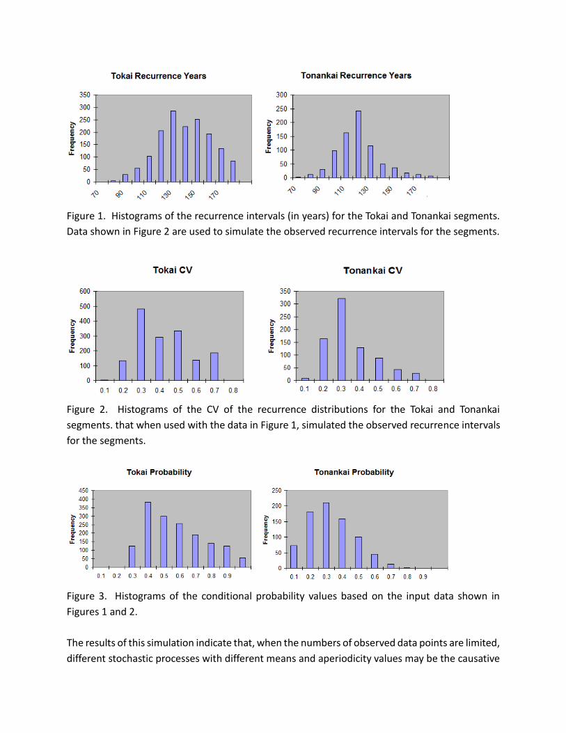
Figure 1. Histograms of the recurrence intervals (in years) for the Tokai and Tonankai segments.

Data shown in Figure 2 are used to simulate the observed recurrence intervals for the segments.

Figure 2. Histograms of the CV of the recurrence distributions for the Tokai and Tonankai

segments. that when used with the data in Figure 1, simulated the observed recurrence intervals

for the segments.

Figure 3. Histograms of the conditional probability values based on the input data shown in

Figures 1 and 2.

The results of this simulation indicate that, when the numbers of observed data points are limited,

different stochastic processes with different means and aperiodicity values may be the causative

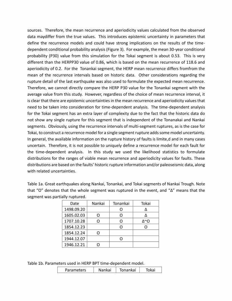
sources. Therefore, the mean recurrence and aperiodicity values calculated from the observed

data maydiffer from the true values. This introduces epistemic uncertainty in parameters that

define the recurrence models and could have strong implications on the results of the time-

dependent conditional probability analysis (Figure 3). For example, the mean 30-year conditional

probability (P30) value from this simulation for the Tokai segment is about 0.53. This is very

different than the HERPP30 value of 0.86, which is based on the mean recurrence of 118.6 and

aperiodicity of 0.2. For the Tonankai segment, the HERP mean recurrence differs fromfrom the

mean of the recurrence intervals based on historic data. Other considerations regarding the

rupture detail of the last earthquake was also used to formulate the expected mean recurrence.

Therefore, we cannot directly compare the HERP P30 value for the Tonankai segment with the

average value from this study. However, regardless of the choice of mean recurrence interval, it

is clear that there are epistemic uncertainties in the mean recurrence and aperiodicity values that

need to be taken into consideration for time-dependent analysis. The time-dependent analysis

for the Tokai segment has an extra layer of complexity due to the fact that the historic data do

not show any single rupture for this segment that is independent of the Tonanakai and Nankai

segments. Obviously, using the recurrence intervals of multi-segment ruptures, as is the case for

Tokai, to construct a recurrence model for a single segment rupture adds some model uncertainty.

In general, the available information on the rupture history of faults is limite,d and in many cases

uncertain. Therefore, it is not possible to uniquely define a recurrence model for each fault for

the time-dependent analysis. In this study we used the likelihood statistics to formulate

distributions for the ranges of viable mean recurrence and aperiodicity values for faults. These

distributions are based on the faults’ historic rupture information and/or paleoseismic data, along

with related uncertainties.

Table 1a. Great earthquakes along Nankai, Tonankai, and Tokai segments of Nankai Trough. Note

that “O” denotes that the whole segment was ruptured in the event, and “∆” means that the

segment was partially ruptured.

Date Nankai Tonankai Tokai

1498.09.20 O ∆

1605.02.03 O O ∆

1707.10.28 O O ∆~O

1854.12.23 O O

1854.12.24 O

1944.12.07 O

1946.12.21 O

Table 1b. Parameters used in HERP BPT time-dependent model.

Parameters Nankai Tonankai Tokai

Mean Recurrence

(years) 90.1 86.4 118.8

Aperiodicity 0.2 0.2 0.2

3. MODEL FORMULATION

Consider a fault with n rupture interval values ( )nttt ....,,, 21 from historic data. Let us assume

that the causative process can be modeled by a lognormal probability distribution, with the

median recurrence interval of and coefficient of variance of . The likelihood function for n

recurrence intervals can be written as

=

=n

i

itftl1

),|()|,(

(1)

where ),|( itf is the density function. For a lognormal distribution, the likelihood function

can be written as

.))(ln(

2

1exp

*

1)|,(

12

2

=

−−

n

i

i

i

t

ttl

(2)

It is common practice to use the maximum likelihood method to estimate the most likely values

for and . However, considering the scarcity of data on fault rupture history and the strong

nonlinear nature of the time-dependent analysis, using this method to obtain the most likely

estimates for and , rather than using their distributions, can introduce biases in the time-

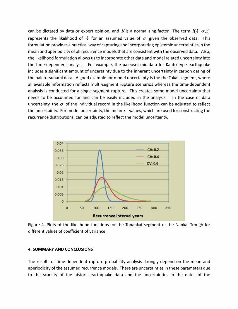
dependent probability estimates. Figure 4 shows plots of three sets of likelihood functions for

different assumed values of (CV for lognormal distribution) for the Tonankai segment. We

propose to use these distributions, with some constraints on the acceptable ranges for the

recurrence intervals and CV, to estimate the mean time-dependent occurrence probability 30P as

follows

),,(*),|( 3030

2

1

2

1

pasttptlKP

= =

=

(3)

where ),,(30 pasttp is the 30-year conditional probability. The choices for 1 , 2 , 1 , and 2

can be dictated by data or expert opinion, and K is a normalizing factor. The term ),|( tl

represents the likelihood of for an assumed value of given the observed data. This

formulation provides a practical way of capturing and incorporating epistemic uncertainties in the

mean and aperiodicity of all recurrence models that are consistent with the observed data. Also,

the likelihood formulation allows us to incorporate other data and model related uncertainty into

the time-dependent analysis. For example, the paleoseismic data for Kanto type earthquake

includes a significant amount of uncertainty due to the inherent uncertainty in carbon dating of

the paleo-tsunami data. A good example for model uncertainty is the the Tokai segment, where

all available information reflects multi-segment rupture scenarios whereas the time-dependent

analysis is conducted for a single segment rupture. This creates some model uncertainty that

needs to be accounted for and can be easily included in the analysis. In the case of data

uncertainty, the of the individual record in the likelihood function can be adjusted to reflect

the uncertainty. For model uncertainty, the mean values, which are used for constructing the

recurrence distributions, can be adjusted to reflect the model uncertainty.

Figure 4. Plots of the likelihood functions for the Tonankai segment of the Nankai Trough for

different values of coefficient of variance.

4. SUMMARY AND CONCLUSIONS

The results of time-dependent rupture probability analysis strongly depend on the mean and

aperiodicity of the assumed recurrence models. There are uncertainties in these parameters due

to the scarcity of the historic earthquake data and the uncertainties in the dates of the

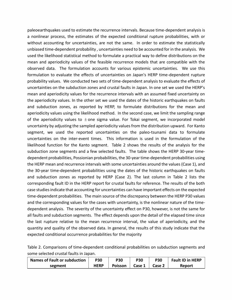
paleoearthquakes used to estimate the recurrence intervals. Because time-dependent analysis is

a nonlinear process, the estimates of the expected conditional rupture probabilities, with or

without accounting for uncertainties, are not the same. In order to estimate the statistically

unbiased time-dependent probability , uncertainties need to be accounted for in the analysis. We

used the likelihood statistical method to formulate a practical way to define distributions on the

mean and aperiodicity values of the feasible recurrence models that are compatible with the

observed data. The formulation accounts for various epistemic uncertainties. We use this

formulation to evaluate the effects of uncertainties on Japan's HERP time-dependent rupture

probability values. We conducted two sets of time-dependent analysis to evaluate the effects of

uncertainties on the subduction zones and crustal faults in Japan. In one set we used the HERP's

mean and aperiodicity values for the recurrence intervals with an assumed fixed uncertainty on

the aperiodicity values. In the other set we used the dates of the historic earthquakes on faults

and subduction zones, as reported by HERP, to formulate distributions for the mean and

aperiodicity values using the likelihood method. In the second case, we limit the sampling range

of the aperiodicity values to one sigma value. For Tokai segment, we incorporated model

uncertainty by adjusting the sampled aperiodicity values from the distribution upward. For Kanto

segment, we used the reported uncertainties on the paleo-tsunami data to formulate

uncertainties on the inter-event times. This information is used in the formulation of the

likelihood function for the Kanto segment. Table 2 shows the results of the analysis for the

subduction zone segments and a few selected faults. The table shows the HERP 30-year time-

dependent probabilities, Possionian probabilities, the 30-year time-dependent probabilities using

the HERP mean and recurrence intervals with some uncertainties around the values (Case 1), and

the 30-year time-dependent probabilities using the dates of the historic earthquakes on faults

and subduction zones as reported by HERP (Case 2). The last column in Table 2 lists the

corresponding fault ID in the HERP report for crustal faults for reference. The results of the both

case studies indicate that accounting for uncertainties can have important effects on the expected

time-dependent probabilities. The main source of the discrepancy between the HERP P30 values

and the corresponding values for the cases with uncertainty, is the nonlinear nature of the time-

dependent analysis. The severity of the uncertainty effect on P30, however, is not the same for

all faults and subduction segments. The effect depends upon the detail of the elapsed time since

the last rupture relative to the mean recurrence interval, the value of aperiodicity, and the

quantity and quality of the observed data. In general, the results of this study indicate that the

expected conditional occurrence probabilities for the majority

Table 2. Comparisons of time-dependent conditional probabilities on subduction segments and

some selected crustal faults in Japan.

Names of Fault or subduction segment

P30 HERP

P30 Poisson

P30 Case 1

P30 Case 2

Fault ID in HERP Report

Nankai segment 0.56487 0.2832 0.43739 0.18208 -

Tonankai segment 0.67385 0.29335 0.51146 0.21959 -

Tokai segment 0.87049 0.22316 0.66042 0.65466 -

Miyagi-ken-Oki 0.997 0.55453 0.96765 0.96311 -

Southern Sanriku-Oki close to trench

0.80299 0.24955 0.73599 0.67962 -

Northern Sanriku-Oki 0.04106 0.26602 0.09272 0.06649 -

Tokachi-Oki 0.00568 0.34 0.05368 0.06547 -

Nemuro-Oki 0.40132 0.34 0.43894 0.44106 -

Shikotanto-Oki 0.48093 0.34 0.48445 0.48046 -

Etorofuto-Oki 0.58483 0.34 0.5406 0.52823 -

Northwestern Hokkaido-Oki 0.00048 0.00766 0.00242 0.00243 -

Kanto segment 1923 Taisho type

0.00111 0.12747 0.02908 0.00026 -

Tobetsu fault 0.00082 0.00266 0.00142 0.00135 501

Main part- Ishikari-teichi-toen fault

0.01687 0.00623 0.01827 0.01613 601

Kuromatsunai-teichi fault zone 0.03666 0.00695 0.04927 0.0431 701

Yamagata-bonchi fault zone 0.03909 0.00995 0.04658 0.04014 1801

Shonai-heiya-toen fault zone 0.00021 0.00853 0.00137 0.00148 1901

Kushigata-sanmyaku fault zone 0.01888 0.00853 0.01678 0.01545 2501

Tsukioka fault zone 0.00022 0.00399 0.00103 0.00104 2601

Tachikawa fault zone 0.01346 0.0024 0.019 0.0166 3401

Kannawa/Kozu-Matsuda fault zone

0.04274 0.02817 0.0298 0.01032 3601

Miura-hanto fault 0.00005 0.00879 0.00106 0.00114 3701

Miura-hanto fault group 0.08378 0.017 0.09847 0.1857 3702

Itoigawa-Shizuoka-kozosen fault zone

0.14337 0.02955 0.17269 0.15209 4101

Fujikawa-kako fault zone 0.05205 0.01749 0.05595 0.04944 4301

Sanage-Takahama fault zone 0.00124 0.00283 0.00157 0.00169 5303

Kurehayama fault zone 0.00078 0.00352 0.0016 0.00155 5601

Tonami-heiya/Kurehayama fault zone

0.01149 0.00598 0.01204 0.01072 5602

Morimoto-Togashi fault zone 0.00306 0.01489 0.0065 0.00629 5701

Biwako-seigan fault zone 0.01912 0.00933 0.01997 0.01777 6501

of the subduction zone segments are reduced when compared to the corresponding HERP values.

The obvious effect of this on regional losses is that the exceedance rates of losses in the areas

dominated by large subduction-related characteristic earthquakes will decrease. The amount of

decrease on the average annual loss depends upon the overall relative contribution of these types

of earthquakes compared to those from the background and deep seismicity.

The results presented here demonstrate the importance of the epistemic uncertainty on the

mean and aperiodicity values of faults recurrence intervals in time-dependent probability

analysis. All time-dependent earthquake models suffer from lack of detailed information on

paleoseismic and historic earthquake data. It is not possible to formulate a unique recurrence

model without uncertainty. The formulation presented here is a practical way of addressing and

capturing such uncertainties by integrating the various types of data and expert opinion into a

likelihood model in order to obtain viable distributions on the mean and aperiodicity values for

time-dependent analysis.

REFERENCES Headquarters for Earthquake Research Promotion (HERP). (2005). National Seismic Hazard Maps

for Japan (2005). Http://www.jishin.go.jp/main/index-e.html.

Matthews, M. V., Ellsworth W. L., and Reasenberg P. A.. (2002). A Brownian model for recurrent

earthquakes. Bull. Seism. Soc. Am. 92 , 2233– 2250.

Parsons, T.. (2005). Significance of stress transfer in time-dependent earthquake probability

calculations. J. Geophys. Res. 110, doi:10.1029/2004JB003190.

Stein R.S., Toda S., Parsons T., and Grunewald E.. (2006). A new probabilistic seismic hazard

assessment for greater Tokyo. Phil. Trans. R. Soc. A. 364, 1965-1988.

Sykes L.R. and Menke W.. (2006). Repeat times of large earthquakes: Implications for earthquake

mechanics and long-term prediction. Bull. Seism. Soc. Am. 96:5, 1569 – 1596.

Working Group on California Earthquake Probabilities (WECEP). (2003). Earthquake

Probabilities in the San Francisco Bay Region: 2002–2031. U.S. Geological Survey, Open-File

Report 03-214.