~ 1 ~

Time-dependent Complex Vector Fields & the Drifting Vessel

John Gill January 2014

Abstract: Elementary comments on time-dependent vector fields and their contours. How does a floating vessel

drift in such a vector field? Where to place the vessel so its path ends at a certain point? Evaluating work done by

an object in a force field above the pond as it tracks the vessel. A continued fraction is interpreted as a TDVF.

Definition Zeno contour: Let , ,

( ) ( )k n k n

g z z zη ϕ= + where z S∈ and ,

( )k n

g z S∈ for a convex

set S in the complex plane. Require ,lim 0

k nn

η→∞

= , where (usually) 1,2,...,k n= . Set

1, 1,( ) ( )

n nG z g z= , ( ), , 1,

( ) ( )k n k n k n

G z g G z−= and ,

( ) ( )n n n

G z G z= with ( ) lim ( )nn

G z G z→∞

= , when

that limit exists. The Zeno contour is a graph of this iteration. The word Zeno denotes the

infinite number of actions required in a finite time period if ,k nη describes a partition of the time

interval [0,1]. Normally, ( ) ( )z f z zϕ = − for a vector field ( )=F f z , and ( , ) ( , )ϕ = −z t f z t z

for a time-dependent vector field , in which case , ,

( ) ( , )η ϕ= + ⋅ kk n k n n

g z z z .

Begin with ,

1η =

k nn

and ,

1( ) ( , )ϕ≡ + k

k n ng z z z

n with ( , )ϕ z t continuous on a domain [0,1]×S , and

,( )

k nz S g z S∈ ⇒ ∈ . (A Zeno contour forms by iteration ( )1, , , ,

: ( , )kn k n k n n k n k nnz z f z zη+ϒ = + − )

We have

31 2, 1, 2, 1,

1 1 1 1( ) ( , ) ( ( ), ) ( ( ), ) ( ( ), )ϕ ϕ ϕ ϕ −= + + + + +� n

n n n n n nn n n nG z z z G z G z G z

n n n n.

Now, imagine a function

( ) [ ] ( ) ( )1

1,

0

, , 0,1 and , lim ( ), , with , definedψ τ τ ψ ϕ ψ τ τ−→∞

∈ ≡

∫k

mk mn nm

kz z G z z d

n:

1

0

1 1 1 2 1 3 1( ) , , , , ( , )ψ ψ ψ ψ ψ τ τ

− = + + + + ≈

∫�n

nG z z z z z z z d

n n n n n n n n

And for τ irrational, ( , ) lim ( , )τ τ

ψ τ ψ τ→

=r

rz z for rational τ r .

~ 2 ~

The existence of this function (and the integral) is equivalent to the convergence of the Zeno

contour, which under appropriate conditions can be described in closed parametric form:

when

( )ϕ=dz

zdt

or ( , )dz

z tdt

ϕ= has a closed form solution, ( )z t ,

( ) (1)G z z= , (0)z z= , and ( , ) ( ( )) or ( ( ), )z t z t z t tψ ϕ ϕ= .

We begin with images of typical complex vector fields dependent upon time, t.

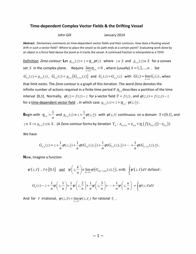
Example 1 ( , ) (( 1) ) (( 1) )f z t xCos t y iySin t x= + + + . ( ,0)f z given in dark yellow and ( ,1)f z

given in dark red. A pathline, derived as a Zeno contour, snakes its way through the plane,

describing a streamline for neither vector field.

~ 3 ~

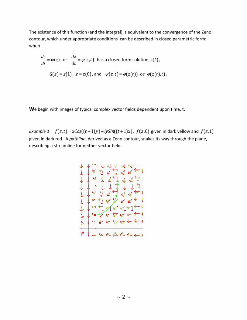
Example 2 ( , ) ztz t eϕ = or ( , ) ztf z t e z= + . One must resort to Zeno contours again. The

image of the vector field displays a panoply of twenty vectors at each point ranging from t=0

(dark green) to t=1 (light green). The contour snakes its way through the field color-coded to

match the time-determined effect at each point of time.

Parametric Contour to Time-dependent Vector Field:

Start with

(1) ( ) ( ) ( )z t x t iy t= + with : 0 1t → .

Under suitable integrability conditions the parametric form (PF) is related to a time-dependent

vector field (TDVF) as follows:

(2) ( , ) ( , )dz

z t f z t zdt

ϕ= = − for a TDVF ( , )t

f z t=F .

And ( ) ( ) ( )z t x t iy t= + is equivalent to a Zeno contour (ZC) generated by

(3) , ,( ) ( , )k

k n k n ng z z zη ϕ= + with ,

1k n

nη =

Thus , 0(1) lim ( )n n

nz G z

→∞= , 0

(0)z z=

~ 4 ~

The procedure is illustrated in

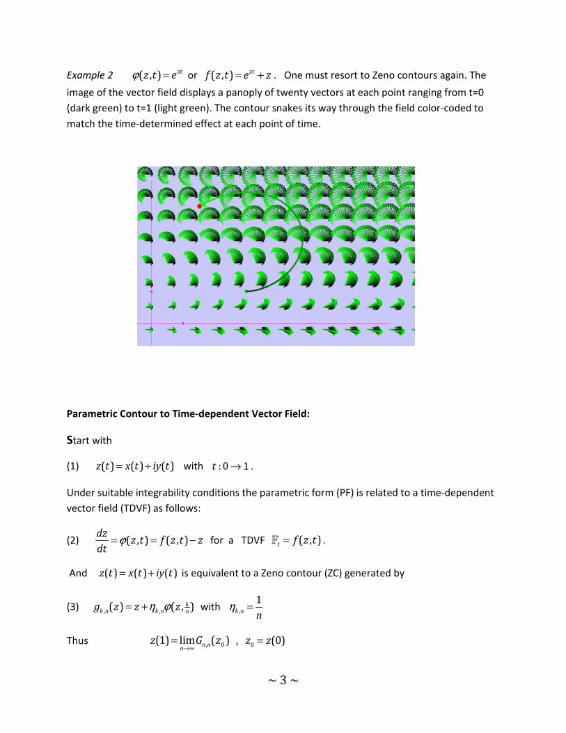
Example 3 2

0( ) ( 1)z t z t it= + + . Taking a derivative and substituting for 0(0)z z= ,

( )2

( , )1

tf z t z it

t

+ = +

+ with ( ,0) 2f z z= (green) and

3( ,1) ( )

2f z z i= + (red). 0

3z i= + .

The contours are pathlines through the TDVF, not streamlines.

Streamlines occur on regular VFs, and were they possible here, one could choose any point on

a given contour and start another contour that would coincide with the first. Clearly this cannot

happen.

When ( ) ( ) ( )z t x t iy t= + splits 0 0 0z x iy= + into real and imaginary parts a similar procedure

applies: express dz dx dy

idt dt dt

= + and deal with the two parts, as is seen in

~ 5 ~

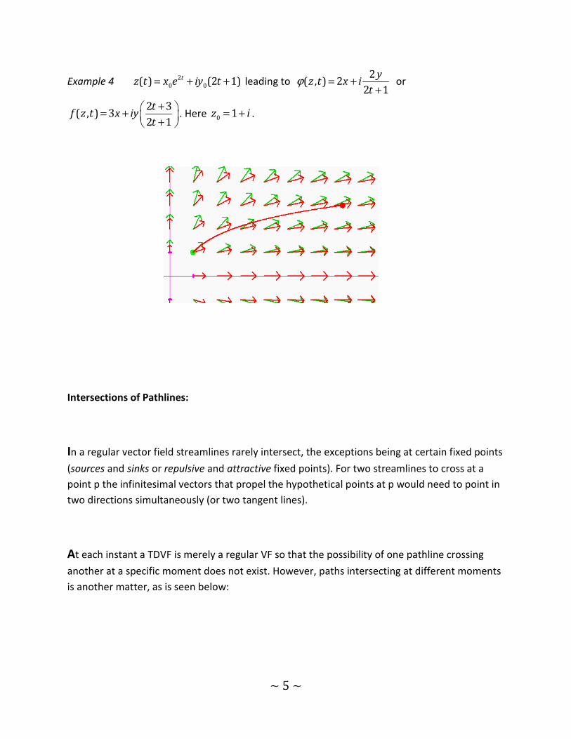
Example 4 2

0 0( ) (2 1)tz t x e iy t= + + leading to 2

( , ) 22 1

yz t x i

tϕ = +

+ or

2 3( , ) 3

2 1

tf z t x iy

t

+ = +

+ . Here 0

1z i= + .

Intersections of Pathlines:

In a regular vector field streamlines rarely intersect, the exceptions being at certain fixed points

(sources and sinks or repulsive and attractive fixed points). For two streamlines to cross at a

point p the infinitesimal vectors that propel the hypothetical points at p would need to point in

two directions simultaneously (or two tangent lines).

At each instant a TDVF is merely a regular VF so that the possibility of one pathline crossing

another at a specific moment does not exist. However, paths intersecting at different moments

is another matter, as is seen below:

~ 6 ~

Example 5 ( , ) ztf z t e z= + . Two pathlines intersect . . . but not at the same instant.

Reversing a Pathline: Drifting Vessel Problem

Think of the TDVF as the surface of a turbulent lake. Now pick a location P at random. The task

is to place a vessel at some point so that it will drift and arrive at P exactly one minute (time

unit) later. If the TDVF admits a parametric form z(t) then the task is simple: Set z(1) = P and

solve for z(0). If this is not possible the task becomes a little more difficult and requires

reversing a Zeno contour:

If ( )1, , , ,: ( , )k

n k n k n n k n k nnz z f z zη+ϒ = + − generates a Zeno contour that flows from 0

z to (1)z

then ( )1

1, , , ,: ( ,(1 ))k

n k n k n n k n k nnfω ω η ω ω−

+ϒ = − − −

Flows from 0(1)zω = to 0

(1) zω = . All under the assumption n→ ∞ .

In appearance, the contours are identical.

~ 7 ~

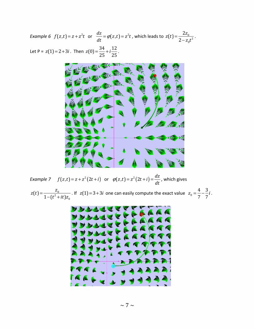
Example 6 2( , )f z t z z t= + or

2( , )dz

z t z tdt

ϕ= = , which leads to 0

2

0

2( )

2

zz t

z t=

−.

Let P = (1) 2 3z i= + . Then 34 12

(0)25 25

z i= + .

Example 7 ( )2( , ) 2f z t z z t i= + + or ( )2( , ) 2dz

z t z t idt

ϕ = + = , which gives

0

2

0

( )1 ( )

zz t

t it z=

− +. If (1) 3 3z i= + one can easily compute the exact value 0

4 3

7 7z i= − .

~ 8 ~

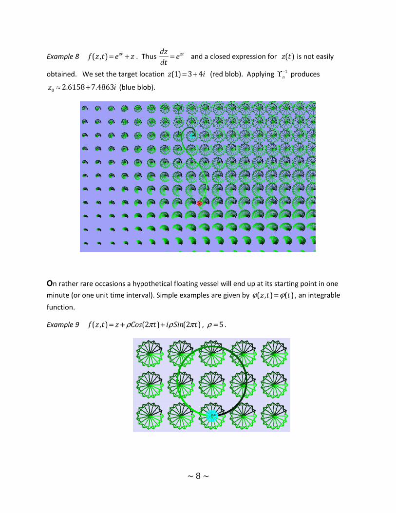
Example 8 ( , ) ztf z t e z= + . Thus ztdze

dt= and a closed expression for ( )z t is not easily

obtained. We set the target location (1) 3 4z i= + (red blob). Applying 1

n

−ϒ produces

02.6158 7.4863z i≈ + (blue blob).

On rather rare occasions a hypothetical floating vessel will end up at its starting point in one

minute (or one unit time interval). Simple examples are given by ( , ) ( )z t tϕ ϕ= , an integrable

function.

Example 9 ( , ) (2 ) (2 )f z t z Cos t i Sin tρ π ρ π= + + , 5ρ = .

~ 9 ~

The “Addition” of TDVFs:

(i) ( ), 1, , 1 1, 1,( , )k

k n k n k n k n k nnz z f z zη− − −= + − and ( ), 1, , 2 1, 1,

( , )kk n k n k n k n k nnz z f z zη− − −= + − can be

combined to produce

(ii) ( ), 1, , 1, 1,( , )k

k n k n k n k n k nnz z F z zη− − −= + − , 1 2

( , ) ( , ) ( , )F z t f z t f z t z= + − ,

which can easily be extended to more than two vector fields.

We have 1 1( , ) ( , )z t f z t zϕ = − and 2 2

( , ) ( , )z t f z t zϕ = − , with

1 2( , ) ( , ) ( , ) ( , )z t F z t z z t z tϕ ϕ ϕ= − = + .

Now it may be that 1( , )dz

z tdt

ϕ= and 2( , )dz

z tdt

ϕ= each admit simple closed solutions 1( )z t

and 2( )z t , whereas ( , )

dzz t

dtϕ= is intractable. For instance:

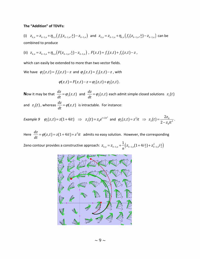
Example 9 22

1 1 0( , ) (1 4 ) ( ) t itz t z it z t z eϕ += + ⇒ = and

2 02 2 2

0

2( , ) ( )

2

zz t z it z t

z itϕ = ⇒ =

−.

Here 2( , ) (1 4 )

dzz t z it z it

dtϕ= = + + admits no easy solution. However, the corresponding

Zeno contour provides a constructive approach: ( )2

, 1, 1, 1,

1(1 4 )k k

k n k n k n k nn nz z z i z i

n− − −= + + +

~ 10 ~

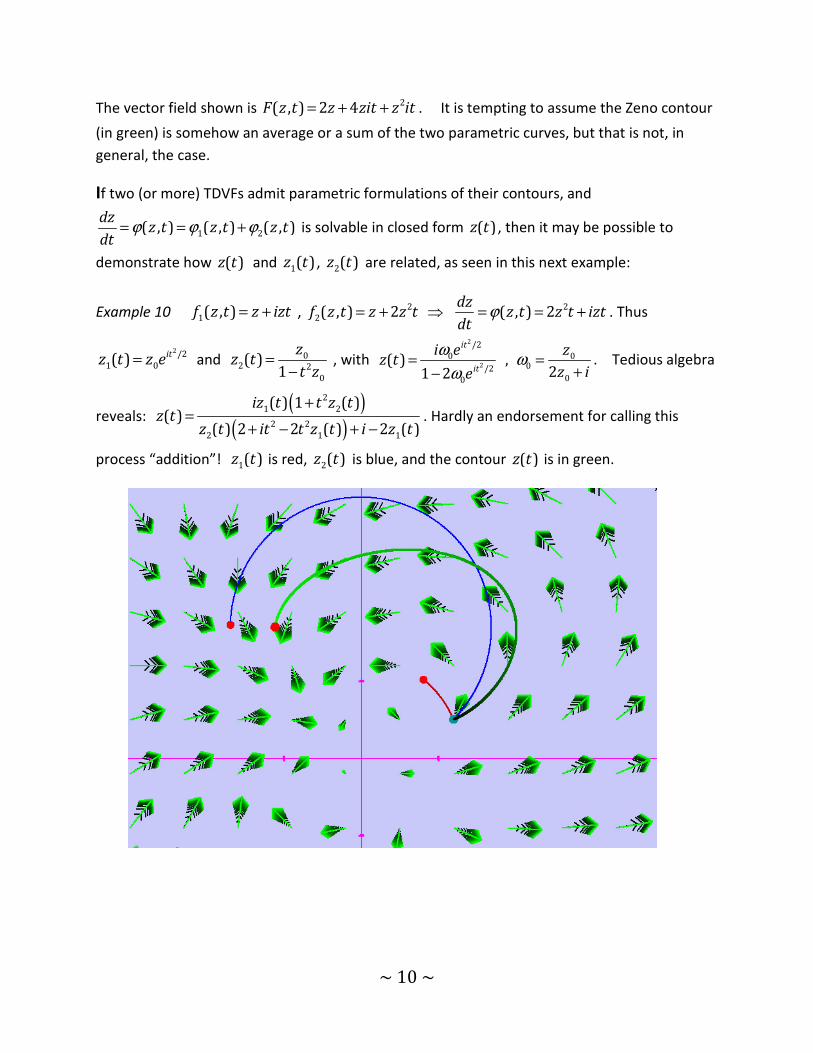
The vector field shown is 2( , ) 2 4F z t z zit z it= + + . It is tempting to assume the Zeno contour

(in green) is somehow an average or a sum of the two parametric curves, but that is not, in

general, the case.

If two (or more) TDVFs admit parametric formulations of their contours, and

1 2( , ) ( , ) ( , )dz

z t z t z tdt

ϕ ϕ ϕ= = + is solvable in closed form ( )z t , then it may be possible to

demonstrate how ( )z t and 1( )z t , 2

( )z t are related, as seen in this next example:

Example 10 1( , )f z t z izt= + ,

2

2( , ) 2f z t z z t= + ⇒ 2( , ) 2

dzz t z t izt

dtϕ= = + . Thus

2/2

1 0( ) itz t z e= and 0

2 2

0

( )1

zz t

t z=

− , with

2

2

/2

0 00/2

00

( ) , 21 2

it

it

i e zz t

z ie

ωω

ω= =

+−. Tedious algebra

reveals: ( )

( )

2

1 2

2 2

2 1 1

( ) 1 ( )( )

( ) 2 2 ( ) 2 ( )

iz t t z tz t

z t it t z t i z t

+=

+ − + −. Hardly an endorsement for calling this

process “addition”! 1( )z t is red, 2

( )z t is blue, and the contour ( )z t is in green.

~ 11 ~

Several General Categories of Vector Fields and their Contours:

The relation between a contour ( )z z t= and its vector field : ( , )f z tF has been discussed.

Here are a few simple correspondences. (0) 0α = and (0) 0β = .

(1) 0( ) ( ) ( , ) ( )z t z t f z t z tα α′= + ↔ = +

(2) ( )( )

0( ) ( , ) 1 ( )tz t z e f z t z tα α ′= ↔ = +

(3) ( ) ( )0( ) 1 ( ) ( , ) 1 ( ) ( )

1 ( )

zz t z t f z t t z t

tα α α

α′= + ↔ = + +

+

(4) ( )2

0

0

( ) ( ) ( ) ( ) ( ) ( )( )( ) ( , )

1 ( ) 1 ( ) ( )

z t z t t t t tz tz t f z t z

z t t t

β α β α β αα

β α β

′ ′ ′ ′+ − ++= ↔ = +

− +

(5) ( )2 2

0

2

0

( ) ( ) ( ) ( ) ( )( )( ) ( , )

1 ( ) ( )

z t t z t t tz tz t f z t

z t t

α β α α αα

β α

′ ′+ += ↔ =

−, (0) 1α =

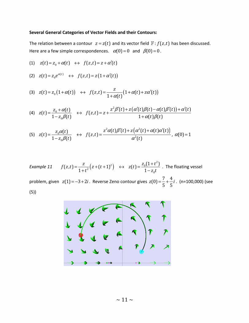
Example 11 ( )2

2 0

2

0

(1 )( , ) ( 1) ( )

1 1

z z tf z t z t z t

t z t

+= + + ↔ =

+ − . The floating vessel

problem, given (1) 3 2z i= − + . Reverse Zeno contour gives 7 4

(0)5 5

z i= + . (n=100,000) (see

(5))

~ 12 ~

Tracking the Drifting Vessel – Work done by an Object in a Force Field above the Vessel:

Assume the vessel is subject to fluid flow given by 1F and the object is subject to the force field

2F , both of which are time-dependent. The problem is the following:

(a) Choose a point in the lake where you wish the vessel to be at t=1;

(b) Locate the point where the (drifting) vessel must be at t=0 in order to achieve this;

(c) Assume the object is above the vessel at all times, tracking the vessel;

(d) Compute the work done by the object during the time interval [0,1].

Starting with 1, 1: ( , )

tf z tF and 1 1

( , ) ( , )z t f z t zϕ = − , if 1( , )dz

z tdt

ϕ= has a closed form solution

( ) ( ) ( )z t x t iy t= + then the problem may be solvable in closed form if all expressions, including

2, 2: ( , )

tf z tF , are fairly simple. However, it is highly likely an integral expression will require an

approximation. Therefore, we deal only with the general case in which all that is required is that

the various functions be continuous in all variables. The method outlined will include all

approximations in one algorithm. The procedure begins with the reverse Zeno contour

( )1

1, , 1 , ,: ( ,(1 ))k

n k n k n n k n k nnfω ω η ω ω−

+ϒ = − − − , employed to locate (1) (0)zω = for a pre-

assigned value (0) (1)zω = . Once this is done, the standard contour is generated by

( )1, , 1 , ,: ( , )k

n k n k n n k n k nnz z f z zη+ϒ = + − . Now, the work done is given by

1

2 2

0

Re ( , ) Re ( , )dz

f z t dz f z t dtdt

ϒ

=∫ ∫ which is derived from

( )2 , 1, , 2 , , ,

1( , ) ( , ) ( , )k k k

k n k n k n k n k n k nn n nf z z z f z z

nϕ σ+ − = ⋅ ≡ so that

2 ,

1

Re ( , ) lim Re( )n

k nn

k

f z t dz σ→∞

=ϒ

= ∑∫

The next example demonstrates this process in a case in which a closed form is doubtful:

~ 13 ~

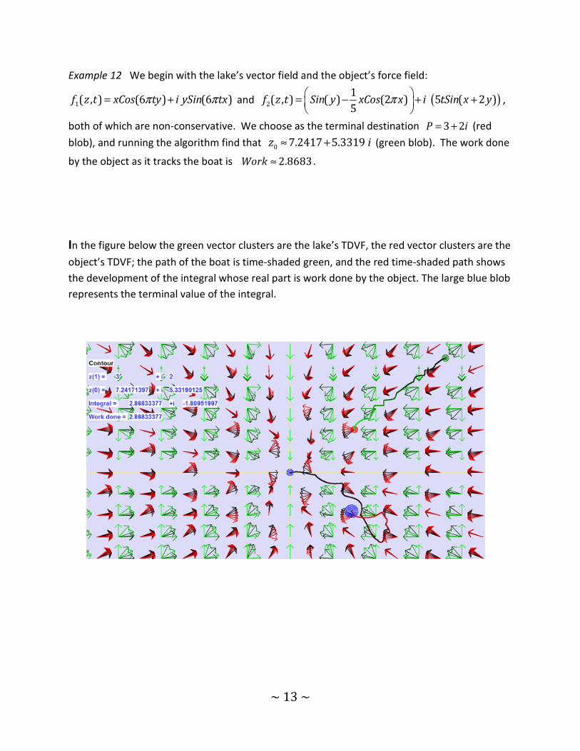
Example 12 We begin with the lake’s vector field and the object’s force field:

1( , ) (6 ) (6 )f z t xCos ty i ySin txπ π= + and ( )2

1( , ) ( ) (2 ) 5 ( 2 )

5f z t Sin y xCos x i tSin x yπ

= − + +

,

both of which are non-conservative. We choose as the terminal destination 3 2P i= + (red

blob), and running the algorithm find that 07.2417 5.3319 z i≈ + (green blob). The work done

by the object as it tracks the boat is 2.8683Work ≈ .

In the figure below the green vector clusters are the lake’s TDVF, the red vector clusters are the

object’s TDVF; the path of the boat is time-shaded green, and the red time-shaded path shows

the development of the integral whose real part is work done by the object. The large blue blob

represents the terminal value of the integral.

~ 14 ~

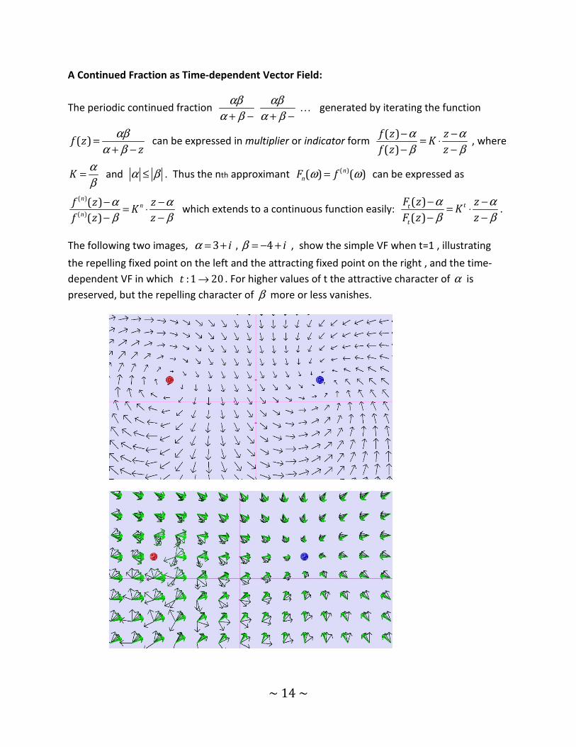
A Continued Fraction as Time-dependent Vector Field:

The periodic continued fraction αβ αβ

α β α β+ − + −… generated by iterating the function

( )f zz

αβ

α β=

+ − can be expressed in multiplier or indicator form

( )

( )

f z zK

f z z

α α

β β

− −= ⋅

− − , where

Kα

β= and α β≤ . Thus the nth approximant

( )( ) ( )n

nF fω ω= can be expressed as

( )

( )

( )

( )

nn

n

f z zK

f z z

α α

β β

− −= ⋅

− − which extends to a continuous function easily:

( )

( )

tt

t

F z zK

F z z

α α

β β

− −= ⋅

− −.

The following two images, 3 , 4i iα β= + = − + , show the simple VF when t=1 , illustrating

the repelling fixed point on the left and the attracting fixed point on the right , and the time-

dependent VF in which :1 20t → . For higher values of t the attractive character of α is

preserved, but the repelling character of β more or less vanishes.

~ 15 ~

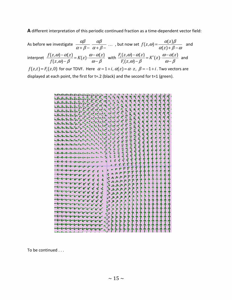
A different interpretation of this periodic continued fraction as a time-dependent vector field:

As before we investigate αβ αβ

α β α β+ − + −… , but now set

( )( , )

( )

zf z

z

α βω

α β ω=

+ − and

interpret ( , ) ( ) ( )

( )( , )

f z z zK z

f z

ω α ω α

ω β ω β

− −= ⋅

− − with

( , ) ( ) ( )( )

( , )

tt

t

F z z zK z

F z

ω α ω α

ω β ω β

− −= ⋅

− − and

( , ) ( ,0)t

f z t F z= for our TDVF. Here 1 , ( ) , 1i z z iα α α β= + = ⋅ = − + . Two vectors are

displayed at each point, the first for t=.2 (black) and the second for t=1 (green).

To be continued . . .