Time-delays in Physics - Gipsa-lab in Physics: From advection to time-delay systems ... Roman Empire & Han dynasty, and Medieval period. Time-delays in Physics

Time-delays inPhysics

E.Witrant

ConservationlawsGeneral form of aconservation law

Convection-diffusion

Euler andNavier-Stokes

Firn example

CERN example

1-directiontransportVolume-averagedmodel

Parameter estimation

Characteristics

Time-delays

Mine example

InformationtransportCommunicationmodels

WSN

Finite-spectrumassignment

Multivariableregulation

TravellingwavesDecoupling

Complex models

Conclusions

Time-delays in Physics:From advection to time-delay systems

Emmanuel WITRANT1

In collaboration with:1UJF / GIPSA-lab (Control Systems Department), Grenoble, France.

ACCESS Linnaeus Center/Alfven-lab, KTH, Stockholm, Sweden.Association EURATOM-CEA, CEA/DSM/IRFM, Cadarache

Laboratoire de Glaciologie et Geophysique de l’Environnement, Grenoble, France.ABB, L2S/Suplec, CERN, Boliden, IIT, UAQ, UNISI.

34th Int. Sum. School on Auto. Control, Grenoble, July 5, 2013.


E.Witrant




Firn example

CERN example



Characteristics

Time-delays

Mine example


WSN




Complex models

Conclusions

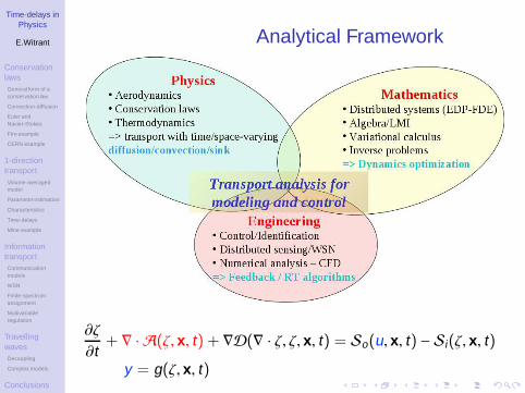
Analytical Framework

∂ζ

∂t+ ∇ · A(ζ, x, t) + ∇D(∇ · ζ, ζ, x, t) = So(u, x, t) − Si(ζ, x, t)

y = g(ζ, x, t)


E.Witrant




Firn example

CERN example



Characteristics

Time-delays

Mine example


WSN




Complex models

Conclusions

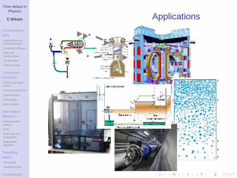
Applications


E.Witrant




Firn example

CERN example



Characteristics

Time-delays

Mine example


WSN




Complex models

Conclusions

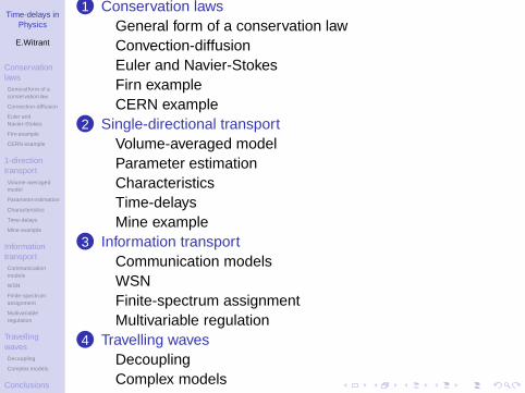
1 Conservation lawsGeneral form of a conservation lawConvection-diffusionEuler and Navier-StokesFirn exampleCERN example

2 Single-directional transportVolume-averaged modelParameter estimationCharacteristicsTime-delaysMine example

3 Information transportCommunication modelsWSNFinite-spectrum assignmentMultivariable regulation

4 Travelling wavesDecouplingComplex models


E.Witrant




Firn example

CERN example



Characteristics

Time-delays

Mine example


WSN




Complex models

Conclusions

Conservation laws

• Model from physics: subatomic, atomics or molecular,microscopic, macroscopic, astronomical scale

• I.e. fluid dynamics = study of the interactive motion andbehavior of a large number of elements

• System of interacting elements as a continuum

• Consider an elementary volume that contains a sufficientlylarge number of molecules with well defined mean velocityand mean kinetic energy

• At each point we can thus infer, e.g. velocity, temperature,pressure, entropy etc.


E.Witrant




Firn example

CERN example



Characteristics

Time-delays

Mine example


WSN




Complex models

Conclusions

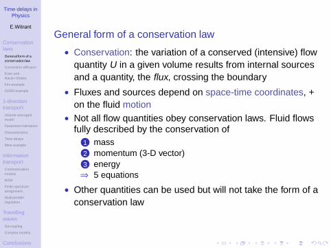
General form of a conservation law

• Conservation: the variation of a conserved (intensive) flowquantity U in a given volume results from internal sourcesand a quantity, the flux, crossing the boundary

• Fluxes and sources depend on space-time coordinates, +on the fluid motion

• Not all flow quantities obey conservation laws. Fluid flowsfully described by the conservation of

1 mass2 momentum (3-D vector)3 energy⇒ 5 equations

• Other quantities can be used but will not take the form of aconservation law


E.Witrant




Firn example

CERN example



Characteristics

Time-delays

Mine example


WSN




Complex models

Conclusions

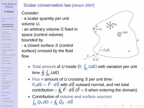
Scalar conservation law [Hirsch 2007]

Consider:- a scalar quantity per unitvolume U,- an arbitrary volume Ω fixed inspace (control volume)bounded by- a closed surface S (controlsurface) crossed by the fluidflow

• Total amount of U inside Ω:∫

ΩUdΩ with variation per unit

time ∂∂t

∫

ΩUdΩ

• Flux = amount of U crossing S per unit time:FndS = ~F · d~S with d~S outward normal, and net totalcontribution −

∮

S~F · d~S (~F > 0 when entering the domain)

• Contribution of volume and surface sources:∫

ΩQV dΩ+

∮

S~QS · d~S


E.Witrant




Firn example

CERN example



Characteristics

Time-delays

Mine example


WSN




Complex models

Conclusions

Scalar conservation law (2)Provides the integral conservation form for quantity U:

∂

∂t

∫

ΩU dΩ+

∮

S

~F · d~S =

∫

ΩQV dΩ+

∮

S

~QS · d~S

• valid ∀ fixed S and Ω, at any point in the flow domain

• internal variation of U depends only of fluxes through S ,not inside

• no derivative/gradient of F : may be discontinuous andadmit shock waves

⇒ relate to conservative numerical scheme at the discretelevel (e.g. conserve mass)


E.Witrant




Firn example

CERN example



Characteristics

Time-delays

Mine example


WSN




Complex models

Conclusions

Differential form of a conservation lawObtained using Gauss’ theorem

∮

S~F · d~S =

∫

Ω~∇ · ~F dΩ as:

∂U∂t

+ ~∇ · ~F = QV + ~∇ · ~QS ⇔∂U∂t

+ ~∇ · (~F − ~QS) = QV

• the effective flux (~F − ~QS) appears exclusively in thegradient operator⇒ way to recognize conservation laws

• more restrictive than the integral form as the flux has to bedifferentiable (excludes shocks)

• fluxes and source definition provided by the quantity Uconsidered


E.Witrant




Firn example

CERN example



Characteristics

Time-delays

Mine example


WSN




Complex models

Conclusions

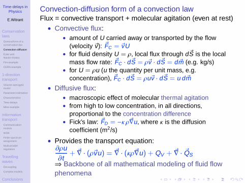
Convection-diffusion form of a convection lawFlux = convective transport + molecular agitation (even at rest)• Convective flux:

• amount of U carried away or transported by the flow(velocity ~v): ~FC = ~vU

• for fluid density U = ρ, local flux through d~S is the localmass flow rate: ~FC · d~S = ρ~v · d~S = d ~m (e.g. kg/s)

• for U = ρu (u the quantity per unit mass, e.g.concentration), ~FC · d~S = ρu~v · d~S = u d ~m

• Diffusive flux:• macroscopic effect of molecular thermal agitation• from high to low concentration, in all directions,

proportional to the concentration difference• Fick’s law: ~FD = −κ ρ~∇u, where κ is the diffusion

coefficient (m2/s)

• Provides the transport equation:∂ρu∂t

+ ~∇ · (ρ~vu) = ~∇ · (κρ~∇u) + QV + ~∇ · ~QS

⇒ Backbone of all mathematical modeling of fluid flowphenomena


E.Witrant




Firn example

CERN example



Characteristics

Time-delays

Mine example


WSN




Complex models

Conclusions

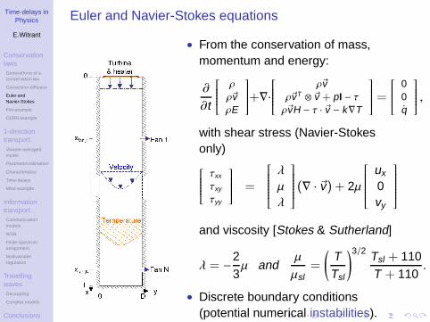
Euler and Navier-Stokes equations

• From the conservation of mass,momentum and energy:

∂

∂t

ρ

ρ~vρE

+∇·

ρ~vρ~vT ⊗ ~v + pI − τρ~vH − τ · ~v − k∇T

=

00q

,

with shear stress (Navier-Stokesonly)

τxx

τxy

τyy

=

λ

µ

λ

(∇ · ~v) + 2µ

ux

0vy

and viscosity [Stokes & Sutherland]

λ = −23µ and

µ

µsl=

(

TTsl

)3/2 Tsl + 110T + 110

.

• Discrete boundary conditions(potential numerical instabilities).


E.Witrant




Firn example

CERN example



Characteristics

Time-delays

Mine example


WSN




Complex models

Conclusions

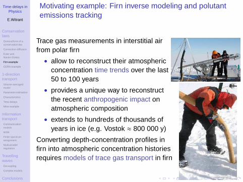
Motivating example: Firn inverse modeling and polutantemissions tracking

Trace gas measurements in interstitial airfrom polar firn

• allow to reconstruct their atmosphericconcentration time trends over the last50 to 100 years

• provides a unique way to reconstructthe recent anthropogenic impact onatmospheric composition

• extends to hundreds of thousands ofyears in ice (e.g. Vostok ≈ 800 000 y)

Converting depth-concentration profiles infirn into atmospheric concentration historiesrequires models of trace gas transport in firn


E.Witrant




Firn example

CERN example



Characteristics

Time-delays

Mine example


WSN




Complex models

Conclusions

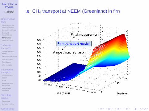
I.e. CH4 transport at NEEM (Greenland) in firn


E.Witrant




Firn example

CERN example



Characteristics

Time-delays

Mine example


WSN




Complex models

Conclusions

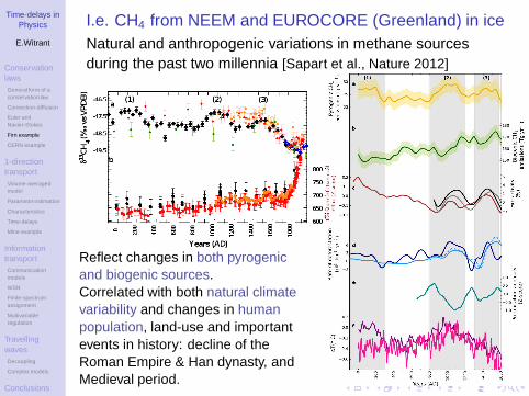
I.e. CH4 from NEEM and EUROCORE (Greenland) in iceNatural and anthropogenic variations in methane sourcesduring the past two millennia [Sapart et al., Nature 2012]

Reflect changes in both pyrogenicand biogenic sources.Correlated with both natural climatevariability and changes in humanpopulation, land-use and importantevents in history: decline of theRoman Empire & Han dynasty, andMedieval period.


E.Witrant




Firn example

CERN example



Characteristics

Time-delays

Mine example


WSN




Complex models

Conclusions

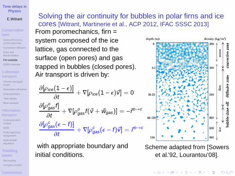
Solving the air continuity for bubbles in polar firns and icecores [Witrant, Martinerie et al., ACP 2012, IFAC SSSC 2013]

From poromechanics, firn =system composed of the icelattice, gas connected to thesurface (open pores) and gastrapped in bubbles (closed pores).Air transport is driven by:

∂[ρice(1 − ǫ)]∂t

+ ∇[ρice(1 − ǫ)~v ] = 0

∂[ρogasf ]

∂t+ ∇[ρo

gas f(~v + ~wgas)] = −~ro→c

∂[ρcgas(ǫ − f)]

∂t+ ∇[ρc

gas(ǫ − f)~v] = ~ro→c

with appropriate boundary andinitial conditions.

Scheme adapted from [Sowerset al.’92, Lourantou’08].


E.Witrant




Firn example

CERN example



Characteristics

Time-delays

Mine example


WSN




Complex models

Conclusions

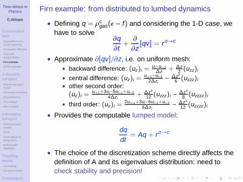
Firn example: from distributed to lumbed dynamics

• Defining q = ρcgas(ǫ − f) and considering the 1-D case, we

have to solve∂q∂t

+∂

∂z[qv] = ro→c

• Approximate ∂[qv]/∂z, i.e. on uniform mesh:• backward difference: (uz)i =

ui−ui−1∆z + ∆z

2 (uzz)i

• central difference: (uz)i =ui+1−ui−1

2∆zi− ∆z2

6 (uzzz)i

• other second order:(uz)i =

ui+1+3ui−5ui−1+ui−2

4∆zi+ ∆z2

12 (uzzz)i − ∆z3

8 (uzzzz)i

• third order: (uz)i =2ui+1+3ui−6ui−1+ui−2

6∆zi− ∆z3

12 (uzzzz)i

• Provides the computable lumped model:

dqdt

= Aq + ro→c

• The choice of the discretization scheme directly affects thedefinition of A and its eigenvalues distribution: need tocheck stability and precision!


E.Witrant




Firn example

CERN example



Characteristics

Time-delays

Mine example


WSN




Complex models

Conclusions

e.g. eig(A) for CH4 at NEEM with dt = 1 month

−2 −1.5 −1 −0.5 0 0.5 1 1.5 2−3

−2

−1

0

1

2

3

Real part of eigenvalues

Imag

inar

y pa

rt o

f eig

enva

lues

0 20 40 60 80 100 120 140 160 180−3

−2.5

−2

−1.5

−1

−0.5

0

0.5

Depth (m)

Rea

l par

t of e

igen

valu

es

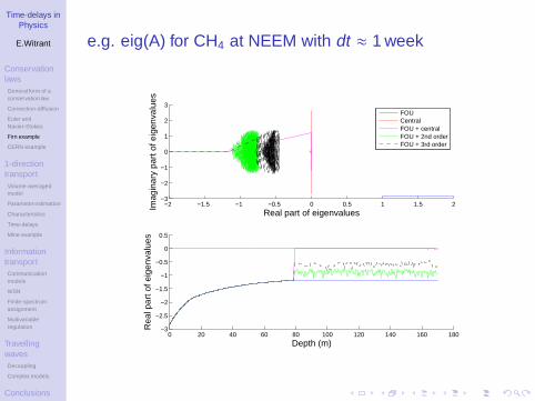
FOUCentralFOU + centralFOU + 2nd orderFOU + 3rd order


E.Witrant




Firn example

CERN example



Characteristics

Time-delays

Mine example


WSN




Complex models

Conclusions

e.g. eig(A) for CH4 at NEEM with dt ≈ 1 week

−2 −1.5 −1 −0.5 0 0.5 1 1.5 2−3

−2

−1

0

1

2

3


Imag

inar

y pa

rt o

f eig

enva

lues

0 20 40 60 80 100 120 140 160 180−3

−2.5

−2

−1.5

−1

−0.5

0

0.5

Depth (m)

Rea

l par

t of e

igen

valu

es



E.Witrant




Firn example

CERN example



Characteristics

Time-delays

Mine example


WSN




Complex models

Conclusions

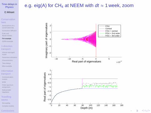
e.g. eig(A) for CH4 at NEEM with dt ≈ 1 week, zoom

−15 −10 −5 0 5

x 10−3

−2

−1

0

1

2


Imag

inar

y pa

rt o

f eig

enva

lues

0 20 40 60 80 100 120 140 160 180−3

−2.5

−2

−1.5

−1

−0.5

0

0.5

1

Depth (m)

Rea

l par

t of e

igen

valu

es



E.Witrant




Firn example

CERN example



Characteristics

Time-delays

Mine example


WSN




Complex models

Conclusions

e.g. Impulse response (Green’s function) for CH4 atNEEM with dt = 1 month

0 20 40 60 80 100 120 140 160 1800.994

0.995

0.996

0.997

0.998

0.999

1

1.001

Depth (m)

Nor

m o

f Gre

en fc

t

0 20 40 60 80 100 120 140 160 1800

5

10

15

20

25

Depth (m)

σ of

Gre

en fc

t



E.Witrant




Firn example

CERN example



Characteristics

Time-delays

Mine example


WSN




Complex models

Conclusions

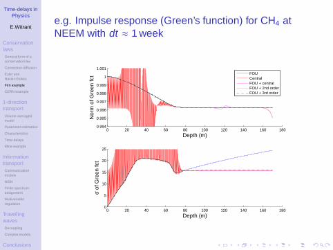
e.g. Impulse response (Green’s function) for CH4 atNEEM with dt ≈ 1 week

0 20 40 60 80 100 120 140 160 1800.994

0.995

0.996

0.997

0.998

0.999

1

1.001

Depth (m)

Nor

m o

f Gre

en fc

t

0 20 40 60 80 100 120 140 160 1800

5

10

15

20

25

Depth (m)

σ of

Gre

en fc

t



E.Witrant




Firn example

CERN example



Characteristics

Time-delays

Mine example


WSN




Complex models

Conclusions

Conclusions on the firn example

• Solution obtained from classical CFD (computational fluiddynamics) analysis

• Purely advective below the bubbles closure→ physically,we want to reflect pure information transport, i.e. delay

• Dynamics represented as an I/O map with the Greenfunction

• The high precision + large sampling time objective isdifficult to meet with a direct numerical approach

• Need to extend the result to variable advection speed

⇒ An analytical approach using time-delays (kernel) for theI/O map could solve the problem


E.Witrant




Firn example

CERN example



Characteristics

Time-delays

Mine example


WSN




Complex models

Conclusions

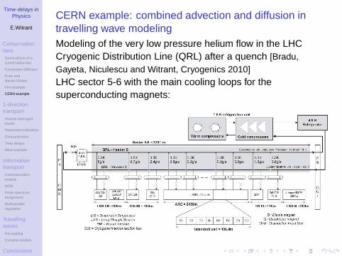
CERN example: combined advection and diffusion intravelling wave modelingModeling of the very low pressure helium flow in the LHCCryogenic Distribution Line (QRL) after a quench [Bradu,Gayeta, Niculescu and Witrant, Cryogenics 2010]LHC sector 5-6 with the main cooling loops for thesuperconducting magnets:


E.Witrant




Firn example

CERN example



Characteristics

Time-delays

Mine example


WSN




Complex models

Conclusions

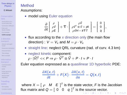
MethodAssumptions:

• model using Euler equation

∂

∂t

ρ

ρ~vρE

+ ∇ ·

ρ~vρ~vT ⊗ ~v + pIρ~vH − k∇T

=

00q

,

• flux according to the x direction only (the main flowdirection) : V = Vx and M = ρ · Vx

• straight line: neglect QRL curvature (rad. of curv. 4.3 km)

• neglect kinetic component:ρ · |~V |2 << P ⇒ ρ · ~VT ⊗ ~V + P · I ≈ P · I

Euler equation expressed as a quasilinear 1D hyperbolic PDE:

∂X(x , t)

∂t+ F(X) · ∂X(x , t)

∂x= Q(x , t)

where X = [ ρ M E ]T is the state vector, F is the Jacobianflux matrix and Q = [ 0 0 q ]T is the source vector.


E.Witrant




Firn example

CERN example



Characteristics

Time-delays

Mine example


WSN




Complex models

Conclusions

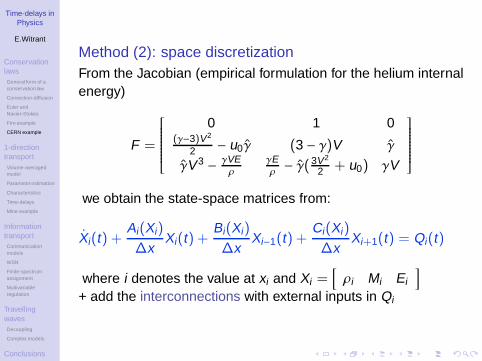
Method (2): space discretizationFrom the Jacobian (empirical formulation for the helium internalenergy)

F =

0 1 0(γ−3)V2

2 − u0γ (3 − γ)V γ

γV3 − γVEρ

γEρ − γ(

3V2

2 + u0) γV

we obtain the state-space matrices from:

Xi(t) +Ai(Xi)

∆xXi(t) +

Bi(Xi)

∆xXi−1(t) +

Ci(Xi)

∆xXi+1(t) = Qi(t)

where i denotes the value at xi and Xi =[

ρi Mi Ei

]

+ add the interconnections with external inputs in Qi


E.Witrant




Firn example

CERN example



Characteristics

Time-delays

Mine example


WSN




Complex models

Conclusions

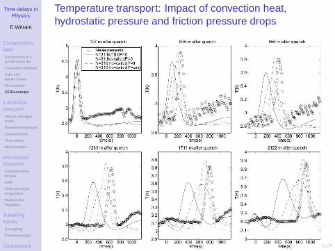
Temperature transport: Impact of convection heat,hydrostatic pressure and friction pressure drops


E.Witrant




Firn example

CERN example



Characteristics

Time-delays

Mine example


WSN




Complex models

Conclusions

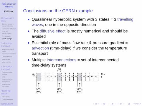
Conclusions on the CERN example

• Quasilinear hyperbolic system with 3 states = 3 travellingwaves, one in the opposite direction

• The diffusive effect is mostly numerical and should beavoided

• Essential role of mass flow rate & pressure gradient =advection (time-delay) if we consider the temperaturetransport

• Multiple interconnections = set of interconnectedtime-delay systems


E.Witrant




Firn example

CERN example



Characteristics

Time-delays

Mine example


WSN




Complex models

Conclusions

Single-directional transport

Suppose that we want to control a unidirectional, mostlyadvective, process through the boundary: can a time-delayapproach help?Proposed strategy:

1 starting from Euler’s equation, isolate the variable ofinterest

2 simplify the model to define an observer/estimationstructure

3 use the estimated parameter for a lumped control-orientedmodel with transport as a delay

4 choose a stabilizing feedback


E.Witrant




Firn example

CERN example



Characteristics

Time-delays

Mine example


WSN




Complex models

Conclusions

Volume-averaged model for pressure regulation

• From energy conservation in Euler & phys. hypoteses:

∂p∂t

= − ∂∂x

[

Mρ·(

1 +Rcv

)

p

]

+Rcv

q

• Volume-averaged impact of momentum and density:X(t) 1

V∮

V X(v , t)dv, for X M, ρ• Energy losses = pressure losses (friction and exhausts),

e.g. q(x , t)R/cv = s(x , t) + r(t)p(x , t)

• Leads to the PDE model with boundary (controlled) input:

pt = c(t)px + r(t)p + s(x , t),p(0, t) = pin(t), p(x , 0) = p0(x)

⇒ Given distributed measurements, estimate transportcoefficients and set feedback pin(t)


E.Witrant




Firn example

CERN example



Characteristics

Time-delays

Mine example


WSN




Complex models

Conclusions

Observer-based online parameter estimation [W,Marchand’08]

Theorem (parameter estimation for affine PDE) :Consider the class of systems, affine in the parameter

pt = A(p, px , pxx , u, ϑ)ϑa1px(0, t) + a2p(0, t) = a3

a4px(L , t) + a5p(L , t) = a6

with distributed measurements of p(x , t) and for which wewant to estimate ϑ. Then

||p(x, t) − p(x, t)||22 = e−2(γ+λ)t ||p(x, 0) − p(x, 0)||22

if

pt = A(p, px , pxx , u, ϑ)ϑ+ γ(p − p)a1px(0, t) + a2p(0, t) = a3

a4px(L , t) + a5p(L , t) = a6

ϑ = A(p, px , pxx , u, ϑ)†[pt + λ(p − p)]


E.Witrant




Firn example

CERN example



Characteristics

Time-delays

Mine example


WSN




Complex models

Conclusions

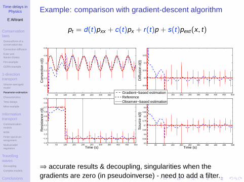
Example: comparison with gradient-descent algorithm

pt = d(t)pxx + c(t)px + r(t)p + s(t)pext(x , t)

0 50 100 150 200 250 300 350 400 450 500

−1.3

−1.2

−1.1

−1

−0.9

−0.8

Con

vect

ion

c(t)

0 50 100 150 200 250 300 350 400 450 5000.4

0.45

0.5

0.55

0.6

0.65

Diff

usio

n d(

t)

0 50 100 150 200 250 300 350 400 450 500−1.5

−1.4

−1.3

−1.2

−1.1

−1

−0.9

−0.8

−0.7

−0.6

−0.5

Res

ista

nce

r(t)

Time (s)0 50 100 150 200 250 300 350 400 450 500

0.5

0.55

0.6

0.65

0.7

0.75

0.8

0.85

0.9

0.95

1

Sou

rce

s(t)

Time (s)

Gradient−based estimationReferenceObserver−based estimation

⇒ accurate results & decoupling, singularities when thegradients are zero (in pseudoinverse) - need to add a filter.


E.Witrant




Firn example

CERN example



Characteristics

Time-delays

Mine example


WSN




Complex models

Conclusions

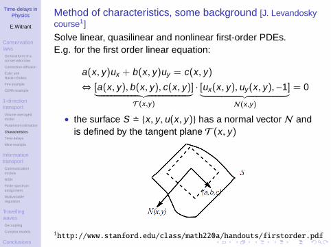
Method of characteristics, some background [J. Levandoskycourse1]

Solve linear, quasilinear and nonlinear first-order PDEs.E.g. for the first order linear equation:

a(x , y)ux + b(x , y)uy = c(x , y)

⇔ [a(x , y), b(x , y), c(x , y)]︸︷︷︸

T (x ,y)

· [ux(x , y), uy(x , y),−1]︸︷︷︸

N(x ,y)

= 0

• the surface S x , y , u(x , y) has a normal vector N andis defined by the tangent plane T (x , y)

1http://www.stanford.edu/class/math220a/handouts/firstorder.pdf

http://www.stanford.edu/class/math220a/handouts/firstorder.pdf


E.Witrant




Firn example

CERN example



Characteristics

Time-delays

Mine example


WSN




Complex models

Conclusions

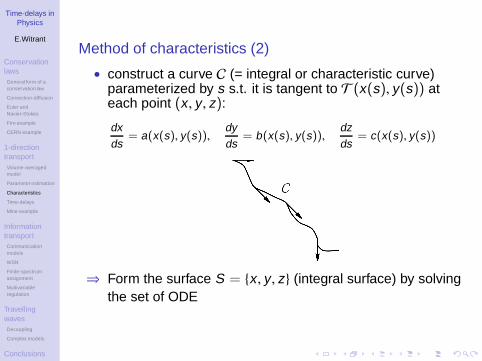
Method of characteristics (2)

• construct a curve C (= integral or characteristic curve)parameterized by s s.t. it is tangent to T (x(s), y(s)) ateach point (x , y , z):

dxds

= a(x(s), y(s)),dyds

= b(x(s), y(s)),dzds

= c(x(s), y(s))

⇒ Form the surface S = x , y , z (integral surface) by solvingthe set of ODE


E.Witrant




Firn example

CERN example



Characteristics

Time-delays

Mine example


WSN




Complex models

Conclusions

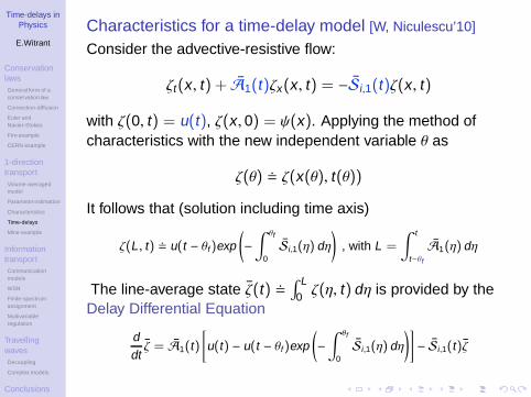
Characteristics for a time-delay model [W, Niculescu’10]

Consider the advective-resistive flow:

ζt(x , t) + A1(t)ζx(x , t) = −Si,1(t)ζ(x , t)

with ζ(0, t) = u(t), ζ(x , 0) = ψ(x). Applying the method ofcharacteristics with the new independent variable θ as

ζ(θ) ζ(x(θ), t(θ))

It follows that (solution including time axis)

ζ(L , t) u(t − θf)exp

(

−∫ θf

0Si,1(η) dη

)

, with L =

∫ t

t−θf

A1(η) dη

The line-average state ζ(t) ∫ L0ζ(η, t) dη is provided by the

Delay Differential Equation

ddtζ = A1(t)

[

u(t) − u(t − θf)exp

(

−∫ θf

0Si,1(η) dη

)]

− Si,1(t)ζ


E.Witrant




Firn example

CERN example



Characteristics

Time-delays

Mine example


WSN




Complex models

Conclusions

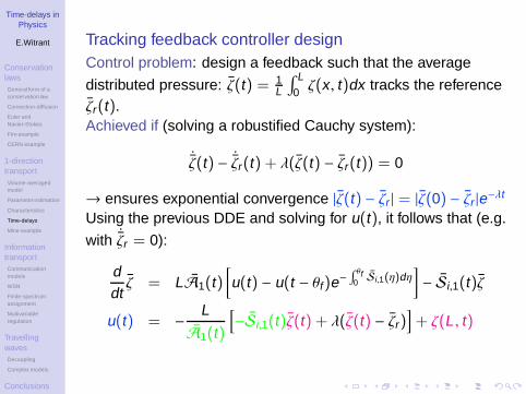
Tracking feedback controller designControl problem: design a feedback such that the average

distributed pressure: ζ(t) = 1L

∫ L0ζ(x , t)dx tracks the reference

ζr(t).Achieved if (solving a robustified Cauchy system):

˙ζ(t) − ˙ζr(t) + λ(ζ(t) − ζr(t)) = 0

→ ensures exponential convergence |ζ(t) − ζr | = |ζ(0) − ζr |e−λt

Using the previous DDE and solving for u(t), it follows that (e.g.

with ˙ζr = 0):

ddtζ = LA1(t)

[

u(t) − u(t − θf)e−

∫ θf0Si,1(η)dη

]

− Si,1(t)ζ

u(t) = − L

A1(t)

[

−Si,1(t)ζ(t) + λ(ζ(t) − ζr)]

+ ζ(L , t)


E.Witrant




Firn example

CERN example



Characteristics

Time-delays

Mine example


WSN




Complex models

Conclusions

Mining ventilation example: reference model

Simulator properties:

• ventilation shafts ≈ 28 control volumes(CV), 3 extraction levels

• regulation of the turbine and fans

• flows, pressures and temperaturesmeasured in each CV

• Computation 34× faster than real-time

Case study:

• 1st level fan not used (natural airflow), 2nd

operated at 1000 s (150 rpm) and 3rd runscontinuously (200 rpm)

• CO pollution injected in 3rd level

• measurement of flow speed, pressure,temperature and pollution at the surfaceand extraction levels


E.Witrant




Firn example

CERN example



Characteristics

Time-delays

Mine example


WSN




Complex models

Conclusions

Feedback control results for mine ventilation

Reference and effective turbine output pressure:

0 200 400 600 800 1000 1200 1400 1600 1800 20001.03

1.04

1.05

1.06

1.07

1.08

1.09

1.1

1.11

1.12

1.13

1.14x 10

5

Time (s)

Turb

ine

pre

ssure

(Pa)

Effective

Reference

Feedback tracking error:

0 200 400 600 800 1000 1200 1400 1600 1800 200010

−4

10−2

100

102

104

Time (s)

Tra

ckin

ger

ror

(Pa)

⇒ Sensible to initial conditions and some numerical integrationerrors but exponential convergence verified!


E.Witrant




Firn example

CERN example



Characteristics

Time-delays

Mine example


WSN




Complex models

Conclusions

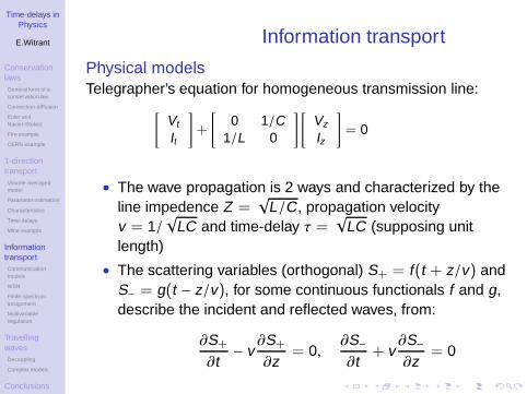
Information transport

Physical modelsTelegrapher’s equation for homogeneous transmission line:

[

Vt

It

]

+

[

0 1/C1/L 0

] [

Vz

Iz

]

= 0

• The wave propagation is 2 ways and characterized by theline impedence Z =

√L/C, propagation velocity

v = 1/√

LC and time-delay τ =√

LC (supposing unitlength)

• The scattering variables (orthogonal) S+ = f(t + z/v) andS− = g(t − z/v), for some continuous functionals f and g,describe the incident and reflected waves, from:

∂S+

∂t− v

∂S+

∂z= 0,

∂S−∂t

+ v∂S−∂z

= 0


E.Witrant




Firn example

CERN example



Characteristics

Time-delays

Mine example


WSN




Complex models

Conclusions

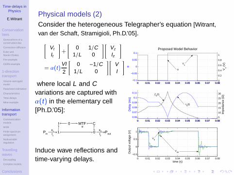
Physical models (2)Consider the heterogeneous Telegrapher’s equation [Witrant,van der Schaft, Stramigioli, Ph.D.’05].

[

Vt

It

]

+

[

0 1/C1/L 0

] [

Vz

Iz

]

= α(t)VI2

[

0 −1/C1/L 0

] [

VI

]

where local L and Cvariations are captured withα(t) in the elementary cell[Ph.D.’05]:

e1

f1

e2

f2

I C

1 0Pin Pout

MTF0 . .α

Induce wave reflections andtime-varying delays.

0 0.01 0.02 0.03 0.04 0.05 0.06 0.07 0.08−0.1

−0.05

0

0.05

0.1

α

0 0.01 0.02 0.03 0.04 0.05 0.06 0.07 0.080

0.2

0.4

0.6

0.8

1

Vs (

V)

Proposed Model Behavior

0 0.01 0.02 0.03 0.04 0.05 0.06 0.07 0.08

0.06

0.07

0.08

0.09

0.1

0.11

Del

ay (

ms)

0 0.01 0.02 0.03 0.04 0.05 0.06 0.07 0.085

10

15

20

25

30

Impe

danc

e (Ω

)

0 0.01 0.02 0.03 0.04 0.05 0.06 0.07 0.08

−0.5

0

0.5

1O

utpu

t vol

tage

(V

)

time (s)

Vh

Vnh

τ5(t)

Z5(t)

Vs

α


E.Witrant




Firn example

CERN example



Characteristics

Time-delays

Mine example


WSN




Complex models

Conclusions

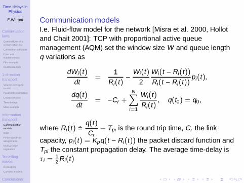
Communication modelsI.e. Fluid-flow model for the network [Misra et al. 2000, Hollotand Chait 2001]: TCP with proportional active queuemanagement (AQM) set the window size W and queue lengthq variations as

dWi(t)

dt=

1Ri(t)

− Wi(t)

2

Wi(t − Ri(t))

Ri(t − Ri(t))pi(t),

dq(t)

dt= −Cr +

N∑

i=1

Wi(t)

Ri(t), q(t0) = q0,

where Ri(t) q(t)Cr

+ Tpi is the round trip time, Cr the link

capacity, pi(t) = Kpq(t − Ri(t)) the packet discard function andTpi the constant propagation delay. The average time-delay isτi =

12Ri(t)


E.Witrant




Firn example

CERN example



Characteristics

Time-delays

Mine example


WSN




Complex models

Conclusions

Wireless Sensor Networks[Park, di Marco, Soldati, Fischione, Johansson’09...]

PAN coordinator

Sensor

• IEEE 802.15.4, Markov chain model, network & controlcodesign

• Communication constraints = time-delay + packet loss


E.Witrant




Firn example

CERN example



Characteristics

Time-delays

Mine example


WSN




Complex models

Conclusions

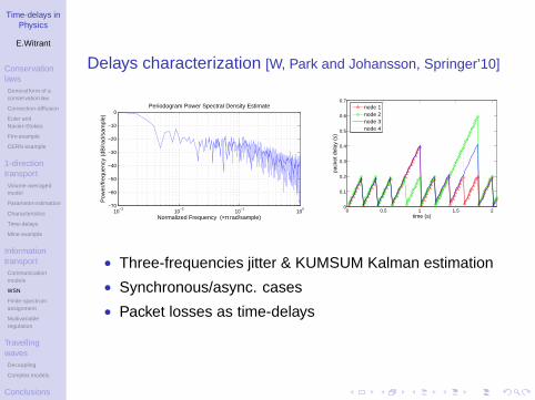
Delays characterization [W, Park and Johansson, Springer’10]

10−3

10−2

10−1

100

−70

−60

−50

−40

−30

−20

−10

0

Normalized Frequency (×π rad/sample)

Pow

er/fr

eque

ncy

(dB

/rad

/sam

ple)

Periodogram Power Spectral Density Estimate

0 0.5 1 1.5 20

0.1

0.2

0.3

0.4

0.5

0.6

0.7

time (s)

pack

et d

elay

(s)

node 1node 2node 3node 4

• Three-frequencies jitter & KUMSUM Kalman estimation

• Synchronous/async. cases

• Packet losses as time-delays


E.Witrant




Firn example

CERN example



Characteristics

Time-delays

Mine example


WSN




Complex models

Conclusions

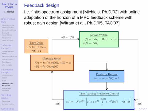
Feedback designI.e. finite-spectrum assignment [Michiels, Ph.D.’02] with onlineadaptation of the horizon of a MPC feedback scheme withrobust gain design [Witrant et al., Ph.D.’05, TAC’07]

z(t) = f(z(t), ud(t)), z(0) = z0

τ(t) = h(z(t), ud(t))

x(t) = Ax(t) + Bu(t − τ(t))

y(t) = Cx(t)

Linear System

Network Model

δ(t) − τ(t + δ(t)) = 0

Predictor Horizon

u(t) = −KeAδ(t)

[

x(t) + eAt

t+δ(t)∫

t

e−AθBu(θ − τ(θ))dθ

]

Time-Varying Predictive Control

0 ≤ τ(t) ≤ τmax

τ (t) < 1

Time-Delay

u(t)

u(t − τ(t))

x(t)


E.Witrant




Firn example

CERN example



Characteristics

Time-delays

Mine example


WSN




Complex models

Conclusions

Example: control of an inverted pendulum over a network


E.Witrant




Firn example

CERN example



Characteristics

Time-delays

Mine example


WSN




Complex models

Conclusions

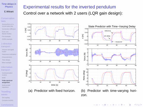
Experimental results for the inverted pendulumControl over a network with 2 users (LQR gain design):

0 10 20 30 40 50−0.02

−0.01

0

0.01

0.02

0.03x

(m)

0 10 20 30 40 50−10

−5

0

5

10

forc

e (N

)

0 10 20 30 40 50−20

−10

0

10

20

θ (d

eg)

time (s)

(a) Predictor with fixed horizon.

0 10 20 30 40 50−0.02

−0.01

0

0.01

0.02State Predictor with Time−Varying Delay

x (m

)

0 10 20 30 40 50−2

−1

0

1

2

forc

e (N

)0 10 20 30 40 50

−10

−5

0

5

10

15

thet

a (d

eg)

reference

measured

w/o delay

(b) Predictor with time-varying hori-zon.


E.Witrant




Firn example

CERN example



Characteristics

Time-delays

Mine example


WSN




Complex models

Conclusions

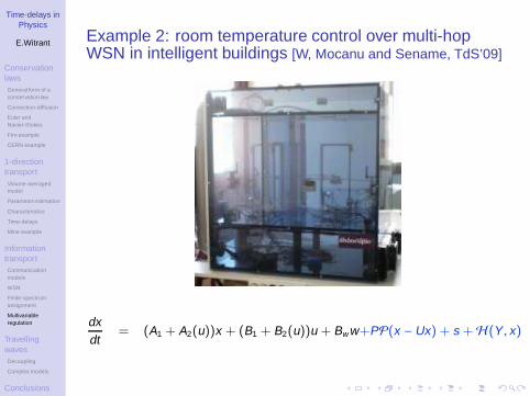
Example 2: room temperature control over multi-hopWSN in intelligent buildings [W, Mocanu and Sename, TdS’09]

dxdt

= (A1 + A2(u))x + (B1 + B2(u))u + Bww+PP(x − Ux) + s +H(Y , x)


E.Witrant




Firn example

CERN example



Characteristics

Time-delays

Mine example


WSN




Complex models

Conclusions

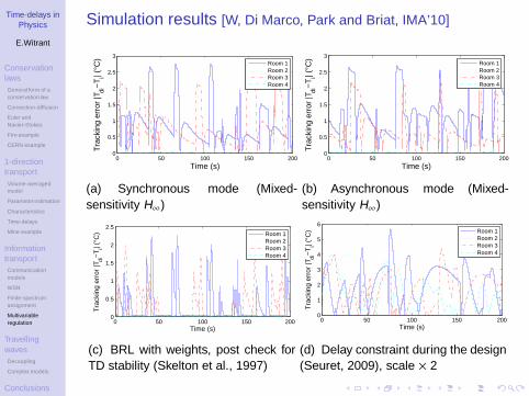
Simulation results [W, Di Marco, Park and Briat, IMA’10]

0 50 100 150 2000

0.5

1

1.5

2

2.5

3

Tra

ckin

g er

ror

|Tdi

−T

i| (°C

)

Time (s)

Room 1Room 2Room 3Room 4

(a) Synchronous mode (Mixed-sensitivity H∞)

0 50 100 150 2000

0.5

1

1.5

2

2.5

3

Tra

ckin

g er

ror

|Tdi

−T

i| (°C

)

Time (s)


(b) Asynchronous mode (Mixed-sensitivity H∞)

0 50 100 150 2000

0.5

1

1.5

2

2.5

Tra

ckin

g er

ror

|Tdi

−T

i| (°C

)

Time (s)


(c) BRL with weights, post check forTD stability (Skelton et al., 1997)

0 50 100 150 2000

1

2

3

4

5

6

Tra

ckin

g er

ror

|Tdi

−T

i| (°C

)

Time (s)


(d) Delay constraint during the design(Seuret, 2009), scale × 2


E.Witrant




Firn example

CERN example



Characteristics

Time-delays

Mine example


WSN




Complex models

Conclusions

Conclusions on 1-direction and information transport

• Direct equivalence between time-delays and advectivetransport for single-directional transport and homogenous(possibly time-varying) coefficients

• Equivalence obtained for two waves in homogeneoustransmission lines from the scattering variables

• Time-delay with router feedback in communicationnetworks

• Possible online addaptation of the controller’s sizeaccording to the delay variations with the predictorarchitecture

• Strong impact of signal distorsion in WSN may call forrobustness rather than time-delay compensation


E.Witrant




Firn example

CERN example



Characteristics

Time-delays

Mine example


WSN




Complex models

Conclusions

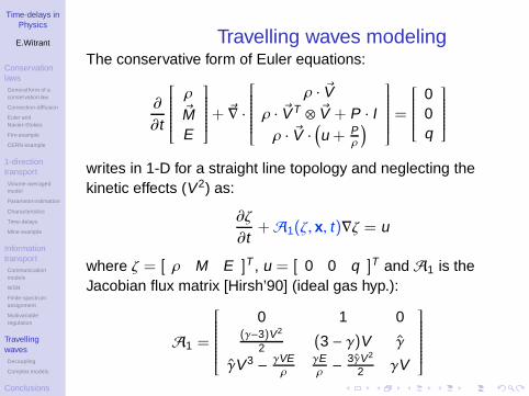
Travelling waves modelingThe conservative form of Euler equations:

∂

∂t

ρ~ME

+ ~∇ ·

ρ · ~Vρ · ~VT ⊗ ~V + P · Iρ · ~V ·

(

u + Pρ

)

=

00q

writes in 1-D for a straight line topology and neglecting thekinetic effects (V2) as:

∂ζ

∂t+A1(ζ, x, t)∇ζ = u

where ζ = [ ρ M E ]T , u = [ 0 0 q ]T and A1 is theJacobian flux matrix [Hirsh’90] (ideal gas hyp.):

A1 =

0 1 0(γ−3)V2

2 (3 − γ)V γ

γV3 − γVEρ

γEρ −

3γV2

2 γV


E.Witrant




Firn example

CERN example



Characteristics

Time-delays

Mine example


WSN




Complex models

Conclusions

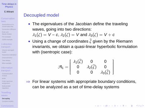
Decoupled model

• The eigenvalues of the Jacobian define the travelingwaves, going into two directions:λ1(ζ) = V − c, λ2(ζ) = V and λ3(ζ) = V + c

• Using a change of coordinates ζ given by the Riemanninvariants, we obtain a quasi-linear hyperbolic formulationwith (isentropic case):

A1 =

λ1(ζ) 0 00 λ2(ζ) 00 0 λ3(ζ)

⇒ For linear systems with appropriate boundary conditions,can be analyzed as a set of time-delay systems


E.Witrant




Firn example

CERN example



Characteristics

Time-delays

Mine example


WSN




Complex models

Conclusions

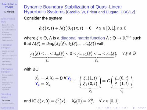
Dynamic Boundary Stabilization of Quasi-LinearHyperbolic Systems [Castillo, W, Prieur and Dugard, CDC’12]

Consider the system

∂tξ(x , t) + Λ(ξ)∂xξ(x , t) = 0 ∀ x ∈ [0, 1], t ≥ 0

where ξ ∈ Θ, Λ is a diagonal matrix function Λ : Θ→ Rn×n suchthat Λ(ξ) = diag(λ1(ξ), λ2(ξ), ..., λn(ξ)) with

λ1(ξ) < ... < λm(ξ)︸︷︷︸

ξ−

< 0 < λm+1(ξ) < ... < λn(ξ)︸︷︷︸

ξ+

, ∀ ξ ∈ Θ

with BC

Xc = A Xc + B KYξ

Yc = Xc;

(

ξ−(1, t)ξ+(0, t)

)

︸︷︷︸

Yc

= G

(

ξ−(0, t)ξ+(1, t)

)

︸︷︷︸

Yξ

and IC ξ(x , 0) = ξ0(x), Xc(0) = X0c , ∀ x ∈ [0, 1].


E.Witrant




Firn example

CERN example



Characteristics

Time-delays

Mine example


WSN




Complex models

Conclusions

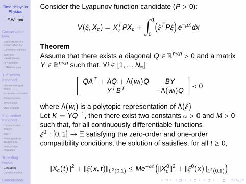
Consider the Lyapunov function candidate (P > 0):

V(ξ,Xc) = XTc PXc +

∫ 1

0

(

ξTPξ)

e−µxdx

TheoremAssume that there exists a diagonal Q ∈ Rn×n > 0 and a matrixY ∈ Rn×n such that, ∀i ∈ [1, ...,Nϕ]

[

QAT + AQ + Λ(wi)Q BYYT BT −Λ(wi)Q

]

≺ 0

where Λ(wi) is a polytopic representation of Λ(ξ)Let K = YQ−1, then there exist two constants α > 0 and M > 0such that, for all continuously differentiable functionsξ0 : [0, 1]→ Ξ satisfying the zero-order and one-ordercompatibility conditions, the solution of satisfies, for all t ≥ 0,

||Xc(t)||2 + ||ξ(x , t)||L2(0,1) ≤ Me−αt(

||X0c ||2 + ||ξ0(x)||L2(0,1)

)


E.Witrant




Firn example

CERN example



Characteristics

Time-delays

Mine example


WSN




Complex models

Conclusions

Example on flow dynamics: Video

A change of reference from V = [1.16, 20, 100000]T toV = [1.2, 30, 105000]T is introduced.


E.Witrant




Firn example

CERN example



Characteristics

Time-delays

Mine example


WSN




Complex models

Conclusions

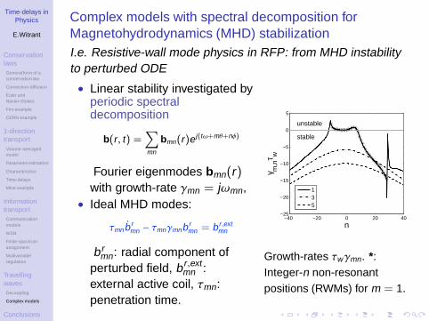
Complex models with spectral decomposition forMagnetohydrodynamics (MHD) stabilizationI.e. Resistive-wall mode physics in RFP: from MHD instabilityto perturbed ODE

• Linear stability investigated byperiodic spectraldecomposition

b(r , t) =∑

mn

bmn(r)ej(tω+mθ+nφ)

Fourier eigenmodes bmn(r)with growth-rate γmn = jωmn,

• Ideal MHD modes:

τmn b rmn − τmnγmnb r

mn = b r ,extmn

b rmn: radial component of

perturbed field, b r ,extmn :

external active coil, τmn:penetration time.

−40 −20 0 20 40−25

−20

−15

−10

−5

0

5

γ m,n

τ w

n

unstable

stable

135

Growth-rates τwγmn. *:Integer-n non-resonantpositions (RWMs) for m = 1.


E.Witrant




Firn example

CERN example



Characteristics

Time-delays

Mine example


WSN




Complex models

Conclusions

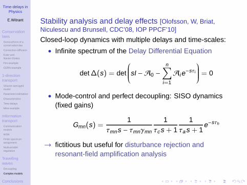
Stability analysis and delay effects [Olofsson, W, Briat,Niculescu and Brunsell, CDC’08, IOP PPCF’10]

Closed-loop dynamics with multiple delays and time-scales:

• Infinite spectrum of the Delay Differential Equation

det∆(s) = det

sI −A0 −n∑

i=1

Aie−sτi

= 0

• Mode-control and perfect decoupling: SISO dynamics(fixed gains)

Gmn(s) =1

τmns − τmnγmn

1τcs + 1

1τas + 1

e−sτh

→ fictitious but useful for disturbance rejection andresonant-field amplification analysis


E.Witrant




Firn example

CERN example



Characteristics

Time-delays

Mine example


WSN




Complex models

Conclusions

Experimental results

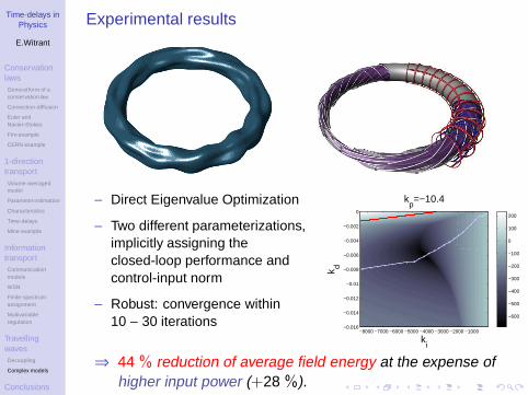
− Direct Eigenvalue Optimization

− Two different parameterizations,implicitly assigning theclosed-loop performance andcontrol-input norm

− Robust: convergence within10 − 30 iterations

ki

k d

kp=−10.4

−8000 −7000 −6000 −5000 −4000 −3000 −2000 −1000−0.016

−0.014

−0.012

−0.01

−0.008

−0.006

−0.004

−0.002

0

−600

−500

−400

−300

−200

−100

0

100

200

⇒ 44 % reduction of average field energy at the expense ofhigher input power (+28 %).


E.Witrant




Firn example

CERN example



Characteristics

Time-delays

Mine example


WSN




Complex models

Conclusions

Conclusions

• Physical delay is often a major issue in transportphenomena; Time-delay systems can often be usefull

• Its proper inclusion in the feedback architecturecompensates advection and losses can be dealt with anintegral action

• Information transport strongly affected by informationlosses and needs robustness

• Capturing the traveling wave requires finer modeling


E.Witrant




Firn example

CERN example



Characteristics

Time-delays

Mine example


WSN




Complex models

Conclusions

Main references• J. Anderson, Fundamentals of Aerodynamics, McGraw-Hill, 1991.

• C. Hirsch, Numerical Computation of Internal & External Flows: theFundamentals of Computational Fluid Dynamics, 2nd ed.Butterworth-Heinemann (Elsevier), 2007.

• E. Witrant, S.I. Niculescu, “Modeling and Control of Large ConvectiveFlows with Time-Delays”, Mathematics in Engineering, Science andAerospace, Vol 1, No 2, 191-205, 2010.http://www.gipsa-lab.grenoble-inp.fr/˜e.witrant/papers/10_Witrant_MESA.pdf

• B. Bradu, P. Gayeta, S.-I. Niculescu and E. Witrant, ”Modeling of thevery low pressure helium ow in the LHC Cryogenic Distribution Lineafter a quench”, Cryogenics, vol. 50 (2), pp. 71-77, Feb. 2010.http://www.gipsa-lab.grenoble-inp.fr/˜e.witrant/papers/09_Simu_QRL.pdf

• E. Olofsson, E. Witrant, C. Briat, S.I. Niculescu and P. Brunsell,”Stability analysis and model-based control in EXTRAP-T2R withtime-delay compensation”, Proc. of 47th IEEE Conference on Decisionand Control, 2008.http://www.gipsa-lab.grenoble-inp.fr/˜e.witrant/papers/08_cdc-olo-6p-rev.pdf

• F. Castillo, E. Witrant, C. Prieur and L. Dugard: Boundary Observers forLinear and Quasi-Linear Hyperbolic Systems with Application to FlowControl, Automatica, to appear, 2013.

http://www.gipsa-lab.grenoble-inp.fr/~e.witrant/papers/10_Witrant_MESA.pdf

http://www.gipsa-lab.grenoble-inp.fr/~e.witrant/papers/09_Simu_QRL.pdf

http://www.gipsa-lab.grenoble-inp.fr/~e.witrant/papers/08_cdc-olo-6p-rev.pdf

Documents

Time-delays in Physics - Gipsa-lab in Physics: From advection to time-delay systems ... Roman Empire & Han dynasty, and Medieval period. Time-delays in Physics