INTERNSHIP REPORT

Time Course study of Gene Expression in Chlamydomonas

reinhardtii during a State 1 to State 2 Transition using Microarray

technology

An internship report presented in partial fulfillment of the requirement of the Professional Science Master's

in Computational Biosciences

Krupa Arun Navalkar

Computational Biosciences Program Arizona State University

Dr. Scott E. Bingham, Ph.D. Internship Advisor

School of Life Sciences Arizona State University

Dr. Jeffrey Touchman, Ph.D.

Dr. Jackiewicz Zdzislaw, Ph.D. Committee Members

Technical Report Number: 07-15

Acknowledgement

This work would not have been possible without the support and guidance of

Dr. Scott Bingham, who has given me the opportunity to work with him on

this project. I am grateful to Dr. Jeffrey Touchman and Dr. Zdzislaw

Jackiewicz for providing me with their invaluable feedback and constant

support. I would like to thank Dr. Rosemary Renaut for her valuable

guidance throughout the program.

I would also like to thank Mr. Jeffery Hock and Ms. Dee Plueard at the DNA

Lab for creating an environment where students can work with and learn

from them. In addition, I would also like to acknowledge Ms. Allison Morse,

Mr. Scott Rusin and Ms. Gowthami Putumbaka for their contributions

towards this project.

Last, but not the least, I would like to thank Mrs. Renate Mittelmann, my

Family and Friends….for always being there.

2

Index

1. Abstract

2. Introduction

3. Discussion

4. Methods and Results

5. Future Work - Recommendations

6. References

7. Appendix

3

List of Figures

Figure 1: General Representation of Dye labeling in a Gene Expression

Microarray (Reece, 2004, Pg. 320 Fig.10.3)………………...…………….……..……...10

Figure 2: Agilent Technologies Microarray Scanner G2565BA ……………….……….14

Figure 3: General Workflow of a Microarray experiment (Draghici, 2003, Pg. 41

Fig.3.6)…...………………………………………………………………………………15

Figure 4: Gel and Electropherogram images of previously purified and

DNase I treated samples………………………………………………………………….23

Figure 5: Venn Diagram of 2 Fold Change lists for all 3 time points (30,60,and 120)

from GeneSpring GX 9.0 Experiment: Chlamy 30,60,120 Corr….……………………..29

Figure 6: Venn Diagram of 2 Fold Change, one way T-test lists for all 3 time points

(30, 60, and 120 minutes) from GeneSpring GX 9.0 Experiment:

Chlamy30,60,120Corr (Venn2)…………………………….……………………………30

Figure 7: Venn Diagram of 2 Fold Change lists for all 3 time points (30, 60 and 120)

from GeneSpring GX 9.0 Experiment: Chlamy 30,60,120+Validate …………………...31

Figure 8: Venn Diagram of 2 Fold Change, 1 way T-test lists for all 3 time points

(30,60,and 120) (Venn2) from GeneSpring GX 9.0 Experiment:

Chlamy30,60,120+Validate…………...............................................................................32

4

List of Tables

Table 1: GeneSpring GX 9.0 Experiment: Chlamy 30,60,120Corr

Summary Data ………………………………………………………………………….30

Table 2: GeneSpring GX 9.0 Experiment: Chlamy30,60,120+Validate

Summary Data…………………………………………………………………………..32

Table 3: Some of the photosystem related genes observed within individual

time point gene lists…………………………………………………………..…………34

Table 4: Some genes of interest from the 160 genes, seen to be commonly

expressed or repressed 2 fold between the three time points………………….………...35

5

Abstract

Chlamydomonas reinhardtii is a photosynthetic, single celled, motile, green alga which

produces energy through the use of light and carbon source. It is commonly seen to grow

in soil, pools and ponds etc. Despite being photosynthetic, they are also known to be able

to grow in the dark. By placing the organism under anoxic stress, without light, its

Photosynthetic State Transition mechanism may be studied.

Chlamydomonas has two photosystems, PS-I (predominantly absorbs far-red light,

700nm) and PS-II (predominantly absorbs red light, 680nm). For optimum utilization of

light energy and electron transport between the two photosystems to continue smoothly,

it is essential to regulate the partitioning of light energy related excitation within the two

photosystems. The Light Harvesting Chlorophylls, LHC-I and LHC-II are the antennae

for PS-I and PS-II respectively. Photoinhibition is the damage occurring to the

photosynthetic apparatus due to excessive absorption of light energy by one photosystem,

leading to energy imbalances within the two interdependent photosystems. State

transition is a mechanism whereby the organism prohibits photoinhibition via the

reversible phosphorylation of LHC-II and migration from PS-II to PS-I.

The aim of the main experiment was to study this shift in photosynthetic apparatus

through gene expression changes caused due to the changes in the organisms’

environmental conditions leading to state transitions. The aim of this project is to outline

the change in expression pattern of certain genes over all three time points (30, 60 and

120 minutes), thereby making them an indicator of the change occurring in genetic

expression due to changing environmental conditions.

At the 30 minute time point, 928 genes were seen to be 2 fold induced or repressed. 2063

genes were seen to be 2 fold up or down regulated in the 60 minute time point and 1652

genes in the 120 minute time point, respectively. A hundred and sixty of these genes are

seen to be either induced or repressed in common within all three time points. These 160

6

genes are the current focus of our study, so as to understand regulation of these genes

across all three time points. This would thus be indicative of changes occurring in the

Photosystems during State Transition. These gene sequences were further put through a

BLAST search so as to associate them with the latest annotation data available for the

same.

A Validation Experiment was also conducted wherein 6 slides, two slides per time point,

were processed in the Normal condition of dye ratio, using old and new RNA preps so as

to eliminate Personnel and Experimental error. The microarray data obtained from these

slides was compared against 9 Normal slides from the Original experiment from all three

time points using GeneSpring and a one way ANOVA t-test was performed in between

these original and validation slides at the 3 specific time points (30, 60 and 120 minutes).

It was found that very few genes were statistically significantly different in these

comparison groups thereby eliminating any experimental or personnel error. Therefore,

we could use the data from even the Validation Experiment as the slides being added into

the original dataset of 18 slides are not very different and would only add to the

replicates.

Future work involves analyzing the 2 fold up or down regulation (induction/ repression)

change lists obtained from this experimental data and developing a model reflecting the

changes occurring within the Photosystems during State Transitions.

7

Introduction

Chlamydomonas reinhardtii is a model organism for many studies related to

photosynthesis. The project data under study involves studying the change in

photosynthesis related gene expression in the organism Chlamydomonas (strain CC-125)

under different growth conditions at three time points using microarray technology. It is

also a model organism for the study of production of Hydrogen as a renewable source of

energy, but this is not the focus of our research. It is a model organism, because despite

being eukaryotic, it is easy to handle through simple microbiological techniques and it is

non-pathogenic. It has a fast mitotic life cycle (generation time=5hrs) and can also

undergo controlled sexual reproduction. The total genome size is approximately 120

Mega bases with 17 haploid chromosomes meaning, it has only a single copy of each

gene making it excellent for studying mutations in-vitro.

Chlamydomonas has two photosystems PS-I (predominantly absorbs far-red light,

700nm) and PS-II (predominantly absorbs red light, 680nm). For optimal utilization of

light energy and electron transport between the two photosystems to continue smoothly,

it is essential to regulate the partitioning of light energy related excitation within the two

photosystems. The Light Harvesting Chlorophylls, LHC-I and LHC-II are the antennae

for PS-I and PS-II respectively. Photoinhibition is the damage occurring to the

photosynthetic apparatus due to excessive absorption of light energy by one photosystem,

leading to energy imbalances within the two interdependent photosytems. A State

transition is a mechanism whereby the organism prohibits photoinhibition via the

reversible phosphorylation of LHC-II and its migration from PS-II to PS-I and vice versa.

LHC-II is dephosphorylated in State1 and phosphorylated in State2.

State 1 is when the LHC-II antenna is associated with PS-II complex, whereas, State 2 is

when the LHC-II antenna dissociates from the PS-II complex following phosphorylation

of its polypeptides, migrates and attaches itself to the PS-I complex. It is the movement

8

of this mobile antenna LHC-II from PS-II to PS-I and the related change in gene

expression which is the subject of this study.

The methodology used to study these differences in gene expression was a dual color

oligonucleotide microarray. Approximately 10,000 oligonucleotides representing unique

genes of Chlamydomonas were spotted on the Microarray. RNA was isolated from cells

treated with nitrogen in the dark for 30, 60 and 120 minutes. Control RNA was also

isolated from cells treated in the dark but in the presence of oxygen. Both RNA’s were

labeled with dyes and hybridized to the oligonucleotide array. The ratios of the

fluorescence’s of the hybridizing RNA to each gene are indicative of the changes, if any,

in gene expression taking place during each time point.

The microarray slides used for this project were manufactured by Dr. Arthur Grossman’s

team at the Department of Plant Biology in the Carnegie Institution of Washington at

Stanford. These Stanford Chlamydomonas Microarrays (version 2) are glass slides on

which genes are spotted through chemical processes. The spots are so tiny, that they

cannot even be seen with the naked eye. Each regular glass slide contains about 10,000

unique genes which are printed twice making a total of 20,000 spots per slide. Each spot

is approximately 70 nucleotides long. So basically, every spot contains the sequence of a

gene or unique part of a gene and if, the mRNA for that gene is present in the organism at

that time point, under those specific environmental conditions, it will attach to the gene

on the slide through hydrogen bonding of their complementary bases and will fluoresce

due to the use of two fluorescent dyes Cy3 (green) and Cy5 (red).

The three time points studied were, 30 minutes, 1 hour and 2 hours and the change in

gene expression in these three time points is being studied, so as to elucidate a schematic

representation of the changes that happen in the photo-system. Control cells were

exposed to darkness with oxygen (kept on a shaker) for the three time points. Identical

cells were incubated in the dark without oxygen (nitrogen was bubbled into the flasks) for

three time points.

9

In the Normal Condition, we used the green dye for the cells grown in the dark with

oxygen and the red dye for cells grown in the dark without oxygen. Later, we also

performed a dye swapping experiment, to see if we get the same kind of results. Based

upon the difference in the fluorescence ratios between green and red colored spots, one

may differentiate as to which genes are active and which are not at what specific time

point. The softwares used to analyze this microarray data were GenePix Pro 6.0 and

GeneSpring GX versions 7.3.1 and 9.0. In this way we can further elucidate how the

photosynthetic machinery within the organism changes so as to adapt to change in the

environmental conditions.

Figure 1: General Representation of Dye labeling in a Gene Expression Microarray

(Reece, 2004, Pg. 320 Fig. 10.3) [12]:

Once the microarray slides are coated through hybridization procedures with the dye-

coated fluorescent genetic material, they are scanned and the image is obtained in the .tiff

picture file format, over which, the grid/array (.gal file) which contains information about

the positioning of the spots on the array and their associated gene information is fixed.

10

Then we used GenePix Pro 6.0 to perform feature extraction, which is a critical step in

microarray analysis as it influences the outcome of the results of our experiment. Feature

extraction is carried out by spot-finding programs, which convert the digital scanned

images in .tiff format to numerical values representing the signal intensities of each spot.

There are a number of commercial spot-finding programs available with all modern

microarray scanners and the program that we used for the analysis is by Axon/Molecular

Devices called GenePix Pro, version 6.0. This is the standard software used for feature

extraction in the industry. Once the data is extracted it is saved in the .GPR (GPR = Gene

Pix Result) result file format which are, basically excel worksheets containing raw color

intensity values. From every spot on the slide a fold ratio is calculated based on the fold

difference in red/green (N2 [treated] / O2 [control]) and green/red (N2 [treated] / O2

[control]) on the normal and dye swapped slides respectively.

A 2 fold increase in these intensity values in either the positive or negative direction

suggests that the gene is either up or down regulated, respectively. Such a list of 2 fold

changes can be numerically obtained from these excel worksheets but, how accurately

you get your gene entity list is entirely dependent upon how well one focuses the

individual spots of the grid/array .gal file upon the .tiff digital image file in the feature

extraction software. The automatic mode of analysis available in feature finding

programs is not always precisely accurate due to various reasons such as high

background intensity etc. Therefore, for this analysis we used the automatic feature

finding algorithm of GenePix program and then manually edited each slide so as to re-

direct accurate feature capture.

Design of the Experiment

The original experiment (complete microarray) is built so as to accommodate, a full

factorial experiment studying approximately 8 factors over 3 levels i.e. 38 factorial

experiment = 6561 runs (2-fold change statistically significant genes, out of total 10,001

genes) X 24 replicates. There are 3 time points under consideration 30 min, 60 min and

11

120 min. There are minimum 3 slides per time point in the normal condition

[Red(N2)=Treated and Green(O2)=Control] and 3 slides for the dye swapped condition

[Green(N2)=Treated and Red(O2)=Control]. There are 6 validation experimental slides, 2

per time point performed with separately prepared RNA preps (new raw material) and

older preps, for all three time points.

12

Discussion The General Workflow for Gene Expression Profiling through

Microarray Technology is as follows: (adapted from Pg. 197 Fig.4.1. [11])

Stage I: Experimental Design (Complete)

1. Framing the Biological Question: Gene Expression changes occurring at three

time points (30, 60, 120 min), in the dark, in the presence and absence of oxygen

within the Chlamydomonas reinhardtii CC-125 strain.

2. Choosing a Microarray Platform: 70mer oligonucleotide, unique genes, printed

twice = total 20,000 spots per slide.

3. Data Replicates: 24 slides (original+validation experiments) = 48 (10,001)

replicates total.

4. Design the series of hybridizations: The order of hybridizations was not

specifically decided, they were performed serially to test protocol.

Stage II: Technical Performance (Complete)

1. Growth of Cells: wild type CC-125 Chlamydomonas reinhardtii strain grown on

CC[7] liquid medium

2. Isolation and purification of total RNA: Invitrogen TRIzol Treatment for RNA

Purification [21] and Qiagen RNeasy Mini Protocol for RNA Cleanup [22]

3. Cleanup of RNA for contaminating DNA: DNAse Cleanup Procedure: (modified

based on the Fermentas protocol as suggested by Dr. Bingham) [24,25]

4. Label aRNA using Amino Allyl Message Amp II aRNA Amplification Protocol.

5. Perform the hybridizations: As per Oligo-array Protocol by Stephan Eberhard

(2005) [26]

6. Scan the slides using a microarray scanner. [17,18,19]

13

Stage III: Statistical Analysis

1. Extract fluorescence intensities: this is done using the Agilent Technologies

Microarray Scanner G2565BA; the following is a picture of the same. The

original scanned image is collected by the Agilent Feature Extraction software in

the form of .tiff file.

Figure 2: Agilent Technologies Microarray Scanner G2565BA [19]

2. Primary Image Analysis is conducted using the automatic feature finding

algorithm of Axon Instruments/ Molecular Devices Corp., GenePix Pro 6.0

software. [17, 18,19] Manual feature editing is also done wherever necessary using

the same and the files are saved in .GPR format.

3. Secondary Analysis: Normalize data to remove biases using Agilent GeneSpring

GX 7.3.1 and 9.0 [16]

4. t-tests for pairwise comparisons [16]

5. ANOVA for multifactorial designs [16]

14

Stage IV: Data Mining (To be continued…using GeneSpring GX 7.3.1 and 9.0) [16]

1. Cluster analysis and expression pattern recognition.

2. Study lists from Gene Ontology related classification (i.e. Gene lists from the

experiment hierarchically classified based on their structural, functional and

molecular properties).

3. Design validation using Validation Experiment and Quantitative PCR.

Figure 3: General Workflow of a Microarray experiment (Draghici, 2003, Pg. 41

Fig. 3.6) [14]

15

Measurement of the Response variable: Fluorescence [14, 17, 18]

The Microarray experiment under study uses two different fluorescent dyes (Cy-3 and

Cy-5) to represent different samples, i.e. control (Oxygen) and treated (Nitrogen), so the

scanning needs to be done in two phases. First, the array is scanned by the laser which

can excite one of the fluorescent dyes, i.e. Cy-5 (red), corresponding to the treated sample

and then saves an image. In this image, theoretically, the intensity of each spot is

proportional to the amount of mRNA (genetic material) from the Chlamydomonas

genetic prep sample. Then the array is scanned by the other laser which can excite the

other fluorescent dye, i.e. Cy-3 (green), corresponding to normal sample and then saves

an image. Again, the intensity of each spot in the second image is theoretically

proportionally to the amount of mRNA present in the sample used for hybridization.

Because, the information is only fluorescence intensity values, both images are saved in

black and white.

For visualization purposes, GenePix software creates a composite image by overlapping

the two images with respect to the individual channels and each channel provides

different colors, i.e. Cy-3 contributes the green color and Cy-5 contributes the red color.

With the composition of these two colors, the spot can be any color from green through

yellow to red. Assume that a particular gene is expressed highly in the treated sample, the

spot correlating to that gene on the microarray will yield a bright red color (normal dye

scenario where red is treated sample), due to the abundant mRNA labeled with red color

coming from the treated sample and being attached on the slide. Similarly, if a gene is

expressed highly in the control sample, it will yield green color, and if the gene is

expressed equally on both samples it will yield yellow color (red fluorescence intensity

value will be higher than green fluorescence intensity value). A gene which is poorly, or

not expressed in both treated as well as control mRNA samples will yield a black color

(no fluorescence) in the spot region on the microarray slide.

Spot quantification combines pixel intensity values into a single numerical value and uses

this numerical value to represent the expression level of a given gene deposited into a

16

given spot, where every spot could be made by a thousand pixels or more depending

upon the resolution (5 µm or 10 µm) used for scanning the microarray slide. There are

several ways to obtain this value. Typically, this can be done by taking the mean, median

or mode of the intensities of all signal pixels.

The mean signal intensity is the average intensity of all the fluorescence pixels. This has

an advantage, as it compares to the total signal intensity which takes the sum of the

intensities within one spot independent of the size of the spot but has a disadvantage

when there is an outlier.

The median of the signal intensity is the value which splits the distribution of the signal

pixels in halves. Unlike the mean signal intensity, the outliers will not affect the median.

The mode of the signal intensity is the signal intensity which occurs most frequently and

can be easily found by looking at the peak of the intensity histogram. This also has the

advantage of robustness against outliers, but disadvantage if the distribution is multi-

modal. When the distribution is uni-modal and symmetric, the mean, median, and mode

will be all identical.

The Response was calculated by Agilent GeneSpring GX [16] software versions 7.3.1 and

9.0 in the following manner:

Corrected Red Signal for N2 = (F635 Median-B635 Median) Corrected Green Signal for O2 = (F532 Median-B532 Median) Where, F = Fluorescence (colored portion within spot) and B = Background (dark portion around the fluorescent spot). F635 Median = Median feature pixel intensity at Red wavelength=635 nanometers B635 Median = Median feature background intensity at Red wavelength=635 nm F532 Median = Median feature pixel intensity at Green wavelength=532 nm

17

B532 Median = Median feature background intensity at Green wavelength=532 nm And then this information is translated using various algorithms by GeneSpring software

into 2 Fold change, up or down regulated genes at specific time points.

Error Control Mechanism of the Microarray Scanner [17, 18]

The scanner error control mechanism is that it is designed to offset all signal intensity

levels by a few hundred counts, and it ensures that the detected signal levels would fall

above zero. The signal level could fall below zero either because of the electronic noise

or even slight fluctuations in the average level of the background if data is extracted

without using the “dark offset subtraction” measure designed within the Feature

Extraction software used for extracting this dataset. Not letting signals fall below zero

ensures that an unbiased pixel distribution is reported within the data set, thus improving

the accuracy of the overall generated data set.

Normalizations in GeneSpring [16]

A normalized value is equivalent to the relative intensity of a given spot, obtained by

dividing the corrected treated value [(F635 Median-B635 Median) in Normal dye

scenario] by the corrected control value [(F532 Median-B532 Median) in Normal dye

scenario]. The correction made here is for background error, i.e. (spot fluorescence value

- background fluorescence value).

With our 2-color data we applied the default normalization option in GeneSpring which

is the: per spot, per chip, lowess normalization. In this normalization method, all raw

intensity values in the control channel (F532 median, for normal dye scenario) are

adjusted using a locally-weighted regression method called lowess. Then each value in

the signal channel (F635 median, for normal dye scenario) is divided by this adjusted

control value, resulting in the final normalized value.

18

The lowess normalization is used for our data type as it adjusts for intensity-dependent

variation due to dye properties within each slide. It is a known fact that Cy5 dye intensity

numerically would be far more as compared to Cy3 dye intensity value for the same spot.

This inconsistency in dye ratio for the same expression level, results in a forced

curvilinearity in data between the two dyes which is not due to biological differences in

expression but present merely due to dye properties.

For our data we used the lowess normalization and then generated a 2 fold change lists

for all the three time points 30, 60 and 120 minutes using GeneSpring GX 7.3.1 and 9.0.

Fold change analysis is calculating the average ratio of a genes’ expression over all

samples within two conditions, in our case, the comparative conditions are, Treated

versus Control and also Normal Scenario versus Dye Swap Scenario.

There are three interpretation modes available in GeneSpring in relation to 2 fold change:

ratio (arithmetic mean), log of ratio (geometric mean) and the fold change mode. We

used the log of ratio mode of interpretation, which is the recommended mode for our type

of analysis, as in this mode, the geometric mean of the normalized ratios from all slides,

within the above mentioned comparative conditions would be used to generate 2 fold

change data. The geometric mean is usually used in averaging ratios as it gives equal

weight to each ratio thereby eliminating a possible bias situation.

Later we also generated Venn diagrams so as to look into genes commonly expressed at a

>=2 fold change (induction or repression) level within all three time points. These gene

lists were exported from GeneSpring GX and then sorted using Microsoft Excel.

We also performed a one way ANOVA on these 2 fold change lists and generated gene

lists that showed a statistically significant change in their expression when comparing the

signals for these specific genes across the different microarray slides. Another Venn

diagram using these lists was generated and is being analyzed. These Venn diagrams are

labeled ‘Venn2’ during the analysis.

19

A Gene Ontology analysis is also being performed using GeneSpring, whereby, genes are

hierarchically classified based on their Gene Ontology related information obtained from

the .gal files into groups based on their molecular function, cellular components and

biological process related classification thereby giving biological meaning to this

numerical data.

20

Methods and Results

1. Growth of Cells The growth medium used is liquid CC (Cox’s Chlamydomonas) medium [7] for the wild

type CC-125 Chlamydomonas reinhardtii strain.

2. Treatment of Cells

Cells were incubated into 2 flasks each containing liquid CC media for 4 days at room

temperature under normal conditions of light and oxygen. After 4 days Nitrogen was

bubbled at 200 psi for specific time points (30, 60, 120 minutes) in one set of flasks and

the other set of flasks were kept in the dark on a shaker for the same amount of time at

250 RPM.

3. Counting of Cells

1. Transfer cells aseptically from the respective flasks into tubes. Use formaldehyde

(one drop) to kill the cells to count them on the Haemocytometer.

2. Count up to 25 squares and multiply the number of cells by 104 cells/ml.

3. If there are too many cells count 1 block and multiply the number of cells by 25 X

104 cells/ml.

4. In our case the cell count was 50 X 104 cells/ml X 100 ml (total volume) = 5 X

107 cells/ml, so that we have an optimal number of cells to start the TRIzol

treatment with. (we needed 5-10 X 106 plant cells/ml)

4. Invitrogen TRIzol Treatment for RNA Purification [21] Transfer cells aseptically from the respective flasks into two; 50 ml tubes and centrifuge

them for 5 minutes at full speed in the dark. Add 1 ml TRIzol Reagent and follow the

TRIzol Plus RNA Purification kit Protocol.

21

RNA is eluted from the RNA Spin Cartridge using 100 µl of RNAse-free water for all

RNA preps in this experiment. Up to 30-1000 µl of RNAse Free Water can be used for

elution based upon the type of sample source.

The Recovery Tube contains the purified total RNA. This RNA can be quantified using

Nanodrop. It is still contaminated with DNA and hence we use the RNeasy Mini Protocol

for RNA Cleanup. A maximum of 100 µg RNA can be used in the RNA cleanup

protocol.

Through RNA Prep I we have 476.4 ng/µL amount of RNA. We would have to take

20 µg of the sample out of it so that the expected yield is 20 µg after cleanup.

476.4 ng/µL = 0.476 µg/ µL, therefore, take approximately 10 µL sample so as to

obtain approximately 20 µg of final purified RNA yield.

5. Qiagen RNeasy Mini Protocol for RNA Cleanup [22] RNA was purified further using a Qiagen RNeasy Mini kit according to the

manufacturer’s protocol. Elution was done using 50 µL RNAse free water. The yield was

measured using Nanodrop. The purified RNA obtained by this method is only slightly

cleaner as verified by a Bioanalyzer run and hence we implemented the DNase Cleanup

Procedure.

6. DNase-I Cleanup Procedure (Modified based on the Fermentas protocol, as

suggested by Dr. Bingham) [24,25]

One unit of the enzyme completely degrades 1 µg of DNA in 10 min at 37°C. For

degrading larger amount of DNA this procedure was empirically scaled up.

1. 2 µL (i.e. 2 unit) DNase-I enzyme (RNase free).

2. 10 µL Buffer (10 X MgCl2 Buffer)

22

3. 100 µL RNA sample to be purified.

4. Leave the above mixture for 15 minutes in a water bath set at 37°C.

5. Add 10 µL EDTA and leave in a water bath for 10 minutes set at 65°C. (The

amount of EDTA to be used is based on the Buffer strength, it chelates to Mg and

stops DNase-I activity).

6. Run the RNA samples on Bioanalyzer to check for elimination of DNA

contamination. Figure 4: Gel and Electropherogram images of previously purified and DNase I

treated samples

In the above diagram one can clearly observe reduction in the number of

electropherogram peaks within the DNase-I treated sample (1st) and sample purified

by TRIzol and Qiagen treatment protocols (2nd electropherogram).

23

Notes:

I. RNA Prep Summary Information Prep 1: was only practice prep

Prep 2: 30 minute time point

O2 (Unclean) 321.7 ng/µL

O2 (Purified) 320.0 ng/µL

N2 (Unclean) 386.8 ng/µL

N2 (Purified) 345.2 ng/µL

Prep 3: 60 minute time point

O2 (Unclean) 265.6 ng/µL

O2 (Purified) 324.6 ng/µL

N2 (Unclean) 257.6 ng/µL

N2 (Purified) 270.0 ng/µL

Prep 4: 120 minute time point (This prep was performed by Ms. Gowthami

Putumbaka)

II. Quantification using Nanodrop

RNA concentration was determined using a Nanodrop spectrophotometer. The Nanodrop

also measured dye incorporation into RNA prior to setting up hybridizations

III. Bioanalyzer Procedure (Agilent RNA 6000 Nano Assay Protocol) [20]

7. Amino Allyl MessageAmp II aRNA Amplification Protocol [23] The exact aRNA amplification protocol was followed as per reference given above. As per protocol we can take 1-5 µg of the Purified RNA sample to start with, so we took 5µg samples as follows: Sample Name Total Amount in 50 µL Sample Amt taken for Amplification

24

30 min O2 (Purified) 16 µg 16 µL 30 min N2 (Purified) 17 µg 15 µL 60 min O2 (Purified) 16 µg 16 µL 60 min N2 (Purified) 13.5 µg 19 µL I. Reverse Transcription to Synthesize First Strand cDNA II. Second Strand cDNA Synthesis III. In Vitro Transcription to Synthesize Amino Allyl-Modified aRNA IV. aRNA Purification V. Assessing aRNA Yield and Quality (using Nanodrop) VI. Dye Coupling and Labeled aRNA Cleanup:

1. aRNA: Dye Coupling Reaction 2. Dye labeled aRNA Purification 3. Analysis of Dye Incorporation (using Nanodrop)

Sample Total amplification (ng/µL)

Dye Amount of Dye Incorporated (pmol/µL)

Used for Hybridization

30 min O2 709.8 Cy3 109.0 0.4 µL 30 min N2 724.4 Cy5 79.0 0.6 µL 60 min O2 896.5 Cy3 118.0 0.4 µL 60 min N2 660.9 Cy5 77.2 0.6 µL

4. Preparing Labeled aRNA for Hybridization.

30 minute: 0.4 µL (O2 sample) + 0.6 µL (N2 sample) + 29 µL RNase free water + 30 µL 2X Hybridization Buffer 60 minute: 0.4 µL (O2 sample) + 0.6 µL (N2 sample) + 29 µL RNase free water + 30 µL 2X Hybridization Buffer

8. Oligo-array Protocol

The oligoarray protocol provided by Stephan Eberhard (2005) [26] was followed with

a few changes at the Immobilization stage. Each set of washing solutions used were

200 ml unlike in the protocol and just before use, 200 µl of freshly prepared 1M DTT

was added to these 200 ml aliquots.

25

Immobilization 1. Place the microarray slide over a water beaker set over a hot plate at 55ºC for 3 seconds. 2. Snap dry the arrays on a 100ºC hot plate for about 3 seconds. 3. Repeat steps 1 and 2 twice. 4. UV-cross-link the oligos to the arrays at 600 mJoules (= 6000 x 100 µJoules) with a UV-stratalinker. The 2X Hybridization solution used was slightly modified as follows (6X SSC, 0.2% SDS, 0.4µg/µg poly (A), 0.4 µg/µl yeast tRNA) For 200 µl + 10% extra: 20X SSC: 66 µl 10% SDS: 4.4 µl RNase free water: 22 µl tRNA (2 µg/µl): 44 µl Formamide: 82.6 µl 9. Scanning the slides and extracting fluorescence intensities is done

using the Agilent Technologies Microarray Scanner G2565BA and its associated Feature Extraction Software.

10. Secondary Image Editing is done using GenePix Pro 6.0 11. Creating an Experiment in Agilent GeneSpring GX 7.3.1. and

exporting it into GeneSpring GX 9.0

Experiments Generated in GeneSpring GX There are 3 main experiments in GeneSpring 7.3.1 that have been transferred with similar

names in GeneSpring 9.0

1. Chlamy 30,60,120 Corr: This contains the 18 slides from the original

experiment.

These are as follows:

26

Sr. No. Time Point Slide Name Dye Condition 1 30 CCy3-30m-1.gpr Normal 2 30 CCy3-30m-2.gpr Normal 3 30 CCy3-30m-3.gpr Normal 4 30 CCy3-30m-4.gpr Normal 5 30 CCy5-30m-1.gpr Dye Swap 6 30 CCy5-30m-2.gpr Dye Swap 7 30 CCy5-30m-3.gpr Dye Swap 8 60 CCy3-1h-2.gpr Normal 9 60 CCy3-1h-3.gpr Normal 10 60 CCy5-1h-1.gpr Dye Swap 11 60 CCy5-1h-2.gpr Dye Swap 12 60 CCy5-1h-3.gpr Dye Swap 13 120 CCy3-2h-1.gpr Normal 14 120 CCy3-2h-2.gpr Normal 15 120 CCy3-2h-3.gpr Normal 16 120 CCy5-2h-1.gpr Dye Swap 17 120 CCy5-2h-2.gpr Dye Swap 18 120 CCy5-2h-3.gpr Dye Swap

2. Chlamy 30,60,120+Validate: This contains 18 slides from the original

experiment + the Validation experiment slides as follows, making a total of 24

slides:

Sr. No. Time Point Slide Name Dye Condition 19 30 CCy3-30m-5.gpr Normal 20 30 CCy3-30m-6.gpr Normal 21 60 CCy3-1h-4.gpr Normal 22 60 CCy3-1h-5.gpr Normal 23 120 CCy3-2h-4.gpr Normal 24 120 CCy3-2h-5.gpr Normal

3. Chlamy Comparison: This was more of a Validation experiment and it contains

the 9 Normal slides from the Original experiment versus 6 normal slides from the

validation (repeat) experiment. A one way ANOVA t-test was done in this

between original and validation slides at the 3 specific time points (30, 60, 120)

and it was found that very few genes were statistically significantly different in

these comparison groups:

27

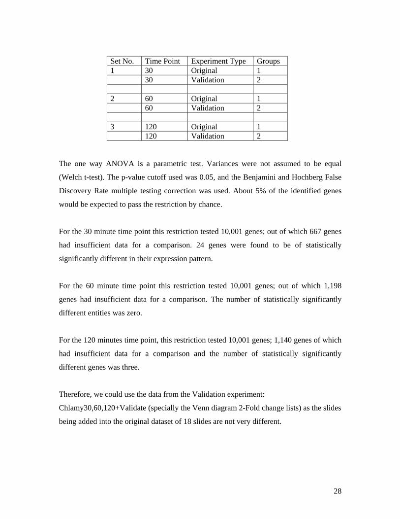
Set No. Time Point Experiment Type Groups 1 30 Original 1 30 Validation 2 2 60 Original 1 60 Validation 2 3 120 Original 1 120 Validation 2

The one way ANOVA is a parametric test. Variances were not assumed to be equal

(Welch t-test). The p-value cutoff used was 0.05, and the Benjamini and Hochberg False

Discovery Rate multiple testing correction was used. About 5% of the identified genes

would be expected to pass the restriction by chance.

For the 30 minute time point this restriction tested 10,001 genes; out of which 667 genes

had insufficient data for a comparison. 24 genes were found to be of statistically

significantly different in their expression pattern.

For the 60 minute time point this restriction tested 10,001 genes; out of which 1,198

genes had insufficient data for a comparison. The number of statistically significantly

different entities was zero.

For the 120 minutes time point, this restriction tested 10,001 genes; 1,140 genes of which

had insufficient data for a comparison and the number of statistically significantly

different genes was three.

Therefore, we could use the data from the Validation experiment:

Chlamy30,60,120+Validate (specially the Venn diagram 2-Fold change lists) as the slides

being added into the original dataset of 18 slides are not very different.

28

There are two types of Venn Diagrams:

1. One labeled ‘Venn’ : This one is made of 2-fold changes lists at 30 min, 60 mins

and 120 mins

2. Second labeled ‘Venn2’: This one is made of 1 way ANOVA T-test lists for 30

min, 60 min and 120 mins

Figure 5: Venn Diagram of 2 Fold Change lists for all 3 time points (30,60,and 120) from GeneSpring GX 9.0 Experiment: Chlamy 30,60,120 Corr

29

Figure 6: Venn Diagram of 2 Fold Change, one way T-test lists for all 3 time points (30, 60, and 120 minutes) from GeneSpring GX 9.0 Experiment: Chlamy30,60,120Corr (Venn2)

Table 1: GeneSpring GX 9.0 Experiment: Chlamy 30,60,120 Corr Summary Data

Time Point No. of Genes (Venn) No. of Genes (Venn2)

30 min 928 80

60 min 2063 85

120 min 1652 79

30

Figure 7: Venn Diagram of 2 Fold Change lists for all 3 time points (30,60,and 120) from GeneSpring GX 9.0 Experiment: Chlamy 30,60,120+Validate

31

Figure 8: Venn Diagram of 2 Fold Change, 1 way T-test lists for all 3 time points (30,60,and 120) (Venn2) from GeneSpring GX 9.0 Experiment: Chlamy30,60,120+Validate

Table 2: GeneSpring GX 9.0 Experiment: Chlamy 30, 60, 120+Validate Summary Data

Time Point No. of Genes (Venn) No. of Genes (Venn2)

30 min 653 101

60 min 1432 123

120 min 1088 122

As can be seen, through the summary tables for both experiments (1 and 2) in

GeneSpring, there is quite a bit of change in the number of genes present in individual

32

time points within both these experiments. We have already proved earlier that data from

the Validation experiment is similar to the data obtained in the original experiment.

The main gene lists extracted through GeneSpring for this project are those of the

individual time point 2 fold change lists and the common genes list within all three time

points. The gene lists used for this project are mainly from the original experiment

“Chlamy30,60,120 Corr” containing 18 slides.

We would although be looking at 2 fold change, gene lists for individual time points as

well as the common gene list within all three time points for both experiments and

making a comparison so as to estimate which genes got eliminated during generation of

the genes lists for the experiment “Chlamy30,60,120+Validate” and the reasons behind

the same.

Several genes related to the photosynthetic machinery such as chloroplast, chlorophyll,

and photosystem I and II related genes were extracted out of these gene lists at each

individual time points as well as in common within all three time points. Several putative

serine threonine protein kinase genes were notable in their response at all three time

points, these enzymes are essential for phosphorylating the LHC-II complex thereby

mobilizing it from PS-II to PS-I causing the state transition [35]. A cell death (apoptosis)

related gene was found to be highly expressed mainly at the 120 minute time point as per

the current Gene Ontology related classification as well as non-updated annotation

information, but there might be several more. These gene lists have been provided in the

Appendix section of this report.

Note: The description column of genes in the following table show, BLAST search

related information and therefore some of the sequences show similarities to sequences

from genus other than Chlamydomonas, such as Arabidopsis thaliana, this is due to the

annotation information being incomplete on the Chlamydomonas genome.

33

Table 3: Some of the photosystem related genes observed within individual time

point gene lists are as follows 30 min Gene

Fold Change Regulation Description

345.A 2.19 up

(-) PHOTOSYSTEM I REACTION CENTRE SUBUNIT III PRECURSOR (LIGHT-HARVESTING COMPLEX I 17 KDA PROTEIN) (PSI-F) (P21 PROTEIN) [Chlamydomonas reinhardtii], 100.0% id

426.A 5.783 up (+) Photosystem II reaction center W protein, chloroplast precursor [Chlamydomonas reinhardtii], 100.0% id

442.A 2.068 up (-) Photosystem I reaction center subunit IV, chloroplast precursor (PSI-E) (Photosystem I 8.1 kDa protein) (P30 protein) [Chlamydomonas reinhardtii], 66.0% id

482.A 2.748 up (+) Photosystem I reaction center subunit II, chloroplast precursor (Photosystem I 20 kDa subunit) (PSI-D) [Chlamydomonas reinhardtii], 100.0% id

69.A 2.296 up (+) Photosystem I reaction center subunit VI, chloroplast precursor (PSI-H) (Light-harvesting complex I 11 kDa protein) (P28 protein) [Chlamydomonas reinhardtii], 100.0% id

8094.D 2.346 up (-) Photosystem I reaction center subunit XI, chloroplast precursor (PSI-L) (PSI subunit V) [Cucumis sativus], 78.3% id

60 min Gene

Fold Change Regulation Description

2850.C 2.171 up (+) (O82660) Photosystem II stability/assembly factor HCF136, chloroplast precursor [Arabidopsis thaliana], 85.6% id

345.A 2.447 up

(-) PHOTOSYSTEM I REACTION CENTRE SUBUNIT III PRECURSOR (LIGHT-HARVESTING COMPLEX I 17 KDA PROTEIN) (PSI-F) (P21 PROTEIN) [Chlamydomonas reinhardtii], 100.0% id

426.A 2.738 up (+) Photosystem II reaction center W protein, chloroplast precursor [Chlamydomonas reinhardtii], 100.0% id

442.A 0.0526 down (-) Photosystem I reaction center subunit IV, chloroplast precursor (PSI-E) (Photosystem I 8.1 kDa protein) (P30 protein) [Chlamydomonas reinhardtii], 66.0% id

69.A 0.269 down (+) Photosystem I reaction center subunit VI, chloroplast precursor (PSI-H) (Light-harvesting complex I 11 kDa protein) (P28 protein) [Chlamydomonas reinhardtii], 100.0% id

120 min Gene

Fold Change Regulation Description

345.A 0.403 down

(-) PHOTOSYSTEM I REACTION CENTRE SUBUNIT III PRECURSOR (LIGHT-HARVESTING COMPLEX I 17 KDA PROTEIN) (PSI-F) (P21 PROTEIN) [Chlamydomonas reinhardtii], 100.0% id

442.A 2.709 up (-) Photosystem I reaction center subunit IV, chloroplast precursor (PSI-E) (Photosystem I 8.1 kDa protein) (P30 protein) [Chlamydomonas reinhardtii], 66.0% id

34

482.A 0.162 down (+) Photosystem I reaction center subunit II, chloroplast precursor (Photosystem I 20 kDa subunit) (PSI-D) [Chlamydomonas reinhardtii], 100.0% id

69.A 2.516 up (+) Photosystem I reaction center subunit VI, chloroplast precursor (PSI-H) (Light-harvesting complex I 11 kDa protein) (P28 protein) [Chlamydomonas reinhardtii], 100.0% id

8094.D 3.971 up (-) Photosystem I reaction center subunit XI, chloroplast precursor (PSI-L) (PSI subunit V) [Cucumis sativus], 78.3% id

Table 4: Some genes of interest from the 160 genes, seen to be commonly expressed

or repressed 2 fold between the three time points are:

Gene Name

30 FC

30 Reg 60 FC 60

Reg 120 FC

120 Reg Description

159.A 4.758 up 0.0424 down 3.185 up

(+) light-harvesting chlorophyll-a/b binding protein Lhcb4 [Chlamydomonas reinhardtii] [Chlamydomonas reinhardtii], 100.0% id

2184.C 0.332 down 3.52 up 0.111 down (-) glbN; cyanoglobin [SP:GLBN_SYNY3] [Synechocystis sp. PCC 6803], 90.3% id

262.A 2.171 up 0.133 down 2.161 up

(+) light-harvesting complex I protein [Chlamydomonas reinhardtii] [Chlamydomonas reinhardtii], 100.0% id

2932.C 5.909 up 4.305 up 4.966 up

(-) Porphobilinogen deaminase, chloroplast precursor (PBG) (Hydroxymethylbilane synthase) (HMBS) (Pre-uroporphyrinogen synthase) [Pisum sativum], 81.3% id

345.A 2.19 up 2.447 up 0.403 down

(-) PHOTOSYSTEM I REACTION CENTRE SUBUNIT III PRECURSOR (LIGHT-HARVESTING COMPLEX I 17 KDA PROTEIN) (PSI-F) (P21 PROTEIN) [Chlamydomonas reinhardtii], 100.0% id

361.A 4.256 up 0.428 down 3.923 up

(+) Delta-aminolevulinic acid dehydratase, chloroplast precursor (Porphobilinogen synthase) (ALADH) [Chlamydomonas reinhardtii], 100.0% id

371.A 2.838 up 15.6 up 0.156 down

(+) light harvesting complex I protein precursor [Chlamydomonas reinhardtii] [Chlamydomonas reinhardtii], 100.0% id

442.A 2.068 up 0.0526 down 2.709 up

(-) Photosystem I reaction center subunit IV, chloroplast precursor (PSI-E) (Photosystem I 8.1 kDa protein) (P30 protein) [Chlamydomonas reinhardtii], 66.0% id

35

444.A 6.65 up 0.349 down 3.569 up

(-) Ribulose-phosphate 3-epimerase, chloroplast precursor (Pentose-5-phosphate 3-epimerase) (PPE) (RPE) (R5P3E) [Spinacia oleracea], 82.8% id

5661.C 2.078 up 2.647 up 19.1 up (-) (Q9LYR5) Thylakoid lumenal 18 kDa protein, chloroplast precursor [Arabidopsis thaliana], 78.1% id

69.A 2.296 up 0.269 down 2.516 up

(+) Photosystem I reaction center subunit VI, chloroplast precursor (PSI-H) (Light-harvesting complex I 11 kDa protein) (P28 protein) [Chlamydomonas reinhardtii], 100.0% id

8255.D 0.253 down 2.123 up 9.344 up (+) CALK protein [Chlamydomonas reinhardtii] [Chlamydomonas reinhardtii], 100.0% id

8711.D 4.131 up 0.455 down 2.092 up (+) (Q38833) Putative chlorophyll synthetase (G4) [Arabidopsis thaliana], 83.2% id

8815.D 0.314 down 9.886 up 9.985 up (+) Tbc2 translation factor, chloroplast precursor [Chlamydomonas reinhardtii], 90.7% id

8923.E 2.008 up 2.046 up 2.512 up

(-) (Q9ASS6) Peptidyl-prolyl cis-trans isomerase TLP20, chloroplast precursor (EC 5.2.1.8) (PPIase) (Rotamase) (Thylakoid lumen PPIase of 20 kDa) [Arabidopsis thaliana], 64.5% id

9538.E 2.142 up 0.286 down 2.924 up (-) chlorophyll a/b-binding protein [Chlamydomonas reinhardtii] [Chlamydomonas reinhardtii], 92.3% id

9853.E 3.031 up 0.291 down 3.791 up (-) 50S RIBOSOMAL PROTEIN L13, CHLOROPLAST PRECURSOR (CL13) [Spinacia oleracea], 58.4% id

As seen from the table above, most of the genes are seen to follow an “up-down-up”

regulation pattern (induction-repression-induction). The PS-I reaction center subunit-III

precursor protein related gene (345.A) is seen to be induced through the first one hour

and later repressed towards the end of the 2nd hour. The LHC-I protein precursor related

gene (371.A) is also seen to be induced during the first one hour and is later repressed

towards the end of the second hour. The LHC-I protein gene (262.A) is accordingly seen

to be induced during the first 30 minutes, and later repressed at the 60 minute time point

and then again induced towards the end of the 2 hour time point exactly alternating with

it’s precursor protein related gene.

36

The LHC-I (P28 protein) related gene (69.A) is seen to follow the “up-down-up” pattern

along with the LHC chlorophyll a/b binding protein Lhcb4 (159.A) and the PS-I reaction

center subunit IV chloroplast precursor protein (442.A). The PS-I reaction center subunit

III precursor (345.A) is seen induced in the first one hour and repressed toward the end of

the 2nd hour.

The CALK protein (8255.D) gene is seen to be repressed in the first half an hour and later

seen to be induced incrementally from the 1 hour to the 2 hour time point. This is an

aurora protein kinase said to be involved in the regulated flagellar disassembly pathway

as well as flagellar autotomy in Chlamydomonas[34]. There is a theory about

Chlamydomonas possessing sensory pathways so as to detect inappropriate conditions in

its environment whereby they disassemble organelles like their flagella which aren’t

absolutely necessary for survival in an attempt to adapt to the changed environment. In

our experiment we place the photosynthetic alga Chlamydomonas in the dark which is

not an ideal environment for photosynthesis, and data from our microarray experiment

suggests a rise in the CALK gene beginning the one hour time point with an increasing

trend towards the end of the 2nd hour re-verifying data published in research by Pan et.al.

(2004) [34].

Several such conclusions may be drawn from this experimental data, but they need to be

backed by either previous biochemical or genetic experimental data or new experiments

need to be performed in those directions.

37

Future Work – Recommendations

The microarray data from this project is being validated using quantitative polymerase

chain reaction data for some of the candidate genes extracted through the gene lists

presented in this report. This PCR data will be compared with the data obtained from the

microarray quantitatively as well using GeneSpring.

Since the Chlamydomonas microarray slides used for this project are custom arrays, the

annotations of all the array elements have not been updated as per recent

Chlamydomonas annotation information within the .gal file provided with the array.

Also, Gene Ontology related information is incomplete and has not been included in the

.gal file, therefore sorting of genes as per function is at the moment, partly, a manual task

through Microsoft excel sorting methods.

Some of the future work towards this project would involve updating this annotation

related information through BLAST search into the .gal file. Various other gene lists can

be extracted through different parsing algorithms of GeneSpring and analysis of the same

will be done for both the individual time points as well as common expression within all

three time points.

We would also, implement some automation in the process of gene list sorting based on

function so as to better help elucidate the final model of gene expression changes

occurring during the state1 to state2 transition. Based upon results obtained from this

experiment, more time points may be added to this study. Gene expression change data

from this project would also be clubbed together with protein structure and expression

data for a better understanding of the molecular change occurring in the state1 to state2

transition.

38

References

1. Florence Mus, Alexandra Dubini, Michael Seibert, Matthew C. Posewitz, and Arthur R. Grossman. (2007) Anaerobic Acclimation in Chlamydomonas reinhardtii: Anoxic Gene Expression, Hydrogenase Induction, and Metabolic Pathways. J. Biol.Chem. 282: 25475-25486.

2. Fouchard, S., Hemschemeier, A., Caruana, A., Pruvost, J., Legrand, J., Happe, T., et al. (2005). Autotrophic and mixotrophic hydrogen photoproduction in sulfur-deprived chlamydomonas cells. Applied and Environmental Microbiology, 71(10), 6199-6205.

3. Jeanette M. Quinn, Mats Eriksson, Jeffrey L. Moseley, and Sabeeha Merchant

(2002). Oxygen Deficiency Responsive Gene Expression in Chlamydomonas reinhardtii through a Copper-Sensing Signal Transduction Pathway Plant Physiology. 128: 463-471.

4. Zhang et al. (2004).Insights into the Survival of Chlamydomonas reinhardtii

during Sulfur Starvation Based on Microarray Analysis of Gene Expression Eukaryotic Cell, 3: 1331

5. Ruohui Xu, Scott E. Bingham and Andrew N. Webber (1993). Increased mRNA

accumulation in a psaB frame-shift mutant of Chlamydomonas reinhardtii suggests a role for translation in psaB mRNA stability, Plant Molecular Biology 22: 465-474.

6. Rajagopal Subramanyam, Craig Jolley, Daniel C. Brune, Petra Fromme and

Andrew N. Webber (2006). Characterization of a novel Photosystem I–LHCI supercomplex isolated from Chlamydomonas reinhardtii under anaerobic (State II) conditions. FEBS Letters Volume 580, Issue 1, Pages 233-238.

7. Ramesh, V, Bingham, SE, and Webber, AN (2004). A simple method for

chloroplast transformation in C. reinhardtii. Methods in Molecular Biology 274: 301-307.

8. Elizabeth H. Harris (1989). The Chlamydomonas Source Book. Academic

Press.

9. J.D. Rochaix, M Goldschmidt, S. Merchant (1998). The Molecular Biology of Chloroplasts and Mitochondria in Chlamydomonas. Published by Springer.

10. Mohammad Pessarakli (2005). Handbook of Photosynthesis, Chapter 16:

Regulation of Photosynthesis by Protein Phosphorylation: State 1 and 2 Transitions – George S. Bullerjahn. Published by Marcel Dekker, Pages 257-267.

39

11. Greg Gibson & Spencer V. Muse (2004). A primer of Genome Science, 2nd Ed.,

Sinauer Associates, Inc. Publishers, 12. Richard J. Reece (2004). Analysis of Genes and Genomes, Wiley Publications,

2004.

13. Douglas C. Montgomery (2005). Design and Analysis of Experiments, 6th Ed., Wiley Publications.

14. Sorin Draghici (2003). Data Analysis Tools for DNA Microarrays, Chapman &

Hall.

15. Jacob Cohen, Patricia Cohen, Stephen G. West, Leona S. Aiken (2003), Applied Multiple Regression/Correlation Analysis for the Behavioral Sciences (3rd Ed.), Lawrence Erlbaum Associates, Publishers.

16. GeneSpring GX 7.3.1 and 9.0 User Manuals – Agilent Technologies.

17. GenePix Pro 6.0 Microarray Acquisition and Analysis Software for GenePix

Microarray Scanners User’s Guide & Tutorial (2005). Axon Instruments/ Molecular Devices Corp.

18. GenePix Microarray Scanner Manual – Axon Instruments/ Molecular Devices

Corp.

19. Agilent - G2565BA Microarray Scanner User Manual – Agilent Technologies.

20. Agilent - RNA 6000 Nano Kit Quick Start Guide.

21. Invitrogen - TRIzol Plus RNA Purification Kit.

22. Qiagen - RNeasy Mini Protocol for RNA Cleanup.

23. Ambion - Amino Allyl MessageAmp II aRNA Amplification Protocol: http://www.ambion.com/catalog/ProdGrp.html?fkProdGrp=341

24. Fermentas Protocol for the Removal of Template DNA Following in vitro

Synthesis of RNA (with DNase I, RNase-free). http://www.fermentas.com/techinfo/modifyingenzymes/protocols/p_elimdna.htm

25. Fermentas Protocol for Preparation of DNA-free RNA Prior to RT-PCR

(with DNase I, RNase-free). http://www.fermentas.com/techinfo/modifyingenzymes/protocols/p_prepdnafreerna.htm

40

26. Oligoarray Protocol – Stephen Eberhard (2005).

http://www.chlamy.org/protocol.doc 27. University of Arizona, College of Agriculture and Life Sciences, Arabidopsis

Microarray Target Preparation and Hybridization Protocol. http://ag.arizona.edu/microarray/Microarraymethod1.doc

28. Ambion - Amino Allyl MessageAmp II aRNA Amplification Calculator Link:

http://www.ambion.com/techlib/append/mm_calcs/aamsgamp2_calc.php

29. Chlamydomonas Center Website - Duke University: http://www.chlamy.org/

30. Lowess Normalization Reference: http://stat-www.berkeley.edu/users/terry/zarray/Html/normspie.html.

31. Giorgio Forti, and Giovanni Caldiroli (2005), State Transitions in

Chlamydomonas reinhardtii. The Role of the Mehler Reaction in State 2-to-State 1 Transition. Plant Physiol. 137: 492-499.

32. Giovanni Finazzi (2005), The central role of the green alga Chlamydomonas

reinhardtii in revealing the mechanism of state transitions. J. Exp. Bot. 56: 383-388.

33. Giovanni Finazzi, Romina Paola Barbagallo, Elena Bergo, Roberto Barbato, and

Giorgio Forti, Photoinhibition of Chlamydomonas reinhardtii in State 1 and State 2. DAMAGES TO THE PHOTOSYNTHETIC APPARATUS UNDER LINEAR AND CYCLIC ELECTRON FLOW, J. Biol. Chem. 276: 22251-22257.

34. J. Pan, Q. Wang, W. Snell (2004). An Aurora Kinase Is Essential for Flagellar

Disassembly in Chlamydomonas. Developmental Cell, Volume 6, Issue 3, Pg. 445 - 451.

35. Nathalie Depège, Stéphane Bellafiore, and Jean-David Rochaix (2003).Role of

Chloroplast Protein Kinase Stt7 in LHCII Phosphorylation and State Transition in Chlamydomonas. Science 299: (5612), 1572.

41

Appendix

A list of genes, as shown in Tables 4 and 5, obtained from this analysis, included along with this report.

42