Embed Size (px)
Citation preview

Cognitive Psychology 42, 317–367 (2001)
doi:10.1006/cogp.2001.0750, available online at http://www.idealibrary.com on
Time Course of Frequency Effects in Spoken-WordRecognition: Evidence from Eye Movements
Delphine Dahan, James S. Magnuson, and Michael K. Tanenhaus
University of Rochester
In two experiments, eye movements were monitored as participants followed spo-ken instructions to click on and move pictures with a computer mouse. In Experi-ment 1, a referent picture (e.g., the picture of a bench) was presented along withthree pictures, two of which had names that shared the same initial phonemes asthe name of the referent (e.g., bed and bell). Participants were more likely to fixatethe picture with the higher frequency name (bed) than the picture with the lowerfrequency name (bell). In Experiment 2, referent pictures were presented with threeunrelated distractors. Fixation latencies to referents with high-frequency names wereshorter than those to referents with low-frequency names. The proportion of fixa-tions to the referents and distractors were analyzed in 33-ms time slices to providefine-grained information about the time course of frequency effects. These analysesestablished that frequency affects the earliest moments of lexical access and ruleout a late-acting, decision-bias locus for frequency. Simulations using models inwhich frequency operates on resting-activation levels, on connection strengths, andas a postactivation decision bias provided further constraints on the locus of fre-quency effects. 2001 Academic Press
Key Words: lexical frequency; spoken-word recognition; eye tracking.
As the sound pattern of a spoken word unfolds over time, recognitiontakes place against a backdrop of partially activated alternatives that competefor recognition. The most activated alternatives are those that most closelymatch the input. For instance, as a listener hears the word cap, lexical repre-sentations of words with similar sounds, such as cat, will be briefly activated.
This work was supported by NSF Grant SBR-9729095 to Michael K. Tanenhaus and Rich-ard N. Aslin, and an NSF GRF to James S. Magnuson. We thank Ellen Hogan for her helpin constructing the materials and Ellen Hogan, Sarah Scheidel, and Dana Subik for their helpin testing participants. We thank Paul Allopenna, Mark Pitt, and Uli Frauenfelder for technicaladvice on the TRACE model. Helpful comments from Fernanda Ferreira led to some of theanalyses presented in Experiment 1. We thank her and three anonymous reviewers for sugges-tions that improved this article.
Address correspondence and reprint requests to Delphine Dahan, Max-Planck Institute forPsycholinguistics, Postbus 310, 6500 AH Nijmegen, The Netherlands. Fax: (31) 24 352 1213.E-mail: [email protected].
3170010-0285/01 $35.00
Copyright 2001 by Academic PressAll rights of reproduction in any form reserved.

318 DAHAN, MAGNUSON, AND TANENHAUS
The number of competitors, their frequency of occurrence in the language,as well as the frequency of occurrence of the target word itself all affectrecognition (e.g., Luce & Pisoni, 1998; Marslen-Wilson, 1987, 1990). Thepresent study focuses on the time course of frequency effects for words andtheir close competitors.
A variety of response measures has established that recognition of low-frequency words is poorer than recognition of high-frequency words (e.g.,Howes & Solomon, 1951). Superior performance on high-frequency wordsmay be observed either in the speed of the response when the stimulus infor-mation is sufficient to support accurate performance, as in most reaction-time paradigms (e.g., Marslen-Wilson, 1987) or in the accuracy of the re-sponse when the stimulus is degraded (e.g., Luce, 1986; Goldinger, Luce, &Pisoni, 1989).
In most current models of spoken-word recognition, frequency is assumedto affect the activation levels of competing lexical candidates during lexicalaccess. For example, in models with discrete lexical representations such asthe ‘‘Cohort’’ model (Marslen-Wilson, 1987) or the TRACE model (McClel-land & Elman, 1986), high-frequency words would be processed faster thanlow-frequency words because frequency determines either the baseline acti-vation level of each lexical unit (McClelland & Rumelhart, 1981; Marslen-Wilson, 1990) or the strength of the connections from sublexical to lexicalunits (MacKay, 1982, 1987). In distributed learning models, the representa-tions of high-frequency words would be activated more rapidly because high-frequency mappings are better learned, resulting in stronger connectionweights (Gaskell & Marslen-Wilson, 1997; Plaut, McClelland, Seiden-berg, & Patterson, 1996). In contrast, the Neighborhood Activation Model(henceforth, NAM; Luce, 1986; Luce & Pisoni, 1998) places the locus offrequency effects in a decision stage that follows initial lexical activation.In this model, the input stimulus activates a set of acoustic–phonetic patternsthat shares some degree of similarity with the input; these acoustic–phoneticpatterns in turn activate word-decision units that are tuned to them. High-level information, such as word frequency, is associated with each word-decision unit. Acoustic–phonetic information is assumed to drive the systemby activating word-decision units, whereas high-level lexical information isassumed to operate by biasing these decision units. Frequency bias operatesby adjusting the activation levels represented within the word-decision units.Thus, word frequency is not directly coded in the resting-activation level,but rather operates as a bias on the activation of the word-decision unit.Nonetheless, frequency comes into play before lexical access is completed.
An alternative hypothesis about the locus of frequency effects in wordrecognition has been suggested by Balota and Chumbley (1984, 1985). Theyargued that the facilitation for responding to high-frequency words comparedto low-frequency words in a task such as visual lexical decision mostly re-flects a response bias that operates at a decision stage. Similarly, word-

FREQUENCY AND EYE TRACKING 319
frequency effects in a pronunciation task (i.e., naming a word visually dis-played) are attributed to the word-production process, which is presumed tofollow lexical access. This conception of frequency as a response bias ap-pears similar to the decision bias incorporated in the NAM. However, itfurther assumes that frequency effects occur late in processing, as a responsebias that affects decisions after lexical access is completed.
The locus of frequency effects has been widely debated in the visual-wordrecognition and naming literature (e.g., Balota & Chumbley, 1990; Monsell,Doyle, & Haggard, 1989; see Monsell, 1991, for a review). Paap and col-leagues (Paap, Newsome, McDonald, & Schvaneveldt, 1982; Paap &Johansen, 1994) argued that frequency effects occur during a verificationphase, following the initial activation phase. However, this claim has beenchallenged by Allen and colleagues (Allen, McNeal, & Kvak, 1992; Allen,Smith, Lien, Weber, & Madden, 1997). Models adopting a distributed repre-sentation of word knowledge, however, do not assume distinct stages duringword recognition, such as pre- or postlexical access stages (e.g., Seiden-berg & McClelland, 1989; Plaut et al., 1996). Such models show sensitivityto word frequency because words that are presented more often during train-ing have a larger impact on the settings of the connection weights (seeMcCann & Besner, 1987, for a similar proposal). Thus, frequency can affectmultiple levels in the system: In a naming task, it affects both the compu-tation of the phonological code and the conversion of the computed phono-logical code into a sequence of articulatory-motor commands (see McRae,Jared, & Seidenberg, 1990).
Although subject to intense debate in the visual-word recognition litera-ture, the locus of frequency effects has received less attention in the spoken-word recognition literature. Of particular interest are studies by Marslen-Wilson (1987) and Zwitserlood (1989). In these studies, a spoken-word frag-ment that matched both a high-frequency and a low-frequency lexical candi-date was presented, followed shortly by the visual presentation of a targetword; participants were instructed to perform a lexical decision on the visualtarget. The results revealed less facilitation (compared to a control) for targetwords semantically associated with the low-frequency candidate than for tar-get words associated with the high-frequency candidate. This was interpretedas evidence that the higher frequency candidate becomes more activated thanthe lower frequency candidate before the auditory input could distinguishbetween the two. However, Connine, Titone, and Wang (1993) argued thatbecause the input was incomplete, subjects implicitly completed the inputwith the more frequent alternative on a greater proportion of the trials; thiswould lead to a larger priming effect for the more frequently generated alter-native. On this account, frequency is being used to bias selection of the higherfrequency alternative rather than its activation. The same argument can beapplied to studies demonstrating word-frequency effects using the gating par-adigm (Grosjean, 1980; Tyler, 1984).
320 DAHAN, MAGNUSON, AND TANENHAUS
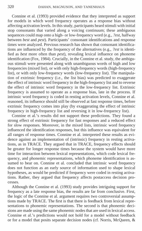
Connine et al. (1993) provided evidence that they interpreted as supportfor models in which word frequency operates as a response bias withoutaffecting activation levels. In this study, participants heard stimuli with initialstop consonants that varied along a voicing continuum; these ambiguoussequences could map onto a high- or low-frequency word (e.g., ?est, halfwaybetween best and pest). Participants’ consonant identifications and responsetimes were analyzed. Previous research has shown that consonant identifica-tions are influenced by the frequency of the alternatives (e.g., ?est is identi-fied as best more often than pest), revealing lexical influence on phonemeidentification (Fox, 1984). Crucially, in the Connine et al. study, the ambigu-ous stimuli were presented along with unambiguous words of high and lowfrequencies (mixed list), or with only high-frequency words (high-frequencylist), or with only low-frequency words (low-frequency list). The manipula-tion of extrinsic frequency (i.e., the list bias) was predicted to exaggeratethe effect of intrinsic word frequency in the high-frequency list and to reversethe effect of intrinsic word frequency in the low-frequency list. Extrinsicfrequency is assumed to operate as a response bias, late in the process. Ifintrinsic word frequency is coded in resting activation levels, Connine et al.reasoned, its influence should still be observed at fast response times, beforeextrinsic frequency comes into play (by exaggerating the effect of intrinsicfrequency in high-frequency list and reversing it in low-frequency list).
Connine et al.’s results did not support these predictions. They found astrong effect of extrinsic frequency for fast responses and a reduced effectfor slow responses. Moreover, in the mixed lists, intrinsic word frequencyinfluenced the identification responses, but this influence was equivalent forall ranges of response times. Connine et al. interpreted these results as evi-dence against an implementation of (intrinsic) frequency in resting activa-tions, as in TRACE. They argued that in TRACE, frequency effects shouldbe greater for longer response times because the system would have moretime for interaction between lexical representations, which code lexical fre-quency, and phonemic representations, which phoneme identification is as-sumed to bear on. Connine et al. concluded that intrinsic word frequencydoes not function as an early source of information used to shape lexicalhypotheses, as would be predicted if frequency were coded in resting activa-tions. Rather, they argued that frequency affects postaccess decision pro-cesses.
Although the Connine et al. (1993) study provides intriguing support forfrequency as a late response bias, the results are far from conclusive. First,the logic of the Connine et al. argument requires two controversial assump-tions made by TRACE. The first is that there is feedback from lexical repre-sentations to phonemic representations. The second is that phonemic deci-sions are made using the same phonemic nodes that are used in lexical access.Connine et al.’s predictions would not hold for a model without feedbackor for a model that posits separate decision nodes (cf. Norris, McQueen, &

FREQUENCY AND EYE TRACKING 321
Cutler, 2000). Furthermore, Connine et al.’s arguments are based on verbalpredictions rather than actual simulations with TRACE. Thus, it is difficultto know under just what conditions the predictions hold. Making predictionswithout simulations is not straightforward without explicit assumptionsabout how to relate the time course of lexical-activation levels and fast andslow response latencies in phoneme identification. Finally, McQueen (1991)found larger lexical influences on fast phoneme-identification times than onslower identification times. This can be interpreted either as evidence againstfeedback between lexical and phonemic levels or as evidence that phoneme-identification latencies do not capture the time course of lexical influenceon phoneme activation: By the time fast responses are generated, lexicalfeedback to phonemic nodes may have largely taken place; lexical influenceon slow latencies may be masked by the influence of late decision biasesspecific to the task or activations reaching asymptotic levels. Regardless ofhow McQueen’s results are interpreted, they suggest that using phoneme-identification times to track the time course of lexically based frequencyeffects is not straightforward.
The issues raised by the Connine et al. (1993) study highlight the impor-tance of having precise information about the time course of activation forlexical competitors in order to identify where, in the recognition process,word frequency operates. Although researchers have developed an arsenalof useful experimental methodologies (see Grosjean & Frauenfelder, 1996;Lively, Pisoni, & Goldinger, 1994), it remains difficult to obtain data aboutlexical access in continuous speech that is fine-grained enough to favor oneword-frequency account against the others. The presentation of increasinglylonger word fragments to measure the degree of activation of high- and low-frequency competitors (Grosjean, 1980; Tyler, 1984; Zwitserlood, 1989)aims at providing a continuous measure of lexical activation. However,because it is quite remote from normal listening conditions, this techniquemay cause listeners to adopt strategies that might not reflect normal lexicalaccess.
A growing number of researchers, building on work by Cooper (1974),have recently begun to use eye movements to explore questions about thetime course of spoken-language comprehension (e.g., Altmann & Kamide,1999; Eberhard, Spivey-Knowlton, Sedivy, & Tanenhaus, 1995; Keysar,Barr, Balin, & Brauner, 2000; Tanenhaus & Spivey-Knowlton, 1996; Tanen-haus, Spivey-Knowlton, Eberhard, & Sedivy, 1995; Trueswell, Sekerina,Hill, & Logrip, 1999). In the version of the eye-tracking paradigm introducedby Tanenhaus et al. (1995), participants follow spoken instructions to manip-ulate real or pictured objects displayed on a computer screen while their eyemovements to the objects are monitored using a lightweight camera mountedon a head band. Eye movements to objects in the visual scene have beenfound to be closely time-locked to referring expressions in the unfoldingspeech stream.

322 DAHAN, MAGNUSON, AND TANENHAUS
Allopenna, Magnuson, and Tanenhaus (1998) explored the application ofthis technique to the study of spoken-word recognition. Participants wereinstructed to fixate a central cross and then followed a spoken instruction tomove (using a computer mouse) one of four objects displayed on a computerscreen (e.g., ‘‘Look at the cross. Pick up the beaker. Now put it above thesquare’’). Eye movements to each of the objects were recorded as the nameof the referent object unfolded over time. On some crucial trials, the namesof some of the distractor objects were phonologically similar to the nameof the referent. For instance, the target picture beaker was presented withthe picture of a competitor that overlapped with the target word at onset,beetle (henceforth, a cohort competitor, predicted to compete by the ‘‘Co-hort’’ model, e.g., Marslen-Wilson & Welsh, 1978). The probability of fixat-ing each object as the target word was heard was hypothesized to be closelylinked to the activation of the lexical representation of this object (i.e., itsname). The assumption providing the link between lexical activation and eyemovements is that the activation of the name of a picture influences theprobability that a subject will shift attention to that picture and thus makea saccadic eye movement to fixate it.
Allopenna et al. (1998) showed that eye movements generated early inthe target word were equally likely to result in fixations to the cohort compet-itor (e.g., beetle) and to the referent (e.g., beaker) and were more likelyto result in fixations to these pictures than to distractor controls that werephonologically unrelated to the target word (e.g., carriage). Furthermore,the fixations over time to the target, the cohort competitor, and a rhymecompetitor (e.g., speaker) closely matched functions generated by theTRACE model of spoken-word recognition, given a simple implementationof the hypothesis linking activation levels in TRACE to fixation probabilitiesover time. The Allopenna et al. study suggests that the eye-tracking paradigmis a powerful tool for providing detailed time-course information about lexi-cal access in continuous speech. The timing of frequency effects as revealedby fixations should be informative about whether word-frequency operatesearly in processing, when the input is still ambiguous among multiple lexicalalternatives, or late in processing, after the input has converged on a singlelexical candidate. Furthermore, the explicit linking hypothesis between lexi-cal activation and observed fixations allows for quantitative comparisons ofthe goodness of fit between the observed and predicted fixations when wordfrequency is implemented in resting activations, in connection strengths, oras a bias in computing the activation of word-decision units.
Examination of frequency effects is also important for evaluating the gen-eral usefulness of the eye-tracking paradigm. In this paradigm, a small setof pictures is visually available to the listener. Participants could be adoptingtask-specific strategies that bypass ‘‘normal’’ language comprehension (e.g.,preactivating the names of the visually present pictures). Thus, it is possiblethat the lexical candidates that enter the recognition process may be restricted

FREQUENCY AND EYE TRACKING 323
to the visually present alternatives. Previous research has shown that well-documented frequency and neighborhood effects in word recognition can bedramatically reduced or even disappear in closed-set tests when all responsealternatives are treated as equally probable (Pollack, Rubenstein, & Decker,1959; Sommers, Kirk, & Pisoni, 1997). Thus, it remains to be establishedwhether the eye-tracking paradigm is sensitive to characteristics of the lexi-con that are not directly represented in the set of pictures displayed on atrial. The answer bears directly on the hypothesis linking lexical activationto eye movements and on the overall potential of the methodology for study-ing word recognition in continuous speech.
The present study had three goals. First, we asked whether the eye-trackingparadigm could capture subtle aspects of word processing such as word-frequency effects. Second, by analyzing the time course of the frequencyeffects on fixations, we evaluated two alternative accounts for the locus offrequency effects: the response-bias account which predicts late frequencyeffects, as suggested by Balota and Chumbley (1984, 1985) and Connine etal. (1993), and an account of frequency as part of the word-recognition sys-tem which predicts that frequency affects even the earliest moments of lexi-cal activation. Finally, we implemented frequency in three ways (frequencyin resting activation, frequency in connection strengths, and frequency as apostactivation bias) and compared the goodness of fit between the predictedfixations generated by these models and the data. These simulations evalu-ated whether these different models would yield different quantitativeand/or qualitative predictions and whether the data would favor one overthe others.
In Experiment 1, we presented participants with displays consisting of areferent along with two cohort competitors that varied in frequency and anunrelated distractor. For example, the referent bench was presented alongwith a high-frequency competitor, bed; a low-frequency competitor, bell;and a distractor, lobster. Participants were instructed to pick up the desig-nated object by clicking on it with the computer mouse (e.g., ‘‘Pick up thebench’’). As the initial sounds of the target word were heard, the competitorswere expected to be fixated more than the distractor as a consequence oftheir phonological similarity with the initial portion of the input. In addition,if fixations reflect lexical processing, more fixations to the high-frequencycompetitor than to the low-frequency competitor would be expected. Cru-cially, if lexical frequency operates on the lexical-access process (rather thanas a possible response bias), the advantage for fixating the high-frequencycompetitor over the low-frequency competitor should be observed before theauditory input provides disambiguating information.
Finding a frequency effect on the fixations to visually present competitorswould demonstrate that participants do not treat them as equally probablereferents. However, finding such effect does not preclude the possibility thatparticipants adopt some sort of verification strategy that does not reflect nor-

324 DAHAN, MAGNUSON, AND TANENHAUS
mal spoken-word processing. In particular, participants could name the visu-ally present pictures to themselves before hearing the referent’s name andstore these names in short-term memory; frequency could bias the order inwhich the preactivated names are stored and/or retrieved. Experiment 2 eval-uated whether an effect of frequency could be obtained when none of thedistractors was phonologically similar to the target. We varied the frequencyof the names of the referents (e.g., the high-frequency target horse vs the low-frequency target horn) and presented them along with three phonologicallyunrelated distractors. The referent picture was thus the only picture with aname matching the target word. If the probability of fixating a picture reflectsactivation of the lexical representation associated with this picture, fixationsshould be made to referent pictures with high-frequency names faster thanto referent pictures with low-frequency names because high-frequency wordsare activated faster than low-frequency words. Accounting for such a fre-quency effect by a verification strategy due to previewing the pictures beforeany relevant information is heard is not tenable, as we discuss later.
EXPERIMENT 1
Method
Participants
Twenty native speakers of English were recruited at the University of Rochester and paid$7.50 for their participation.
Materials
Seventeen triplets were constructed. Each consisted of a target and two cohort competitors.Cohort competitors were chosen in such a way that they overlapped with the target’s phonolog-ical form to the same extent, but differed in lexical frequency (as reported in Francis & Kucera,1982). For example, one target was bench, with the high-frequency competitor bed (with afrequency of 139 per million) and the low-frequency competitor bell (with a frequency of 23per million). For one triplet, bandaid/bank/banjo, the low-frequency competitor overlappedwith the target word more than the high-frequency competitor did. The complete set of tripletsis presented in Appendix A, set A. On average, the high-frequency competitor had a frequencyof 138 per million; the low-frequency competitor, 10 per million; and the target, 14.5 permillion. Each triplet was associated with a phonologically unrelated distractor (e.g., lobster).In addition to these 17 experimental displays, 23 filler displays were constructed. In order toprevent participants from developing expectations that pictures with phonologically similarnames were likely to be targets, 8 of the filler trials contained three items that started withsimilar sounds and a phonologically unrelated item, which was the target. The 15 other fillertrials were composed of four phonologically unrelated items; three of them were presentedat the beginning of the session to familiarize participants with the task and the procedure.
The 160 pictures [(17123) trials 3 4 pictures] were all black-and-white line drawings.They were selected from the Snodgrass and Vanderwart (1980) picture set as well as fromchildren’s picture dictionaries. In order to ensure that the pictures associated with high- andlow-frequency items were equally identifiable, we presented the pictures to 18 participants

FREQUENCY AND EYE TRACKING 325
and asked them to write the name of the object represented. We thus collected names for the34 cohort-item pictures. A correct response was an answer that exactly corresponded to theintended name or this name preceded or followed by a modifier. So, shopping cart for theintended cart was coded as a correct response, but chest for the intended trunk was not. Theagreement between participants’ responses and the intended names was 91.4% for the low-frequency cohorts and 90.1% for the high-frequency cohorts.
Despite similar name agreement for high- and low-frequency items, it was important tocontrol for possible visual differences. Indeed, if the pictures associated with high-frequencycompetitors attracted more attention than the pictures associated with low-frequency competi-tors, more and longer fixations to the former compared to the latter would be found and mistak-enly interpreted as a frequency effect. We thus needed, for each type of competitors, an esti-mate of fixation probability that was independent of their phonological similarity with thetarget word. We thus constructed another set of experimental trials and fillers (set B). Theexperimental trials consisted of the same items except for the target, which was phonologicallyunrelated to the cohorts or to the distractor (e.g., mushroom was one target, presented alongwith bed, bell, and lobster, and participants heard the instruction ‘‘Pick up the mushroom’’).These trials allowed us to compare the probability of fixating each cohort item when neithermatched the acoustic information of the target word. These probabilities should be triggeredby the visual characteristics of the pictures. In order to prevent strategies for finding a trial’starget on the basis of phonological similarity between the pictured items, we constructed 13filler trials where two items shared some similarity and one of them was the target. The materi-als for set B are presented in Appendix A. Ten participants were randomly assigned to eachdisplay set.1 For each set, five random orders were created; approximately the same numberof participants were assigned to each order.
The spoken instructions were recorded by a male native speaker of English in a soundproofroom, sampling at 22,050 Hz with 16-bit resolution. Each instruction was then edited and somebasic duration measurements were made. On average, the pick up the part of the instruction was402 ms long in set A and 371 ms in set B; the target word was 498 ms long in set A and497 ms in set B.
Procedure
Participants were seated at a comfortable distance from the computer screen. Participants’eye movements were monitored using an Applied Scientific Laboratories eye tracker. Twocameras mounted on a lightweight headband provided the input to the tracker. The eye cameraprovided an infrared image of the eye. The center of the pupil and the first Purkinje image(corneal reflection) were tracked to determine the position of the eye relative to the head. Ascene camera was aligned with the participant’s line of sight. A calibration procedure allowedsoftware to superimpose crosshairs showing the point of gaze on a HI-8 videotape record ofthe scene camera. The scene camera sampled at a rate of 30 frames per second, and eachframe was stamped with a time code. Auditory stimuli were played to the subject throughheadphones and simultaneously to the HI-8 VCR, providing an audio record of each trial.Two different computers were used to present the visual and the auditory stimuli on each trial,and the experimenter synchronized these two events by pressing both keyboards simulta-neously. Note that timing measurements were made independently of the accuracy of thissynchronization because speech and eye movements were assessed directly from the videorecording. Any variability in this synchronization resulted only in slight variance in the delaybetween the presentation of the pictures and the onset of the spoken instruction.
1 Each participant was actually exposed to both sets and the order of presentation of thesets was varied between participants; however, we only analyzed the trials for the first setpresented.

326 DAHAN, MAGNUSON, AND TANENHAUS
The structure of each trial was as follows: First, a 5 3 5 grid with a centered cross appearedon the screen, and participants were instructed to look at the cross and to click on it. Thisallowed the experimenter to check that the calibration of the eye tracker was satisfactory.(Note that this instruction was given before the pictures were displayed, and participants werenot instructed to fixate the cross at any other moment during the trial). Four line-drawingpictures and four colored geometric shapes appeared on specific cells of the grid. Participantswere seated between 40 and 60 cm from the screen; each cell in the grid subtended 3° to 4°of visual angle, which is well within the resolution of the tracker (better than 1°). Approxi-mately 500 ms after the pictures appeared, the spoken instruction started. The format of theinstruction was constant across all trials: Participants were first asked to pick up one of thefour pictures using the computer mouse (e.g., ‘‘Pick up the bench.’’) and then to move thepicture above or below one of the four geometric shapes (‘‘Put it above/below the circle/square/diamond/triangle.’’). Once this was accomplished, the next trial began. The positionsof the geometric shapes were fixed from one trial to the next. The position of each picturewas randomized for each subject and each trial.
To minimize participants’ prior exposure to the pictures, we departed from the procedureused in Allopenna et al. (1998) in two ways. First, the set of pictures was not shown to theparticipants before the experiment. Second, Allopenna et al. gave participants approximately2 s to inspect the pictures after they had appeared on the screen and before being instructedto fixate the cross until the critical instruction began. The advantage of this procedure is thatnearly all fixations begin on the cross. However, a disadvantage is that it provides participantswith some time to inspect the pictures. With the current procedure, the delay between thepresentation of the pictures and the spoken instruction was only 500 ms, making it less likelythat participants would have time to implicitly name the pictures. Participants tended to makean eye movement to one of the pictures as soon as the pictures were displayed; therefore theycould be fixating any of the four objects at the onset of the target word.
Data Collection and Coding
The data were collected from the videotape records using an editing VCR with frame-by-frame controls and synchronized video and audio channels. Coders used the crosshairs gener-ated by the eye tracker to indicate where participants were looking at each video frame (30per s) of the test trials. Fixations were coded on each trial from the onset of the target noununtil the subject had moved the mouse cursor to the target picture. The onset of the targetword on each trial was determined by monitoring the audio channel of the VCR frame byframe. Coders noted the onset of the instruction ‘‘Pick up the . . .’’; this time, plus the durationof the Pick up the instruction (independently measured with a speech-waveform editor), wasidentified as the onset of the target word.
For each subject and each trial, we established which of the four pictures or the cross wasfixated at each time frame, beginning at the onset of the target word. The subject’s gaze hadto remain on the object for more than one frame to be counted as a fixation. If blinkingoccurred, fixation data was lost, typically for one to three frames. This time was attributed tothe previous object being fixated, which was the best inference we could make about a partici-pant’s object of attention during a blink. Saccades from one fixation point to another weregenerally performed within one time frame; in the rare cases where it took more than oneframe to reach a new object (at most two frames), the saccade time was also added to thefixation time on the previous fixation point.
Results and Discussion
Analysis of Set A Data
For two participants, one trial was missing because of technical failures.In order to give these participants’ data the same weight as the data for the

FREQUENCY AND EYE TRACKING 327
other participants, fixation values for these missing trials were estimated byusing the participants’ average proportions over the remaining trials. Figure1 presents the proportions of fixations to the target, the averaged cohort com-petitors, and to the distractor in 33-ms time slices from 0 to 1000 ms aftertarget onset. As is apparent in the figure, the fixation proportions for thetarget and competitors began diverging from the distractor shortly after 200ms. The minimum latency to plan and launch a saccade is estimated to bebetween 150 and 180 ms in simple tasks (e.g., Fischer, 1992; Saslow, 1967).Moreover, saccadic eye movements are ballistic; once they are programmed,the fixation target is fixed. Therefore, a saccade initiated at 300 ms couldonly be influenced by acoustic information in the first 100 ms of a word.Thus, 200 ms after target onset is approximately the earliest point at whichone expects to see fixations driven by acoustic information from the targetword. A one-way ANOVA conducted on the mean proportion of fixationsto the target picture, the high-frequency competitor, the low-frequency com-petitor, and the distractor, over the time window extending from 0 to 200ms after target onset, showed no significant difference [F1(3, 27) 5 0.11;
FIG. 1. Experiment 1: Fixation proportions over time for the target, the two averagedcohort competitors, and the distractor on the trials from set A. Bars indicate standard errors.

328 DAHAN, MAGNUSON, AND TANENHAUS
F2(3, 48) 5 0.14]. The fixations to the averaged cohort competitors weresignificantly higher than the fixations to the distractor from about 200 msuntil about 500 ms, when they merged, while the fixations to the target keptrising. A one-way ANOVA conducted on the mean fixation proportion tothe target, averaged cohort competitors, and distractor, over a time windowextending from 200 to 500 ms, revealed a significant effect of picture [F1(2,18) 5 13.71, p , .0001; F2(2, 32) 5 6.17, p , .01]. Planned t test compari-sons between the cohorts and the distractor fixations over the 200- to 500-ms time window revealed a significant difference [27.3% vs 12.8%, t1(9) 54.14, p , .005; t2(16) 5 3.36, p , .005]. Over most of this time window,the fixations to the target and the cohorts were similar, with no significantdifference between the cohorts and the target fixation proportion between200 and 433 ms. This suggests that between 200 and 500 ms, the cohortcompetitors were activated and competed with the target for recognition,until the acoustic information provided disambiguation. Note that this win-dow is narrower that the one found in Allopenna et al. (1998), which ex-tended from 300 to 700 ms. This difference can be accounted for by the factthat the mean overlap between the target and cohort competitor was greaterin the Allopenna et al. study (3.38 phonemes) than in the present study (2.18phonemes).
Having established the basic ‘‘cohort’’ effect and the time interval overwhich it was observed, we can now ask whether the high-frequency competi-tor was fixated more than the low-frequency competitor over this time inter-val. Figure 2 shows the proportion of fixations to the high- and low-frequencycompetitors, along with the proportions of fixations to the target and thedistractor. As is apparent from the figure, the fixations to high- and low-frequency competitors started diverging at about 267 ms. When saccadicprogramming time and the ballistic nature of saccadic eye movements aretaken into account, this means that frequency affected eye movements asearly as the first 100 ms of the spoken word. The fixation proportion to thetarget picture and to the low-frequency competitor remained comparable un-til 467 ms after target onset (this result was expected because the frequenciesof the target word and the low-frequency competitor were similar); after thispoint, the fixations to the target surpassed all other fixations. At about 467ms, fixation proportion to both high- and low-frequency cohorts began drop-ping, while fixation proportion to the target began rising, presumably trig-gered by disambiguating acoustic information. The difference in fixationsbetween high-frequency and low-frequency competitors extended until about533 ms, although this difference started diminishing by 467 ms. A one-wayANOVA revealed a significant effect of picture (target, high-frequency com-petitor, low-frequency competitor, and distractor) over the 200- to 500-mswindow [F1(3, 27) 5 8.85, p , .0001; F2(3, 48) 5 5.13, p , .005]. Overthis time window, the high-frequency competitor was fixated more than thelow-frequency competitor [31.5% vs 23.1%, t1(9) 5 1.86, p , .05; t2(16) 5

FREQUENCY AND EYE TRACKING 329
FIG. 2. Experiment 1: Fixation proportions over time for the target, the high-frequencycohort competitor, the low-frequency cohort competitor, and the distractor on trials from setA. Bars indicate standard errors.
2.10, p , .05]. These results indicate that fixations to each picture variedwith the similarity between the phonological representation associated withthe picture and the sensory input as well as its lexical frequency.
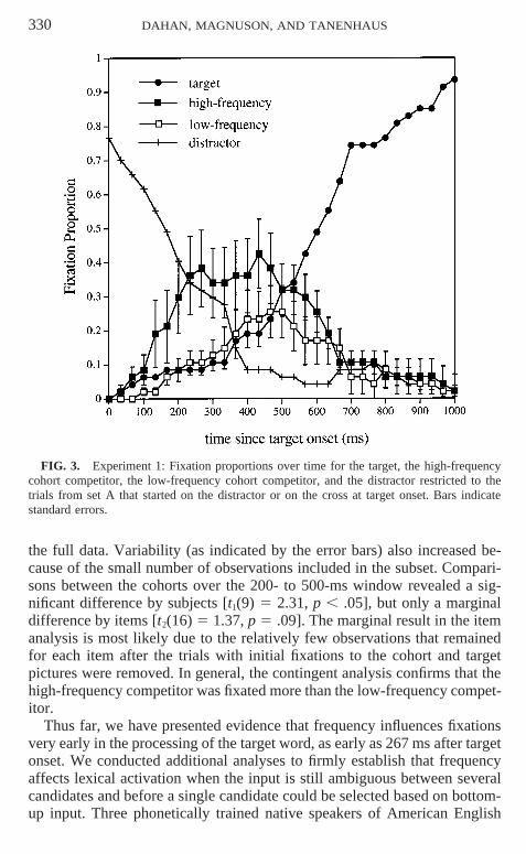
We also conducted a contingent analysis by selecting the trials on whichparticipants were fixating either the distractor or the cross at the onset of thetarget word (47 of the 168 trials, 28%). If participants happened to be lookingat the target or at one of the cohort competitors at the onset of the targetword, they may have kept fixating this picture as the spoken input unfolded,as long as its name was consistent with the spoken input. This analysis en-sures that any advantage observed for fixating the high-frequency cohortover the low-frequency cohort was not influenced by where the subject hap-pened to be fixating at the onset of the target word. Figure 3 presents thefixation proportions for the target, each cohort competitor, and the distractor,from 0 to 1000 ms after target onset, on this subset of the data. As is apparentin the figure, the proportion of fixations to the high-frequency cohort wasgreater than the proportion of fixations to the low-frequency cohort, and themagnitude of the frequency effect was larger for this subset of data than for
330 DAHAN, MAGNUSON, AND TANENHAUS
FIG. 3. Experiment 1: Fixation proportions over time for the target, the high-frequencycohort competitor, the low-frequency cohort competitor, and the distractor restricted to thetrials from set A that started on the distractor or on the cross at target onset. Bars indicatestandard errors.
the full data. Variability (as indicated by the error bars) also increased be-cause of the small number of observations included in the subset. Compari-sons between the cohorts over the 200- to 500-ms window revealed a sig-nificant difference by subjects [t1(9) 5 2.31, p , .05], but only a marginaldifference by items [t2(16) 5 1.37, p 5 .09]. The marginal result in the itemanalysis is most likely due to the relatively few observations that remainedfor each item after the trials with initial fixations to the cohort and targetpictures were removed. In general, the contingent analysis confirms that thehigh-frequency competitor was fixated more than the low-frequency compet-itor.
Thus far, we have presented evidence that frequency influences fixationsvery early in the processing of the target word, as early as 267 ms after targetonset. We conducted additional analyses to firmly establish that frequencyaffects lexical activation when the input is still ambiguous between severalcandidates and before a single candidate could be selected based on bottom-up input. Three phonetically trained native speakers of American English

FREQUENCY AND EYE TRACKING 331
were instructed to determine the point, in the target word, where the signalcould unambiguously distinguish the target from its competitors (e.g., where,in the word /bεnt∫/, they could be certain that bench, and not bed or bell, washeard). Using a speech editor, they selected increasingly larger fragments ofthe target word until they reached a point where the target could be identifiedand the competitors rejected. The names of the targets and competitors wereprovided beforehand. This procedure provided, for each of the 17 items, anestimate of the uniqueness point (with respect to the other alternatives presenton the display). The uniqueness-point estimates were quite similar acrossjudges and correlated highly (mean r 5 .83); they were thus averaged.The mean uniqueness point was 237 ms (ranging from 128 to 352 ms).Uniqueness-point estimates allowed us to test whether frequency effect oc-curred as soon as candidates were activated (i.e., before the uniquenesspoint), as predicted by a frequency mechanism operating very early, or whenonly one candidate matched the signal (i.e., after the uniqueness point), aspredicted by a late response-bias account.
For each of the 17 items, we computed the mean proportion of fixationto the high-frequency and low-frequency competitors over two time win-dows: (1) over the time window extending from the onset of the target wordplus 200 ms to the uniqueness point plus 200 ms—the window where fixa-tions could plausibly be affected by signal information from target onset upuntil the uniqueness point; and (2) over the time window extending fromthe uniqueness point plus 200 ms to the target offset plus 200 ms—the win-dow where fixations could have been influenced from signal informationcoming at or after the uniqueness point. On average, the high-frequency com-petitor was more likely to be fixated than the low-frequency competitor, foreach time window (32% vs 24% for the preuniqueness point window and19% vs 13% for the postuniqueness point window). A two-way (window 3competitor frequency) ANOVA revealed a significant effect of competitorfrequency [F(1, 16) 5 4.7, p , .05] and of window [F(1, 16) 5 29.5, p ,.0001] and no significant interaction (F , 1). This demonstrates that thefrequency effect was not limited to the postuniqueness point window, aspredicted by a late response bias account of frequency, but was already pres-ent in the preuniqueness point time window.
Analysis of Set B Data
In this set, both cohort pictures were presented along with a phonologicallyunrelated target (e.g., the cohort pictures bed and bell were presented alongwith the target mushroom). Fixations to these pictures as the target wordwas heard should have been triggered by the visual characteristics of thepictures only, since their names were phonologically dissimilar to the target.For two participants, a few trials were missing because of technical failures(one for one participant and two for the other participant). Figure 4 presentsthe fixation proportion over time for the target, the high- and low-frequency

332 DAHAN, MAGNUSON, AND TANENHAUS
FIG. 4. Experiment 1: Fixation proportions over time for the target, the high-frequencycohort item, the low-frequency cohort item, and the distractor on the trials from set B. Barsindicate standard errors.
cohort items, and for the distractor. Fixations to both cohort items and tothe distractor steadily decreased while fixations to the target increased as thetarget word was heard. Crucially, in the 200- to 500-ms window, the fixationproportion for the high-frequency cohort item did not surpass that for thelow-frequency cohort item—in fact, the low-frequency cohort item showeda small advantage over its high-frequency counterpart, although the differ-ence was not reliable [t1(9) 5 1.22, p . .10; t2(16) 5 1.19, p . .10). Thus,the analysis of the set B trials indicated that the visual characteristics of thepictures cannot account for the advantage for fixating high-frequency cohortitems observed in set A. The effect can thus be attributed to the influenceof lexical frequency on cohort activation.
Experiment 1 revealed three central results. First, it confirmed that thefixations to targets and competitors are tightly time-locked to the unfoldingacoustic input, as demonstrated in Allopenna et al. (1998). Recall that in ourstudy (as opposed to that of Allopenna et al.), participants had no exposureto the pictures prior to the experiment and quite limited exposure (500 ms)to the four pictures prior to the spoken instruction during each trial. Thus,

FREQUENCY AND EYE TRACKING 333
the time locking is not a consequence of extensive exposure. Second, theresults showed that the probability of fixating a competitor that shares phono-logical similarity with the target word are further influenced by the competi-tor’s lexical frequency in the language. Even though the display limited po-tential responses to four alternatives (i.e., four pictures), an effect of wordfrequency was still observed (at least under conditions where the exposureto the pictures was limited). Finally, the timing of the frequency effect shedslight on the locus of frequency effects in word processing. The fixations tothe high-frequency cohort competitor started diverging from the fixations tothe low-frequency cohort competitor as early as 267 ms after target-wordonset, reflecting fixations that were programmed within the first 100 ms ofthe beginning of the word, and while the input was still ambiguous amongmultiple lexical alternatives (i.e., prior to the uniqueness point). We thus seean effect of word frequency as early as it can be observed. This is incompati-ble with a view of word frequency operating as a late response bias afterlexical access is complete.
Simulations
An important advantage of the eye-tracking paradigm is that hypotheticallexical activations can be mapped onto fixation proportions using an explicit,well-motivated linking hypothesis (Allopenna et al., 1998), allowing forquantitative tests of alternative models. In order to evaluate the various ac-counts of frequency and their fit to our data, we implemented frequency inthe TRACE model (McClelland & Elman, 1986). We chose TRACE becauseit is a well specified and implemented model of spoken-word recognitionand is publicly available. It accounts for a wide variety of phenomena(McClelland & Elman, 1986), including the time course of fixation probabili-ties in tasks like ours (Allopenna et al., 1998). TRACE shares several impor-tant basic properties with other current models of spoken-word recognition.Words are activated incrementally as an input sequence unfolds, proportion-ally to their similarity with the input, and activated words compete for recog-nition.
TRACE is an interactive activation network composed of three levels.Input arrives in the form of idealized, pseudospectral representations of fea-tures over time. The featural nodes have excitatory connections to appro-priate phoneme nodes. Phoneme nodes in turn excite appropriate lexicalnodes. Competition is implemented via lateral inhibitory connections withinthe phoneme and lexical levels. In addition, lexical nodes feed back via excit-atory connections to the phonemes they are connected to. (Feedback connec-tions also exist from phonemes to features, but the weights of these con-nections were set to 0 in McClelland & Elman, 1986, as well as in oursimulations.) Input arrives in featural slices, with phonemes having durationsof 11 slices. Because phonemes are centered 6 slices apart, input slices corre-sponding to a phoneme overlap with slices corresponding to the preceding

334 DAHAN, MAGNUSON, AND TANENHAUS
and following phonemes. Activation spreads forward through the networkfrom feature to phoneme to lexical nodes, after each input slice (with a 1-slice lag for word-to-phoneme feedback).
We compared three different implementations of frequency: frequencyoperating on resting-activation levels, frequency operating on connectionweights, and frequency applied in a postactivation decision rule, as suggestedby Luce and colleagues in the NAM (Goldinger et al., 1989; Luce, 1986;Luce & Pisoni, 1998). In each of these simulations, frequency is viewed asa central component of lexical access; that is, frequency plays a role as soonas lexical candidates become active (this is described in more detail below).The simulations were compared to simulations that did not incorporate fre-quency. These simulations had three goals. The first goal was to determinewhether simulations with frequency would provide a better account for thedata than simulations without frequency. Note that achieving better fits withfrequency as a factor is not trivial because (a) phonological similarity ac-counts for most of the variance and (b) we are not using frequency as a freeparameter; rather, we are using theoretically motivated hypotheses abouthow frequency affects activations to generate activation-driven predictions.The second goal was to use explicit implementations to determine what dif-ferent predictions, if any, competing frequency accounts make about the timecourse of lexical activation. If significant differences arose, the third goalwas to determine which frequency model best fits the data.
We used the publicly available implementation of TRACE.2 We aug-mented the 235-word lexicon included with the distribution with approxima-tions to all of the target and cohort stimuli (but not the distractors) fromExperiments 1 and 2.3 (Distractors were chosen from unrelated items in thelexicon.) We added 51 words for Experiment 1 and 17 words for Experiment2, resulting in a 303-word lexicon.
2 This is available from Jeff Elman at the UCSD Center for Research in Language viaanonymous ftp at ftp://crl.ucsd.edu/pub/neuralnets/. Note that the parameter set included inthis implementation was changed to match those reported by McClelland and Elman (1986)—with the exception of the frequency-scale parameter, which we varied in the simulations re-ported here. These parameters are reported in Appendix B.
3 Because TRACE only incorporates a subset of English segments (the vowels /ɒ, u, i, ö/and the consonants /b, p, d, t, g, k, s, ʃ, ɹ, d, l/), many of our stimuli could only be approxi-mately transcribed. We tried to choose similar segments for substitutions without overusingany segment. We made no attempt to use transcription choices as free parameters. We tran-scribed the words only once and did not tweak our transcriptions to drive the performance ofthe model, with three exceptions: /tö/, /kö/, and /böl/ (original TRACE transcription for toe,cow, and bell, respectively). Because many words contain these syllables, these items did notbecome the most active items given appropriate input. We retranscribed the first two as /töö/and /köö/, which approximates the fact that word-final vowels are lengthened in English, andallowed them to become the most activated words in response to appropriate input. Wechanged the vowel used for bell and bed to /i/ (transcribed as /bil/ and /bid/), which placedthose items in a sparser neighborhood. Our transcriptions are listed in Appendices A and C.

FREQUENCY AND EYE TRACKING 335
Frequency in resting levels. The approach usually taken in interactive acti-vation models is to make resting levels proportional to frequency (McClel-land & Rumelhart, 1981). On this approach, each unit has a functional biasassociated with it, such that high-frequency items have a head start in theform of higher activation in the absence of bottom-up input and their activa-tions decay slightly more slowly. The TRACE implementation includes amethod for incorporating frequency, but so far as we know, this aspect ofthe model has not been explored previously. In all the published reports weare aware of, frequency was turned off by setting the frequency-scale param-eter to zero. However, a nonzero frequency value can be specified for eachlexical item, which affects its resting-activation level. Resting level is deter-mined by Eq. (1) as follows:
ri 5 R 1 s[log10(c 1 fi)] 1 pi, (1)
where ri is the resting activation for unit i, R is the default resting activation,s is the frequency-scaling constant; fi is the frequency of item i (number ofoccurrences per million words reported by Francis & Kucera, 1982; itemsnot included in that corpus were given frequencies of 1), c is a constant thatprevents taking the log of 0 or 1 and can also decrease the initial slope ofthe log transform (we set c to 1.0 for this method, so there was little ef-fect on the slope), and pi is a top-down factor (intended, for instance, forsemantic-priming simulations) which was set to 0 for all our simulations.
Our initial explorations of this frequency implementation revealed twomain constraints. First, if resting values are greater than 0, the activationsof lower frequency items will be driven toward the minimum possible activa-tion value by higher frequency nodes, even in the absence of bottom-upinformation. This is because units with positive activation can inhibit otherunits within the same layer. Therefore, in order for frequency biases to havea stable effect, even items with the highest frequencies must not have restinglevels greater than 0. This means that the default resting level R has to beset sufficiently low that the frequency-scaling constant s can be set highenough to achieve a wide range of resting levels less than 0. We did twothings to accomplish this. First, we set a ceiling for frequency values: Itemswith a frequency greater than 1000 were treated as having a frequency of1000 (only eight items in the TRACE lexicon were affected, none of whichwere among our stimuli). Second, we set the default resting level R to 20.3.(We changed the TRACE implementation to report activations less than 0;note that our results could not be replicated without making this change.)This combination allowed a maximum value of 0.1 for the frequency-scalingconstant s, which would give the highest frequency items resting levels of0. We determined that a value of .06 gave the best balance of fits to the datafrom Experiments 1 and 2 with this method.

336 DAHAN, MAGNUSON, AND TANENHAUS
We converted activations to response probabilities using the Luce choicerule (R. D. Luce, 1959).4 Activations, a, are converted to response strengths,S, as shown in Eq. (2), where k is a constant that determines the amount ofseparation between strengths. We set k to 7 for all of the simulations wereport, as this was the fixed value that Allopenna et al. (1998) used to fitsimilar data. The exponential transformation in Eq. (2) ensures that no valuesare negative and amplifies large activation values. Response probabilities foreach item, P(Ri), are simply normalized response strengths, as shown in Eq.(3) as follows:
Si 5 ekai (2)
P(Ri) 5Si
^n
j51
Sj.
(3)
Note that the conversion to response probabilities embodies a simple as-sumption about the role of visual information in our task. Activations aregenerated in a bottom-up fashion on the basis of phonetic input. All lexicalitems enter into the activation and competition process. However, since onlyfour responses are possible given the visual display, only the four displayeditems enter into the decision rule. We refer to this method as RDLREST becauseit uses the R. D. Luce choice rule to evaluate activations with frequencyinstantiated in resting levels. We refer to simulations without frequency asthe RDLNO FRQ method.
Allopenna et al. (1998) used an additional step that scaled response proba-bilities to be proportional to the total amount of activation among the four
4 Determining activations from TRACE is not a trivial process. Word units in TRACE func-tion as templates. For a word unit to become highly active, it must be well aligned withphonemic (and featural) inputs. TRACE avoids the alignment problem by aligning a copy ofeach word unit every three input slices. Given input, TRACE reports the activity of copiesof each word unit aligned at different slices. The experimenter must decide how to decodethe word-unit patterns of activation. The method we used was to determine which copy of aword unit reached the highest activation and then use the activation of that unit over all inputcycles as the activation of that word. We assume McClelland and Elman (1986) used a similarmethod when they examined activations for their simulations. They reported activations orresponse probabilities based on units aligned with a particular slice of the input, although theydid not explicitly discuss how they chose that slice (see Frauenfelder & Peeters, 1998, for thedescription of a similar method). This procedure is problematic because it cannot be imple-mented in an incremental fashion; it requires an omniscient observer to compare peak activa-tions after processing is finished. Incremental methods are possible. Each lexical item couldhave an associated decision node that would either summate the responses of all copies ofthe word template at all slices or report the activation of the most active word template ateach slice. For the purposes of the current article, we use the simple method we have describedand leave this issue open for future research.

FREQUENCY AND EYE TRACKING 337
possible visible targets at each time slice. This was necessary because inthe Luce choice rule, given equivalent activations, the minimum responseprobability for any item is 1/n, where n is the number of possible responses.Allopenna et al. instructed participants to fixate a central fixation cross imme-diately before the critical instruction was heard, with the result that the fixa-tion proportions at the onset of target words were almost always 0 for allobjects (since participants were fixating the central cross). For the currentexperiment, we did not give participants any explicit instructions regardingfixations. Participants were thus about equally likely to be fixating any pic-ture in the display at the onset of target words. Thus, the basic choice rule,which assigns response probabilities of 1/n in the absence of bottom-up in-put, maps perfectly onto our task.
Frequency in connection weights. Another way to incorporate frequencyin interactive activation models, advocated by MacKay (1982, 1987), is tomake the weights (or connection strengths) associated with lexical units pro-portional to their frequency. Although implementations of frequency in rest-ing levels or in connection weights are very similar to each other (e.g., Dell,1990), our simulations show that the two implementations differ in one cru-cial respect. In order to implement frequency in the connection weights, wescaled phoneme-to-word input according to lexical frequency according toEq. (4) as follows:
a′pi 5 api[1 1 (apis[log10(c 1 fi)])], (4)
where api is the activation to lexical unit i from phoneme p. We found thata value of .13 for s achieved the best balance of fits for the data from Experi-ments 1 and 2, and c was set to 1.0. Note that with frequency implementedin connection weights, the scaling factor s is not constrained in the sameway as for frequency implemented in resting levels, since units remain atthe same default resting level until they receive bottom-up input. Activationswere converted to response probabilities using the Luce choice rule as in theresting-level method. We refer to this method as RDLWT.
Frequency in the decision rule. The final method used to incorporate fre-quency was based on the principles of the NAM. In this model, units corre-sponding to acoustic-phonetic patterns are activated on the basis of bottom-up input. These pattern units connect to decision units, which correspond todifferent lexical items. Decision units compute the Stimulus Word Probabil-ity (SWP) for their corresponding lexical item on the basis of the bottom-up pattern input (that is, the probability that the lexical item is being heardgiven the current input). They also have access to higher level lexical infor-mation, such as word frequency, and have access to the summed SWPs forall other lexical items. Based on these input sources, decision units computethe probability of identifying their corresponding word according to Eq. (5)as follows:

338 DAHAN, MAGNUSON, AND TANENHAUS
P(ID) 5SWPi fi
^n
j51
SWPj fj,
(5)
where i is the lexical item corresponding to the decision unit, fi its frequency,and the denominator is the summed frequency-weighted SWPs for all items,including i.5 Note the similarity between Eqs. (3) and (5); Eq. (5) would bea frequency-weighted variant of the R. D. Luce (1959) choice rule if TRACEresponse strengths were used as SWP estimates. While Luce (1986) and Luceand Pisoni (1998) used segmental confusion matrices to estimate SWPs, theyalso suggested that a TRACE-like interactive activation system could formthe front-end to the NAM, such that SWPs would correspond to activations.A key difference in such an implementation compared to the standardTRACE model is the locus of frequency effects. When frequency is incorpo-rated into the activation component of an interactive activation model likeTRACE, its effects percolate throughout the system. In contrast, if frequencyonly comes into play at a postactivation decision stage, its effects will beconfined to this decision stage, and Goldinger et al. (1989) predicted thatthese two implementations ought to have very different results. The ramifi-cations of the two implementations are complex enough that simulations arecalled for to test in what ways they are different. In order to implement adecision rule that incorporates frequency independently of activations, wesimply used TRACE activations (without frequency) as estimates of SWPs.This is equivalent to frequency-weighting response strengths, as in Eq. (6)as follows:
Si 5 SWPi 5 ekai [log10(c 1 fi)], (6)
where ai is the activation of the lexical unit for word i, fi is its frequency,and c is a constant. Unlike the other simulation methods, we found that fitswere substantially improved by manipulating the parameter c. A value of15 was used for c for both experiments (making c larger improves the fitfor Experiment 2, but decreases the fit for Experiment 1). Alternatively, onecould use a frequency scaling parameter to control the influence of frequencyin Eq. (6). However, scaling f by values greater than 1 has similar effectsas increasing c, and values less than 1 have the undesirable effect of makingthe log-transform more linear. Response strengths were converted to re-sponse probabilities using Eq. (3). We refer to this simulation method as the
5 Note that Luce and his colleagues usually separate the SWP of item i from the SWPs ofthe phonological neighbors of this item, which they denote as NWPs (neighbor-word probabili-ties). Without an a priori way of dividing the lexicon into neighbors and nonneighbors, it issimpler to refer to the SWPs of every word given the current input (most will approach 0).

FREQUENCY AND EYE TRACKING 339
RDLPOST method because it is the Luce choice rule with frequency appliedat the ‘‘postactivation’’ stage.
Note that this implementation is somewhat inconsistent with the way theNAM has been described by Luce and colleagues. According to Goldingeret al. (1989), in the NAM, ‘‘the effects of frequency are not realized untilthe selection phase of the recognition process [. . .] frequency is assumedto exert its influences after initial activation but before lexical access occurs’’(p. 504). Thus, frequency should not come into play during the initial pro-cessing, whereas in our implementation, frequency comes into play immedi-ately, given nonzero activation. We did not implement a staged applicationof frequency of this sort. However, we can infer from the results of theRDLNO FRQ (without frequency) and RDLPOST simulations what the results ofsuch an implementation would be: Early on, a system with a late-actingfrequency mechanism would resemble TRACE without frequency, i.e.,RDLNO FRQ. Once some sort of threshold were reached (e.g., one or moreitems crossed an activation threshold), frequency would come into play, andthe results would resemble RDLPOST from that point onward.
Simulation results. We conducted our simulations by presenting each tar-get word to TRACE, one at a time. All lexical items were allowed to com-pete. Figure 5 shows the raw TRACE activations averaged over all the stimu-lus items. In the top panel, activations are shown with no frequency influence(activation for the high-frequency and the low-frequency competitors arethus identical); in the middle panel, frequency is incorporated into restingactivations; and in the bottom panel, frequency is incorporated into connec-tion weights.6
We then computed response probabilities for each of the four methods(RDLNO FRQ, RDLREST, RDLWT, and RDLPOST). A crucial issue was how to mapcycles onto real time. We used stimulus length to equate simulation timeand real time. Our stimuli for Experiment 1 had a mean duration of 498 ms.Our stimuli, as represented in TRACE, had a mean duration of 40.1 cycles.If we equate stimulus time between our natural speech and TRACE represen-tations, each cycle would be equivalent to 12.4 ms. Given that we sampledeye movements at 30 Hz (i.e., every 33.33 ms), we aligned cycles to millisec-onds by linearly interpolating 11 intermediate steps between cycles (makingeach new cycle equivalent to 1.03 ms) and then downsampling to every 32ndpoint. Thus, each downsampled cycle corresponded to 33.12 ms. Allopennaet al. (1998) were able to equate 1 cycle to 11 ms, and, therefore, 3 cyclesto one video frame, because their talker had a slightly faster speech rate.Note that it is quite remarkable that the temporal dynamics of TRACE allowsuch a principled method for equating simulation time and real time.
6 Activations vary from 2100 to 100 because TRACE multiplies the output values by 100.Before computing response probabilities, we multiplied the activations by .01 to convert themback to a scale varying from 21 to 1.

340 DAHAN, MAGNUSON, AND TANENHAUS
FIG. 5. Experiment 1 simulations: TRACE activations over time for the target, the high-and low-frequency competitors, and the distractor when frequency is turned off (top), whenfrequency is coded in resting activations (middle), and when frequency is coded in connectionweights (bottom).

FREQUENCY AND EYE TRACKING 341
Another important issue is how to align simulation points and data points.Allopenna et al. (1998) added six extra frames of no activation to the begin-nings of their simulations, which they equated with the time it takes to planand launch an eye movement. We found that our various simulation meth-ods required slightly different alignments for optimal fits to the data, so wetreated alignment as a free variable (two extra frames of no activation wereadded for RDLPOST, three for RDLREST and RDLNO FRQ, and four for RDLWT;however, this only gave an average improvement of .07 in r2 compared todirect alignment).
In Fig. 6, activations have been transformed into response probabilitiesfor each of the four simulation methods (RDLNO FRQ, RDLREST, RDLWT, andRDLPOST).
Table 1 shows the root mean squared (RMS) error between the data andsimulation methods computed over two different windows: all data pointsfrom 0 to 1000 ms and from 200 to 500 ms (the region where reliable cohorteffects were observed in the data). RMS error gives a measure of the absolutefit. The means for each item are shown to help interpret the RMS values.(Since RMS is an absolute measure, an RMS of 0.1 could be quite good fordata with a mean near 1.0, but could be quite poor for data with a mean near0.) Table 2 shows the corresponding r2 values. In addition, RMS and r2 val-ues computed on the difference between high- and low-frequency cohortsare reported in each table. We included this measure because all of the meth-ods yielded relatively small RMS and large r2 values, suggesting a good fitwith the data. For RMS, this was because the frequency-based differenceswe observed were relatively subtle (even the no-frequency method yieldedRMS values comparable to the other methods for the high- and low-fre-quency items). For r2, this was because the differences from time step totime step are important. To achieve a high r2 value, the simulated data pointsmust show decreases and increases proportional to those found in the data.Taking a difference score allows us to make a stronger test: Do the simulateddata points also capture the differences between high- and low-frequencycompetitors? We thus concentrate on these values when comparing the dif-ferent simulations.
As is apparent in Tables 1 and 2, the RDLNO FRQ method did not fit thedata as well as the other methods, especially in terms of the difference be-tween high- and low-frequency competitors in the 200- to 500-ms region.The RMS is about twice as great as that for the other methods, and thisimplementation provides no correlation with the data over time. All the othermethods fit the data well. The differences in fixation probabilities betweenthe high- and low-frequency competitors are shown in Fig. 7. As can beseen in the figure, all three methods incorporating frequency provide similarpredictions. The main difference is in the initial difference predicted by theRDLWT method. With this method, frequency effects are proportional to acti-vation in the system. Prior to substantial bottom-up input, no frequency dif-

342 DAHAN, MAGNUSON, AND TANENHAUS
FIG. 6. Experiment 1 simulations: Fixation probabilities over time for the target, the high-and low-frequency competitors, and the distractor for each of the four frequency implementa-tions (see text).
ference is predicted. As more input arrives, the frequency difference gradu-ally increases. The other two frequency methods, RDLREST and RDLPOST,predict a frequency bias, even with little bottom-up activation. Thus, theRDLWT method is able to capture one significant feature of the data that theothers cannot: a frequency effect with a gradual onset, modulated by bottom-up activity. It is in this respect that the resting-level and connection-strength

FREQUENCY AND EYE TRACKING 343
TABLE 1RMS Measures of Model Fits to Experiment 1 for the Target, the High-Frequency (HF)
and the Low-Frequency (LF) Cohort Competitors, and the Distractor, on the 0- to 1000-ms(All) and the 200- to 500-ms (Section) Windows
Mean Item RDLNO FRQ RDLREST RDLWT RDLPOST
.514 Target (All) .117 .093 .090 .103
.278 Target (Section) .081 .038 .075 .043
.182 HF Cohort (All) .044 .053 .027 .055
.310 HF Cohort (Section) .037 .040 .022 .048
.148 LF Cohort (All) .038 .033 .031 .033
.232 LF Cohort (Section) .053 .031 .029 .028
.125 Distractor (All) .070 .076 .062 .076
.135 Distractor (Section) .069 .072 .057 .074
.049 HF–LF (All) .056 .069 .037 .069
.080 HF–LF (Section) .086 .044 .029 .048
Note. Means for the data are shown in the leftmost column to guide interpretation of theRMS values.
implementations are not simple variants of each other; only the connection-weight implementation gives rise to a gradual (although still immediate andfast) onset of frequency.
All of the implementations that we have evaluated thus far assume thatfrequency applies early in the recognition process. However, one might de-fend a model in which frequency comes into play when the system is prepar-ing to generate a response, that is, after lexical access and prior to generatingan eye movement. This would be consistent with the late-acting responsebias argued for by Connine et al. (1993). The argument would be that evenwhen activation levels are low, there is still a small probability that activation
TABLE 2r2 Measures of Model Fits to Experiment 1 for the Target, the High-Frequency (HF) andthe Low-Frequency (LF) Cohort Competitors, and the Distractor, on the 0- to 1000-ms
(All) and the 200- to 500-ms (Section) Windows
Item RDLNO FRQ RDLREST RDLWT RDLPOST
Target (All) .955 .969 .965 .969Target (Section) .969 .963 .969 .968HF Cohort (All) .909 .931 .961 .931HF Cohort (Section) .606 .590 .638 .631LF Cohort (All) .942 .923 .940 .923LF Cohort (Section) .263 .091 .759 .090Distractor (All) .754 .761 .795 .756Distractor (Section) .672 .652 .691 .667HF–LF (All) .015 .106 .491 .139HF–LF (Section) .008 .342 .550 .475

344 DAHAN, MAGNUSON, AND TANENHAUS
FIG. 7. Experiment 1 simulations: Fixation-probability differences between the high- andthe low-frequency competitors over time for the data and each of the four frequency implemen-tations (see text).
of a lexical alternative will cross a response threshold. Frequency would thenoperate as a constant bias and apply to lexical candidates that cross threshold.The RDLPOST method could be easily adapted to do something like this, e.g.,by only allowing frequency to weight response strengths after a certain num-ber of cycles of processing or when activations surpass a threshold. Theresult would resemble pasting the RDLNO FRQ and RDLPOST results together:Prior to the point at which frequency applied, this ‘‘late’’ method wouldlook exactly like the RDLNO FRQ method. From the point at which frequencyapplied, it would look exactly like RDLPOST, with a sudden jump betweenthe two patterns. However, there is no motivation to implement such a mech-anism. Because frequency has a gradual and early onset in our data, thereis no basis to prefer a late-acting, sudden-onset frequency bias. Moreover,modifying the postaccess model to assume that lexical access can take placeas early as would be necessary to accommodate our data would clearly vio-late the spirit of the postaccess hypothesis: The threshold for generating aresponse after lexical access would have to be so low as to be indistinguish-able from a model without a threshold.

FREQUENCY AND EYE TRACKING 345
Summary and Conclusions
Experiment 1 demonstrated that fixations to objects in the visual set thatshare phonological similarity with the sound pattern of the target word areaffected by the frequency with which the names of the objects occur in thelanguage. When both high-frequency and low-frequency cohort competitorswere present, participants were more likely to fixate the high-frequency com-petitor than the low-frequency competitor. Furthermore, the difference infixations between high- and low-frequency competitors was observed veryearly, when the acoustic signal was still lexically ambiguous. The results areconsistent with predictions from models in which frequency affects lexicalaccess as soon as lexical items are activated by bottom-up input. The TRACEmodel accounted for a large proportion of the variance in the time courseof fixation probabilities, regardless of whether frequency was implementedin resting activation levels, connections weights, or as a bias applied continu-ously to (but independently of ) activations (although the connection weightmethod yielded the best quantitative and qualitative fits).
EXPERIMENT 2
Experiment 2 was conducted to determine whether it was possible to ob-serve an effect of target frequency when none of the other pictures had namesthat were phonologically related to the name of the referent. Demonstratinga frequency effect on target fixations, with no competitor pictures with namesphonologically similar to the target’s in the display, is important because itwould provide a replication of the frequency effect using a different measureand would allow us to further evaluate the mechanism by which frequencyoperates during lexical processing. Moreover, finding such an effect on targetfixations would be inconsistent with the possibility that participants adopt averification strategy (i.e., naming the visually present objects prior to thespoken instruction and then matching the sound pattern of the target wordwith the preactivated names). This verification strategy could account forthe frequency difference on fixations to cohort competitors in Experiment 1by assuming that frequency biases the storage and/or retrieval of the preacti-vated names. However, because no frequency effect was found on fixationsto the competitors in the set B data (when the target name did not overlapwith the cohorts’ names), one would also have to assume that the frequencybias in the verification strategy only applies to names that match the tar-get word. In Experiment 2, a referent picture was presented along withthree pictures with phonologically unrelated names. The name of the referentwas either low-frequency or high-frequency. Assuming that high-frequencywords are activated faster than low-frequency words, and that fixations areinfluenced by lexical activations, we predicted that participants would fixatethe high-frequency referent picture (before clicking on it with the mouse)

346 DAHAN, MAGNUSON, AND TANENHAUS
faster than the low-frequency referent picture. A verification strategy wouldnot predict such a difference; both high-frequency and low-frequency refer-ent pictures should be fixated equally fast because in both conditions, thetarget picture is the only visually present picture whose name matches thetarget word.
Method
Participants
Eighteen students at the University of Rochester participated in this experiment and werepaid $7.50. None of them had participated in Experiment 1.
Materials
The materials consisted of 21 pairs of phonologically similar words which differed in lexicalfrequency according to the Francis and Kucera (1982) counts (e.g., bell has a frequency of23 per million and bed a frequency of 139 per million). We were unable to find pairs of wordsfor which one item was very low in frequency and the other very high. However, we madesure that there was a large frequency difference between each item of the pair. The meanfrequency of the high- and low-frequency items was 104.0 per million and 14.4 per million,respectively. Each pair was associated with three phonologically unrelated distractors (e.g.,sock, headphones, and knife). The complete set of materials is presented in Appendix C. Ona given trial, either the low-frequency or the high-frequency item was presented along with itsthree distractors. In addition to the 21 pairs and their distractors, 16 sets of four phonologicallyunrelated items were constructed to serve as filler trials. Two lists were constructed by varyingwhether the high-frequency or the low-frequency item of each pair was the target. Nine partici-pants were randomly assigned to each list. For each list, three random orders were created;approximately the same number of participants were assigned to each order.
The 169 [(21 3 5) 1 (16 3 4)] pictures were selected from the Snodgrass and Vanderwart(1980) and the Cycowicz, Friedman, Rothstein, and Snodgrass (1997) picture sets as well asfrom children’s picture dictionaries and a commercially available clip-art database; all wereblack-and-white line drawings.
Before we could conclude that a frequency effect on target fixations was specifically causedby differences in lexical frequency between the two sets of words, we needed to rule out thepossibility that a frequency effect might result from differences in object-recognition perfor-mances or in name agreement. For instance, people might fixate the pictures associated withlow-frequency names more slowly than pictures associated with high-frequency names be-cause the pictured representations of the low-frequency items were harder to recognize orbecause the words used to refer to the pictures with low-frequency names were less commonlyassociated with these pictures than were the words and the pictures with high-frequency names.Therefore, we conducted two control experiments. In the first experiment, participants madea speeded semantic categorization on the pictured objects that did not require them to generateitem names (i.e., is the pictured object natural or artifact). In the second experiment, theygenerated a name. The details of these experiments are presented in Appendix D. The resultsshowed no evidence that the pictures of the high-frequency items were recognized more rapidlyor named more accurately than the pictures of the low-frequency items. (In fact, the picture-recognition experiment revealed a small bias in favor of the low-frequency item pictures.)Thus, faster fixations to the pictures with higher frequency names could not be attributed tocharacteristics of the pictures.
The spoken instructions were recorded by a female native speaker of English in a soundproofroom, sampling at 22,050 Hz. The average duration of the target word was 625 ms for thehigh-frequency items and 632 ms for the low-frequency items.

FREQUENCY AND EYE TRACKING 347
Procedure
As in Experiment 1, participants were seated at a comfortable distance with the computerscreen, and their eye movements were monitored as they followed the spoken instructions.The structure of each trial was as follows: First, a 5 3 5 grid with a centered cross appearedon the screen, and participants were instructed to look at the cross and to click on it. Thenfour line drawings and four colored geometric shapes appeared on specific cells of the grid.Immediately after the pictures appeared, the spoken instruction started. Because we wantedto analyze the time it took participants to direct their attention to and fixate the target picture,we attempted to minimize the probability for participants to be already fixating the targetpicture at target onset. The instruction was thus composed of two parts. First, participantswere asked to point to one of the distractor pictures using the computer mouse (e.g., ‘‘Pointto the sock’’). After a delay of 300 ms to allow participants to move the mouse cursor to thedistractor picture, they were instructed to point to the target picture (e.g., ‘‘now the bed’’).Then they were asked to move the target picture above or below one of the geometric shapes(e.g., ‘‘Click on it and put it above the circle’’). Once this was accomplished, the next trialbegan. By asking participants to point to one of the distractor pictures immediately beforepointing to the target picture, we minimized the proportions of trials where subjects werefixating the target picture at the onset of the target word. On 14 of the 16 filler trials, subjectswere instructed to click on and move the first picture they pointed to (e.g., ‘‘Point to theballoon. Click on it, and put it below the square’’). This was intended to ensure that peopledirected their attention to the first picture. The positions of the geometric shapes were fixedfrom one trial to the other. The position of each picture was randomized for each subject andeach trial.
Results and Discussion
The coding procedure was identical to that described for Experiment 1.Fixations were coded from the onset of the target word until participantsfixated the target picture and initiated a mouse movement to point to it. Onetrial was discarded because the participant pointed to the picture withoutfixating it. Overall, people made 2.14 fixations on average before reachingthe target picture, 2.13 fixations when the target was high-frequency, and2.14 fixations when the target was low-frequency. For 6 trials (1.6% of thedata), participants were already fixating the target picture at the onset of thetarget word; these trials were removed from the subsequent analyses. Thedelays between the onset of the target and the onset of the last fixation,always to the target, were analyzed after excluding the trials where this delaywas less than 200 ms or greater than or equal to 1300 ms. Fixations occurringbefore 200 ms were assumed to have been programmed before the onset ofthe target word; trials where participants took more than 1300 ms to fixatethe target were treated as outliers. In total, 19 trials (5% of the data) wereexcluded (12 with low-frequency targets and 7 with high-frequency targets).
On average, the pictures corresponding to high-frequency items werefixated faster than those corresponding to low-frequency items (563 ms vs625 ms). Planned comparisons revealed that this difference was reliable[t1(17) 5 3.26, p , .005; t2(20) 5 1.99, p , .05]. The proportions of fixationsto the high-frequency and low-frequency targets over time are shown in Fig.

348 DAHAN, MAGNUSON, AND TANENHAUS
FIG. 8. Experiment 2: Fixation proportions over time for the high-frequency and low-frequency targets. Bars indicate standard errors.
8. At 400 ms after target onset, the proportion of fixations to the high-frequency target surpassed the proportion of fixations to the low-frequencytarget, indicating that participants fixated the high-frequency target earlierthan the low-frequency target. Again, this result reveals the influence of fre-quency very early in the word-recognition process, given the delay to pro-gram and launch an eye movement. The fixation analysis confirms what theanalysis on latencies showed: The pictures associated with high-frequencyitems were fixated faster than the pictures associated with low-frequencyitems. This result is difficult to reconcile with an account that participantsin our experiments adopted a special verification strategy based on fre-quency. We discuss the implications of this result for the eye-tracking para-digm in more detail under General Discussion. We also discuss additionalempirical evidence that demonstrates that word recognition in the eye-tracking paradigm does not bypass normal lexical processing.
Simulations
The same procedures were used in the present simulations as were usedfor Experiment 1. However, for each pair of high- and low-frequency targets,

FREQUENCY AND EYE TRACKING 349
each target word was presented as a separate input to TRACE. Three dis-tractors with similar frequencies to those for the distractors used in the exper-iment were chosen from the TRACE lexicon. The same three distractors wereused for both members of each pair. Figure 9 presents the overall activationpatterns. In the top panel, average high- and low-frequency target activationsare shown when frequency was not used. The middle panel shows the corre-sponding averages observed when frequency was incorporated in resting ac-tivations (frequency scaling constant s 5 .06), and the bottom panel showsthe results when frequency was incorporated in phoneme-to-word connectionstrengths (frequency scaling constant s 5 .13). Note that there was a slightadvantage for high-frequency items when frequency was not included. Thiswas due to differences in neighborhoods among the items. However, theadditional difference due to the effect of frequency was clearly substantial.
In contrast to Experiment 1, the task used in Experiment 2 was similar tothat used by Allopenna et al. (1998). While Allopenna et al. used explicitfixation instructions to ensure that subjects fixated a single location at targetonset, we devised task constraints that made it likely that subjects would notbe fixating the target picture at the onset of the target word (i.e., by askingthem to point to a distractor picture before the critical instruction). Therefore,for Experiment 2, an additional method for computing response probabilitieswas included: the scaled Luce choice rule used by Allopenna et al. As dis-cussed above, the simple form of the Luce choice rule predicts that for equiv-alent response strengths (even when all are 0), the minimum response prob-ability is 1/n, where n is the number of possible responses. In order toapproximate a context in which task constraints dictate nonuniform probabil-ities for all responses (e.g., when subjects are instructed to fixate a particularitem or to make a visually guided movement to an object other than thetarget prior to the critical instruction), Allopenna et al. scaled activations asa function of activation in the current time slice relative to the maximumactivation observed during processing, using the scaling factor shown in Eq.(7), where max(at) is the maximum activation in time slice t, and max(a) isthe maximum activation observed during all time steps:
∆ 5max(at)max(a)
. (7)
We incorporated this into our choice rule simply by multiplying responsestrengths by the scaling factor prior to computing response probabilities. Werefer to response probabilities computed with this method as AMTNO FRQ (Al-lopenna et al. method, no frequency), AMTREST (activations with frequencyinstantiated in resting levels), and AMTWT (activations with frequency in-stantiated in connection weights).
In order to compute scaled response probabilities with frequency instanti-

350 DAHAN, MAGNUSON, AND TANENHAUS
FIG. 9. Experiment 2 simulations: TRACE activations over time for the high- and low-frequency targets when frequency is turned off (top), when frequency is coded in restingactivations (middle), and when frequency is coded in connection weights (bottom).

FREQUENCY AND EYE TRACKING 351
ated at a ‘‘postactivation’’ stage (AMTPOST), we needed a different scalingfactor than the one described in Eq. (7). This is because the scaling factorin Eq. (7) is based on activations; in the decision-rule method, raw activationsdo not incorporate frequency. In order to incorporate frequency in the scalingwithout directly applying it on activations, we devised the method presentedin Eq. (8):
∆ 5max(at 1 f 4)max(a 1 f 4)
, (8)
where at is the maximum activation (without frequency) at time t; a themaximum activation observed during all time steps; and f the item’s log-transformed frequency [see Eq. (6)] raised to the fourth power (to amplifythe frequency effect).
Figure 10 presents the human data for the high- and low-frequency targets,as well as response probabilities calculated using the four different methodsused for Experiment 1 (RDLNO FRQ, RDLREST, RDLWT, and RDLPOST). In Figure11, we present the data with the AMT methods computed using activationswithout frequency (AMTNO FRQ), with frequency in resting levels (AMTREST),in connection weights (AMTWT), or in a scaled decision rule (AMTPOST). Fig-ure 12 superimposes the differences between high-frequency and low-frequency targets from the data and the four RDL and AMT variants.
Tables 3 and 4 present RMS and r2 values for the high- and low-frequencytargets and for the difference between the two for two windows of interest:a window including all data points from 0 to 1000 ms and a window includeddata points from 200 to 1000 ms, since the frequency difference manifestsitself from about 200 ms onward.
The fit measures confirm the impression given by Fig. 12. As for Experi-ment 1, the RDLWT method is superior to RDLREST and RDLPOST, and the AMTmethods, by explicitly incorporating task constraints, provide the best fit tothe data. The three AMT methods that incorporate frequency (AMTREST,AMTWT, and AMTPOST) provide roughly comparable fits as measured by RMSand r2 values for the high-frequency/low-frequency difference for both win-dow analyses. AMTPOST provides high r2 values, but its RMS is 30% higherthan those for the other two AMT variants. This is because the scaling factorin Eq. (8) only partially succeeds in reducing initial activation values. Mostof the improvement in fit compared to RDLPOST is due to sustaining the high-frequency/low-frequency difference. Thus, a substantial contribution towardfitting this data comes from choice rules that explicitly incorporate the taskconstraints faced by the subject.
These simulations replicate the main result of the simulations of Experi-ment 1 using the same set of parameters. Response probabilities computedfrom TRACE activations account for substantial amounts of variance in our

352 DAHAN, MAGNUSON, AND TANENHAUS
FIG. 10. Experiment 2 simulations: Fixation probabilities over time for the target, thehigh- and low-frequency competitors, and the distractor, for the data and each of the fourRDL frequency implementations (see text).
time-course data, and the different methods of implementing frequency donot differ greatly. The importance of this result will be discussed under Gen-eral Discussion. The simulations of the data from Experiment 2 emphasizethe importance of representing task constraints in simulations. The AMTmethods, which approximate the task constraints of Experiment 2, providebetter fits than the RDL methods.

FREQUENCY AND EYE TRACKING 353
FIG. 11. Experiment 2 simulations: Fixation probabilities over time for the target, thehigh- and low-frequency competitors, and the distractor for the data and each of the four AMTfrequency implementations (see text).
GENERAL DISCUSSION
Two experiments used eye movements to investigate the time course offrequency effects during spoken-word recognition in continuous speech us-ing a task in which subjects followed spoken instructions to click on andmove pictures in a display. In Experiment 1, a target picture was presented

354 DAHAN, MAGNUSON, AND TANENHAUS
FIG. 12. Experiment 2 simulations: Fixation-probability differences between the high-and the low-frequency competitors over time for the data and each of the four RDL frequencyimplementations (top) and the data and each of the four AMT frequency implementations(bottom).

FREQUENCY AND EYE TRACKING 355
TA
BL
E3
RM
SM
easu
res
ofM
odel
Fits
toE
xper
imen
t2
for
the
Tar
get,
the
Hig
h-Fr
eque
ncy
(HF)
and
the
Low
-Fre
quen
cy(L
F)C
ohor
tC
ompe
titor
s,an
dth
eD
istr
acto
ron
the
0-to
1000
-ms
(All)
and
the
200-
to10
00-m
s(S
ectio
n)W
indo
ws
Mea
nIt
emR
DL
NO
FRQ
RD
LR
EST
RD
LW
TR
DL
POST
AM
TN
OFR
QA
MT
RE
STA
MT
WT
AM
TPO
ST
.492
HF
Tar
get
(All)
.092
.141
.105
.145
.092
.084
.104
.086
.592
HF
Tar
get
(Sec
tion)
.062
.106
.080
.093
.096
.085
.109
.058
.440
LF
Tar
get
(All)
.121
.140
.128
.149
.102
.082
.095
.066
.527
LF
Tar
get
(Sec
tion)
.078
.130
.113
.111
.108
.083
.099
.048
.054
HF
–LF
(All)
.063
.051
.042
.049
.064
.022
.024
.036
.065
HF
–LF
(Sec
tion)
.070
.048
.047
.045
.072
.025
.027
.034
Not
e.M
eans
for
the
data
are
show
nin
the
left
mos
tco
lum
nto
guid
ein
terp
reta
tion
ofth
eR
MS
valu
es.
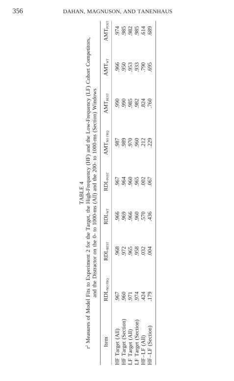
356 DAHAN, MAGNUSON, AND TANENHAUS
TA
BL
E4
r2M
easu
res
ofM
odel
Fits
toE
xper
imen
t2
for
the
Tar
get,
the
Hig
h-Fr
eque
ncy
(HF)
and
the
Low
-Fre
quen
cy(L
F)C
ohor
tC
ompe
titor
s,an
dth
eD
istr
acto
ron
the
0-to
1000
-ms
(All)
and
the
200-
to10
00-m
s(S
ectio
n)W
indo
ws
Item
RD
LN
OFR
QR
DL
RE
STR
DL
WT
RD
LPO
STA
MT
NO
FRQ
AM
TR
EST
AM
TW
TA
MT
POST
HF
Tar
get
(All)
.967
.968
.966
.967
.987
.990
.966
.974
HF
Tar
get
(Sec
tion)
.960
.972
.969
.964
.989
.990
.950
.985
LF
Tar
get
(All)
.971
.965
.966
.960
.970
.985
.953
.982
LF
Tar
get
(Sec
tion)
.974
.958
.960
.965
.960
.982
.933
.985
HF
–LF
(All)
.424
.032
.570
.002
.212
.824
.790
.614
HF
–LF
(Sec
tion)
.179
.004
.436
.067
.229
.760
.695
.689

FREQUENCY AND EYE TRACKING 357
along with two pictures associated with cohort competitors and a distractorpicture. The cohort competitors differed in frequency. As the target wordunfolded over time, the competitors were fixated more than the distractor,replicating ‘‘cohort’’ effects obtained in previous work (e.g., Allopenna etal., 1998). Crucially, the high-frequency competitor was more likely to befixated than the low-frequency competitor. Experiment 2 extended this resultby demonstrating an effect of frequency independent of any possible compe-tition from the displayed competitors. We presented a referent along withthree phonologically unrelated pictures; the referent was either low- or high-frequency. The latency with which participants fixated the referent picturewas shorter for high-frequency targets than for low-frequency targets. Simu-lations using activations generated from the TRACE model of spoken-wordrecognition and the linking hypothesis introduced by Allopenna et al. (1998)provided close fits to the data. These simulations provide strong support forthe claim that frequency influences even the earliest moments of lexical ac-cess. Frequency implementations within the TRACE model provided ex-cellent fits to the data regardless of whether frequency was instantiated inresting-activation levels or connection weights or as a bias applied to activa-tions at each time slice. Implementations of frequency in connection weightsprovided better qualitative and quantitative fits than the other methods.
The results have both theoretical and methodological implications for ourunderstanding of spoken-word recognition. On the theoretical side, our datademonstrate that frequency has immediate effects on spoken-word pro-cessing and these effects persist for a substantial amount of time beyondthe offset of a stimulus. Thus, the results strongly support models in whichfrequency is intrinsic to the word-recognition process and affects lexical acti-vation. We found no evidence that frequency effects are delayed until activa-tion has passed some threshold. Rather, frequency effects are present at theearliest measurable points of the recognition process, certainly long beforethere is sufficient information for a decision stage to make reliable decisions.This finding in itself does not refute the argument that characteristics of sometasks amplify or reduce the influence of lexical frequency on performances(Balota & Chumbley, 1984, 1985; Sommers et al., 1997) or that such task-based influences operate via a late response bias. This research shows thatthe influence of intrinsic lexical frequency (i.e., the frequency with whichsound patterns occurs in the language) operates very early during spoken-word recognition. This suggests that models of spoken-word recognition(such as the NAM) will account for increased variance when they incorporatemetrics that calculate frequency effects using dynamically changing com-petitor sets. Our simulations show that the time course of frequency ef-fects closely follows predictions from continuous mapping models, such asTRACE. Moreover, a variety of frequency implementations and choice rulescan account for these time-course effects. More specifically, tests of threedifferent frequency implementations (frequency as a bias affecting resting-
358 DAHAN, MAGNUSON, AND TANENHAUS
activation level, frequency as a variable that influences connection strength,and frequency as a postactivation bias) showed that all three give roughlyequivalent accounts of the data, suggesting that the crucial question is notexactly how frequency operates, but how immediate frequency effects are.The present work, by translating qualitative models into formal ones, revealsthat the two approaches to frequency most often sharply contrasted in theliterature, the resting-activation level and postactivation bias accounts, makestrikingly similar predictions. This is not as surprising as it might seem; inBayesian terms, both of these models can be viewed as implementing fre-quency as a bias based on priors.
Although the three implementations of frequency used here yielded verygood fit to the data, the connection-strength approach captured the overallmorphology of the frequency effects somewhat better than the other twomodels. Overall, the connection-strength approach provided the best fits forthe data from Experiment 1, especially the differences between the high-and low-frequency competitors. This was because the resting-activation andpostactivation models predicted baseline frequency differences that were notpresent in the data. The connection-weight simulations also provided the bestfits for Experiment 2 for the RDL simulations, but not for the AMT simula-tions, for reasons discussed above. The connection-strength account is alsoeasiest to reconcile with models in which frequency (and contingent fre-quency) reflects experience accumulated over time as a result of learning.Finally, the connection-weight approach is also most compatible with modelsin which frequency might have effects at multiple levels of representations,e.g., joint effects of lexical frequency and phonotactics. However, it is possi-ble that the other models could be improved with some parameter adjust-ments.
Given our results, it is important to reconsider the evidence that has beenused to argue against a resting-activation account of frequency. We havealready discussed some of the limitations with the Connine et al. (1993)arguments against a resting-activation implementation of frequency. The sec-ond empirical argument comes from studies examining phonological prim-ing. Goldinger et al. (1989) reported trends for low-frequency primes to gen-erate stronger inhibitory priming than high-frequency primes. They used theNAM to explain this result. High-frequency items reach recognition thresh-old more quickly than low-frequency items. Once an item is recognized, thesystem is hypothesized to be reset and word activations to begin to decayback to resting levels. As a result, activation of the acoustic-phonetic pat-tern corresponding to a high-frequency prime will begin to return to a rest-ing level sooner than activation of a low-frequency prime. The result, givenequivalent delays until the presentation of a subsequent target, is greatercompetition from residual activation due to a low-frequency prime. Ac-cording to Goldinger et al., a model in which frequency operates directlyon activation levels (either on resting activations or connection weights)

FREQUENCY AND EYE TRACKING 359
would predict more inhibition from high-frequency primes than from low-frequency primes because high-frequency primes should produce strongercompeting activation. However, Luce, Goldinger, Auer, and Vitevitch (2000)reported simulations with a connectionist model (‘‘PARSYN’’) in which fre-quency is instantiated in connection strengths (i.e., the weights of lateralconnections between phonemes are proportional to forward and backwardtransitional probabilities), which correctly predicted the trend for strongerpriming by low-frequency items. As Luce et al. note, PARSYN is similar toa class of models, including TRACE, which presumably would make similarpredictions. Thus, the reported priming difference between low- and high-frequency primes does not depend on frequency operating as a postactivationbias.
Our results also have important methodological implications for eye-movement studies of spoken-word recognition. The eye-tracking methodol-ogy is extremely sensitive to the time course of lexical processing; it can beused with continuous speech without interrupting the speech stream and doesnot require that participants make an overt decision. Moreover, given anexplicit model, hypothetical activation patterns (or more generally degreesof evidence) can be mapped onto predicted fixation patterns using an explicitlinking hypothesis. Our results and simulations suggest that the approachadopted here can be used to develop and evaluate models of the temporaldynamics of lexical access. It is particularly encouraging that the approachadopted by Allopenna et al. (1998) provided excellent fits to the data reportedhere, using the same parameters and principled mapping of processing cyclesonto recognition time, despite differences in procedure. Moreover, the onlychanges to the simulations between Experiments 1 and 2 were changes thatreflected the slightly different task constraints.
An inherent constraint on the eye-tracking methodology is that the spokeninstruction can only make reference to a restricted set of objects that arevisually available. This raises the concern that subjects might adopt a specialverification strategy that bypasses normal lexical processing. This seemshighly unlikely given the results presented here and the procedure weadopted to reduce preview time. If the lexical candidates that entered therecognition process were restricted to the visually present alternatives, wewould not expect to see effects of frequency. This is especially true for Ex-periment 2, where we found clear frequency effects even when the displaydid not contain any competitors with names that were similar to the referent.
However, it is possible to argue that the only unequivocal evidence foreffects from the general lexicon would be evidence that fixations to a referentare influenced by lexical competitors that are neither named nor pictured.Dahan, Magnuson, Tanenhaus, and Hogan (in press) provided just such ademonstration in a recent study that examined the time course of lexicalcompetition when mismatching coarticulatory information was created bycross-splicing two different speech fragments. Participants were slower to

360 DAHAN, MAGNUSON, AND TANENHAUS
fixate the target picture (e.g., the picture of a net) when the onset of thetarget word originated from a competitor word (e.g., ne[ck] 1 [ne]t) thanfrom a nonword (e.g., ne[p] 1 [ne]t). Crucially, this effect was found evenwhen the competitor word (e.g., neck) was neither named nor pictured duringthe experiment. This demonstrates a clear effect of lexical competition thatcannot be accounted for by any form of verification strategy. Moreover, wewere able to model the time course of the mismatch effects using the sameparameters as we used in the current simulations.
In summary, the present experiments and simulations make the followingcontributions. First, the time course of the experimental results rules outmodels in which frequency effects in spoken-word recognition are primarilydue to decision biases that apply after lexical activation is complete. Second,the simulations demonstrate that (a) models incorporating frequency providebetter quantitative fits for lexical activations than models without frequency;(b) models incorporating frequency as a change in resting activation andmodels incorporating frequency as a continuously operating response biasmake similar predictions, despite the fact that they are often opposed inthe literature; and (c) models treating frequency as changes in connectionweights capture some aspects of the data that the other models do not.
The temporal sensitivity of the eye-tracking paradigm, when coupled withthe use of an explicit linking hypothesis, makes it a powerful tool for investi-gating the time course of spoken-word recognition and for evaluating predic-tions made by alternative models. The current results suggest that the para-digm should be applicable to a wide range of questions about the time courseof lexical access.

FREQUENCY AND EYE TRACKING 361
AP
PE
ND
IXA
Exp
erim
ent
1
Tar
get
set
AH
Fco
hort
LF
coho
rtT
arge
tse
tB
Tra
ceT
Tra
ceH
FT
race
LF
band
aid/
b{nd
ed/
(0)
bank
/b{
ŋk/(
110)
banj
o/b{
ndZə
υ/(1
)st
ove
/bɒb
dɒd/
/bɒb
k//b
ɒbʃu
/be
nch/
bent
ʃ/(4
2)be
d/be
d/(1
39)
bell
/bel
/(23
)m
ushr
oom
/bib
ʃ//b
id/
/bil
/ca
ne/k
en
/(13
)ca
ke/k
ek
/(16
)ca
ge/k
edZ
/(11
)la
dder
/kug
//k
uk/
/kuʃ
/ca
nnon
/k{
nən/
(4)
cam
era/
k{m
ɹə/(
46)
cam
el/k
{m
əl/(
2)bo
lt/k
ɒbög
//k
ɒböɹ
ö//k
ɒböl
/ca
rpet
/kaɹ
pt/
(17)
card
/kaɹ
d/(
61)
cart
/kaɹ
t/(9
)he
lmet
/kɒɹ
pöt/
/kɒɹ
d//k
ɒɹt/
celli
st/t
ʃels
t/(2
)ch
air/
tʃeə
ɹ/(8
9)ch
ess/
tʃes
/(3)
rabb
it/ʃ
ölis
t//ʃ
öiɹ/
/ʃös
/ch
imne
y/tʃ
mn
/(7)
child
ren/
tʃld
rən/
(346
)ch
icke
n/tʃ
kən
/(49
)ra
cket
/ʃib
pi/
/ʃild
ɹög/
/ʃik
ög/
clov
er/k
ləυv
əɹ/(
16)
clou
d/kl
aυd/
(64)
clow
n/kl
aυn/
(6)
gras
shop
per
/klu
göɹ/
/klu
d//k
lub/
coco
nut/
kəυk
ənöt
/(10
)co
at/k
əυt/
(52)
cone
/kəυ
n/(1
5)pu
mpk
in/k
ukub
öt/
/kut
//k
un/
hang
er/h
{ŋə
ɹ/(1
)ha
nd/h
{nd
/(71
7)ha
mm
er/h
{m
əɹ/(
6)bu
tterfl
y/s
ɒpgö
ɹ//s
ɒpd/
/sɒb
öɹ/
mou
ntai
n/m
aυnt
n/(
98)
mou
th/m
aυθ/
(113
)m
ouse
/maυ
s/(2
0)he
licop
ter
/bup
töb/
/buʃ
//b
us/
pizz
a/pi
tsə/
(3)
pean
ut/p
inöt
/(11
)pe
acoc
k/pi
kɒk/
(6)
brai
n/p
ösɒ/
/pöb
öt/
/pök
uk/
pepp
er/p
epəɹ
/(13
)pe
ncil
/pen
səl/
(38)
peng
uin/
peŋg
wn
/(0)
axe
/pup
öɹ/
/pub
sil/
/pub
gib/
pillo
w/p
ləυ/
(11)
pict
ure/
pkt
ʃəɹ/
(227
)pi
ckle
/pk
əl/(
2)ca
noe
/pilu
//p
iktɹ
//p
ikl/
snow
man
/snə
υm{
n/(0
)sn
ake/
sne
k/(7
0)sn
ail/
sne
l/(3
)w
atch
/spu
böb/
/spɒ
k//s
pɒl/
trum
pet/
tɹöm
pt/
(6)
truc
k/tɹ
ök/(
80)
trun
k/tɹ
öŋk/
(13)
pen
/tɹö
böt/
/tɹö
k//t
ɹöVb
k/w
hist
le/w
səl
/(3)
win
dow
/wn
dəυ/
(172
)w
indm
ill/w
ndm
l/(
1)sq
uirr
el/ʃ
usöl
//ʃ
ubdu
//ʃ
ubdb
il/
Not
e:L
exic
alfr
eque
ncy
asre
port
edin
Fran
cis
and
Kuc
era
(198
2)is
indi
cate
din
pare
nthe
ses
(afr
eque
ncy
of0
indi
cate
sth
atth
ew
ord
was
not
foun
din
the
Fran
cis
and
Kuc
era
data
base
).In
addi
tion
toth
eIP
Atr
ansc
ript
ion
ofth
eta
rget
s,hi
gh-f
requ
ency
,an
dlo
w-f
requ
ency
coho
rtite
ms,
we
indi
cate
the
TR
AC
Etr
ansc
ript
ion
ofth
ese
wor
dsus
edin
the
sim
ulat
ions
(giv
enth
elim
ited
phon
eme
inve
ntor
yav
aila
ble
inT
RA
CE
).

362 DAHAN, MAGNUSON, AND TANENHAUS
APPENDIX BTRACE Parameters
Maximum activation 1.0Minimum activation 20.3Feature-level decay 0.01Phoneme-level decay 0.03Word-level decay 0.05Feature-to-phoneme excitation .02Phoneme-to-word excitation .05Word-to-phoneme excitation .03Phoneme-to-feature excitation .00Feature-level inhibition 0.04Phoneme-level inhibition 0.04Word-level inhibition 0.03Feature default resting activation 20.10Phoneme default resting activation 20.10* Word default resting activation 20.30 [20.01]* Word printing threshold 21 [.05]Feature continua weights: all set to 1.0* F scale (the frequency scaling constant s):
0 (No-Frequency simulations) [0.0]0.06 (Resting-activation simulations)0.13 (Connection-weight simulations)
Note. An asterisk indicates parameters set to something other thanthe original TRACE defaults. The number in square brackets indicatesthe original value.

FREQUENCY AND EYE TRACKING 363A
PP
EN
DIX
CE
xper
imen
t2
Low
freq
uenc
yH
igh
freq
uenc
yD
istr
acto
r1
Dis
trac
tor
2D
istr
acto
r3
Tra
ceH
FT
race
LF
bell
/bel
/(23
)be
d/be
d/(1
39)
sock
head
phon
eskn
ife
/bil
//b
id/
cap/
k{p/
(22)
cat/
k{t/
(42)
leaf
flyw
heel
/kɒp
//k
ɒt/
cart
/kaɹ
t/(9
)ca
rd/k
aɹd/
(61)
tiger
whi
stle
glob
e/k
ɒɹt/
/kɒɹ
d/ch
ain/
tʃe
n/(6
0)ch
air/
tʃeə
ɹ/(8
9)bu
ffal
otr
umpe
tca
rrot
/ʃib
//ʃ
iɹ/
chic
ken/
tʃk
ən/(
49)
child
ren/
tʃld
ɹən/
(346
)lo
ckpe
aras
htra
y/ʃ
ikög
//ʃ
ildɹö
g/cl
own/
klaυ
n/(6
)cl
oud/
klaυ
d/(6
4)sh
ark
grill
tele
phon
e/k
lub/
/klu
d/co
mb/
kəυm
/(6)
coat
/kəυ
t/(5
2)on
ion
bird
neck
lace
/kub
//k
ut/
couc
h/ka
υtʃ/
(2)
cow
/kaυ
/(46
)pu
mpk
inja
rst
raw
berr
y/k
öʃ/
/köö
/fla
sk/fl
ɑsk/
(5)
flag/
fl{g/
(18)
deer
avoc
ado
iron
/dlɒ
sk/
/dlɒ
g/ha
rp/h
aɹp/
(1)
hear
t/ha
ɹt/(
199)
umbr
ella
gira
ffe
duck
/lɒɹ
p//l
ɒɹt/
horn
/hɔɹ
n/(3
3)ho
rse/
hɔɹs
/(23
3)su
npl
ugke
ttle
/liɹ
b//l
iɹs/
lam
b/l{
m/(
14)
lam
p/l{
mp/
(24)
oran
gegu
nea
r/l
ɒb/
/lɒb
p/m
ouse
/maυ
s/(2
0)m
outh
/maυ
θ/(1
13)
anch
orba
sket
desk
/bus
//b
uʃ/
peng
uin/
peŋg
wn
/(0)
penc
il/p
ensə
l/(3
8)gr
apes
lady
bug
bino
cula
rs/p
ubgi
b//p
ubsi
l/pi
tche
r/p
tʃəɹ
/(29
)pi
ctur
e/p
ktʃə
ɹ/(2
77)
tieki
teba
nana
/pitʃ
ɹ//p
iktɹ
/pl
ane/
ple
n/(2
)pl
ate/
ple
t/(4
4)sc
isso
rsw
ell
cam
el/p
lɒb/
/plɒ
t/sn
ail/
sne
l/(3
)sn
ake/
sne
k/(7
0)zi
pper
rock
ing
chai
rgl
asse
s/s
pɒl/
/spɒ
k/tr
unk/
tɹöŋ
k/(1
3)tr
uck/
tɹök
/(80
)bu
tterfl
yw
atch
ring
/tɹö
bk/
/tɹö
k/sk
ate/
ske
t/(1
)sc
ale/
ske
l(62
)tu
rtle
moo
npe
anut
/ski
t//s
kil/
toad
/təυ
d/(4
)to
e/tə
υ/(1
4)bo
okpi
neap
ple
feat
her
/töd
//t
öö/
win
dmill
/wn
dml
/(1)
win
dow
/wn
dəυ/
(172
)pi
petu
rkey
pen
/ʃub
dbil
//ʃ
ubdu
/
Not
e.L
exic
alfr
eque
ncie
sfo
rth
ehi
gh-f
requ
ency
and
low
-fre
quen
cyite
ms
are
inpa
rent
hese
s;IP
Atr
ansc
ript
ions
ofth
ese
item
s,as
wel
las
the
TR
AC
Etr
ansc
ript
ions
ofth
ese
wor
ds,
are
indi
cate
d.

364 DAHAN, MAGNUSON, AND TANENHAUS
APPENDIX D
Control Experiments for Experiment 2
Ten participants (who did not participate in Experiment 2) took part inthe control experiments. First, participants were presented with the picturesof the 21 pairs and their distractors on a computer screen and had to decide,for each picture successively, whether the object represented exists in natureor is artificial (i.e., ‘‘man-made’’). Participants were instructed to decide asquickly and accurately as possible and press one of two keys of the computerkeyboard to indicate their answer. A few practice trials using distractor pic-tures initiated the session. Accuracy and reaction times were collected. Thistask required the participants to recognize the object in order to make theirdecision without requiring access to its name. If pictures for high-frequencyand low-frequency items could be recognized equally well, we expected tosee comparable decision times for both types. However, some pictures weredifficult to classify [e.g. clown and heart (represented by the card-suit sym-bol)] and yielded incorrect responses. After excluding all incorrect responses(3.6% of the data; 11 on high-frequency items and 12 on low-frequencyitems), we analyzed the reaction times. High-frequency pictures were re-sponded to more slowly than low-frequency pictures [749 ms vs 674 ms,t(9) 5 2.79, p , .05]. This effect was also found when the corrected re-sponses from heart and clown were excluded [t(9) 5 3.14, p , .05]. Thus,the pictures associated with the low-frequency items appeared to be recog-nized more easily than the pictures associated with the high-frequency items.If this difference were to play a role in the eye-tracking study, it would goagainst the predicted advantage in the latency for fixating high-frequencytarget pictures compared to low-frequency target pictures.
The second control experiment consisted in subsequently presenting thesame participants with the same pictures and asking them to name each pic-ture by typing the name on the computer keyboard. Name agreement for thehigh-frequency and low-frequency pictures did not differ significantly(84.3% vs 82.9%, t , 1). Name agreement for heart and clown was veryhigh (90 and 100%, respectively), indicating that the incorrect responses ob-served in the picture-recognition experiment resulted from the nature of theclassification, not from the pictures themselves.
These control experiments indicated that the pictures associated with high-frequency items were not easier to recognize or more accurately named thanthe pictures associated with the low-frequency items. Thus, faster fixationsto the pictures with high-frequency names could not be attributed to charac-teristics of the pictures.
REFERENCES
Allen, P. A., McNeal, M., & Kvak, D. (1992). Perhaps the lexicon is coded as a function ofword frequency. Journal of Memory and Language, 31, 826–844.
FREQUENCY AND EYE TRACKING 365
Allen, P. A., Smith, A. F., Lien, M.-C., Weber, T. A., & Madden, D. J. (1997). Word frequencyeffects at brief exposure durations: Comment on Paap and Johansen (1994). Journal ofExperimental Psychology: Human Perception and Performance, 23, 1792–1797.
Allopenna, P. D., Magnuson, J. S., & Tanenhaus, M. K. (1998). Tracking the time course ofspoken word recognition using eye movements: Evidence for continuous mapping mod-els. Journal of Memory and Language, 38, 419–439.
Altmann, G. T. M., & Kamide, Y. (1999). Incremental interpretation at verbs: Restricting thedomain of subsequent reference. Cognition, 73, 247–264.
Balota, D. A., & Chumbley, J. I. (1984). Are lexical decisions a good measure of lexicalaccess? The role of word frequency in the neglected decision stage. Journal of Experimen-tal Psychology: Human Perception and Performance, 10, 340–357.
Balota, D. A., & Chumbley, J. I. (1985). The locus of word-frequency effects in the pronuncia-tion task: Lexical access and/or production? Journal of Memory and Language, 24, 89–106.
Balota, D. A., & Chumbley, J. I. (1990). Where are the effects of frequency in visual wordrecognition tasks? Right where we said they were! Comment on Monsell, Doyle, andHaggard (1989). Journal of Experimental Psychology: General, 119, 231–237.
Connine, C. M., Titone, D., & Wang, J. (1993). Auditory word recognition: Extrinsic andintrinsic effects of word frequency. Journal of Experimental Psychology: Learning, Mem-ory, and Cognition, 19, 81–94.
Cooper, R. M. (1974). The control of eye fixation by the meaning of spoken language. A newmethodology for the real-time investigation of speech perception, memory, and languageprocessing. Cognitive Psychology, 6, 84–107.
Cycowicz, Y. M., Friedman, D., Rothstein, M., & Snodgrass, J. G. (1997). Picture naming byyoung children: Norms for name agreement, familiarity, and visual complexity. Journal ofExperimental Child Psychology, 65, 171–237.
Dahan, D., Magnuson, J. S., Tanenhaus, M. K., & Hogan, E. M. (in press). Subcategoricalmismatches and the time course of lexical access: Evidence for lexical competition. Lan-guage and Cognitive Processes.
Dell, G. S. (1990). Effects of frequency and vocabulary type on phonological speech errors.Language and Cognitive Processes, 5, 313–349.
Eberhard, K. M., Spivey-Knowlton, M. J., Sedivy, J. C., & Tanenhaus, M. K. (1995). Eyemovements as a window into real time spoken language comprehension in natural con-texts. Journal of Psycholinguistic Research, 24, 409–436.
Fischer, B. (1992). Saccadic reaction time: Implications for reading, dyslexia and visual cogni-tion. In K. Rayner (Ed.), Eye movements and visual cognition: Scene perception andreading (pp. 31–45). New York: Springer-Verlag.
Fox, R. A. (1984). Effect of lexical status on phonetic categorization. Journal of ExperimentalPsychology: Human Perception and Performance, 10, 526–540.
Francis, W. N., & Kucera, H. (1982). Frequency analysis of English usage: Lexicon andgrammar. Boston: Houghton Mifflin.
Frauenfelder, U. H., & Peeters, G. (1998). Simulating the time course of spoken word recogni-tion: An analysis of lexical competition in TRACE. In J. Grainger & A. M. Jacobs (Eds.),Localist connectionist approaches to human cognition (pp. 101–146). Mahwah, NJ: Erl-baum.
Gaskell, M. G., & Marslen-Wilson, W. D. (1997). Integrating form and meaning: A distributedmodel of speech perception. Language and Cognitive Processes, 12, 613–656.
Goldinger, S. D., Luce, P. A., & Pisoni, D. B. (1989). Priming lexical neighbors of spokenwords: Effects of competition and inhibition. Journal of Memory and Language, 28, 501–518.

366 DAHAN, MAGNUSON, AND TANENHAUS
Grosjean, F. (1980). Spoken word recognition processes and the gating paradigm. Percep-tion & Psychophysics, 28, 267–283.
Grosjean, F., & Frauenfelder, U. (1996). A guide to spoken word recognition paradigm. Hove:Psychology Press.
Howes, D. H., & Solomon, R. L. (1951). Visual duration threshold as a function of wordprobability. Journal of Experimental Psychology, 41, 401–410.
Keysar, B., Barr, D. J., Balin, J. A., & Brauner, J. S. (2000). Taking perspective in conversa-tion: The role of mutual knowledge in comprehension. Psychological Science, 11, 32–38.
Lively, S. E., Pisoni, D. B., & Goldinger, S. D. (1994). Spoken word recognition: Researchand theory. In M. A. Gernsbacher (Ed.), Handbook of psycholinguistics (pp. 265–301).San Diego: Academic Press.
Luce, P. A. (1986). Neighborhood of words in the mental lexicon. Research on speech percep-tion, Technical report No. 6. Bloomington, IN: Speech Research Laboratory, Departmentof Psychology, Indiana University.
Luce, P. A., Goldinger, S. D., Auer, E. T., Jr., & Vitevitch, M. S. (2000). Phonetic priming,neighborhood activation, and PARSYN. Perception & Psychophysics, 62, 615–625.
Luce, P. A., & Pisoni, D. B. (1998). Recognizing spoken words: The Neighborhood ActivationModel. Ear & Hearing, 19, 1–36.
Luce, R. D. (1959). Individual choice behavior. New York: Wiley.
MacKay, D. G. (1982). The problems of flexibility, fluency, and speed-accuracy trade-off inskilled behavior. Psychological Review, 89, 483–506.
MacKay, D. G. (1987). The organization of perception and action: A theory for languageand other cognitive skills. New York: Springer-Verlag.
Marslen-Wilson, W. (1987). Functional parallelism in spoken word-recognition. Cognition,25, 71–102.
Marslen-Wilson, W. (1990). Activation, competition, and frequency in lexical access. InG. T. M. Altmann (Ed.), Cognitive models of speech processing: Psycholinguistic andcomputational perspectives (pp. 148–172). Hove: Erlbaum.
Marslen-Wilson, W., & Welsh, A. (1978). Processing interactions and lexical access duringword recognition in continuous speech. Cognitive Psychology, 10, 29–63.
McCann, R. S., & Besner, D. (1987). Reading pseudohomophones: Implications for modelsof pronunciation assembly and the locus of word-frequency effects in naming. Journalof Experimental Psychology: Human Perception and Performance, 13, 14–24.
McClelland, J. L., & Elman, J. L. (1986). The TRACE model of speech perception. CognitivePsychology, 18, 1–86.
McClelland, J. L., & Rumelhart, D. E. (1981). An interactive activation model of contexteffects in letter perception. I. An account of basic findings. Psychological Review, 88,375–407.
McQueen, J. M. (1991). The influence of the lexicon on phonetic categorization: stimulusquality in word-final ambiguity. Journal of Experimental Psychology: Human Perceptionand Performance, 17, 433–443.
McRae, K., Jared, D., & Seidenberg, M. S. (1990). On the roles of frequency and lexicalaccess in word naming. Journal of Memory and Language, 29, 43–65.
Monsell, S. (1991). The nature and locus of word frequency effects in reading. In D. Bresner &G. W. Humphreys (Eds.), Basic processes in reading: Visual word recognition (pp. 148–197). Hillsdale, NJ: Erlbaum.
Monsell, S., Doyle, M. C., & Haggard, P. N. (1989). Effects of frequency on visual word

FREQUENCY AND EYE TRACKING 367
recognition tasks: Where are they? Journal of Experimental Psychology: General, 118,43–71.
Norris, D., McQueen, J. M., & Cutler, A. (2000). Merging information in speech recognition:Feedback is never necessary. Behavioral & Brain Sciences, 23, 299–370.
Paap, K. R., & Johansen, L. S. (1994). The case of the vanishing effect: a retest of the verifica-tion model. Journal of Experimental Psychology: Human Perception and Performance.20, 1129–1157.
Paap, K. R., Newsome, S. L., McDonald, J. E., & Schvaneveldt, R. W. (1982). An activation-verification model for letter and word recognition. Psychological Review, 89, 573–594.
Plaut, D. C., McClelland, J., Seidenberg, M. S., & Patterson, K. (1996). Understanding normaland impaired word reading: Computational principles in quasi-regular domains. Psycho-logical Review, 103, 56–115.
Pollack, I., Rubenstein, H., & Decker, L. (1959). Intelligibility of known and unknown mes-sage sets. The Journal of Acoustic Society of America, 31, 273–279.
Saslow, M. G. (1967). Latency for saccadic eye movement. Journal of the Optical Society ofAmerica, 57, 1030–1033.
Seidenberg, M. S., & McClelland, J. L. (1989). A distributed, developmental model of wordrecognition and naming. Psychological Review, 96, 523–568.
Snodgrass, J. G., & Vanderwart, M. (1980). A standardized set of 260 pictures: Norms forname agreement, image agreement, familiarity, and visual complexity. Journal of Experi-mental Psychology: Human Learning and Memory, 6, 174–215.
Sommers, M. S., Kirk, K. I., & Pisoni, D. B. (1997). Some consideration in evaluating spokenword recognition by normal-hearing, noise-masked normal hearing, and cochlear implantlisteners. I. The effects of response format. Ear and Hearing, 18, 89–99.
Tanenhaus, M. K., & Spivey-Knowlton, M. J. (1996). Eye-tracking. Language and CognitiveProcesses, 11, 583–588.
Tanenhaus, M. K., Spivey-Knowlton, M. J., Eberhard, K. M., & Sedivy, J. C. (1995). Integra-tion of visual and linguistic information in spoken language comprehension. Science,268, 1632–1634.
Trueswell, J. C., Sekerina, I., Hill, N. M., & Logrip, M. L. (1999). The kindergarten-patheffect: Studying on-line sentence processing in young children. Cognition, 73, 89–134.
Tyler, L. K. (1984). The structure of the initial cohort: Evidence from gating. Perception &Psychophysics, 36, 217–222.
Zwitserlood, P. (1989). The locus of the effects of sentential-semantic context in spoken-wordprocessing. Cognition, 32, 25–64.
(Accepted March 29, 2000)