Embed Size (px)
Citation preview
arX
iv:1
712.
0148
4v2
[as
tro-
ph.I
M]
14
Dec
201
7
Time Assignment System and Its Performance aboard the Hitomi
Satellite
Yukikatsu Teradaa,*, Sunao Yamaguchia, Shigenobu Sugimotoa, Taku Inouea, Souhei
Nakayaa, Maika Murakamia, Seiya Yabea, Kenya Oshimizua, Mina Ogawab, Tadayasu
Dotanib, Yoshitaka Ishisakic, Kazuyo Mizushimad, Takashi Kominatod, Hiroaki Mined,
Hiroki Hiharad,e, Kaori Iwasea, Tomomi Kouzua,e, Makoto S. Tashiroa,b, Chikara
Natsukarib, Masanobu Ozakib, Motohide Kokubunb, Tadayuki Takahashib, Satoko
Kawakamie, Masaru Kasaharae, Susumu Kumagaie, Lorella Angelinif, Michael Witthoeftf,g
aGraduate School of Science and Engineering, Saitama University, 255 Shimo-Ohkubo, Sakura, Saitama 338-8570,
JapanbInstitute of Space and Astronautical Science, Japan Aerospace eXploration Agency, 3-1-1 Yoshinodai, Sagamihara,
Kanagawa 229-8510, JapancDepartment of Physics, Tokyo Metropolitan University, 1-1 Minami-Osawa, Hachioji, Tokyo 192-0397, JapandNEC Corporation, 10, Nisshin-cho 1-chome, Fuchu, Tokyo 183-8501, JapaneNEC Space Technologies, Ltd., 10, Nisshin-cho 1-chome, Fuchu, Tokyo 183-8551, JapanfExploration of the Universe Division, Code 660, NASA/GSFC, Greenbelt, MD 20771, USAgADNET Systems, 6720 Rockledge Drive Suite 504, Bethesda, MD 20817, USA
Abstract. Fast timing capability in X-ray observation of astrophysical objects is one of the key properties for
the ASTRO-H (Hitomi) mission. Absolute timing accuracies of 350 µs or 35 µs are required to achieve nominal
scientific goals or to study fast variabilities of specific sources. The satellite carries a GPS receiver to obtain accurate
time information, which is distributed from the central onboard computer through the large and complex SpaceWire
network. The details on the time system on the hardware and software design are described. In the distribution of the
time information, the propagation delays and jitters affect the timing accuracy. Six other items identified within the
timing system will also contribute to absolute time error. These error items have been measured and checked on ground
to ensure the time error budgets meet the mission requirements. The overall timing performance in combination with
hardware performance, software algorithm, and the orbital determination accuracies, etc, under nominal conditions
satisfies the mission requirements of 35µs. This work demonstrates key points for space-use instruments in hardware
and software designs and calibration measurements for fine timing accuracy on the order of microseconds for mid-
sized satellites using the SpaceWire (IEEE1355) network.
Keywords: X-rays, satellites, data processing, timing system.
*Yukikatsu Terada, [email protected]
1 Timing Capability for the Hitomi Satellite
The X-ray astronomy mission Hitomi was successfully launched in February 2016 as the sixth in
a series of Japanese X-ray observatory satellites.1 It was an international mission led by JAXA in
collaboration with USA, Canada, and European countries, aiming to observe astrophysical objects
in the X-ray band from 0.5 to 600 keV. The satellite carried three X-ray telescopes, Soft X-ray
1
Spectrometer (SXS), Soft X-ray Imager (SXI), and Hard X-ray Imager (HXI),2–4 and one soft
gamma-ray detector (SGD).5 One important scientific goal was to understand physical processes
under the extreme environments of active and variable astrophysical objects such as black holes,
neutron stars, binary stars, and active galactic nuclei. The most important requirement for the
mission was its spectroscopic capabilities, that is, the resolving power of photon energies in the
soft energy band below 10 keV achieved by the micro-calorimeter SXS2 and wide-band coverage
by the HXI4 and SGD.5 However, fast timing capability is also a key performance requirement for
understanding variable astrophysical objects in the X-ray band. According to typical time scales for
variation in various X-ray sources,6 an absolute timing accuracy of 350 µs covers most (but not all)
of the scientific requirements for the Hitomi mission, and is achievable with conventional methods,
as demonstrated by the previous X-ray mission Suzaku.7 Therefore, scientific requirements for
the Hitomi timing system are defined as an absolute accuracy of 350 µs, a value that should be
achieved even following a single-point on-orbit failure. However, much higher timing accuracies
may be necessary for some phenomena, such as X-ray emissions from millisecond pulsars, fast
oscillations in low-mass X-ray binaries, and so on. This is one reason why Hitomi carried an
onboard GPS receiver (GPSR; described in detail in Section 2). Hitomi thus had the capability to
achieve more accurate timing performance in nominal operations, and we defined best-effort goals
as an absolute accuracy of 35 µs, which is an order of magnitude over requirements but may not
be achieved following a single-point failure.
Timing requirements are not applied to all mission instruments. SXI is an accumulation-type
detector CCD with typical exposures of 4.0 s in the nominal mode, so these requirements and
goals (350 µs and 35 µs) are not valid. Similarly, the active shield detectors of SGD (hereinafter,
SGD-SHIELD) are mainly used for anti-coincidence measurements for the main camera of SGD
2
and are also used to monitor the full sky in the hard X-ray band to measure light curves of transient
astrophysical objects at resolutions of a few tens of microseconds. Note that requirements for the
absolute timing accuracy of SGD-SHIELD is the same 350 µs to perform cross-correlation with
other full-sky monitoring instruments in space, but we do not apply the goal of 35 µs to SGD-
SHIELD.
The remainder of this paper is organized as follows. We summarize the system design for
time assignments to mission data in hardware and software in Sections 2 and 3, respectively. In
Section 4, we list items that affect timing accuracy and their error budgets. Finally, we describe
pre-launch characterization of the Hitomi timing system in Section 5, and summarize the timing
performance in Section 6.
2 Hardware Design of the Timing System
2.1 Design concept
Basic concepts for timing systems in Japanese X-ray astronomy satellites were established in the
ASCA (The Advanced Satellite for Cosmology and Astrophysics8) and Suzaku satellites. All pay-
load instrument timings are synchronized to a single onboard clock, the clock values appear in the
telemetry, and mission data times are assigned based on telemetry values in offline analyses on
the ground. A monotonically increasing counter that tallies the single onboard clock is called the
“Time Indicator” (TI). Since the data handling system onboard Hitomi is well designed to achieve
reliable communications with ground stations,1 we decided to apply the basic concept of the timing
system to the onboard telemetry-and-command system. Hitomi has sufficient redundancy, so no
timing-specific component is introduced except for the GPSR. To achieve 350 µs absolute timing
accuracy even when the GPSR fails, the system can apply the same time assignment methods as
3
Suzaku as a fallback, in which TI is calibrated by an on-ground atomic clock during communica-
tion between the spacecraft and the ground station.
2.2 Distribution of onboard timing information
GPSR SMU TCIM
Data
Recorder
Attitude
systemSXS-DE SXI-DE HXI-DE SGD-DE XMDE
Ground
Station
GPS
satellites
SpaceWire
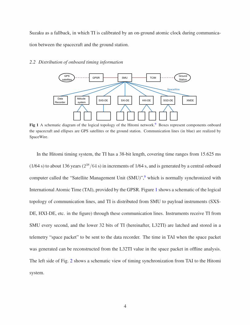
Fig 1 A schematic diagram of the logical topology of the Hitomi network.9 Boxes represent components onboard
the spacecraft and ellipses are GPS satellites or the ground station. Communication lines (in blue) are realized by
SpaceWire.
In the Hitomi timing system, the TI has a 38-bit length, covering time ranges from 15.625 ms
(1/64 s) to about 136 years (238/64 s) in increments of 1/64 s, and is generated by a central onboard
computer called the “Satellite Management Unit (SMU)”,9 which is normally synchronized with
International Atomic Time (TAI), provided by the GPSR. Figure 1 shows a schematic of the logical
topology of communication lines, and TI is distributed from SMU to payload instruments (SXS-
DE, HXI-DE, etc. in the figure) through these communication lines. Instruments receive TI from
SMU every second, and the lower 32 bits of TI (hereinafter, L32TI) are latched and stored in a
telemetry “space packet” to be sent to the data recorder. The time in TAI when the space packet
was generated can be reconstructed from the L32TI value in the space packet in offline analysis.
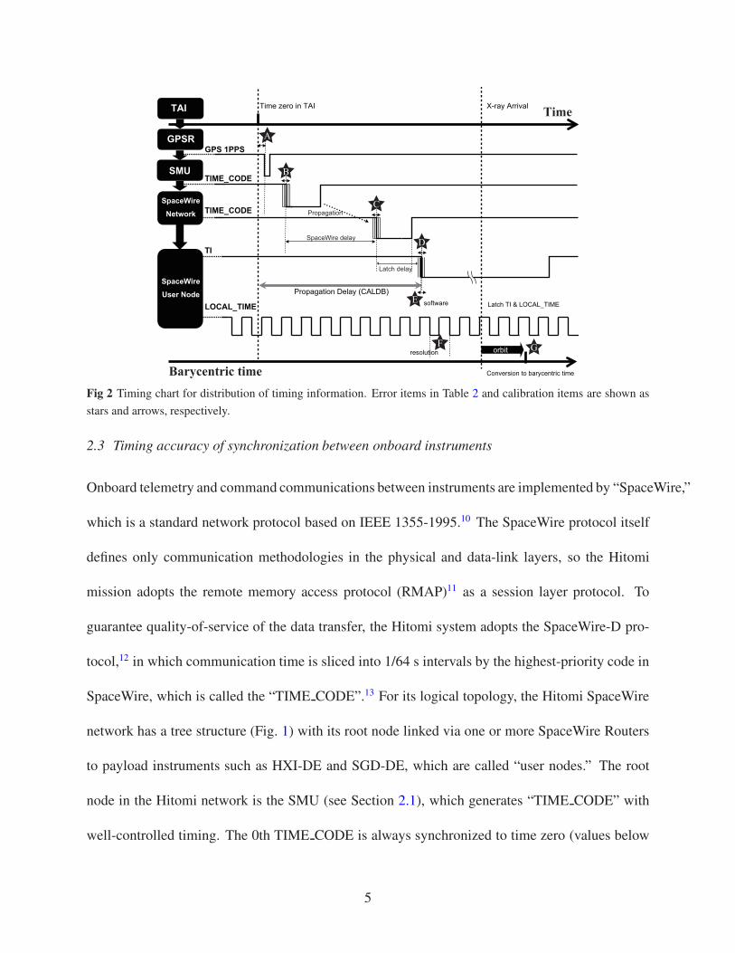
The left side of Fig. 2 shows a schematic view of timing synchronization from TAI to the Hitomi
system.
4
GPS 1PPS
TIME_CODE
TIME_CODE
TI
LOCAL_TIME
Propagation Delay (CALDB)
Time
Barycentric time
TAI
GPSR
SMU
SpaceWire
Network
SpaceWire
User Node
Propagation
SpaceWire delay
Time zero in TAI
Latch TI & LOCAL_TIME
Latch delay
software
resolution
X-ray Arrival
A
B
C
E
D
orbit
Conversion to barycentric time
GF
Fig 2 Timing chart for distribution of timing information. Error items in Table 2 and calibration items are shown as
stars and arrows, respectively.
2.3 Timing accuracy of synchronization between onboard instruments
Onboard telemetry and command communications between instruments are implemented by “SpaceWire,”
which is a standard network protocol based on IEEE 1355-1995.10 The SpaceWire protocol itself
defines only communication methodologies in the physical and data-link layers, so the Hitomi
mission adopts the remote memory access protocol (RMAP)11 as a session layer protocol. To
guarantee quality-of-service of the data transfer, the Hitomi system adopts the SpaceWire-D pro-
tocol,12 in which communication time is sliced into 1/64 s intervals by the highest-priority code in
SpaceWire, which is called the “TIME CODE”.13 For its logical topology, the Hitomi SpaceWire
network has a tree structure (Fig. 1) with its root node linked via one or more SpaceWire Routers
to payload instruments such as HXI-DE and SGD-DE, which are called “user nodes.” The root
node in the Hitomi network is the SMU (see Section 2.1), which generates “TIME CODE” with
well-controlled timing. The 0th TIME CODE is always synchronized to time zero (values below
5
the second are all zeros) of TAI. In other words, TIME CODE is used for synchronization of all
user nodes at an exact 64 Hz.
As described in Section 2.2, SMU distributes TI information to all user nodes. The upper 32 bits
of TI (covering above 1 s; hereinafter, U32TI) are distributed rather slowly (but within sub second)
from SMU to user nodes via the RMAP protocol, which is the same procedure as used in other
telemetry-and-command transmission. In contrast, the finer part of TI covering less than 1 s(6 bits)
is quickly broadcasted within the SpaceWire network using the same high-priority code as is used
for SpaceWire-D, that is, the TIME CODE, which carries 6-bit information. The Hitomi satellite
carries a large number of SpaceWire nodes (up to 120), and has main-and-redundant network paths,
making the SpaceWire system large and complex. Therefore, an understanding of the propagation
delay and jitter of the SpaceWire TIME CODE is key to estimating the timing accuracy. As an
example, the link rate of the Hitomi SpaceWire network at 50 or 20 MHz results in delay and jitter
on the order of about 1 µs (for details, see Sections 5.3), which are non-negligible for timing goals
of 35 µs (see Section 1).
2.4 Assignment of photons at fine timing resolutions
The arrival times of X-ray photons from astronomical objects are determined at user nodes con-
necting to X-ray sensors such as SXS, HXI, and SGD. The time resolution of TI (15.625 ms; see
Section 2.1) is insufficient for the timing goal of 35 µs (Section 1), although the timing accuracy
of TI distribution is sufficient on the order of about 1 µs (see Section 2.3). Therefore, clocks with
finer timing called “LOCAL TIME” are installed into each user node to refine resolutions to 5 µs,
61.0 µs, 25.6 µs, and 25.6 µs for SXS, SXI, HXI, and SGD, respectively, but with shorter time cov-
erage than TI, as summarized in Table 1. These time resolution values are within the requirement
6
for 350 µs accuracy for SXS, HXI, and SGD, and for a resolution of a few tens of milliseconds
for SGD-SHIELD (see Section 1). The time resolution for SXS is also sufficient for the best-
effort goal of 35 µs accuracy. The time resolutions of the HXI and the SGD (25.6 µs) may seem
to be a comparably larger fraction of the timing goal (35 µs). However, according to numerical
studies of realistic scientific cases for determining the coherent periods of periodic X-ray signals
from neutron-star pulsars, these instruments have sufficient performance to determine the period
of ∼ 100 ms at about less than 2 µs errors even from dimmer neutron stars below 1/1,000 of the
X-ray flux of the Crab pulsar.
Table 1 Summary of LOCAL TIME counters
Instrument Bit length Time resolution
SXS 28-bits 5 µs
SXI 32-bits 61.0 µs
HXI 32-bits 25.6 µs
SGD 32-bits 25.6 µs
SGD-SHIELD 32-bits 16 ms
Since a phase-locked loop to the TI counter requires the hardware resources at each user node,
the LOCAL TIME counters on Hitomi user node, except for the SXI, are implemented with free-
run clocks to reduce the hardware resources. In other words, LOCAL TIMEs are not synchronized
to TI and thus should be calibrated by TI with offline software (for details, see Section 3). Note
that the LOCAL TIME for the SXI is synchronized to L32TI on every arrival of a TIME CODE
at SXI-DE within 10 µs accuracy, so such offline calculations are not required for SXI. Therefore,
SXS, HXI, and SGD user nodes periodically (every 1 or 4 s) latch LOCAL TIME and U32TI
values simultaneously at TIME CODE = 0 (i.e., U32TI time zero) to generate a lookup table
between LOCAL TIME and TI. This lookup table for each user node is periodically stored in a
housekeeping space packet, with which the offline software recognizes the relation between user
7
node LOCAL TIMEs and TI.
When a user node acquires an X-ray event, the LOCAL TIME at detection is latched and
stored in an telemetry message. Such information is gathered for multiple events into a space
packet with a corresponding TI value. In summary, the time evolution of the relation between the
LOCAL TIME and the TI is stored in housekeeping telemetry, and the LOCAL TIME at X-ray
detection and the TI value when a space packet containing the detection is generated are stored in
the event telemetry. These three pieces of information in the telemetry are used in calculations of
the photon-arrival time by the offline software.
3 Software Design of Offline Time Assignment
3.1 Process flow
When all observation telemetry is ready on the ground, an automatic pipeline process starts con-
verting from raw telemetry data into the Flexible Image Transport System (FITS) format, a stan-
dard format for astrophysical use.14 The process then calculates calibrated physical values such as
time, pulse height invariant (photon energy), and coordinates from the raw telemetry values using
the calibration database, and writes them to FITS output files. Since Hitomi is a ”public observa-
tory,” the availability of such analysis software and calibration information for payload instruments
is very important. Thus, all Hitomi software and calibration databases are published in the “HEA-
soft” package and “CALDB” database, respectively, which are released to the public via NASA
GSFC.
Time assignment tasks are applied to raw telemetry in a pipeline process after conversion to
the FITS format. Time calculations are performed one-by-one for all FITS housekeeping and
science event files. The basic design concept for software time assignment tasks is common across
8
all instruments. Information from individual payload instruments is stored in the CALDB files.
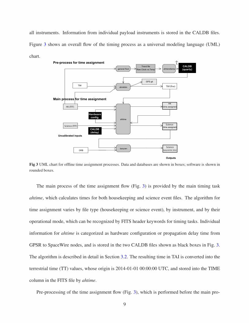
Figure 3 shows an overall flow of the timing process as a universal modeling language (UML)
chart.
Pre-process for time assignment
Main process for time assignment
Uncalibrated inputs
CALDB
(quartz)
Hardware
config.
CALDB
(delay)
Outputs
barycentric timebarycenORB
TIM
Science (FFF)
HK (FFF)
TIM (fine)
Science
Science
Fig 3 UML chart for offline time assignment processes. Data and databases are shown in boxes; software is shown in
rounded boxes.
The main process of the time assignment flow (Fig. 3) is provided by the main timing task
ahtime, which calculates times for both housekeeping and science event files. The algorithm for
time assignment varies by file type (housekeeping or science event), by instrument, and by their
operational mode, which can be recognized by FITS header keywords for timing tasks. Individual
information for ahtime is categorized as hardware configuration or propagation delay time from
GPSR to SpaceWire nodes, and is stored in the two CALDB files shown as black boxes in Fig. 3.
The algorithm is described in detail in Section 3.2. The resulting time in TAI is converted into the
terrestrial time (TT) values, whose origin is 2014-01-01 00:00:00 UTC, and stored into the TIME
column in the FITS file by ahtime.
Pre-processing of the time assignment flow (Fig. 3), which is performed before the main pro-
9
cess described above, is performed to handle the GPSR failure mode. GPS information can be
commonly treated among all telemetry and affects only the relation between Hitomi TI and the
corresponding TAI value. This relation is discontinuously measured during communications be-
tween the spacecraft and the ground station (as described in Section 2.1) and is stored in the TIM
FITS file shown in Fig. 3. Process by the ahmktim tool provides a continuous relation between the
TI and TAI regarding the GPS receiving status. A table refined by ahmktim is stored in the TIM-
fine file, which is used for individual time assignment by ahtime in the main process. The detailed
algorithm of ahmktim is described later in Section 3.3, and utilizes properties of the quartz clock
onboard SMU. A temperature dependence of a clock frequency of this quartz is stored in CALDB
(quartz), indicated by the black box in Fig. 3, and is scheduled for monthly onboard calibrations
by another pre-process (the ahtrendtemp tool).
The barycentric dynamical time (TDB; the photon arrival time converted from the celestial
sky position for light-travel times between the spacecraft and the center of the gravity of the solar
system) is required for further astrophysical uses, for example, when matching the arrival time of
photons in X-ray and radio observations.15 A barycentric correction tool (barycen) is provided as
an analysis tool, which is not applied in the pipeline process, because target positions for calcu-
lation must be set by users. The tool barycen is developed to be a mission-independent tool in
the HEAsoft package, which rely on the data formats containing specific information in a stan-
dard way, expecting that the time pre-computed is stored in the TIME column with standard FITS
keywords to identify the time system. Similarly it is expecting that the orbit is written in a file
with well-defined quantities (position and velocity) written in standard column names and units.
Historically, the barycentric correction tools were individually developed for previous missions in-
cluding ASCA and Suzaku,7 mainly because the orbital information required by the tool is stored
10
in a different format. The engine of the calculation of the barycentric correction in barycen is
a well trained algorithm derived as a standard routine for RXTE (Rossi X-ray Timing Explorer)
satellite and after used by Chandra, Swift, Suzaku, NuSTAR (Nuclear Spectroscopic Telescope
Array) and Fermi missions. The calculation is performed in the two steps, following the same
procedure used for the Suzaku satellite: 1) conversion from the TT value into the TDB value,
considering the movement of the Earth under the gravitational potential of the Sun, 2) correction
of the time delay of the light travel time between the spacecraft and the solar system barycenter,
where the geometrical position of the spacecraft is identified by the orbital elements in the orbit
file, considering the general relativity effects by the Sun and planets. The tool supports the solar
system ephemerides of JPL-DE200. After the conversion, the FITS header keyword TIMEREF
is changed from ’LOCAL’ to ’SOLARSYSTEM.’ The largest shifts (about 8 minutes maximum)
occur in step 2, but this calculation is well established. The largest systematic error arises in step
1, from positional accuracy for the orbital element of the spacecraft. Such systematic errors are
discussed in Section 4.
3.2 Algorithm for the time assignment process ahtime
Calculations at the main processing stage using ahtime are simple. In calculating times for the
housekeeping FITS files, the TAI system time is calculated from the input of L32TI, which is one
value per one row in the FITS file using the TIM file (i.e., the relation between L32TI and TAI,
as defined in Section 3.1). The ahtime process takes from the TIM file two points before and
two after the input L32TI and linearly interpolates them to calculate the corresponding TAI value.
Since the TIME column in the Hitomi FITS file is defined as the number of seconds from 2014-
01-01 00:00:00 UTC, whereas the origin for TAI is 1980-01-06 00:00:19 UTC, the calculated TAI
11
is converted to the ASTRO-H time system by subtracting the offset of the two origins; i.e., the
ASTRO-H time in TT is TI− 1, 072, 569, 616 sec, where the origin of TI is TAI− 19 sec.
When calculating the TIME of science event FITS files from payload instruments using ahtime,
LOCAL TIME counters, described in Section 2.4, are also considered. Since LOCAL TIME rep-
resents a finer timing when a photon is detected by the instrument, the TIME in the science event
FITS file is defined at the event detection timing at finer time resolutions. The calculation contains
the two lookup processes described above. The first lookup process uses the relation between LO-
CAL TIME and U32TI monitored in the housekeeping file of the instrument to calculate the L32TI
corresponding to the input LOCAL TIME. The second lookup process is the same procedure as
that in the housekeeping data, from L32TI to TAI using the TIM file. Since the propagation delay
of TAI information from GPSR to the instrument’s SpaceWire node is not negligible as compared
with the time resolution (see Section 2.3), the final step in time assignment for science event files
by ahtime is to add the propagation delay to the TAI value obtained above. As a result, the ahtime
calculation retrieves the time in TAI with finer resolution than TI at the X-ray detection timing by
each event, which can be converted to the ASTRO-H time system as was done for the housekeeping
data.
To perform the above process, individual instrument information is stored in the CALDB files
(black boxes in Fig. 3) and is used by ahtime. The stored information is 1) the CALDB hardware
configuration, which describes hardware configuration parameters for LOCAL TIME as summa-
rized in Table 1 and the attribute names in the telemetries of instrument timing counters, and 2) the
CALDB propagation delay, which describes the propagation delay time of TAI information from
GPSR to the SpaceWire user node via SMU and the SpaceWire network (Section 2.3).
12
3.3 Treatment of GPS lock-off data, ahmktim and ahtrendtemp
As described in Section 3.1, pre-processing of the time assignment flow in Fig. 3 checks the GPSR
status to calculate the relation between TI and TAI, to support the fallback case in the event of
GPSR failure as required in Section 1.
The GPSR onboard Hitomi is designed to always capture several GPS satellites on orbit (here-
inafter, we call this GPS-ON mode), so cases where GPSR detects no GPS carry signal (hereinafter,
GPS-OFF mode) should be rare. In the design policy for the Hitomi spacecraft, the data acquisition
system should be robust for any single-point failure, such as a completely GPS-OFF mode. At the
same time, the SpaceWire-D protocol used in the Hitomi data acquisition system (see Section 2.3)
requires that the TIME CODE should not jump and that the time interval between TIME CODEs
(time slot in SpaceWire-D; 16 ms) should be stable to within a few hundred microseconds. The
SMU is thus designed to follow the above requirements. The TI is always synchronized to the TAI
provided by the GPSR in GPS-ON mode and, even in GPS-OFF mode, the SMU keeps generating
the TI using the free-run clock onboard SMU and keeps distributing TIME CODEs. When the
GPS-OFF mode switches to GPS-ON mode, the SMU starts synchronization of TI to TAI, which
takes a few to few tens of seconds as a transition mode, and then the TI is synchronized to TAI
again in GPS-ON mode. The transition mode normally happens at the beginning of operations
(such as initial on-orbit operations), but it never happens when GPS-OFF mode continues forever.
As briefly described in Section 3.1, the ahmktim process refines the TIM file, which describes
the continuous relation between the TI and TAI, considering the GPSR status. This relation is
simple in normal GPS-ON mode, because the TI is synchronized to TAI. On the other hand, the
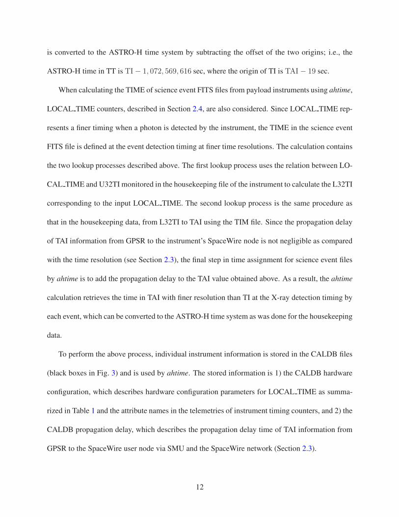
calculation during GPS-OFF mode has two-step corrections of GPS-OFF data as schematically
13
shown in Fig. 4 when the GPSR status changes from GPS-ON to GPS-OFF, and then back to
GPS-ON mode. The raw data obtained during GPS-ON and GPS-OFF modes are shown in red
and magenta, respectively, and a wavy trend can be seen during the GPS-OFF mode from TAI =
(x) to (y). Such fluctuations in TI are generated by a free-run clock on the SMU whose frequency
shifts with temperature drift. As the first step of GPS-OFF data correction, such short-term trends
are corrected by the temperature of the SMU quartz, as monitored in the housekeeping data using
the CALDB (quartz) file defined in Section 3.1, shown as black points in Fig. 4. In the second
correction step for GPS-OFF data, the red points during GPS-ON mode are used as anchor points
where the TI is synchronized to TAI, and to adjust the beginning point (x) and the end point (y) of
the GPS-OFF data to the two anchor points. In the case of Fig. 4, the beginning point (x) is already
connected to the last point of the former GPS-ON data, but a tentative jump between black and
red points can be seen at (y), which is then corrected as a long-term correction. Finally, a more
stable trend than the original data (magenta) is obtained as the blue points in Fig. 4. The red and
blue points are output from ahmktim. Note that if no anchor points exist during the observation
like in the case of complete GPS-OFF mode under permanent GPSR failure, ahmktim searches for
other anchor points from the original TIM file, which describes the relation between TI and TAI
as discontinuously measured during ground contacts. This function provides a fallback plan that
successfully worked for Suzaku.
Another pre-processing of time assignments in Fig. 3 records the temperature dependence of
the SMU quartz clock in the CALDB (quartz) file as measured on orbit. Information obtained on
orbit is limited, so detailed measurements of the temperature dependence of the SMU quartz are
performed on the ground, the results of which are described in Section 5.1. The SMU measures
the frequency of the onboard quartz clock, referring to the GPS signals from GPSR. This function
14
104000
106000
108000
110000
112000
114000
116000
TAI
L3
2T
I
raw data
short-term corrected
short-/long-term corrected
GPS ON GPS ONGPS OFF
(x)
(y)
Fig 4 Schematic view of calculating the relation between TAI and L32TI during GPS-OFF mode by ahmktim. Raw
data obtained during GPS-ON and GPS-OFF modes are shown in red and magenta, respectively. Black points are
intermediate data in the ahmktim calculations, where short-term temperature drifts were corrected. Blue data points
are final task outputs, whose long-term shifts are corrected to match the final point (y).
can be activated by an operation command during GPS-ON mode, but note that the measurement
does not work during GPS-OFF mode. Such operations are scheduled once per month on orbit.
Therefore, pre-processing by ahtrendtemp is scheduled to be triggered monthly. The ahtrendtemp
process picks up temperature and self-measured frequency information of the SMU quartz from
housekeeping telemetry, and generates the relation between temperature and frequency. In this
process, same temperature may appear many times, and thus the ahtrendtemp process calculates the
average of the frequency values within the defined temperature bins. After the averaging operation,
the results are stored in an extension of the CALDB file for the quartz frequency.
15
4 Management of the Timing Uncertainties
4.1 Items on timing uncertainties
Under the hardware and software designs for the timing system (see Sections 2 and 3), timing
performance should meet the requirements for the timing system, namely, 350 or 35 µs in absolute
time as a basic requirement or a mission goal, respectively (see Section 1). To more precisely
control overall uncertainty in the timing system, seven items are identified as those which may
reduce timing accuracy. These items are indicated by stars in the timing chart of the Hitomi timing
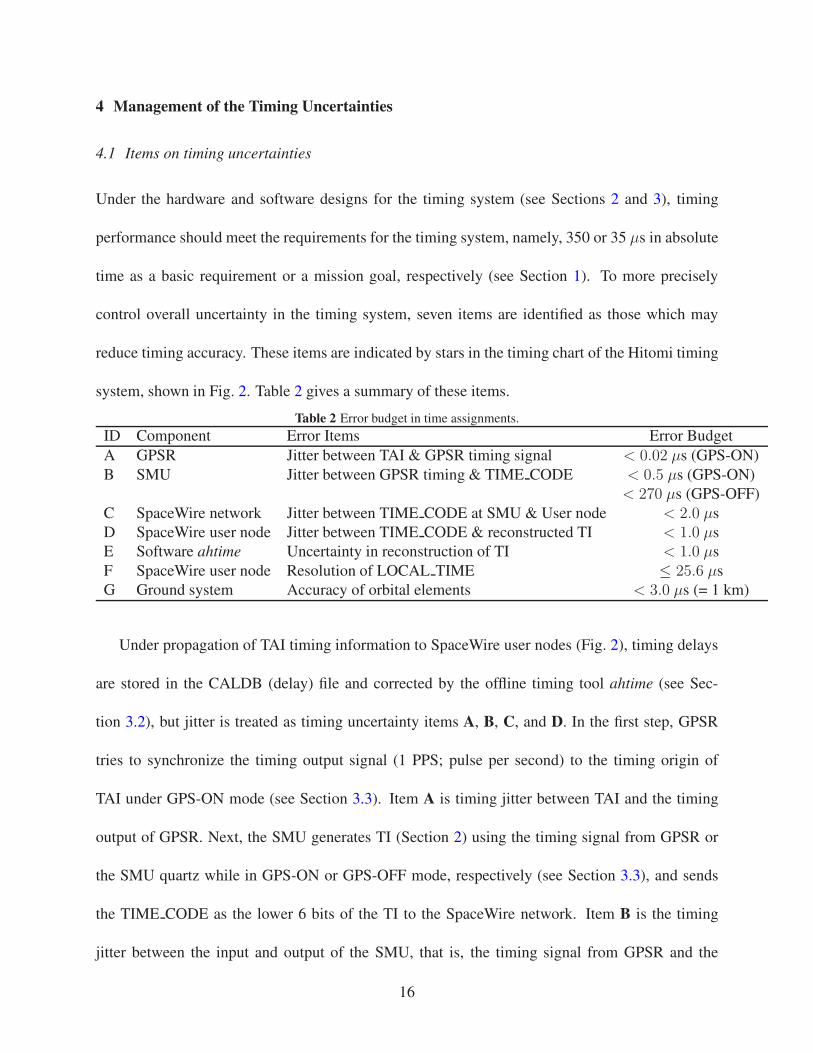
system, shown in Fig. 2. Table 2 gives a summary of these items.
Table 2 Error budget in time assignments.
ID Component Error Items Error Budget
A GPSR Jitter between TAI & GPSR timing signal < 0.02 µs (GPS-ON)
B SMU Jitter between GPSR timing & TIME CODE < 0.5 µs (GPS-ON)
< 270 µs (GPS-OFF)
C SpaceWire network Jitter between TIME CODE at SMU & User node < 2.0 µs
D SpaceWire user node Jitter between TIME CODE & reconstructed TI < 1.0 µs
E Software ahtime Uncertainty in reconstruction of TI < 1.0 µs
F SpaceWire user node Resolution of LOCAL TIME ≤ 25.6 µs
G Ground system Accuracy of orbital elements < 3.0 µs (= 1 km)
Under propagation of TAI timing information to SpaceWire user nodes (Fig. 2), timing delays
are stored in the CALDB (delay) file and corrected by the offline timing tool ahtime (see Sec-
tion 3.2), but jitter is treated as timing uncertainty items A, B, C, and D. In the first step, GPSR
tries to synchronize the timing output signal (1 PPS; pulse per second) to the timing origin of
TAI under GPS-ON mode (see Section 3.3). Item A is timing jitter between TAI and the timing
output of GPSR. Next, the SMU generates TI (Section 2) using the timing signal from GPSR or
the SMU quartz while in GPS-ON or GPS-OFF mode, respectively (see Section 3.3), and sends
the TIME CODE as the lower 6 bits of the TI to the SpaceWire network. Item B is the timing
jitter between the input and output of the SMU, that is, the timing signal from GPSR and the
16
TIME CODE, respectively. Third, the TIME CODE is distributed via the SpaceWire network,
and user nodes reconstruct the TI from TIME CODE and the upper 32 bits of the TI obtained via
RMAP (see Section 2). Item C is the jitter of the timing of TIME CODE between, before, and after
propagation via the SpaceWire network, and item D is jitter in synchronization of TIME CODE to
the TI reconstructed on the user node.
Item E is systematic error in the interpolation of TIs by the timing task ahtime (see Section 3.2),
and item F is the time resolution of instruments as summarized in Table 1. Item G, which is ac-
curacy of the orbital determination of the spacecraft, is provided for users who require barycentric
time in their analyses. The barycentric time is calculated by the tool barycen (see Section 3.1),
which requires the target position and the orbital elements of the spacecraft.
4.2 Error budget for timing uncertainties
To control and maintain overall timing uncertainties, the error budgets for all items identified in
Section 4.1 are defined as in Table 2. As defined in Section 1, the requirements and goals for SXS,
HXI, and SGD are 350 µs and 35 µs, and item F is defined in Table 1 (5 µs for SXS and 25.6 µs for
HXI and SGD). Therefore, the remaining 324 and 9 µs are distributed to other items in GPS-OFF
and GPS-ON modes, respectively. Such GPS modes only affect items A and B; the error budget of
item A is valid only in GPS-ON mode, and that of item B is defined by the GPS mode. Item G (the
orbital determination accuracy) becomes worse in GPS-OFF mode than that in GPS-ON mode, but
the budget include both modes.
The error budgets for items A and D come from hardware design specification sheets of the
GPSR and the SpaceWire user node (digital electronics; DE), respectively. The budget for item B
in GPS-ON mode also comes from the hardware design, and that for GPS-OFF mode is defined
17
as 270 µs from the actual best-case performance of the Suzaku satellite.7 The budget for item G
is the minimum requirement for the orbital determination group of the spacecraft operation. The
remaining items C and E are defined as 2.0 and 1.0 µs at maximum from a rough estimations from
the system design and the software algorithm, respectively.
5 Verification of Timing Performance
5.1 Ground measurement of temperature dependence on quartz frequency
As described in Section 3.3, temperature dependence of the quartz clock onboard SMU is described
in the CALDB (quartz) and is used by ahmktim for time calculations in GPS-OFF mode. The SMU
has a function for self-measurement of this calibration item, but the operations are limited on orbit.
Therefore, a) detailed measurements of temperature dependence of the clock frequency and b)
functional tests of self-measurement in the flight configuration are performed on the ground before
launch.
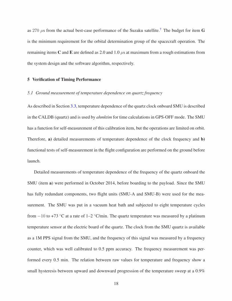
Detailed measurements of temperature dependence of the frequency of the quartz onboard the
SMU (item a) were performed in October 2014, before boarding to the payload. Since the SMU
has fully redundant components, two flight units (SMU-A and SMU-B) were used for the mea-
surement. The SMU was put in a vacuum heat bath and subjected to eight temperature cycles
from −10 to +73 ◦C at a rate of 1–2 ◦C/min. The quartz temperature was measured by a platinum
temperature sensor at the electric board of the quartz. The clock from the SMU quartz is available
as a 1M PPS signal from the SMU, and the frequency of this signal was measured by a frequency
counter, which was well calibrated to 0.5 ppm accuracy. The frequency measurement was per-
formed every 0.5 min. The relation between raw values for temperature and frequency show a
small hysteresis between upward and downward progression of the temperature sweep at a 0.9%
18
0.999960
0.999965
0.999970
0.999975
0.999980
0.999985
0.999990
0.999995
1.000000
-10 0 10 20 30 40 50 60 70
Temperature
Fre
qu
ency
(M
Hz)
SMU-A (before boarding)
SMU-B (before boarding)
SMU-A (onboard)
SMU-B (onboard)
Fig 5 Temperature dependence of the 1-MHz quartz-frequency in SMU-A and SMU-B onboard the Hitomi satellite.
Detailed measurements from before mounting on the spacecraft are shown in green and magenta for SMU-A and
SMU-B, respectively. Confirmation measurements during the thermal vacuum test on ground are shown in blue and
red for SMU-A and SMU-B, respectively.
level, so the measured points are averaged within a 1.0 Hz range when more than three points
exist in that range. Figure 5 shows the results for SMU-A and SMU-B in green and magenta,
respectively. This tables are recorded in the CALDB (quartz) file for use by ahmktim (Fig. 3).
Functional test of self-measurement of the temperature dependence of the SMU quartz (item b)
was performed in spacecraft thermal vacuum test from June to July 2015, when the spacecraft was
in its flight configuration. During spacecraft thermal vacuum testing, hot and cold temperature
environments were prepared for functional testing of onboard instruments. The self-measurement
function of the temperature dependence of the SMU-A quartz was activated 30 times (for 16 s
each) in GPS-ON mode during transition from hot to cold mode. The same function for SMU-B
was also checked 9 times during cold mode. Figure 5 shows the results for SMU-A and SMU-B
in blue and red, respectively. These results are consistent with the detailed measurement described
19
above to within a 0.5 ppm level, which is sufficient for correction by ahmktim.
In addition to items a and b above, the temperature dependence can be roughly verified in
the transition mode between the GPS-OFF to GPS-ON modes (see Section 3.3). This transition
happened once on the ground during spacecraft thermal vacuum testing in July 2015 and once on
orbit in February 2016. On the ground, the GPSR mode changed from GPS-ON to GPS-OFF,
then to GPS-ON again. The duration of GPS-OFF mode was 14,912 s and the temperature of the
SMU-A was about 32.8 ◦C, which corresponds to a 1PPS quartz frequency of about 0.9999797 Hz.
Therefore, the free-run TI is expected to shift about 0.3034 s (19.4 ticks of L32TI) from TAI at
the end of GPS-OFF mode, and 20.1 ticks of L32TI were actually observed, for consistency at
a 4% level. On orbit, the spacecraft operated in GPS-OFF mode from just after launch (17 Feb
2016) until when the GPS synchronization function was turned on (00:35 29 Feb 2016 UTC).
From 03:52:32 18 Feb 2016 UTC to 00:35:18 29 Feb 2016, L32TI shifted about 986.651 ticks,
corresponding to 15.42 s. During this period, which lasted about 938 ks, the SMU temperature
was almost always about 26.3 ◦C, at which the quartz frequency should be 0.9999839 Hz from
Fig. 5, and thus about a 15.11 s shift is expected at this frequency over about 938 ks. Therefore,
the temperature dependence of the frequency of SMU-A quartz was also verified at about a 2%
level here.
5.2 Ground measurement of Item B: Delay from GPSR to SMU
The measurement of item B in the error budget (Table 2) was performed during the first integration
test in October 2013 when the GPSR, SMU, SpaceWire network, and SpaceWire user nodes were
in their flight configuration. The goal was to measure the timing delay and jitter between the input
and output of SMU, which are the GPSR 1PPS signal and the TIME CODE. The former signal can
20
be easily seen with an oscilloscope, but the latter is difficult to handle because the SpaceWire line
is also used for communication of many commands and telemetries. Therefore, a simple converter
from the SpaceWire TIME CODE to a single digital pulse that is detectable by an oscilloscope
was prepared for this measurement. Here, we call this converter the “TIME CODE handler.”
Before main measurements in the flight configuration, the timing delay and jitter of the TIME CODE
handler were measured using a commercial GPSR. Measurements were performed over 25,169 tri-
als under a SpaceWire link rate of 48 MHz at the same rate as the actual SMU SpaceWire port. The
results showed that the time delay becomes 387± 6.4 ns with 1-sigma error. Note that, among this
value, 219 ns were spent in recognizing the full signal length of TIME CODE by the TIME CODE
handler, there was about a 2-ns delay due to SpaceWire cables, and that jitter by this GPSR is neg-
ligible (within 1 ns).
network idle
network busy
Delay time [ns]600 700 800 900 1000 1100 1200
Nu
mb
er
of m
ea
su
rem
en
ts
10
20
30
40
60
70
80
50
Fig 6 Time delay within SMU from GPSR 1PPS signal to TIME CODE emitted from SMU. Intrinsic delay of the
measurement system (387 ns) is included in the horizontal axis.
In main measurements of item B, the 1PPS signal from the GPSR was picked up from the
communication line between SMU and GPSR, and the TIME CODE from the SMU was captured
21
by the TIME CODE handler, pre-measured above, from the communication line between the SMU
and the SpaceWire router in the network. These two signals were detected by an oscilloscope,
and the time delay and jitter between the two were measured. The measurement is performed in
two modes, when the SpaceWire network is unoccupied and when it is nearly fully occupied by
communications between the components (hereinafter, these states are called “idle” and “busy,”
respectively). In total, 1,910 and 1,619 measurements were performed in the idle and busy states,
respectively. Figure 6 shows the results. In that figure, the horizontal axis includes the delay of the
TIME CODE handler, 387 ns. Numerically, the results were 914 ± 46 ns and 920 ± 47 ns in the
idle and busy states, respectively, with 1-sigma errors. In summary, after subtracting the timing
properties of the TIME CODE handler, the timing delay at SMU becomes 530± 46 ns. The delay
value of 530 ns is included in the CALDB (delay) file (see Fig. 3), which is used by the offline
process with ahtime. Since the jitter value for the error budget is defined as the 3-sigma, item B
becomes about 137 ns, which satisfies the error budget (0.5 µs) in Table 2.
5.3 Ground measurement of items C and D: Propagation time of TIME CODE
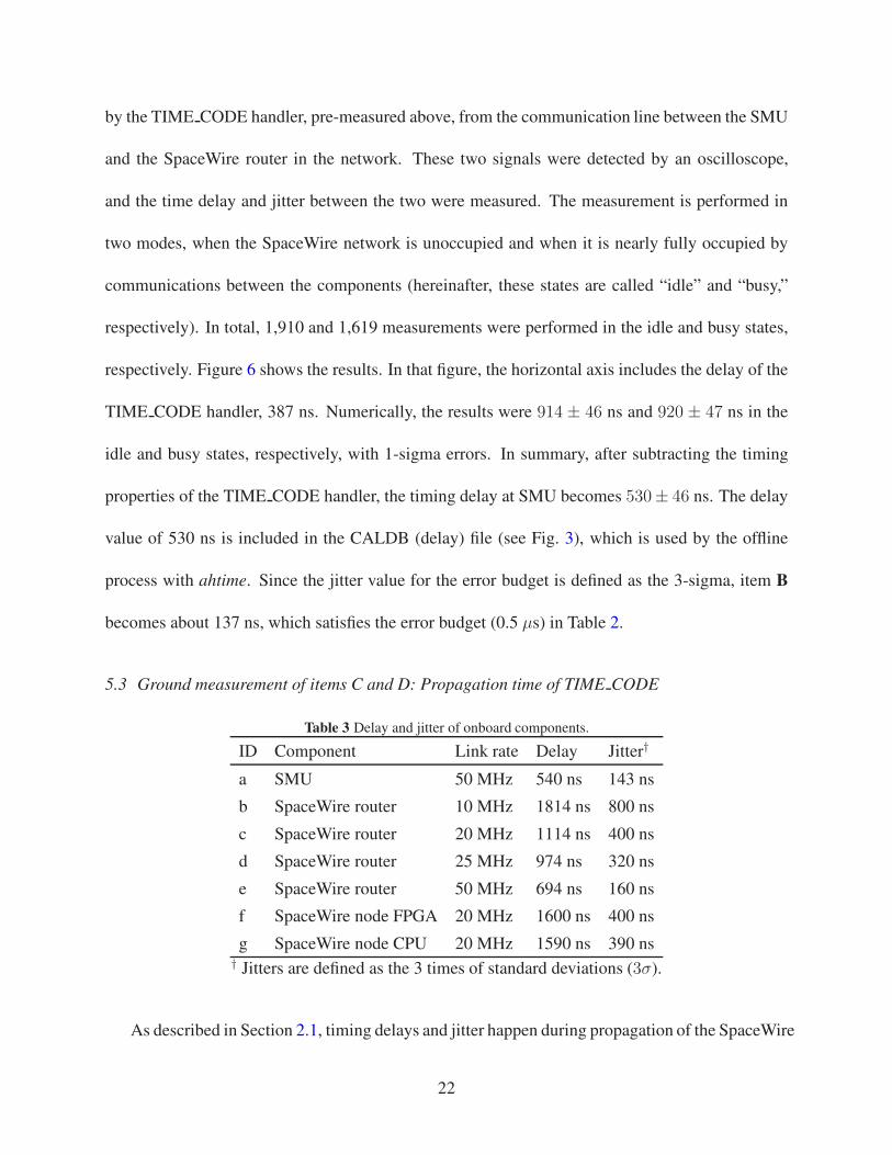
Table 3 Delay and jitter of onboard components.
ID Component Link rate Delay Jitter†
a SMU 50 MHz 540 ns 143 ns
b SpaceWire router 10 MHz 1814 ns 800 ns
c SpaceWire router 20 MHz 1114 ns 400 ns
d SpaceWire router 25 MHz 974 ns 320 ns
e SpaceWire router 50 MHz 694 ns 160 ns
f SpaceWire node FPGA 20 MHz 1600 ns 400 ns
g SpaceWire node CPU 20 MHz 1590 ns 390 ns† Jitters are defined as the 3 times of standard deviations (3σ).
As described in Section 2.1, timing delays and jitter happen during propagation of the SpaceWire
22
TIME CODE through the SpaceWire network tree from the SMU to user nodes. The jitter values
correspond to item C in Table 2 (see Section 4.1), and all the delay values are listed in the CALDB
(delay) file, which is used by the offline software ahtime (see Section 3.2). Such delay and jitter
values can be measured by probing many points in the SpaceWire network tree, but the number of
points is limited in on-ground tests in the full satellite flight configuration due to the tight sched-
ule before launch. Therefore, delay and jitter values of each element in the SpaceWire network
were first measured as summarized in Table 3, and the overall delay and jitter were estimated by
a simple propagation simulator of TIME CODE under the SpaceWire network configuration (i.e.,
routing and the link rate) using pre-measured values of elements. The overall delay time is just a
linear sum of each delay (Table 3) in the routing path of the instruments listed in Table 4, but jitter
is estimated by Monte Carlo simulation of the propagation of TIME CODE hops at each node.
Table 4 shows the results of estimations of delay and jitter values.
Table 4 Delay and jitter estimated for instruments.
Instrument Delay Jitter Source Routing† Destination
SXS 6092 ns 767 ns GPSR -a-e-e-d-f-g- f
SXS-FW 3742 ns 270 ns GPSR -a-e-e-b- SXS-FW
SXI 4502 ns 1041 ns GPSR -a-e-e-d-f- f
HXI-1 3838 ns 755 ns GPSR -a-e-d-(cable)-f- f
HXI-2 4505 ns 766 ns GPSR -a-e-e-d-(cable)-f- f
CAMS 3048 ns 717 ns GPSR -a-e-b- f
SGD-1 3835 ns 476 ns GPSR -a-e-d-f- f
SGD-2 4500 ns 493 ns GPSR -a-e-e-d-f- f† IDs (a,b,c,d,e,f,g) are defined in Table 3.
To verify the delay and jitter values estimated in Table 4, two paths from SMU to SGD-1 DE
were selected and measured during the first integration test in October 2013. Table 5 lists the
probe points, which are located at the point just after the SMU and before the CPU node or FPGA
23
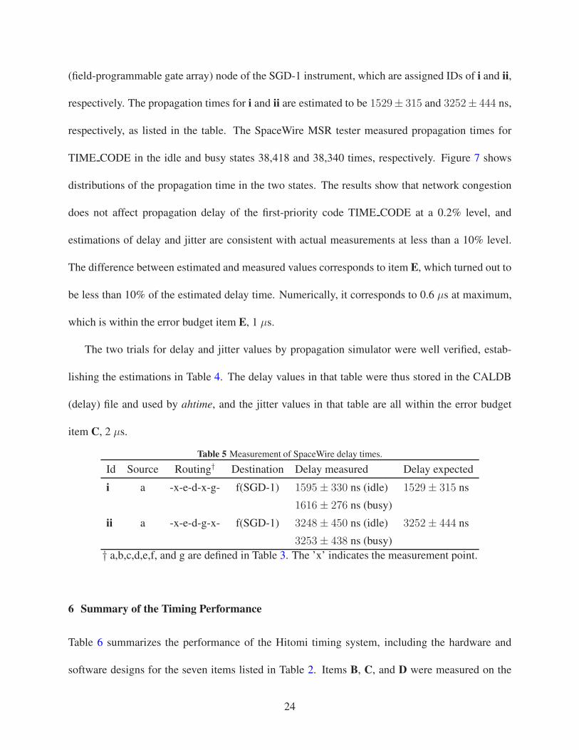
(field-programmable gate array) node of the SGD-1 instrument, which are assigned IDs of i and ii,
respectively. The propagation times for i and ii are estimated to be 1529± 315 and 3252± 444 ns,
respectively, as listed in the table. The SpaceWire MSR tester measured propagation times for
TIME CODE in the idle and busy states 38,418 and 38,340 times, respectively. Figure 7 shows
distributions of the propagation time in the two states. The results show that network congestion
does not affect propagation delay of the first-priority code TIME CODE at a 0.2% level, and
estimations of delay and jitter are consistent with actual measurements at less than a 10% level.
The difference between estimated and measured values corresponds to item E, which turned out to
be less than 10% of the estimated delay time. Numerically, it corresponds to 0.6 µs at maximum,
which is within the error budget item E, 1 µs.
The two trials for delay and jitter values by propagation simulator were well verified, estab-
lishing the estimations in Table 4. The delay values in that table were thus stored in the CALDB
(delay) file and used by ahtime, and the jitter values in that table are all within the error budget
item C, 2 µs.
Table 5 Measurement of SpaceWire delay times.
Id Source Routing† Destination Delay measured Delay expected
i a -x-e-d-x-g- f(SGD-1) 1595± 330 ns (idle) 1529± 315 ns
1616± 276 ns (busy)
ii a -x-e-d-g-x- f(SGD-1) 3248± 450 ns (idle) 3252± 444 ns
3253± 438 ns (busy)
† a,b,c,d,e,f, and g are defined in Table 3. The ’x’ indicates the measurement point.
6 Summary of the Timing Performance
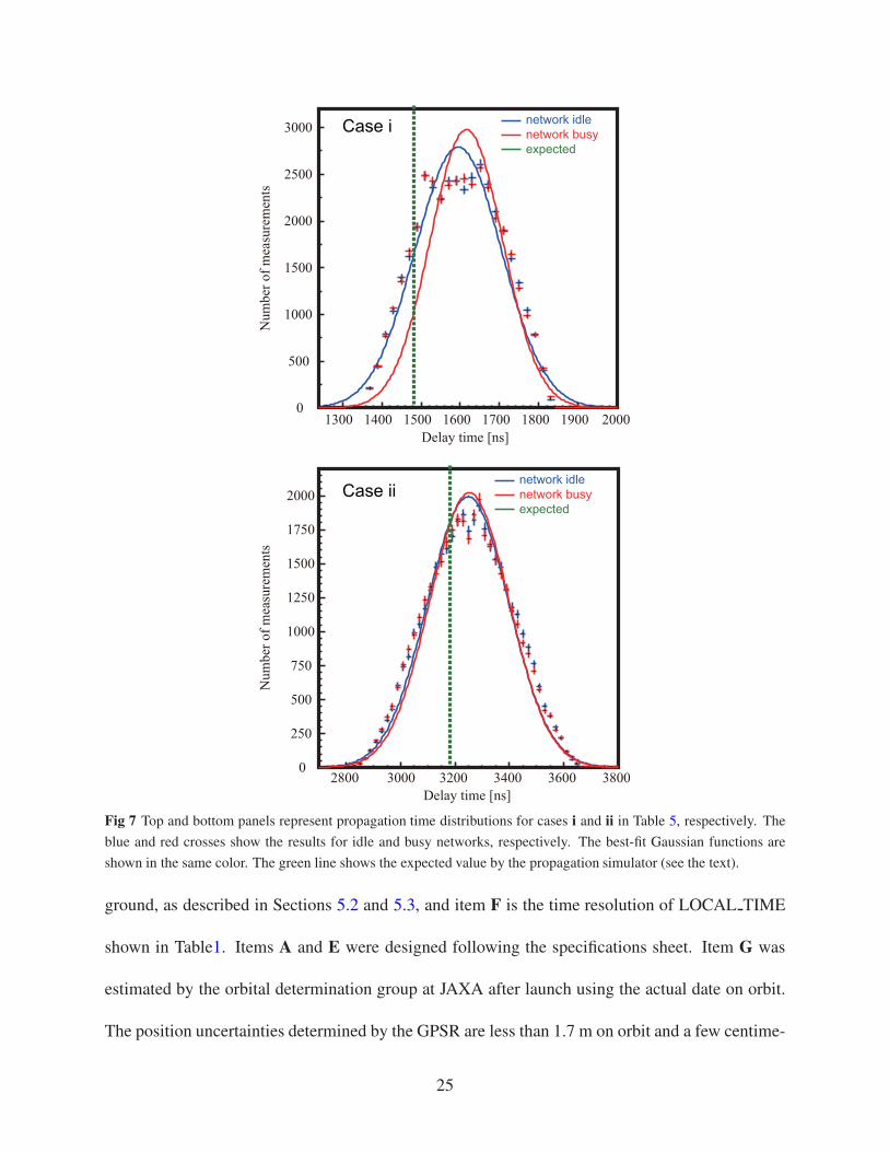
Table 6 summarizes the performance of the Hitomi timing system, including the hardware and
software designs for the seven items listed in Table 2. Items B, C, and D were measured on the
24
0
500
1000
1500
2000
2500
3000
1300 1400 1500 1600 1700 1800 1900 2000
network idle
network busy
expected
Delay time [ns]
Num
ber
of
mea
sure
men
ts
0
250
500
750
1000
1250
1500
1750
2000
2800 3000 3200 3400 3600 3800
Delay time [ns]
Num
ber
of
mea
sure
men
ts
network idle
network busy
expected
Case i
Case ii
Fig 7 Top and bottom panels represent propagation time distributions for cases i and ii in Table 5, respectively. The
blue and red crosses show the results for idle and busy networks, respectively. The best-fit Gaussian functions are
shown in the same color. The green line shows the expected value by the propagation simulator (see the text).
ground, as described in Sections 5.2 and 5.3, and item F is the time resolution of LOCAL TIME
shown in Table1. Items A and E were designed following the specifications sheet. Item G was
estimated by the orbital determination group at JAXA after launch using the actual date on orbit.
The position uncertainties determined by the GPSR are less than 1.7 m on orbit and a few centime-
25
Table 6 Summary of performance by the timing error budgets.
ID† Component Performance
A GPSR 0.01 µs
B SMU 0.14 µs (GPS-ON)
C SpaceWire network 0.3 – 1.0 µs (Table 4)
D SpaceWire user node < 1.0 µs
E Delay correction < 0.6 µs
F Time resolution 5 or 25.6 µs (Table 1)
G Orbit 0.3 ns (GPS-ON), 0.5 µs (GPS-OFF)† IDs (A, B, C, D, E, F, G) are defined in Table 2.
ters by the offline determination process on the ground under the GPS-ON mode. The accuracy
becomes worse in the GPS-OFF mode when the orbital elements are determined by measurements
of the position and velocity of the spacecraft from the ground station via ranging operations, but it
is about 150 m. Therefore, item G is negligible for the timing system both in GPS-ON and -OFF
modes. In summary, all seven items satisfy the error budget in Table 2.
Acknowledgments
The authors would like to thank all the science and engineering members of the Hitomi team for
their continuous contributions toward the development of instruments, software, and spacecraft
operations. This work was supported in part by Grants-in-Aid for Scientific Research (B) from
the Ministry of Education, Culture, Sports, Science and Technology (MEXT) (No. 23340055 and
No. 15H00773, Y. T).
References
1 T. Takahashi, M. Kokubun, K. Mitsuda, et al., “The ASTRO-H (Hitomi) x-ray astronomy
satellite,” in Space Telescopes and Instrumentation 2016: Ultraviolet to Gamma Ray, Pro-
ceedings of the SPIE 9905, 99050U (2016).
26
2 K. Mitsuda, R. L. Kelley, K. R. Boyce, et al., “The high-resolution x-ray microcalorimeter
spectrometer system for the SXS on ASTRO-H,” in Space Telescopes and Instrumentation
2010: Ultraviolet to Gamma Ray, Proceedings of the SPIE 7732, 773211 (2010).
3 H. Tsunemi, K. Hayashida, T. G. Tsuru, et al., “Soft x-ray imager (SXI) onboard ASTRO-H,”
in Space Telescopes and Instrumentation 2010: Ultraviolet to Gamma Ray, Proceedings of
the SPIE 7732, 773210 (2010).
4 G. Sato, M. Kokubun, K. Nakazawa, et al., “The Hard X-ray Imager (HXI) for the ASTRO-
H Mission,” in Space Telescopes and Instrumentation 2014: Ultraviolet to Gamma Ray,
Proceedings of the SPIE 9144, 914427 (2014).
5 Y. Fukazawa, H. Tajima, S. Watanabe, et al., “Soft gamma-ray detector (SGD) onboard the
ASTRO-H mission,” in Space Telescopes and Instrumentation 2014: Ultraviolet to Gamma
Ray, Proceedings of the SPIE 9144, 91442C (2014).
6 T. Kouzu, K. Iwase, Y. Mishima, et al., “The time assignment system of astro-h,” in 2011
IEEE Nuclear Science Symposium Conference Record, 163–166 (2011).
7 Y. Terada, T. Enoto, R. Miyawaki, et al., “In-Orbit Timing Calibration of the Hard X-Ray
Detector on Board Suzaku,” Publications of the Astronomical Society of Japan 60, S25–S34
(2008).
8 Y. Tanaka, H. Inoue, and S. S. Holt, “The X-ray Astronomy Satellite ASCA”, in Publ. Astron.
Soc. Japan, 46, L37 (1994)
9 M. Ozaki, T. Takahashi, M. Kokubun, et al., “SpaceWire Driven Achitecture for the ASTRO-
H Satellite,” in SpaceWire-2010, Proceedings of the 3rd International SpaceWire Conference,
1, 445 (2010).
27
10 IEEE Computer Society, “IEEE Standard for Heterogeneous Interconnect (HIC) (Low-Cost,
Low-Latency Scalable Serial Interconnect for Parallel System Construction),” IEEE Std
1355-1995 5449182, – (1996).
11 S. Parkes and C. McClements, “Space Wire Remote Memory Access Protocol,” in DASIA
2005 - Data Systems in Aerospace, ESA Special Publication 602, 18.1 (2005).
12 S. Parkes, D. Gibson, and A. Ferrer, “SpaceWire-D: Deterministic Data Delivery Over
SpaceWire,” in DASIA 2014 - DAta Systems In Aerospace, ESA Special Publication 725,
30 (2014).
13 S. Parkes, “The Operation and Uses of the SpaceWire TimeCode,” in Proceedings of the
International SpaceWire Seminar, 1, 1 (2003).
14 R. J. Hanisch, A. Farris, E. W. Greisen, et al., “Definition of the Flexible Image Transport
System (FITS),” Astronomy and Astrophysics 376, 359–380 (2001).
15 Hitomi collaboration (corresponding authors; Y. Terada, T. Enoto, S. Koyama, et al.), “X-ray
studies of Giant Radio Pulses from Crab pulsar with Hitomi,” Publications of the Astronomi-
cal Society of Japan 70, in press (arXiv:1707.08801) (2018).
Yukikatsu Terada is an associated professor at Saitama University. He received his BS and MS
degrees in physics, and PhD degree in science from the University of Tokyo in 1997, 1999, and
2002, respectively.
Biographies and photographs of the other authors are not available.
28
List of Figures
1 A schematic diagram of the logical topology of the Hitomi network.9 Boxes rep-
resent components onboard the spacecraft and ellipses are GPS satellites or the
ground station. Communication lines (in blue) are realized by SpaceWire.
2 Timing chart for distribution of timing information. Error items in Table 2 and
calibration items are shown as stars and arrows, respectively.
3 UML chart for offline time assignment processes. Data and databases are shown in
boxes; software is shown in rounded boxes.
4 Schematic view of calculating the relation between TAI and L32TI during GPS-
OFF mode by ahmktim. Raw data obtained during GPS-ON and GPS-OFF modes
are shown in red and magenta, respectively. Black points are intermediate data in
the ahmktim calculations, where short-term temperature drifts were corrected. Blue
data points are final task outputs, whose long-term shifts are corrected to match the
final point (y).
5 Temperature dependence of the 1-MHz quartz-frequency in SMU-A and SMU-B
onboard the Hitomi satellite. Detailed measurements from before mounting on the
spacecraft are shown in green and magenta for SMU-A and SMU-B, respectively.
Confirmation measurements during the thermal vacuum test on ground are shown
in blue and red for SMU-A and SMU-B, respectively.
6 Time delay within SMU from GPSR 1PPS signal to TIME CODE emitted from
SMU. Intrinsic delay of the measurement system (387 ns) is included in the hori-
zontal axis.
29
7 Top and bottom panels represent propagation time distributions for cases i and ii
in Table 5, respectively. The blue and red crosses show the results for idle and
busy networks, respectively. The best-fit Gaussian functions are shown in the same
color. The green line shows the expected value by the propagation simulator (see
the text).
List of Tables
1 Summary of LOCAL TIME counters
2 Error budget in time assignments.
3 Delay and jitter of onboard components.
4 Delay and jitter estimated for instruments.
5 Measurement of SpaceWire delay times.
6 Summary of performance by the timing error budgets.
30