Time and Other Considerations in Mediation Design Meghan K

Running head: CONSIDERATIONS IN MEDIATION DESIGN 1

Time and Other Considerations in Mediation Design

Meghan K. Cain, Zhiyong Zhang, and C.S. Bergeman

University of Notre Dame

Author Note

Correspondence concerning this article can be addressed to Meghan Cain

([email protected]), Department of Psychology, University of Notre Dame, 118

Haggar Hall, Notre Dame, IN 46556.

zzhang4

Typewritten Text

This study was partially supported by a grant from the Department of Education (R305D140037). However, the contents of the study do not necessarily represent the policy of the Department of Education, and you should not assume endorsement by the Federal Government. Cain, M., Zhang, Z., & Bergeman, C. S. (2018). Time and Other Considerations in Mediation Design. Educational and Psychological Measurement

zzhang4

Typewritten Text

2018

CONSIDERATIONS IN MEDIATION DESIGN 2

Abstract

This paper serves as a practical guide to mediation design and analysis by evaluating the

ability of mediation models to detect a significant mediation e�ect using limited data. The

cross-sectional mediation model, which has been shown to be biased when the mediation is

happening over time, is compared to longitudinal mediation models: sequential, dynamic,

and cross-lagged panel. These longitudinal mediation models take time into account but

bring many problems of their own, such as choosing measurement intervals and number of

measurement occasions. Furthermore, researchers with limited resources often cannot

collect enough data to fit an appropriate longitudinal mediation model. These issues were

addressed using simulations comparing four mediation models each using the same amount

of data but with di�ering numbers of people and time points. The data were generated

using multilevel mediation models, with varying data characteristics that may be

incorrectly specified in the analysis models. Models were evaluated using power and Type I

error rates in detecting a significant indirect path. Multilevel longitudinal mediation

analysis performed well in every condition, even in the misspecified condititions. Of the

analyses that used limited data, sequential mediation had the best performance and

therefore o�ers a viable second choice when resources are limited.

Keywords: mediation, longitudinal data analysis, time series analysis, power


Time and Other Considerations in Mediation Design

Mediation is a popular and important topic, likely because it deals with the root of

most research in psychology: understanding the process by which one variable influences

another. Psychologists and other social scientists are often interested in whether a

predictor, X, is related to an outcome, Y, and by what mechanism. Mediation is a way of

answering this question. Mediation analysis determines how much of the e�ect that X has

on Y goes through an intervening variable, M. If all of the e�ect goes through M, the e�ect

is being completely mediated. Otherwise, there is partial mediation. For example, a

common mediation paradigm in psychology is the investigation of how some intervention

leads to an outcome. Finding a mediator that explains the intervention’s influence can tell

us more about how that intervention works.

Most mediation studies use cross-sectional data, utilizing either Baron and Kenny’s

(1986) causal steps approach or by testing the indirect pathway in a structural equation

model (SEM). The SEM approach has been shown to have higher power (MacKinnon et

al., 2002), and can also more easily accommodate suppression e�ects, multiple mediators,

and moderated mediators. More recently, longitudinal mediation models that use multiple

time points to allow time to elapse between cause and e�ect, have been proposed as an

alternative to these cross-sectional models that use only one time point. Three common

longitudinal mediation models are cross-lagged panel mediation (CLPM), latent growth

curve mediation, and latent change score mediation (see Selig & Preacher, 2009 for a

review of these models). CLPM is the most popular of these, and as such is the focus of

this study. In particular, we focus on a multilevel model extension of the CLPM, which

allows mediation pathways to di�er across individuals. The multilevel extension is

especially useful when studying highly heterogeneous populations, when studying specific

subpopulations or groups, or when the data have a nested structure.

Despite the tremendous advances in longitudinal mediation methodology in the

literature, cross-sectional mediation remains popular in data analysis for several reasons.


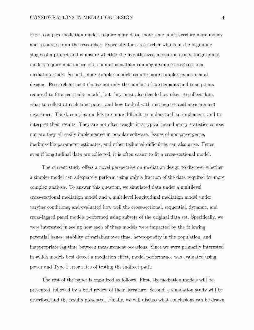
First, complex mediation models require more data, more time, and therefore more money

and resources from the researcher. Especially for a researcher who is in the beginning

stages of a project and is unsure whether the hypothesized mediation exists, longitudinal

models require much more of a commitment than running a simple cross-sectional

mediation study. Second, more complex models require more complex experimental

designs. Researchers must choose not only the number of participants and time points

required to fit a particular model, but they must also decide how often to collect data,

what to collect at each time point, and how to deal with missingness and measurement

invariance. Third, complex models are more di�cult to understand, to implement, and to

interpret their results. They are not often taught in a typical introductory statistics course,

nor are they all easily implemented in popular software. Issues of nonconvergence,

inadmissible parameter estimates, and other technical di�culties can also arise. Hence,

even if longitudinal data are collected, it is often easier to fit a cross-sectional model.

The current study o�ers a novel perspective on mediation design to discover whether

a simpler model can adequately perform using only a fraction of the data required for more

complex analysis. To answer this question, we simulated data under a multilevel

cross-sectional mediation model and a multilevel longitudinal mediation model under

varying conditions, and evaluated how well the cross-sectional, sequential, dynamic, and

cross-lagged panel models performed using subsets of the original data set. Specifically, we

were interested in seeing how each of these models were impacted by the following

potential issues: stability of variables over time, heterogeneity in the population, and

inappropriate lag time between measurement occasions. Since we were primarily interested

in which models best detect a mediation e�ect, model performance was evaluated using

power and Type I error rates of testing the indirect path.

The rest of the paper is organized as follows. First, six mediation models will be

presented, followed by a brief review of their literature. Second, a simulation study will be

described and the results presented. Finally, we will discuss what conclusions can be drawn


from this study as well as o�er some discussion for further study.

Model Formulations for Studying Mediation

This study focuses on the following six mediation models: cross-sectional, sequential,

dynamic, cross-lagged panel, multilevel cross-sectional, and multilevel longitudinal. This is

by no means meant to be an exhaustive list of all possible mediation models, just the

models considered here. All of the models evaluated in this project were estimated within

the SEM framework in MPlus. SEM is particularly useful for mediation analysis because it

can test all paths simultaneously, and so the indirect path can be tested in one step. The

dynamic mediation model was fit in MPlus using the Toeplitz method (Hamaker et al.,

2002). All indirect paths were tested using Sobel standard errors. In general, the authors

recommend using bootstrap standard errors for testing mediation. The same bootstrap

procedure couldn’t be used for all six of these models, however, thus Sobel standard errors

were chosen because they can be used consistently throughout this study. The aim of this

study is to compare relative power of the models not absolute power. As such, consistency

across models is more important in this context. Throughout this paper, we make the same

assumptions as Maxwell and Cole (2007): all variables are either collected without

measurement error or are otherwise latent, and all cross-sectional correlations and path

coe�cients between adjacent time points are invariant across time. For simplicity’s sake,

all of the variables have been centered, and so intercepts have been left out of all model

formulations. It is also important to note that the current paper does not attempt to

discuss causality; it is assumed that the order of the causal pathway has already been

established before performing any of these analyses.

Both cross-sectional mediation and multilevel cross-sectional mediation assume that

the mediation is happening instantaneously, or within time of measurement. The four

longitudinal models - sequential, dynamic, cross-lagged panel, and multilevel longitudinal -

evaluate lagged mediation e�ects. Lag refers to the amount of time that transpires between


adjacent measurement occasions, and so lagged e�ects are those that transpire across time

from one measurement occasion to the next. For example, if the lag is specified as one day,

the model assumes X on Day 1 a�ects values of M on Day 2, and M on Day 2 a�ects values

of Y on Day 3.

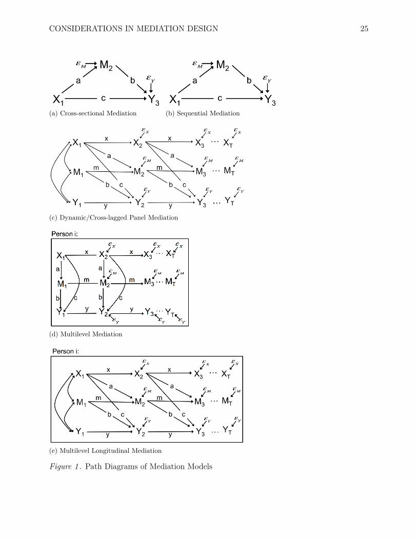
Path diagrams for all of the models are pictured in Figure 1. For all models, a is the

direct path between X and M, b is the direct path between M and Y, and c is the direct

path between X and Y. The direct e�ect describes the e�ect that X has on Y that does not

go through M. The indirect e�ect, or mediation e�ect, describes the e�ect that X has on Y

through M. For all one-level models - cross-sectional, sequential, dynamic, and cross-lagged

panel - the indirect e�ect is calculated by multiplying a and b path coe�cients together,

direct e�ect = c (1)

indirect e�ect = a ◊ b.

The cross-sectional mediation (CSM) model (Figure 1a) is the simplest of the models

presented here. Cross-sectional mediation uses only one measurement occasion, and so

assumes that the cause and e�ect are happening within the time of data collection and are

not impacted by previous realizations of any of the variables involved. The sequential

mediation (SM) model (Figure 1b), originally referred to as the MacArthur approach

(Kraemer et al., 2008), requires that the data are collected in a particular sequence. Like

the CSM model, data for X, M, and Y are each collected only once, but they are collected

longitudinally. X is collected at the first time point, M at the second, and Y at the last

time point. Therefore, this model allows e�ects to take place over time, but still does not

account for previous realizations of the variables.

The remaining models account for previous realizations of the variables through

autoregressive paths. The autoregressive paths of X, M, and Y are labled x, m, and y,


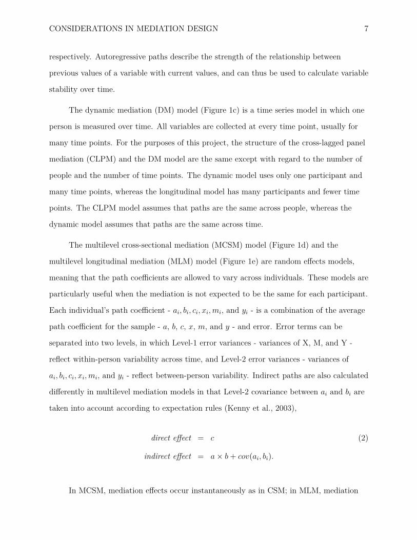
respectively. Autoregressive paths describe the strength of the relationship between

previous values of a variable with current values, and can thus be used to calculate variable

stability over time.

The dynamic mediation (DM) model (Figure 1c) is a time series model in which one

person is measured over time. All variables are collected at every time point, usually for

many time points. For the purposes of this project, the structure of the cross-lagged panel

mediation (CLPM) and the DM model are the same except with regard to the number of

people and the number of time points. The dynamic model uses only one participant and

many time points, whereas the longitudinal model has many participants and fewer time

points. The CLPM model assumes that paths are the same across people, whereas the

dynamic model assumes that paths are the same across time.

The multilevel cross-sectional mediation (MCSM) model (Figure 1d) and the

multilevel longitudinal mediation (MLM) model (Figure 1e) are random e�ects models,

meaning that the path coe�cients are allowed to vary across individuals. These models are

particularly useful when the mediation is not expected to be the same for each participant.

Each individual’s path coe�cient - ai, bi, ci, xi, mi, and yi - is a combination of the average

path coe�cient for the sample - a, b, c, x, m, and y - and error. Error terms can be

separated into two levels, in which Level-1 error variances - variances of X, M, and Y -

reflect within-person variability across time, and Level-2 error variances - variances of

ai, bi, ci, xi, mi, and yi - reflect between-person variability. Indirect paths are also calculated

di�erently in multilevel mediation models in that Level-2 covariance between ai and bi are

taken into account according to expectation rules (Kenny et al., 2003),

direct e�ect = c (2)

indirect e�ect = a ◊ b + cov(ai, bi).

In MCSM, mediation e�ects occur instantaneously as in CSM; in MLM, mediation


e�ects occur over time as in the SM, DM, and CLPM models.

A Brief Review of the Current Models

Although cross-sectional mediation is historically the most popular mediation model,

it has recently been losing favorability in the literature. This is because modeling e�ects

that happen over time in a cross-sectional model almost always produces biased estimates

of both the direct and indirect e�ects. The reason for this bias is two-fold (Gollob &

Reichardt, 1987). First, the cross-sectional model predicts outcomes at the same time

point, not allowing the cause to yet have its e�ect. Second, autoregressive paths are

excluded from the cross-sectional model, necessarily inflating estimates of cross-lagged

paths. Maxwell and Cole (2007) evaluated these biases numerically in a complete

mediation model and found that bias largely depends on the relative stabilities of X and

M, stability being the correlation between a variable with itself at the previous

measurement occasion, flXtXt≠1 . If X and M are equally stable, there is no bias in

estimating the direct path in a cross-sectional model. If X is more stable, the direct path

will be positively biased and if M is more stable it will be negatively biased. Even if X and

M are equally stable, the indirect path will be unbiased if, and only if, one of the following

three conditions hold: (1) a = 0, (2) b = 0, or (3) x

2 = (1 ≠ mx)(1 ≠ xy). Under partial

mediation the amount and direction of bias is more complex, and so the indirect path will

almost always be biased (Maxwell et al., 2011).

Although the sequential mediation model allows for the passage of time between

causes and their e�ects, Mitchell and Maxwell (2013) have found that this model also

su�ers from bias when the underlying model is longitudinal. If autoregressive e�ects are

not controlled, estimation of both the direct and indirect e�ects is biased. Under complete

mediation, sequential mediation sometimes overestimates and sometimes underestimates

the indirect e�ect, but if the stability of X is greater than the stability of M there is

generally less bias. Under partial mediation, the sequential model typically overestimates


the indirect e�ect. As autoregressive paths decrease, bias decreases, as well.

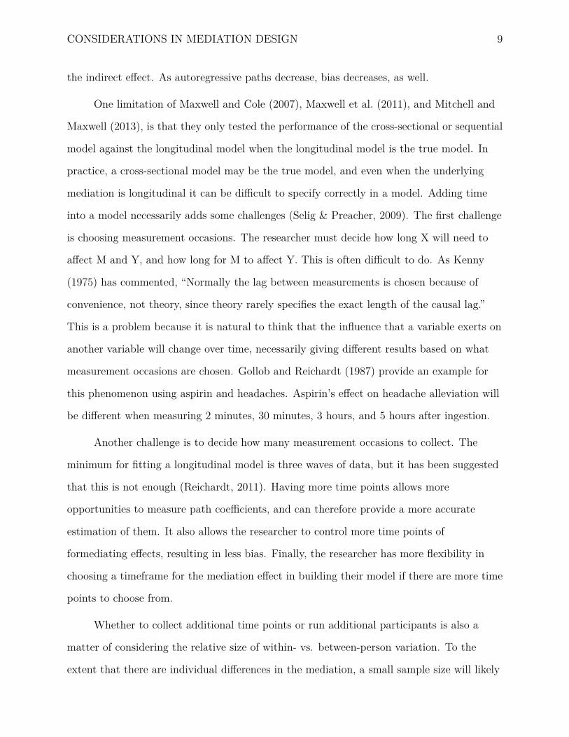
One limitation of Maxwell and Cole (2007), Maxwell et al. (2011), and Mitchell and

Maxwell (2013), is that they only tested the performance of the cross-sectional or sequential

model against the longitudinal model when the longitudinal model is the true model. In

practice, a cross-sectional model may be the true model, and even when the underlying

mediation is longitudinal it can be di�cult to specify correctly in a model. Adding time

into a model necessarily adds some challenges (Selig & Preacher, 2009). The first challenge

is choosing measurement occasions. The researcher must decide how long X will need to

a�ect M and Y, and how long for M to a�ect Y. This is often di�cult to do. As Kenny

(1975) has commented, “Normally the lag between measurements is chosen because of

convenience, not theory, since theory rarely specifies the exact length of the causal lag.”

This is a problem because it is natural to think that the influence that a variable exerts on

another variable will change over time, necessarily giving di�erent results based on what

measurement occasions are chosen. Gollob and Reichardt (1987) provide an example for

this phenomenon using aspirin and headaches. Aspirin’s e�ect on headache alleviation will

be di�erent when measuring 2 minutes, 30 minutes, 3 hours, and 5 hours after ingestion.

Another challenge is to decide how many measurement occasions to collect. The

minimum for fitting a longitudinal model is three waves of data, but it has been suggested

that this is not enough (Reichardt, 2011). Having more time points allows more

opportunities to measure path coe�cients, and can therefore provide a more accurate

estimation of them. It also allows the researcher to control more time points of

formediating e�ects, resulting in less bias. Finally, the researcher has more flexibility in

choosing a timeframe for the mediation e�ect in building their model if there are more time

points to choose from.

Whether to collect additional time points or run additional participants is also a

matter of considering the relative size of within- vs. between-person variation. To the

extent that there are individual di�erences in the mediation, a small sample size will likely


provide biased estimates. Dynamic mediation is an extreme example of this, in which data

is collected on only one individual. Depending on how representative this one person is, the

resulting analysis may or may not be a good representation of the mediation in the

population. On the other hand, if there is more variance within an individual over time

than between individuals, including more time points instead of more people may yield a

more powerful design. All of these considerations - causal lag time, number of

measurement occasions, variable stability, individual di�erences, and others - need to be

explicitly considered when designing a mediation experiment, and so are evaluated in the

following simulation study.

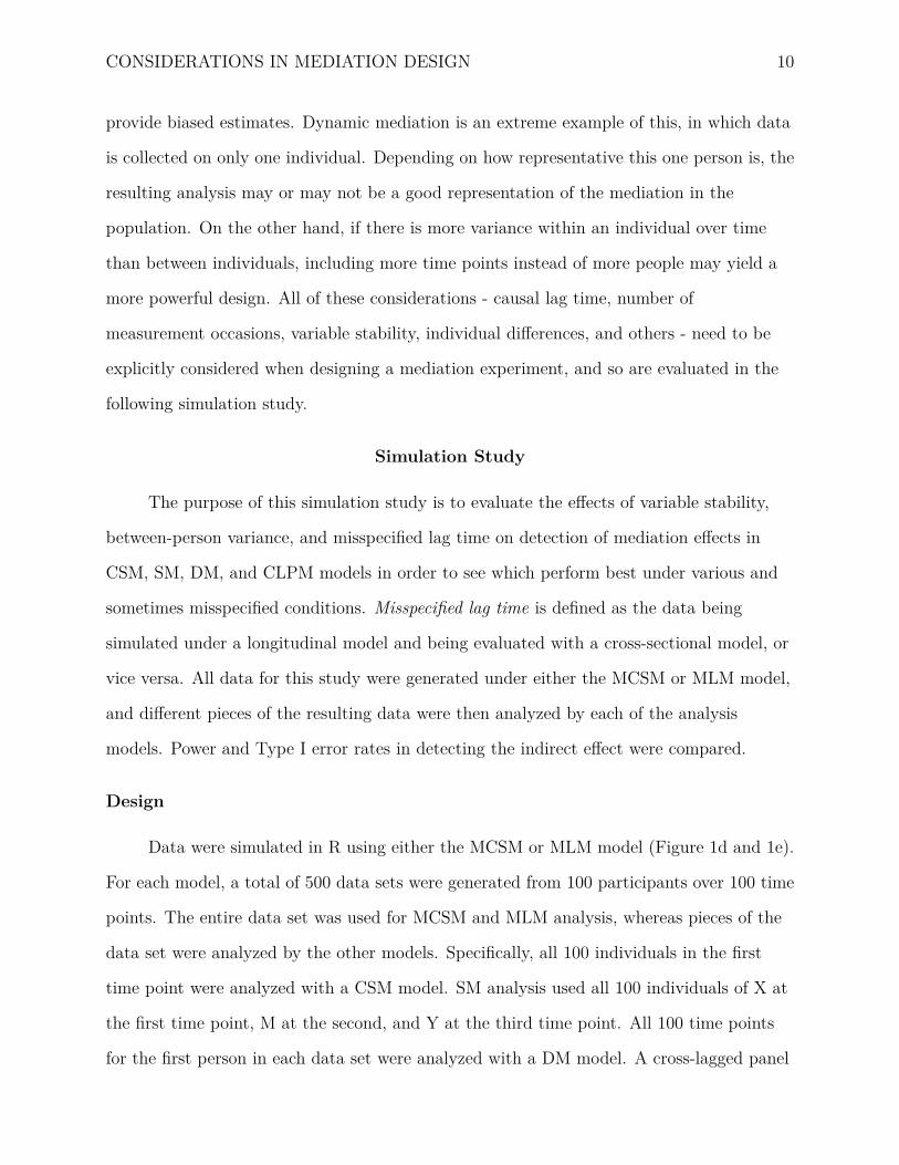
Simulation Study

The purpose of this simulation study is to evaluate the e�ects of variable stability,

between-person variance, and misspecified lag time on detection of mediation e�ects in

CSM, SM, DM, and CLPM models in order to see which perform best under various and

sometimes misspecified conditions. Misspecified lag time is defined as the data being

simulated under a longitudinal model and being evaluated with a cross-sectional model, or

vice versa. All data for this study were generated under either the MCSM or MLM model,

and di�erent pieces of the resulting data were then analyzed by each of the analysis

models. Power and Type I error rates in detecting the indirect e�ect were compared.

Design

Data were simulated in R using either the MCSM or MLM model (Figure 1d and 1e).

For each model, a total of 500 data sets were generated from 100 participants over 100 time

points. The entire data set was used for MCSM and MLM analysis, whereas pieces of the

data set were analyzed by the other models. Specifically, all 100 individuals in the first

time point were analyzed with a CSM model. SM analysis used all 100 individuals of X at

the first time point, M at the second, and Y at the third time point. All 100 time points

for the first person in each data set were analyzed with a DM model. A cross-lagged panel


mediation model was fit using the first 33 people and 3 time points (CLPM3), or the first

20 people and 5 time points (CLPM5). Realistically, lag time for a CLPM model would

likely be longer than that for a DM model. For the purposes of this paper, however, data

for the CLPM models were collected consecutively to keep e�ect sizes similar across models.

In summary, the CSM, SM, DM, CLPM3, and CLPM5 models were each fit to the

same amount of data, 100 data points per variable, from the original data set. MCSM and

MLM models were fit using all 10,000 original data points per variable, 100 times more

data than the aforementioned five models. In fitting all of the longitudinal models, path

coe�cients were constrained to be constant over time. This approach maximizes power

when there is little intraindividual change. The syntax used to analyze each of these

models is available in supplentary material online at www.XXXX.

The path coe�cients, a, b, and c were set to either 0 or 0.36 at all combinations. The

variances of X, M, and Y were set to 1 throughout this study by varying Level-1 error

variance. To quantify the e�ect, Pseudo R-squared and proportion of the e�ect that is

mediated were calculated. Pseudo R-squared was calculated using

Pseudo R

2 = ‡

2‘0 ≠ ‡

2‘1

‡

2‘0

,

where ‡

2‘0 is the population Level-1 error variance for the intercept-only model, and ‡

2‘1 is

the population Level-1 error variance for the model including only that parameter (Singer

& Willett, 2003). Using this formula, an a, b, or c path coe�cient of 0.36 explains about

13% of the variance in the outcome variable, which is generally thought of as a medium

e�ect size using the interpretation of traditional R-squared (Cohen, 1988). The proportion

of the e�ect that is mediated was calculated as

PM = a · b

a · b + c

.

When a = b = c = 0.36, 26.5% of the e�ect of X on Y is being mediated by M (partial


mediation). When either a or b = 0, 0% of the e�ect is being mediated (no mediation), and

when c = 0, 100% of the e�ect is being mediated (complete mediation).

To examine the influence of between-person variability, Level-2 error variance for all

path coe�cients was set to 0, 0.0025, 0.01, or 0.0225 to correspond to standard deviations

in path coe�cients of 0, 0.05, 0.10, and 0.15. Larger values represent more extreme

between-person variability. Throughout this project, all Level-2 error covariances between

path coe�cients were set to 0, i.e. ‡aibi = 0. This may not be the case in empirical data.

For example, individuals with a more stable mediating variable may also be likely to have a

more stable outcome variable, etc., and so setting all covariances to 0 is problematic.

However, there were a couple reasons for making this assumption in the current paper.

First, variances hadn’t yet been evaluated in this context before, and their e�ects should be

established before beginning evaluation of covariances. Second, adding covariances to the

model severely limits other conditions that can be tested while keeping the model

stationary. For these reasons, non-zero covariances were left out of the current project, but

o�er a direction of future research.

To test the influence of X and M stability, X and M were either equally stable

(flXtXt≠1 = flMtMt≠1 = 0.50 or flXtXt≠1 = flMtMt≠1 = 0.36), X was more stable

(flXtXt≠1 = 0.50; flMtMt≠1 = 0.36), or M was more stable (flXtXt≠1 = 0.36; flMtMt≠1 = 0.50).

These correspond to di�erent autoregressive path coe�cients depending on other

conditions. The stability of X is straightforward. In MCSM and MLM, the covariance

between Xt and Xt≠1 is defined as

‡XtXt≠1 = x · ‡

2X ,

where ‡

2X is the variance of X. Because all variances were set to 1 in this simulation, the

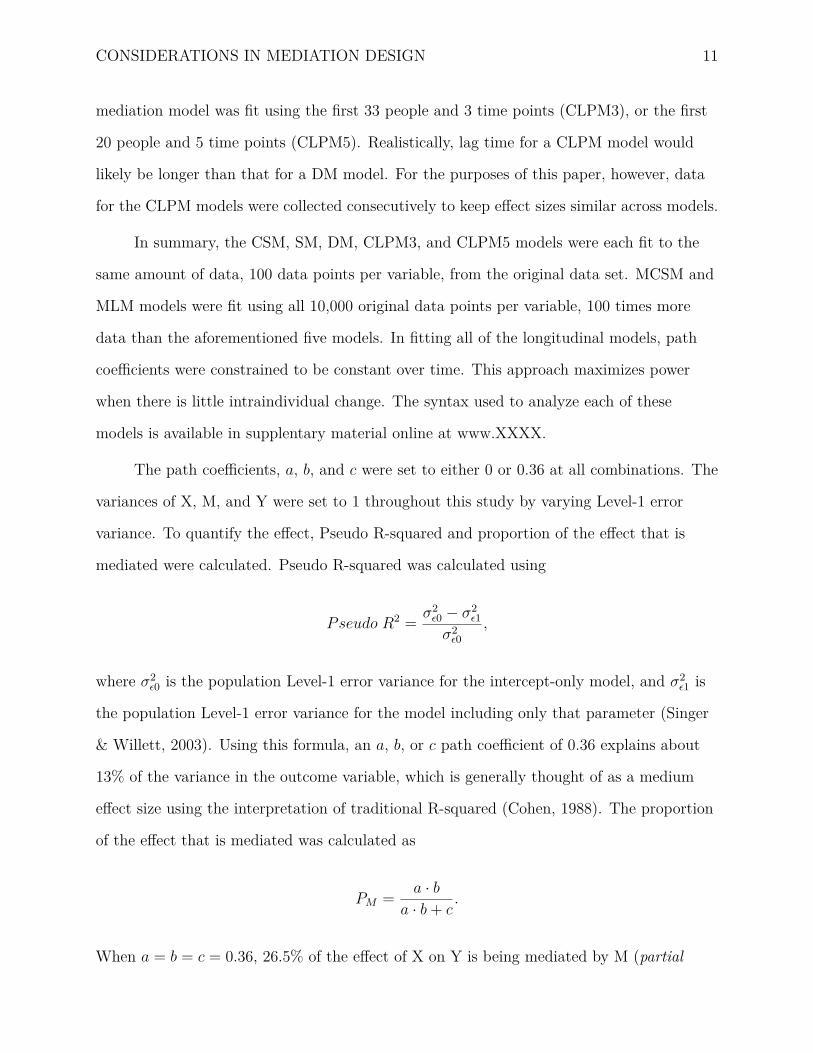
stability of X simplifies to x. The stability of M is a little more complicated. Given the


same simplification of all variances being equal to 1, the stability of M is

flMtMt≠1 = m + a

2x

1 ≠ xm

,

which depends not only on m, but also on x and a. To maintain the stability of M to a

specified level, m paths were varied. For example, to keep the stability of M at 0.50 when

a = .36 and x = .50, m would be set to 0.418. The stability of Y is even more complex but

is not explicitly tested here and so y paths are kept at 0.36 throughout all conditions.

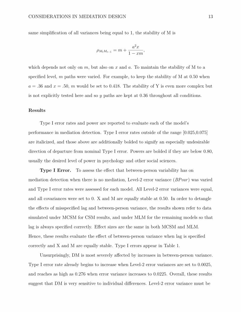
Results

Type I error rates and power are reported to evaluate each of the model’s

performance in mediation detection. Type I error rates outside of the range [0.025,0.075]

are italicized, and those above are additionally bolded to signify an especially undesirable

direction of departure from nominal Type I error. Powers are bolded if they are below 0.80,

usually the desired level of power in psychology and other social sciences.

Type I Error. To assess the e�ect that between-person variability has on

mediation detection when there is no mediation, Level-2 error variance (BPvar) was varied

and Type I error rates were assessed for each model. All Level-2 error variances were equal,

and all covariances were set to 0. X and M are equally stable at 0.50. In order to detangle

the e�ects of misspecified lag and between-person variance, the results shown refer to data

simulated under MCSM for CSM results, and under MLM for the remaining models so that

lag is always specified correctly. E�ect sizes are the same in both MCSM and MLM.

Hence, these results evaluate the e�ect of between-person variance when lag is specified

correctly and X and M are equally stable. Type I errors appear in Table 1.

Unsurprisingly, DM is most severely a�ected by increases in between-person variance.

Type I error rate already begins to increase when Level-2 error variances are set to 0.0025,

and reaches as high as 0.276 when error variance increases to 0.0225. Overall, these results

suggest that DM is very sensitive to individual di�erences. Level-2 error variance must be


less than 0.0025, a standard deviation of 0.05, for DM analysis to be appropriate. CSM

and SM each have one instance of increased Type I error when error variance is 0.0225.

However, these are only slight violations that happen at the most extreme level of

between-person variance.

To assess the e�ect that X and M stability have on mediation detection when there is

no mediation, stability of X and M were set to all combinations of 0.36 and 0.50 and Type

I error rates were assessed for each model. All Level-2 error variances and covariances were

set to 0. When lag is specified correctly, or when lag is specified incorrectly under complete

mediation, all Type I error rates are < 0.05, and so these results are not shown. Results

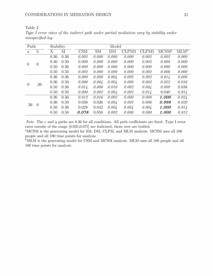
when lag is misspecified under partial mediation are shown in Table 2. Lag is misspecified

when data are simulated under MLM and analyzed with CSM and MCSM, or simulated

under MCSM and analyzed with SM, DM, CLPM, or MLM. Hence, these results evaluate

the e�ect of X and M stability when lag is misspecified without between-person variability.

When a and c are nonzero, MCSM has extremely high Type I error rates. These

results show that when the lag is unknown, MCSM should not be utilized. CSM has one

slight violation in these conditions, as well, which appears to increase as stability of X and

M increase.

Power. To assess the e�ect that between-person variability has on detecting a true

mediation, Level-2 error variance was varied and power rates were assessed for each model.

Again, these results address what is the e�ect of between-person variance when lag is

specified correctly and X and M are equally stable at 0.50. All results are shown in Table

3. Across conditions, CSM and SM are the most powerful among the one-level models and

seem to be una�ected by between-person variance. DM is most a�ected by increases in

between-person variance. Under partial mediation, power decreases from 0.99 with no

between-person variance to 0.79 at the most extreme variance. Nonetheless, DM is still

more powerful than CLPM3 under most conditions.

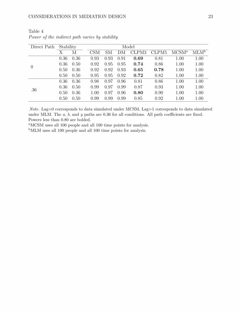
To assess the e�ect that X and M stability have on detecting a true mediation,


stability of X and M were set to all combinations of 0.36 and 0.50 and power rates were

assessed for each model. All Level-2 error variances and covariances were set to 0. Results

under correctly specified lag are shown in Table 4, and under misspecified lag in Table 5.

Higher stability increases power insubstantially when lag is correctly specified, whereas the

impact under misspecified lag is severe.

As expected, overall power is much lower under misspecified lag. The multilevel

models are the only models to have similar power rates as they did under correctly

specified lag. The model that performs next best is SM. SM power reaches as high as 64%

when the stability of both X and M are at their highest, 0.50, and when the direct path is

nonzero. Performance quickly drops with decreases in X and especially M stability, as well

as when the direct path becomes 0. The next highest power reported is that by CSM,

reaching as high as 48%, but quickly dropping under the same conditions. DM and CLPM

models never have power higher than 11%, and most rates are much lower than that.

Conclusions. Type I error rates are well contained throughout this study with a

couple of exceptions. DM was sensitive to increases in between-person variance, and

MCSM performed poorly under misspecified lag. Overall, Type I error rates were much

lower than the nominal 0.05 when both a=0 and b=0, but these results agree with those by

MacKinnon et al. (2002) when the Sobel test is utilized.

Apart from the multilevel models, CSM and SM had the highest power, followed by

DM, CLPM5 and CLPM3 had the lowest power. The power of DM was most a�ected by

increases in between-person variance, and all models were mildly a�ected by increases in X

and M stability. Most interesting are the power rates under misspecified lag. Apart from

the multilevel models, CSM and especially SM performed the best in these conditions.

Discussion

The goal of the current project was to determine whether a simpler mediation model

that utilizes less data can perform as well as a more complex model in detecting a


mediation e�ect. Models were evaluated and compared under conditions of alternative

variable stabilities, between-person variation, and misspecified lag. Relative stabilities of X

and M variables did not a�ect either Type I error rate or power by notable amounts,

except in the case when lag was misspecified. Models performed much better under

misspecified lags with higher stability variables, especially SM and CSM. Between-person

variance most a�ected DM in terms of both Type I error rate and power. In all conditions,

simulations showed that detecting a mediation e�ect under partial mediation was more

powerful than under complete mediation.

The multilevel models had the highest power in all conditions, but they also used 100

times more data than the other models. MCSM had very high Type I error rates when lag

was misspecified, but MLM never had a higher than nominal Type-1 error rate. Thus, if

resources allow, the results of this paper highly recommend MLM as the superior model to

evaluate mediation. Even in misspecified conditions, the MLM performed well. This is

especially an advantage in mediation, when the researcher may not know whether the e�ect

is cross-sectional or longitudinal or what the correct lag may be. As long as enough data

points are collected, the MLM model can be trusted to provide an accurate result.

Of the remaining models, CSM and SM models were the next most powerful, with

DM shortly thereafter. A CLPM with 5 time points and 20 people was always more

powerful than a CLPM with 3 time points and 33 people, further supporting Reichardt’s

(2011) argument that three waves are not enough. The CLPM models are the only two

models to maintain Type-1 error in all conditions. SM and CSM were the only models to

capture the mediation e�ect when the lag was misspecified. Although these results highly

depend on the stability of X and M, their performances are still impressive considering that

0.089 is the highest Type I error rate from either of these models. Therefore, if resources

do not allow for MLM analysis and the stabilities of X and M are expected to be high, SM

is a viable alternative to MLM.

These results may be surprising to some readers who have read previous work


comparing CSM and SM to longitudinal models such as Maxwell and Cole (2007), Maxwell

et al. (2011), and Mitchell and Maxwell (2013), but these papers focused on bias. It very

well may be that CSM and SM were so powerful in some of these conditions due to bias.

Regardless, as long as Type I error is not inflated, bias would not pose a practical problem

if the goal is to detect a mediation e�ect. That being said, this paper is in no way meant to

discourage focus on e�ect sizes in the literature. We still believe e�ect size estimation is an

important part of the research process. However, calculation of e�ect size for longitudinal

models, especially longitudinal mediation models is a complex issue (Peugh, 2010; Roberts

& Monaco, 2006; Preacher & Kelley, 2011). As such, many researchers rely more on power

than e�ect size in evaluating complex models such as some of the models presented here.

On the contrary, it is well-known that CSM and SM can be biased (i.e. Mitchell &

Maxwell, 2013), thus their results should always be hesitantly interpreted.

Despite these limitations, this paper serves as a fundamental first step in evaluating

mediation models from the perspective of an empirical researcher interested in detecting a

mediation e�ect. It is our goal that the methods utilized here set the stage for future

projects from this perspective, and encourage future quantitative work in mediation that

will be most useful to its users. This perspective has not been explored before, and so

o�ers some new results. When ample time and resources are available, or the researcher

desires to investigate more complex phenomena, these results highly recommend the use of

a multilevel longitudinal mediation model. It has high power to find a mediation e�ect and

still maintain Type I error rate even under misspecified lag. When multilevel longitudinal

mediation analysis is not possible or desirable, the results of this paper suggest utilization

of cross-sectional and especially sequential mediation. Accordingly, we recommend

sequential mediation models as a low-cost option for researchers seeking to maximize power

using minimal resources.


References

Baron, R. M., & Kenny, D. A. (1986). The moderatorâmediator variable distinction in

social psychological research: Conceptual, strategic, and statistical considerations.

Journal of personality and social psychology, 51 (6), 1173.

Cohen, J. (1988). Statistical power analysis for the behavioral sciences (2nd ed.). Lawrence

Erlbaum Associates.

Gollob, H. F., & Reichardt, C. S. (1987, February). Taking Account of Time Lags in

Causal Models. Child Development, 58 (1), 80. doi: 10.2307/1130293

Hamaker, E. L., Dolan, C. V., & Molenaar, P. C. M. (2002, July). On the Nature of SEM

Estimates of ARMA Parameters. Structural Equation Modeling: A Multidisciplinary

Journal, 9 (3), 347–368. doi: 10.1207/S15328007SEM0903_3

Kenny, D. A. (1975). Cross-lagged panel correlation: A test for spuriousness. Psychological

Bulletin, 82 (6), 887. doi: 10.1037/0033-2909.82.6.887

Kenny, D. A., Korchmaros, J. D., & Bolger, N. (2003). Lower level mediation in multilevel

models. Psychological Methods, 8 (2), 115–128. doi: 10.1037/1082-989X.8.2.115

Kraemer, H. C., Kiernan, M., Essex, M., & Kupfer, D. J. (2008). How and why criteria

defining moderators and mediators di�er between the Baron & Kenny and MacArthur

approaches. Health Psychology, 27 (2, Suppl), S101–S108. doi:

10.1037/0278-6133.27.2(Suppl.).S101

MacKinnon, D. P., Lockwood, C. M., Ho�man, J. M., West, S. G., & Sheets, V. (2002). A

comparison of methods to test mediation and other intervening variable e�ects.

Psychological methods, 7 (1), 83.

Maxwell, S. E., & Cole, D. A. (2007). Bias in cross-sectional analyses of longitudinal

mediation. Psychological Methods, 12 (1), 23–44. doi: 10.1037/1082-989X.12.1.23


Maxwell, S. E., Cole, D. A., & Mitchell, M. A. (2011, September). Bias in Cross-Sectional

Analyses of Longitudinal Mediation: Partial and Complete Mediation Under an

Autoregressive Model. Multivariate Behavioral Research, 46 (5), 816–841. doi:

10.1080/00273171.2011.606716

Mitchell, M. A., & Maxwell, S. E. (2013, May). A Comparison of the Cross-Sectional and

Sequential Designs when Assessing Longitudinal Mediation. Multivariate Behavioral

Research, 48 (3), 301–339. doi: 10.1080/00273171.2013.784696

Peugh, J. L. (2010, February). A practical guide to multilevel modeling. Journal of School

Psychology, 48 (1), 85–112. doi: 10.1016/j.jsp.2009.09.002

Preacher, K. J., & Kelley, K. (2011). E�ect size measures for mediation models:

Quantitative strategies for communicating indirect e�ects. Psychological Methods, 16 (2),

93–115. doi: 10.1037/a0022658

Reichardt, C. S. (2011, September). Commentary: Are Three Waves of Data Su�cient for

Assessing Mediation? Multivariate Behavioral Research, 46 (5), 842–851. doi:

10.1080/00273171.2011.606740

Roberts, J., & Monaco, J. P. (2006). E�ect size measures for the two-level linear multilevel

model. In annual meeting of the American Educational Research Association, San

Francisco, CA.

Selig, J. P., & Preacher, K. J. (2009, June). Mediation Models for Longitudinal Data in

Developmental Research. Research in Human Development, 6 (2-3), 144–164. doi:

10.1080/15427600902911247

Singer, J. D., & Willett, J. B. (2003). Applied longitudinal data analysis: Modeling change

and event occurrence. Oxford university press.


Table 1Type I error rates of the indirect path vary by between-person variance

Path Modela b c BPvar CSM SM DM CLPM3 CLPM5 MCSMa MLMb

0 0 0

0 0.000 0.000 0.002 0.000 0.000 0.000 0.0000.0025 0.000 0.000 0.000 0.002 0.002 0.028 0.0080.01 0.002 0.000 0.020 0.000 0.002 0.050 0.0600.0225 0.002 0.006 0.058 0.004 0.002 0.047 0.067

0 .36 0

0 0.034 0.042 0.036 0.022 0.044 0.044 0.0280.0025 0.040 0.034 0.070 0.036 0.046 0.046 0.0400.01 0.026 0.030 0.126 0.022 0.052 0.056 0.0580.0225 0.069 0.089 0.240 0.048 0.058 0.052 0.054

.36 0 0

0 0.030 0.044 0.032 0.024 0.042 0.070 0.0320.0025 0.048 0.038 0.074 0.012 0.066 0.054 0.0600.01 0.038 0.032 0.114 0.036 0.028 0.050 0.0540.0225 0.036 0.036 0.192 0.040 0.058 0.047 0.039

0 0 .36

0 0.000 0.000 0.000 0.000 0.000 0.000 0.0000.0025 0.000 0.000 0.004 0.000 0.000 0.032 0.0280.01 0.000 0.000 0.016 0.002 0.000 0.048 0.0500.0225 0.010 0.000 0.062 0.002 0.004 0.047 0.046

0 .36 .36

0 0.036 0.032 0.020 0.032 0.032 0.048 0.0280.0025 0.042 0.010 0.088 0.020 0.064 0.050 0.0500.01 0.042 0.044 0.166 0.048 0.070 0.072 0.0540.0225 0.089 0.075 0.267 0.053 0.075 0.052 0.064

.36 0 .36

0 0.026 0.054 0.040 0.038 0.058 0.066 0.0300.0025 0.042 0.034 0.058 0.042 0.050 0.042 0.0640.01 0.030 0.034 0.116 0.028 0.048 0.070 0.0780.0225 0.054 0.044 0.275 0.037 0.051 0.067 0.043

Note. X and M are equally stable at 0.50, the y path is 0.36 for all conditions. All path coe�cients

are fixed. Type I error rates outside of the range [0.025,0.075] are italicized, those over are bolded.

aMCSM is the generating model for MCSM and CSM analysis. MCSM uses all 100 people and all

100 time points for analysis.

bMLM is the generating model for MLM, SM, DM, and CLPM analysis. MLM uses all 100 people

and all 100 time points for analysis.


Table 2Type I error rates of the indirect path under partial mediation vary by stability undermisspecified lag

Path Stability Modela b X M CSM SM DM CLPM3 CLPM5 MCSMa MLMb

0 0

0.36 0.36 0.002 0.000 0.000 0.000 0.002 0.002 0.0000.36 0.50 0.000 0.000 0.000 0.000 0.002 0.008 0.0000.50 0.36 0.000 0.000 0.000 0.000 0.000 0.000 0.0000.50 0.50 0.002 0.000 0.000 0.000 0.002 0.006 0.000

0 .36

0.36 0.36 0.000 0.000 0.004 0.002 0.002 0.014 0.0060.36 0.50 0.000 0.004 0.004 0.008 0.002 0.022 0.0160.50 0.36 0.014 0.006 0.010 0.002 0.004 0.008 0.0380.50 0.50 0.000 0.002 0.004 0.002 0.014 0.040 0.014

.36 0

0.36 0.36 0.012 0.016 0.002 0.000 0.008 1.000 0.0240.36 0.50 0.038 0.026 0.004 0.002 0.006 0.998 0.0200.50 0.36 0.028 0.042 0.004 0.004 0.004 1.000 0.0140.50 0.50 0.078 0.050 0.002 0.006 0.000 1.000 0.012

Note. The c and y paths are 0.36 for all conditions. All path coe�cients are fixed. Type I error

rates outside of the range [0.025,0.075] are italicized, those over are bolded.

aMCSM is the generating model for SM, DM, CLPM, and MLM analysis. MCSM uses all 100

people and all 100 time points for analysis.

bMLM is the generating model for CSM and MCSM analysis. MLM uses all 100 people and all



Table 3Power in detecting the indirect path varies by between-person variance

ModelDirect Path BPvar CSM SM DM CLPM3 CLPM5 MCSMa MLMb

0

0 0.95 0.95 0.92 0.72 0.82 1.00 1.000.0025 0.95 0.94 0.90 0.72 0.83 1.00 1.000.01 0.96 0.96 0.79 0.76 0.81 1.00 1.000.0225 0.95 0.97 0.74 0.69 0.81 1.00 1.00

.36

0 0.99 0.99 0.99 0.85 0.92 1.00 1.000.0025 1.00 0.99 0.95 0.85 0.90 1.00 1.000.01 1.00 0.99 0.89 0.85 0.89 1.00 1.000.0225 0.99 0.99 0.79 0.86 0.88 1.00 1.00

Note. X and M are equally stable at 0.50 and the a, b and y paths are 0.36 for all conditions. All

path coe�cients are fixed. Powers less than 0.80 are bolded.

aMCSM is the generating model for MCSM and CSM analysis. MCSM uses all 100 people and all


bMLM is the generating model for MLM, SM, DM, and CLPM analysis. MLM uses all 100 people

and all 100 time points for analysis.


Table 4Power of the indirect path varies by stability

Direct Path Stability ModelX M CSM SM DM CLPM3 CLPM5 MCSMa MLMb

0

0.36 0.36 0.93 0.93 0.91 0.69 0.81 1.00 1.000.36 0.50 0.92 0.95 0.95 0.74 0.86 1.00 1.000.50 0.36 0.92 0.92 0.93 0.65 0.78 1.00 1.000.50 0.50 0.95 0.95 0.92 0.72 0.82 1.00 1.00

.36

0.36 0.36 0.98 0.97 0.96 0.81 0.86 1.00 1.000.36 0.50 0.99 0.97 0.99 0.87 0.93 1.00 1.000.50 0.36 1.00 0.97 0.96 0.80 0.90 1.00 1.000.50 0.50 0.99 0.99 0.99 0.85 0.92 1.00 1.00

Note. Lag=0 corresponds to data simulated under MCSM, Lag=1 corresponds to data simulated

under MLM. The a, b, and y paths are 0.36 for all conditions. All path coe�cients are fixed.

Powers less than 0.80 are bolded.

aMCSM uses all 100 people and all 100 time points for analysis.

bMLM uses all 100 people and all 100 time points for analysis.


Table 5Power of the indirect path varies by stability under misspecified lag

Direct Path Stability ModelX M CSM SM DM CLPM3 CLPM5 MCSMa MLMb

0

0.36 0.36 0.02 0.10 0.00 0.01 0.02 0.99 1.000.36 0.50 0.05 0.10 0.01 0.02 0.01 1.00 0.980.50 0.36 0.05 0.29 0.03 0.03 0.04 0.99 1.000.50 0.50 0.12 0.27 0.05 0.03 0.04 1.00 0.99

.36

0.36 0.36 0.15 0.19 0.02 0.02 0.01 0.99 0.990.36 0.50 0.28 0.25 0.04 0.01 0.03 0.99 1.000.50 0.36 0.20 0.49 0.06 0.02 0.02 0.97 1.000.50 0.50 0.48 0.64 0.11 0.04 0.05 0.99 1.00

Note. Lag=0 corresponds to data simulated under MCSM, Lag=1 corresponds to data simulated

under MLM. The a, b, and y paths are 0.36 for all conditions. All path coe�cients are fixed.

Powers less than 0.80 are bolded.

aMCSM uses all 100 people and all 100 time points for analysis.

bMLM uses all 100 people and all 100 time points for analysis.


(a) Cross-sectional Mediation (b) Sequential Mediation

(c) Dynamic/Cross-lagged Panel Mediation

(d) Multilevel Mediation

(e) Multilevel Longitudinal Mediation

Figure 1 . Path Diagrams of Mediation Models

Documents

Time and Other Considerations in Mediation Design Meghan K