Embed Size (px)
Citation preview

Guixia Kang
Nibelungenstr. 50
Munchen, Deutschland
Time and frequency domain joint channel estimation
in multi-carrier multi-branch systems
deutscher Titel:
Gemeinsame Kanalschatzung im Zeit- und Frequenzbereich
fur Mehrtragerubertragungsverfahren mit mehreren
Ubertragungszweigen
Vom Fachbereich Elektrotechnik und Informationstechnik
der Technischen Universitat Kaiserslautern
zur Verleihung des akademischen Grades
Doktor der Ingenieurwissenschaften (Dr.–Ing.)
genehmigte Dissertation
von
Dr.–Eng. Guixia Kang
D 386
Tag der Einreichung: 27. Oktober 2004Tag der mundlichen Prufung: 18. Februar 2005
Dekan des Fachbereichs: Prof. Dr.–Ing. G. Huth
Vorsitzender derPrufungskommission: Prof. Dr.–Ing. R. Urbansky
1. Berichterstatter: Prof. Dr.–Ing. habil. Dr.-Ing. E. h. P. W. Baier2. Berichterstatter: Prof. Dr.–Ing. habil. J. Gotze


I
Preface
The available work is developed from Oct 2002 to Oct 2004 in line with my activity as ascientific researcher in the Future Radio department of ICM (Information CommunicationMobile) of Siemens AG in Munich, Germany. I would like to thank all who have supportedme on the accomplishment of this work.
My special appreciation is given to Mr. Prof. Dr.–Ing. habil. Dr.–Ing. E.h. P. W. Baier,the director of the Research Group for RF communications of the University of Kaisers-lautern, for the many valuable suggestions and the support to my work. His constantreadiness for discussion as well as the numerous proper references he gave me improvedthis work substantially.
My friends and colleagues in Siemens are appreciated for providing the pleasant atmo-sphere of academic exchange for the promotion of my work. Particularly, I would liketo thank Dr.–Ing. E. Schulz for providing the necessary facilities and conditions for theresearch and Mr. Dr.–Ing. M. Weckerle for his concrete suggestions and discussions andreview of my thesis work. With their help, my theoretical work was put into the contextof some future wireless system concepts in the project of JRB3G (Joint Research Beyond3G) for verification. Dr.–Ing. E. Costa, Mr. J. Eichinger, and Mr. A. Filippi are alsothanked for the valuable discussions, and Mr. R. Halfmann is thanked for making thecomputer and software run effectively.
I thank also my friends in the the Research Group for RF communications of the Universityof Kaiserslautern for the fruitful discussions. Special thanks are given to Dr.–Ing. habil. T.Weber and Mr. I. Maniatis for the discussions on the joint channel estimation techniques,as well as to Mrs. Y. Liu for providing some simulation chains and for the discussion onthe simulation tools and parameters.
My genuine appreciation is given also to Mr. Prof. Dr.–Ing. P. Zhang of Beijing Universityof Posts and Telecommunications, who has guided me into the fancy world of wirelesscommunications.
I cordially thank to my family, in particular my parents, who made my education andtraining possible and always support me. Finally I thank my husband, Dr.–Ing. D. Liu,who gave me in this time a crucial support. I would like to dedicate this work to them.
Munich, October 2004 Guixia Kang

CONTENTS III
Contents
1 Introduction 1
1.1 JCE in the uplink of synchronous mobile wireless systems . . . . . . . . . . 1
1.1.1 General . . . . . . . . . . . . . . . . . . . . . . . . . . . . . . . . . 1
1.1.2 Application scenarios of JCE . . . . . . . . . . . . . . . . . . . . . . 3
1.1.3 Time and frequency domain JCE . . . . . . . . . . . . . . . . . . . 6
1.1.4 State of the art in JCE techniques . . . . . . . . . . . . . . . . . . . 7
1.2 Multi-branch systems . . . . . . . . . . . . . . . . . . . . . . . . . . . . . . 8
1.3 Pilots for JCE . . . . . . . . . . . . . . . . . . . . . . . . . . . . . . . . . . 11
1.3.1 General . . . . . . . . . . . . . . . . . . . . . . . . . . . . . . . . . 11
1.3.2 State of the art in pilot design for JCE . . . . . . . . . . . . . . . . 12
1.4 Goals of this thesis . . . . . . . . . . . . . . . . . . . . . . . . . . . . . . . 13
1.5 Contents and important results . . . . . . . . . . . . . . . . . . . . . . . . 14
2 Mobile radio channel model 17
2.1 Introduction . . . . . . . . . . . . . . . . . . . . . . . . . . . . . . . . . . . 17
2.2 WSSUS broadband channel model . . . . . . . . . . . . . . . . . . . . . . . 19
2.2.1 Broadband channel characterization . . . . . . . . . . . . . . . . . . 19
2.2.2 Stochastic channel description . . . . . . . . . . . . . . . . . . . . . 20
2.3 Beyond 3G channel . . . . . . . . . . . . . . . . . . . . . . . . . . . . . . . 24
2.3.1 Channel parameters . . . . . . . . . . . . . . . . . . . . . . . . . . 24
2.3.2 Channel simulations . . . . . . . . . . . . . . . . . . . . . . . . . . 25
2.4 Multi-branch channel consideration . . . . . . . . . . . . . . . . . . . . . . 26
2.5 Interference model . . . . . . . . . . . . . . . . . . . . . . . . . . . . . . . 29
3 JCE in multi-branch systems 31
3.1 Introduction . . . . . . . . . . . . . . . . . . . . . . . . . . . . . . . . . . . 31
3.2 Description of the problems of JCE . . . . . . . . . . . . . . . . . . . . . . 32
3.3 Frequency domain representation of JCE . . . . . . . . . . . . . . . . . . . 36
3.3.1 Discrete frequency model . . . . . . . . . . . . . . . . . . . . . . . . 36
3.3.2 FD-JCE algorithms . . . . . . . . . . . . . . . . . . . . . . . . . . . 41
3.3.3 SNR degradation . . . . . . . . . . . . . . . . . . . . . . . . . . . . 43
3.3.4 MSE . . . . . . . . . . . . . . . . . . . . . . . . . . . . . . . . . . . 45
3.3.5 Variation coefficient . . . . . . . . . . . . . . . . . . . . . . . . . . . 47
3.4 Time domain representation of JCE . . . . . . . . . . . . . . . . . . . . . . 48
3.4.1 Introduction . . . . . . . . . . . . . . . . . . . . . . . . . . . . . . . 48
3.4.2 The shift property of DFT . . . . . . . . . . . . . . . . . . . . . . . 48
3.4.3 Discrete time model . . . . . . . . . . . . . . . . . . . . . . . . . . 50
3.4.4 TD-JCE . . . . . . . . . . . . . . . . . . . . . . . . . . . . . . . . . 53
3.4.5 SNR degradation . . . . . . . . . . . . . . . . . . . . . . . . . . . . 54
3.4.6 MSE . . . . . . . . . . . . . . . . . . . . . . . . . . . . . . . . . . . 55

IV CONTENTS
3.5 List of estimators . . . . . . . . . . . . . . . . . . . . . . . . . . . . . . . . 55
4 Optimum and suboptimum pilots for JCE in noise limited systems 57
4.1 Introduction . . . . . . . . . . . . . . . . . . . . . . . . . . . . . . . . . . . 57
4.2 Design criteria of optimum pilots . . . . . . . . . . . . . . . . . . . . . . . 58
4.2.1 Frequency domain . . . . . . . . . . . . . . . . . . . . . . . . . . . 58
4.2.2 Time domain . . . . . . . . . . . . . . . . . . . . . . . . . . . . . . 61
4.2.3 Equivalence between the time and frequency domain design criteria
of optimum pilots . . . . . . . . . . . . . . . . . . . . . . . . . . . . 63
4.3 Optimum pilots . . . . . . . . . . . . . . . . . . . . . . . . . . . . . . . . . 64
4.3.1 Introduction . . . . . . . . . . . . . . . . . . . . . . . . . . . . . . . 64
4.3.2 Disjoint pilots . . . . . . . . . . . . . . . . . . . . . . . . . . . . . . 64
4.3.3 Walsh code based pilots . . . . . . . . . . . . . . . . . . . . . . . . 65
4.3.4 CAZAC code based pilots . . . . . . . . . . . . . . . . . . . . . . . 67
4.3.5 Proof of the optimum pilots . . . . . . . . . . . . . . . . . . . . . . 71
4.4 Suboptimum pilots . . . . . . . . . . . . . . . . . . . . . . . . . . . . . . . 72
4.5 Numerical results of SNR degradations . . . . . . . . . . . . . . . . . . . . 73
5 Pilot assignment in multiple SA environments 76
5.1 Introduction . . . . . . . . . . . . . . . . . . . . . . . . . . . . . . . . . . . 76
5.2 Pilot assignment problem in interference environments . . . . . . . . . . . 77
5.3 Variation coefficient simulation . . . . . . . . . . . . . . . . . . . . . . . . 79
5.4 Proposals of pilot assignment for multiple SAs . . . . . . . . . . . . . . . . 85
6 Application of JCE in OFDM and FMT based multi-branch systems 88
6.1 Introduction . . . . . . . . . . . . . . . . . . . . . . . . . . . . . . . . . . . 88
6.2 Multi-carrier systems . . . . . . . . . . . . . . . . . . . . . . . . . . . . . . 88
6.2.1 Introduction . . . . . . . . . . . . . . . . . . . . . . . . . . . . . . . 88
6.2.2 FB-MC modulation . . . . . . . . . . . . . . . . . . . . . . . . . . . 89
6.2.3 OFDM modulation . . . . . . . . . . . . . . . . . . . . . . . . . . . 90
6.2.4 FMT modulation . . . . . . . . . . . . . . . . . . . . . . . . . . . . 92
6.3 Time versus frequency domain JCE for OFDM and FMT systems . . . . . 94
6.4 PAPR issue in OFDM systems . . . . . . . . . . . . . . . . . . . . . . . . . 98
6.4.1 General . . . . . . . . . . . . . . . . . . . . . . . . . . . . . . . . . 98
6.4.2 PAPR comparison of various pilots . . . . . . . . . . . . . . . . . . 99
6.5 Applications of various optimum pilots . . . . . . . . . . . . . . . . . . . . 101
7 Simulations of JCE in OFDM and FMT based multi-branch systems 102
7.1 General . . . . . . . . . . . . . . . . . . . . . . . . . . . . . . . . . . . . . 102
7.2 Simulation scenarios . . . . . . . . . . . . . . . . . . . . . . . . . . . . . . 102
7.2.1 OFDM simulation parameters . . . . . . . . . . . . . . . . . . . . . 102
7.2.2 FMT simulation parameters . . . . . . . . . . . . . . . . . . . . . . 104
7.2.3 Definition of SNR . . . . . . . . . . . . . . . . . . . . . . . . . . . . 106

CONTENTS V
7.3 Performance of JCE in the multi-branch OFDM system . . . . . . . . . . . 107
7.3.1 Subchannel simulation . . . . . . . . . . . . . . . . . . . . . . . . . 107
7.3.2 MSE simulation . . . . . . . . . . . . . . . . . . . . . . . . . . . . . 109
7.3.3 BER simulation . . . . . . . . . . . . . . . . . . . . . . . . . . . . . 114
7.4 Performance of JCE in multi-branch FMT systems . . . . . . . . . . . . . 119
7.4.1 Subchannel simulation . . . . . . . . . . . . . . . . . . . . . . . . . 119
7.4.2 MSE simulation . . . . . . . . . . . . . . . . . . . . . . . . . . . . . 120
7.4.3 BER simulation . . . . . . . . . . . . . . . . . . . . . . . . . . . . . 125
8 Summary 130
8.1 English . . . . . . . . . . . . . . . . . . . . . . . . . . . . . . . . . . . . . . 130
8.2 German . . . . . . . . . . . . . . . . . . . . . . . . . . . . . . . . . . . . . 131
Appendix 133
A.1 Abbreviations . . . . . . . . . . . . . . . . . . . . . . . . . . . . . . . . . . 133
A.2 Symbols . . . . . . . . . . . . . . . . . . . . . . . . . . . . . . . . . . . . . 134
References 140


1
1 Introduction
1.1 JCE in the uplink of synchronous mobile wireless
systems
1.1.1 General
Recently, wireless communication systems are developing from the third generation (3G)
into the beyond 3G or fourth generation (4G) due to the increasing demands of mobile
user data services. In order to maximize the profit of the investment by the system
operators on the scarce and, therefore, valuable spectrum resource, the beyond 3G sys-
tems will support high data rate services with higher spectral efficiency than previous
systems over broadband channels [BBT02, BaM02, CS00, KJC+03]. Furthermore, the
operators of the wireless communication systems expect to support more users transmit-
ting simultaneously with acceptable quality of service (QoS) over the limited resource.
Consequently, the system designers have to face the challenge of achieving higher system
capacity. The important factor that limits the system capacity in multi-user simulta-
neous transmission is the multiple access interference (MAI) [Ver98]. In the broadband
channels, the MAI problem becomes even worse because each user may produce multiple
replicas of the transmitted signal at the receiver due to the frequency selectivity of the
channel [Pro95, Rap96]. Various possibilities to mitigate or even cancel MAI are under in-
vestigation, such as the interference cancellation (IC) techniques [EGL93, KIH87] and joint
detection (JD) [Ver98, SWB02] at the receiver and joint transmission (JT) [BMW+00]
at the transmitter. In these approaches, the knowledge of the radio channels of these
multiple active users, either their transfer functions (TF) or their channel impulse re-
sponses (CIR), is presupposed. One widely used method to estimate the radio channels
is to periodically transmit training signals which are a-priori known to the receiver. The
channel knowledge is achieved based on the received training signals caused by the trans-
mitted training signals. The training signals, during the multi-user transmission process
over the frequency selective channels, will also incur MAI like problems at the receiver.
Therefore, it is necessary to introduce a MAI cancellation like technique into the channel
estimation, and thereby the joint channel estimation (JCE) [SJ94, SMW+01] is derived.
Different from traditional single user channel estimation techniques [Pro95], in JCE not
only the channel knowledge of the considered user but also that of the interferers within
a certain geographic area named cell or service area (SA) are estimated jointly. The well
designed JCE can completely cancel the interference between different users in the channel
estimation process.
In mobile wireless systems using frequency division multiple access (FDMA) and time
division multiple access (TDMA) as for example in the second generation (2G) global

2 Chapter 1: Introduction
system for mobile communications (GSM) [GSM88], channel estimation is a relatively
simple task because the signals of the active users are separated either in time or in fre-
quency. In the asynchronous code division multiple access (CDMA) systems, such as the
2G IS-95 CDMA system [Gar99] and the 3G wideband CDMA (WCDMA) system [HT02],
the signals associated with the active users which are not intended to be detected in the
considered cell are treated as noise, and matched filtering or RAKE receivers [Pro95] are
applied. The channel estimation in such asynchronous CDMA systems by using correla-
tors is often suboptimal because the MAI cannot be cancelled. In synchronous CDMA
systems, such as the 3G time division CDMA (TD-CDMA) system [BJW01] and the time
division synchronous CDMA (TD-SCDMA) system [LL99], JCE is proposed in which the
multi-user signals other than the input of the concerned user in the considered cell are
treated as interference, which can be partly or even completely cancelled by introducing
a MAI cancellation like technique into the channel estimation. The optimum maximum-
likelihood (ML) channel estimator, in which the interference can be totally cancelled, and
the suboptimum matched filtering (MF) channel estimator have been proposed [SJ94].
In contrast to the mobile wireless systems considering FDMA and/or TDMA, the signal
processing for the downlink is different from that for the uplink in synchronous CDMA
systems in the case that the base station (BS) is equipped with only one antenna. In this
case of downlink, the signals associated with the multiple simultaneously active users are
radiated from the same location, i.e. from the BS. Hence, all user signals are received
at each mobile terminal (MT) over a single radio channel. Therefore, it is practical to
radiate the same training sequence for all the active users and the channel estimation
at each MT is similar to that used in mobile wireless systems in FDMA and/or TDMA
scenarios. If the BS is equipped with more than one antenna, the signals received at
each MT experience multiple radio channels. In the case that different data signals are
transmitted by the antennas, the signals from one antenna will behave as interference to
the others. Therefore, different training sequences should be sent by the different antennas
so that the MAI cancellation like JCE can be carried out in the downlink. In this case,
the downlink channel estimation issue will be the same as in the case of the synchronous
uplink channel estimation. Moreover, in the time division duplex (TDD) CDMA systems,
such as the TD-CDMA and the TD-SCDMA systems, the uplink and the downlink radio
channels are equivalent if the duration for the uplink and downlink signal transmissions as
well as a necessary guard time in between is less than the channel coherence time [Pro95].
In this case, the knowledge of the downlink channels can be obtained from the uplink
channel estimation. In the following, only the channel estimation in the synchronous
uplink systems is considered.
To summarize, JCE is typically applied in the uplink of synchronous CDMA systems.
The reception of the multiple user signals which are radiated from the multiple separate
MTs is associated with multiple separate wireless channels. Different training sequences
are, therefore, transmitted by different users. A well designed JCE, such as the optimum

1.1 JCE in the uplink of synchronous mobile wireless systems 3
ML JCE [SJ94], can cancel the interference between different users in the considered cell
or SA completely.
Due to the potential of the optimum solution provided by JCE, together with its support
of JD techniques, JCE has been applied to the 3G mobile wireless communication sys-
tems such as the TD-CDMA and TD-SCDMA systems. JCE is also proposed in one of
the beyond 3G air interface concepts: the Joint Transmission and Detection Integrated
Network (JOINT) concept [WMS+02].
1.1.2 Application scenarios of JCE
The JCE technique copes with the estimation of a multiple input single output (MISO)
channel in a multi-point to point application scenario. The general MISO channel is
illustrated in Fig. 1.1, in which the fading of each radio channel could be either flat
(single path) or frequency selective (multi-path).
3
U
TransmitterRadio channels
Receiver1
2
Fig. 1.1. A general MISO channel with U transmitters and one receiver.
In Fig. 1.1, there are U transmitters pouring signals into the radio channels. At the
receiver, the signals from these U transmitters are received simultaneously. The JCE is
carried out at the receiver to obtain the estimation of the U radio channels.
The JCE over the MISO channel can be applied in many system scenarios. In this sub-
section, two different system structures, i.e. the conventional cellular system [Rap96] and
the JOINT architecture [WMS+02], will be recalled. The conventional cellular structure
is shown in Fig. 1.2. In this structure, many MTs are distributed randomly in each cell

4 Chapter 1: Introduction
and communicate exclusively with the BS in that cell. In a certain time period, a few
MTs are active simultaneously. As mentioned in Subsection 1.1.1, if the signals of these
active MTs arrive in mutual synchronism at the BS, JCE can be carried out at the BS in
order to simultaneously estimate the radio channels experienced by all the active MTs in
the cell. TD-CDMA and TD-SCDMA systems are constructed as Fig. 1.2 in which JCE
is performed at the BS.
BS
core network
cell
MT
Fig. 1.2. Conventional cellular system, example with 12 cells.
Recently, compared with the cellular system structure of Fig. 1.2, another system archi-
tecture termed JOINT, see Subsection 1.1.1, is proposed for beyond 3G systems. The
JOINT architecture [WMS+02] is shown in Fig. 1.3. Differently from the conventional
cellular structure shown in Fig. 1.2, in the JOINT architecture a SA is introduced, in
which many MTs and access points (APs) are distributed. Compared to that there is
only one BS in each cell in the cellular structure, in the JOINT architecture there is one
central unit (CU) in each SA. The MTs communicate with the CU via all APs. In a
certain time period of the uplink transmission, the transmit signals of the simultaneously
active MTs of a SA are received by all APs of the SA and fed to the CU, where they
are jointly processed for the signal separation with the technique of JD [SWB02]. In the
downlink, each MT of a SA is supported by the transmit signals radiated by all APs of
1.1 JCE in the uplink of synchronous mobile wireless systems 5
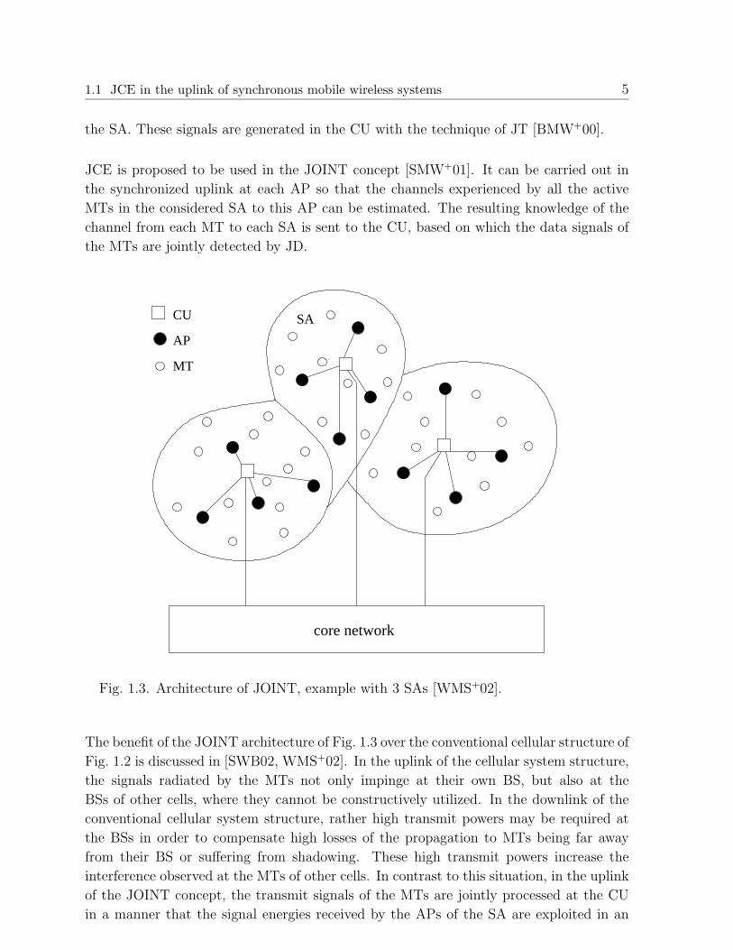
the SA. These signals are generated in the CU with the technique of JT [BMW+00].
JCE is proposed to be used in the JOINT concept [SMW+01]. It can be carried out in
the synchronized uplink at each AP so that the channels experienced by all the active
MTs in the considered SA to this AP can be estimated. The resulting knowledge of the
channel from each MT to each SA is sent to the CU, based on which the data signals of
the MTs are jointly detected by JD.
AP
core network
MT
SACU
Fig. 1.3. Architecture of JOINT, example with 3 SAs [WMS+02].
The benefit of the JOINT architecture of Fig. 1.3 over the conventional cellular structure of
Fig. 1.2 is discussed in [SWB02, WMS+02]. In the uplink of the cellular system structure,
the signals radiated by the MTs not only impinge at their own BS, but also at the
BSs of other cells, where they cannot be constructively utilized. In the downlink of the
conventional cellular system structure, rather high transmit powers may be required at
the BSs in order to compensate high losses of the propagation to MTs being far away
from their BS or suffering from shadowing. These high transmit powers increase the
interference observed at the MTs of other cells. In contrast to this situation, in the uplink
of the JOINT concept, the transmit signals of the MTs are jointly processed at the CU
in a manner that the signal energies received by the APs of the SA are exploited in an

6 Chapter 1: Introduction
optimum way characterized by simultaneously combating the impacts of inter symbol
interference (ISI) and intra-SA MAI. In the downlink of the JOINT concept, the signals
radiated by all APs are generated in the CU based on the data for each MT of the SA
in such a way that the transmit signals for each MT have minimum powers and cause
minimum interference at other MTs, and that the complexity of the MTs can be kept
low.
Whereas the target scenarios of the conventional cellular systems are mainly outdoor
environments, it is mentioned in [WMS+02] that the indoor mobile radio scenarios are
viewed as the typical application area of JOINT.
1.1.3 Time and frequency domain JCE
The radio channels in the situation shown in Fig. 1.1 can be characterized in the time
domain as channel impulse responses (CIRs). They can be equivalently characterized in
the frequency domain as channel transfer functions (CTFs). In general, the estimation
of the channel properties can be correspondingly classified into time domain channel
estimation and frequency domain channel estimation [KWC04]. In time domain channel
estimation, the training sequence is formed symbol by symbol in a certain time period,
and the estimation of the time domain channel property, i.e. CIR, is based on the receive
signal sampled in the time domain. In frequency domain channel estimation, the training
sequence is formed symbol by symbol in a certain frequency band, and the estimation of
the frequency domain channel property, i.e. CTF, is based on the receive signal sampled
in the frequency domain.
In the TD-CDMA system, the CIRs of the synchronously active users are estimated by
time domain JCE (TD-JCE), and the time domain JD is carried out afterwards. The re-
alization of JCE in the JOINT concept is a mixture of time and frequency domain channel
estimation. In the JOINT system concept, the orthogonal frequency division multiplexing
(OFDM) [NP00] based multi-carrier transmission is adopted. Although the CTFs of the
MTs are required by the frequency domain JD at the receiver and although the train-
ing sequences are allocated in the frequency domain, the CIRs are firstly estimated, and
then, based on the CIRs, the CTFs are derived by discrete Fourier transformation (DFT).
As shown in [SMW+01, MWS+02], in this way, the number of unknowns in the system
equations can be reduced to a number which does not exceed the number of equations.
In the single user OFDM scenario, it is possible to apply a complete frequency domain
channel estimation, by which the CTF of the single input single output (SISO) channel
is directly estimated without resorting to the CIR at first [CD02]. In the following, for
easier discrimination, the estimation aiming at the CTFs of channels, whether they are
directly obtained or not, is termed frequency domain channel estimation.
1.1 JCE in the uplink of synchronous mobile wireless systems 7
1.1.4 State of the art in JCE techniques
The investigation on JCE accompanies the development of wireless communication sys-
tems. In the first generation (1G) and 2G systems, JCE is not used because the re-
quirement on the system capacity in their eras was not as high as today. The capacity
demand could be met by the multiple access technique of TDMA and/or FDMA within
the allocated spectrum resource. With these techniques, the users are separated in time
or in frequency so that only single user channel estimation technique is required.
JCE is originally a multi-user based technique. It is proposed for the TD-CDMA system
and TD-SCDMA system for the 3G wireless communication systems to jointly estimate
the wireless fading channels of the multiple users that are simultaneously active in the
same frequency band and that are communicating with the same BS. In both systems,
the CIRs of the active users are jointly estimated.
As stated in Subsection 1.1.1, the wireless communication systems are stepping into the
beyond 3G or 4G which requires higher spectral efficiency for higher data rate transmission
over broadband channels. Multi-carrier transmission techniques such as OFDM [NP00] are
proposed to meet the ends and to reduce the complexity of channel equalization. Some
novel channel estimation techniques are correspondingly emerging for the multi-carrier
applications. The state of art of JCE in multi-user OFDM systems is that the training
sequence for each users is allocated symbol by symbol in frequency and the received sig-
nal is sampled in the frequency domain with the inverse discrete Fourier transformation
(IDFT) at the transmitter and the DFT at the receiver for fast implementation. As a
result, a frequency domain JCE (FD-JCE) is generally proposed to estimate the broad-
band channels of multiple users. When the problem of unknowns surpassing the number
of knowns in the equations of JCE is solved by changing the transformation domain from
frequency into time for the channel properties [SMW+01], the traditional channel estima-
tion methods, such as ML, least square (LS), weighted LS (WLS) and minimum mean
square error (MMSE) estimations [Kay93] can be applied in multi-user OFDM systems.
The JCE applied in the JOINT concept adopts this solution [WMS+02].
OFDM based systems take advantage of being robust to frequency selective fading and of
doing with one tap per sub-channel equalizers with low complexity. However, they have
also disadvantages such as the difficulty in subcarrier synchronization and sensitivity
to the frequency offsets and nonlinear amplification [NP00]. Recently, another multi-
carrier technique, filtered multi-tone (FMT), is drawing the attention of the researchers
for the design of broadband beyond 3G wireless communication systems by referring the
idea from very high speed digital subscriber lines [CEO+00, BTT02a]. Although FMT
transmission requires more complicated equalization techniques at the receiver [BTT02],
it is more robust to frequency offsets [CFW03]. Current research works on FMT based
multi-carrier transmission include the modulation, the equalization techniques and the

8 Chapter 1: Introduction
design of prototype filters [CEO02, BTT02] in single user scenarios. Future development
of FMT technique calls for its applications in multi-user and multi-antenna scenarios.
Correspondingly, a lot of investigation in these scenarios should be carried out, such as
the JCE technique.
As mentioned in Subsection 1.1.3, the JCE can be basically performed either in the time
or the frequency domain. There is up to now little theoretical analysis on the relationship
of the JCEs in these two domains. Also there are few researchers who have worked on
the relationship of the training sequences for the TD-JCE and FD-JCE.
1.2 Multi-branch systems
JCE is typically proposed to address the issue of channel estimation in synchronous multi-
user systems. In recent years, the multi-antenna transmit diversity based space-time
coding techniques [TSC98, Ala98, Fos96] emerged thanks to their potential of high channel
capacity [FG98, Tel95]. Among these techniques, the space-time block coding [Ala98] has
been proposed for the 3G WCDMA system [WCDMA]. The space-time coding techniques
are also promising for the beyond 3G systems. The channel estimation is one of the hot
topics in the investigation of multi-antenna systems [LSA99, KCW+03], which involves
the estimation of the multi-antenna fading channels at the receiver simultaneously.
Up to now, the channel estimation in multi-antenna systems and the JCE in multi-user
systems are investigated separately. However, from the signal processing point of view,
multi-antenna wireless channels and multi-user wireless channels have no intrinsical dif-
ference in the sense that both involve multiple transmit antennas that are communicating
with a receiver within the same time-frequency resources, i.e. both are involved in the
estimation of the MISO channel of Fig.1.1. So the channel estimation could be gen-
erally investigated for these two scenarios. The equivalence of channel estimation in a
multi-user scenario and a multi-antenna scenario can be observed by comparing, e.g. the
paper [SJ94] with [KCW+03, FAT03], for time domain channel estimation and the pa-
per [SMW+01] with [LSA99] for frequency domain channel estimation. This equivalence
is also mentioned in [VT01].
In the following, it is not distinguished between multiple antennas and multiple users for
channel estimation. Instead, a new term of system structure, namely multiple branches or
multi-branch scenarios, is introduced. Multi-branch systems refer to either multi-user or
multi-antenna or the combination of multi-user and multi-antenna systems. More specifi-
cally, multiple branches refer to multiple transmit branches. We do not specify the number
of receive branches or receivers. That is because, even if there are multiple receivers, each
receiver can perform signal processing independently for channel estimation. Without
1.2 Multi-branch systems 9
restricting generality, I consider only one receive branch in the thesis. That is the reason
in Fig. 1.1 only one receiver is drawn.
It is assumed that the received signals transmitted by all the branches are synchronized
at the receiver in the following.
Bandpass signal transmission in multi-branch systems can be efficiently described by the
use of the equivalent low-pass domain representation of signals, in which the signals are
expressed by their complex envelopes and vector representation of signals can be developed
[Pro95]. Moreover, the model for the channel estimation in multi-branch systems can be
decomposed into [Ver98, Kal95]:
• A physical transmission model. This represents in its interior the physical signal
transmission and establishes, with respect to its input and output, the relation
between the data symbols fed into the transmitter and the raw data estimates
available in the receiver. Consequently, this model has to work time continuously in
its interior and time discretely with respect to its input and output. In the concerned
multi-branch systems, the physical transmission takes place over a time-continuous
MISO channel of Fig. 1.1.
• A pre-processor at the transmitter before the physical transmission model and a
post-processor in the Rx after the physical transmission model.
In this thesis, the equivalent low-pass representation of the signals for the investigation of
JCE will be worked out. In Fig. 1.4, a general multi-branch system model for time domain
channel estimation over the MISO channel of Fig.1.1 is illustrated. If we assume that there
are K simultaneously active MTs in one cell or SA, with each MT k, k = 1 · · ·K, equipped
with KM,k antennas, then the total number of branches is
U =K∑
k=1
KM,k, (1.1)
with u, u = 1 · · · U , representing the index of each branch. The physical transmis-
sion model for the aforementioned multi-branch transmission in the OFDM based and
FMT based multi-carrier systems will be composed of the synthesis filter bank, the time-
continuous U × 1 MISO channel as well as the analysis filter bank, which will be further
described in Chapter 6.
As shown in Fig. 1.4, the U time domain training sequences (TD training sequences),
i.e. TD training sequence 1, TD training sequence 2, · · · , TD training sequence U , are
transmitted on the U branches. At each branch, a guard interval, which could be formed

10 Chapter 1: Introduction
by the cyclic prefix (CP) of the training sequence or any other formation, is appended to
the training sequence to avoid the interference from the consecutively transmitted data
symbols [DGE01]. The resulting U sequences for the U branches are then fed into the
physical transmission model. At the receiver the guard is discarded prior to the further
signal processing to retain the useful time domain receive signal (TD receive signal). The
radio channels experienced by all branches are estimated jointly at the receiver, i.e. a
TD-JCE is applied.
TD-JCEGuardDiscarding
Guard
Guard
Guard
sequence 2
sequence 1
TD training
TD training
TD training
sequence U
physical
tranmission
model
pre-processing
post-processing
TD receive signal
Fig. 1.4. Multi-branch system model in the time domain over the MISO channel.
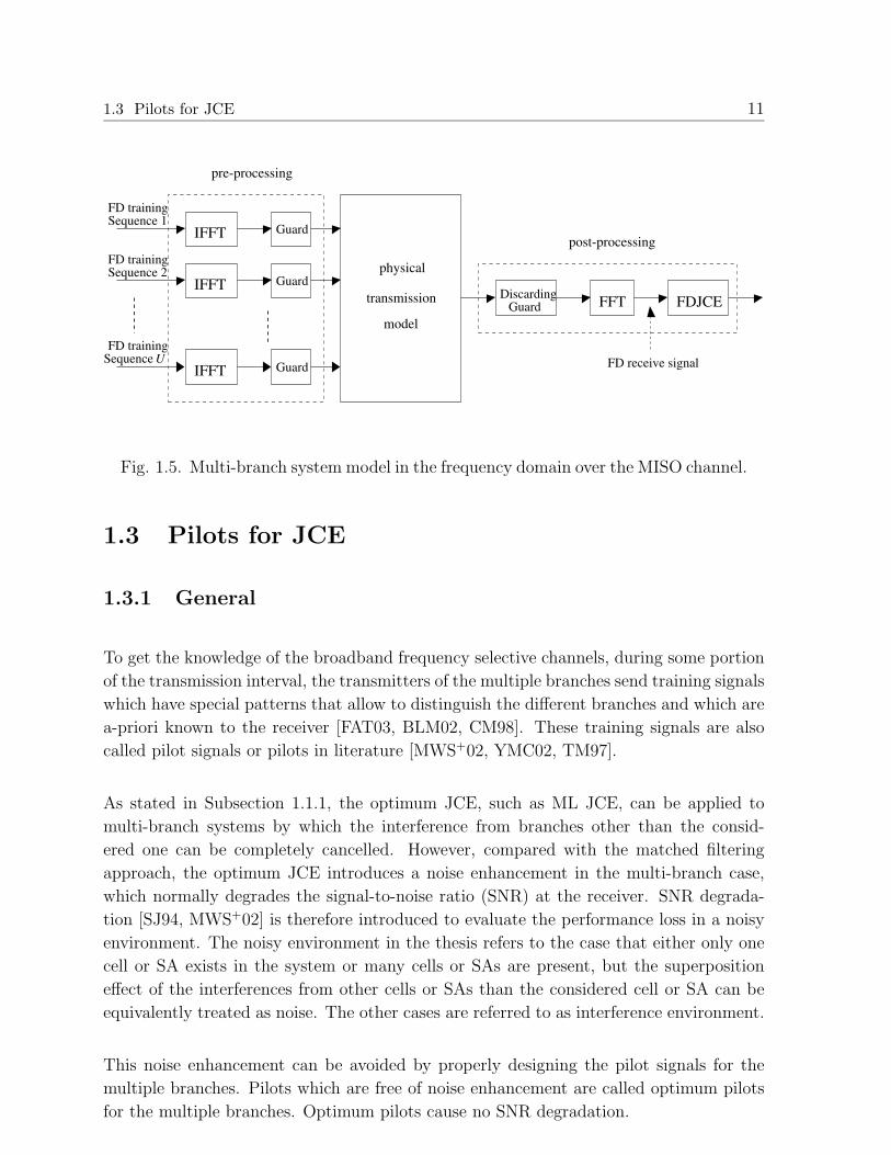
The multi-branch system model can also be described in the frequency domain as shown
in Fig. 1.5. In this structure, the U frequency domain training sequences (FD training
sequences), i.e. FD training sequence 1, FD training sequence 2, · · · , FD training se-
quence U , are transmitted on the U branches. At each branch, the training sequence is
first modulated by inverse fast Fourier transformation (IFFT) to transform signals from
frequency domain into time domain, and then appended by a guard. In OFDM systems,
which are conventionally based on the model of Fig. 1.5, the guard is achieved from the
CP of the transmit signal, i.e. at the channel estimation stage, the CP of the training
signal. The resulting signals including the guard interval are then fed into the physical
transmission model in which a MISO channel of Fig. 1.1 is experienced. At the receiver,
the guard interval is removed, and then the fast Fourier transformation (FFT) is passed.
The frequency domain receive signal (FD domain receive signal) is therefore obtained for
further signal processing. The radio channels experienced by all branches are estimated
jointly at the receiver, i.e. a FD-JCE is applied.
1.3 Pilots for JCE 11
pre-processing
Guard
Guard
Guard
FFTDiscarding
Guard
FD receive signal
FDJCE
FD training Sequence 1
FD training Sequence 2
FD training
IFFT
IFFT
IFFTSequence U
physical
transmission
model
post-processing
Fig. 1.5. Multi-branch system model in the frequency domain over the MISO channel.
1.3 Pilots for JCE
1.3.1 General
To get the knowledge of the broadband frequency selective channels, during some portion
of the transmission interval, the transmitters of the multiple branches send training signals
which have special patterns that allow to distinguish the different branches and which are
a-priori known to the receiver [FAT03, BLM02, CM98]. These training signals are also
called pilot signals or pilots in literature [MWS+02, YMC02, TM97].
As stated in Subsection 1.1.1, the optimum JCE, such as ML JCE, can be applied to
multi-branch systems by which the interference from branches other than the consid-
ered one can be completely cancelled. However, compared with the matched filtering
approach, the optimum JCE introduces a noise enhancement in the multi-branch case,
which normally degrades the signal-to-noise ratio (SNR) at the receiver. SNR degrada-
tion [SJ94, MWS+02] is therefore introduced to evaluate the performance loss in a noisy
environment. The noisy environment in the thesis refers to the case that either only one
cell or SA exists in the system or many cells or SAs are present, but the superposition
effect of the interferences from other cells or SAs than the considered cell or SA can be
equivalently treated as noise. The other cases are referred to as interference environment.
This noise enhancement can be avoided by properly designing the pilot signals for the
multiple branches. Pilots which are free of noise enhancement are called optimum pilots
for the multiple branches. Optimum pilots cause no SNR degradation.

12 Chapter 1: Introduction
In contrast to the SNR degradation in a noisy environment, the performance of JCE in
an interference environment can be evaluated by the variation coefficient [MWS+02]. It is
observed that the pilot patterns of multiple branches will also influence the performance
of JCE in interference environments [MWS+02].
Designing optimum pilots for the multiple branches is a hot topic in the research of JCE in
recent years [CM98, BLM02, Li00]. Corresponding to the equivalence of JCE in multi-user
and multi-antenna systems, which has been discussed in Section 1.2, the design of pilots in
multi-user systems [SJ94, MWS+02, CM98] and in multi-antenna systems [FAT03, Li00]
can be also equivalently coped with, although it has been developed actually in the context
of two different applications. In this thesis, the design of pilots will be carried out in the
more general multi-branch scenarios.
1.3.2 State of the art in pilot design for JCE
The development of JCE techniques is accompanied by the development of the pilot de-
sign. Since JCE has been addressed in the time and frequency domains, in multi-user and
multi-antenna systems, and is involved in single carrier and multi-carrier transmissions,
the design of pilots focuses also on such a variety of scenarios.
Up to now, the design of pilots has been addressed in the multi-user and multi-antenna
scenarios separately. In [Li00], the design criteria of optimum pilots for the multiple
transmit antennas in OFDM systems over multi-path fading channels is derived. The
properties of optimum pilots are described. But the author did not give any example of
the optimum pilots that would satisfy those properties. In [BLM02], the pilot tones, which
multiplexes the available frequency resources with the data tone, is proposed as training
sequences in OFDM systems. The property of optimum pilot tones for the multiple
transmit antennas is given [BLM02]. However, the pilot tone is just a special case of
pilot by which it is not obligatory to set some tones to be zeros. In addition, to derive
the properties of optimum pilots, some researchers also take the method of exhaustive
search [ChM00] or heuristic search [SJ94] for pilot design in multi-user systems. It is a
big challenge to the computing process when the pilot is long and when the non-binary
pilots is pursued with these search methods.
The state of the art of pilot design in the 3G wireless communication systems is that,
although the design criterium of optimum pilots with 0 dB SNR degradation has been
proposed [SJ94], there are no optimum pilots designed up to now and only suboptimum
pilots derived by heuristic search [SJ94], or pseudo noise (PN) sequences [BC02] are
proposed and applied [WCDMA, KCW+03].
Recently, with the development of beyond 3G systems, several kinds of pilots have been
presented for the JCE in multi-user OFDM systems [MWS+02], namely disjoint pilots,
1.4 Goals of this thesis 13
Walsh code based pilots and random pilots. However, up to now, there is no theoretical
derivation on the design criteria of pilots in the systems, although simulation results show
that some pilots, such as Walsh code based pilots and disjoint pilots, have 0 dB SNR
degradation. Some pilots, such as Walsh code based pilots, challenge the implementation
of OFDM transmission in the sense of peak-to-average power ratio (PAPR), which is not
yet addressed in the investigation of pilots for JCE in OFDM systems. The design of
pilots for the FMT based systems is also open.
1.4 Goals of this thesis
The previous research work concerning JCE and the design of pilots in multi-user or
multi-antenna systems will be further improved and generalized in the thesis.
The design of optimum pilots for the 3G TD-CDMA and TD-SCDMA systems, in which
time domain pilots are allocated for the multi-branch transmissions, as well as the design of
optimum pilots for the beyond 3G multi-user OFDM systems such as the JOINT concept,
in which frequency domain pilots are allocated for the multi-branch transmissions, will
be investigated through theoretical analysis. The fruits after the investigation will be the
optimum pilots for the above mentioned systems. The problem of non-linear amplifiers
will be also taken into account in the process of pilot design. Since the channel estimation
issue has never been addressed in FMT based multi-branch systems, the first focus for
these systems will be to develop the suitable JCE scheme, and then propose the suitable
pilots.
With the integration of multiple antennas and multiple users into a more general system
structure of multiple branches, the JCE as well as the pilot design issues can be more
generally dealt with. The theoretical analysis and the conclusions and results can be
applied to many systems with the generalization.
Furthermore, the time and frequency domain signal processing will be incorporated into
the research on JCE algorithm as well as the design of pilots. The relationship of the
TD-JCE and FD-JCE as well as the time and frequency domain optimum pilots will be
explained and clarified so that a special view on these issues is provided.
The goals of this thesis are:
• Propose and describe the multi-branch system model in the time and frequency
domains.
• Elaborate the JCE algorithms in both the time and the frequency domain multi-
branch systems.

14 Chapter 1: Introduction
• Derive theoretically the design criteria and properties of optimum pilots for TD-JCE
and FD-JCE in noisy environments.
• Analyze the relationship between TD-JCE and FD-JCE and clarify the relationship
of optimum pilots between TD-JCE and FD-JCE.
• Discuss and design optimum and suboptimum pilots for JCE in noisy environments
and propose some new pilots.
• Discuss the design of pilots in interference environments.
• Analyze the suitability of TD-JCE and FD-JCE to various multi-branch multi-
carrier systems.
• Investigate the performance of JCE in an OFDM based multi-branch multi-carrier
system by simulation.
• Investigate the performance of JCE in a FMT based multi-branch multi-carrier
system by simulation.
1.5 Contents and important results
This section briefly describes how the goals of this thesis presented in Section 1.4 are
achieved. The structure and organizations of this thesis is already given by the table of
contents.
Chapter 2 describes the mobile radio channel model, in particular the well known wide-
sense stationary uncorrelated scattering (WSSUS) broadband radio channel model con-
sidered in the computer simulations in Chapter 7. The statistic channel description is
adopted, by which the functions and the parameters characterizing the radio channel, such
as the time-frequency correlation function, the coherence time, the coherence bandwidth,
etc., are described. The beyond 3G channel parameters for both indoor and outdoor
scenarios are then given, based on which the indoor and outdoor broadband channels are
simulated. In addition, the interference model considered for the performance evalua-
tion of JCE in terms of variation coefficient in Chapter 3, i.e. one strong interferer from
the neighboring SA, is described. The aforementioned interference model is also used in
Chapter 5 for investigating the issue of pilot assignment in multiple SA environments.
In Chapter 3, the problems met by JCE in multi-branch systems are firstly discussed.
Three problems are paid particular attention to, i.e. the proper JCE algorithm for a
certain transmission scheme, the pilot design in noisy environments, as well as the pilot
assignment in interference environments. The following part of Chapter 3 as well as the
following chapters, i.e. Chapter 4 to Chapter 6, aim to solve these problems. After
1.5 Contents and important results 15
that, the frequency and the time domain representations of JCE are discussed separately.
For each representation, the discrete system model, the JCE algorithms, as well as the
performance evaluation of JCE, such as the SNR degradation, the mean square estimation
error (MSE) and the variation coefficient, are presented. The frequency and the time
domain representations of JCE, the frequency and the time domain JCE algorithms, as
well as the frequency and the time domain performance evaluation criteria of JCE are
proved to be equivalent in this chapter.
According to the SNR degradation evaluation of JCE in Chapter 3, the design criteria
of optimum pilots in noisy environments for both the frequency and the time domain
transmissions are derived in Chapter 4. It will be proved that the time and the frequency
domain design criteria of optimum pilots are equivalent. Based on the equivalence, the
optimum pilots designed in the frequency domain, after IDFT, will be shown to be the
optimum pilots in the time domain for JCE in multi-branch systems. On the other hand,
the optimum pilots designed in the time domain, after DFT, will be shown to be the
optimum pilots in the frequency domain for JCE in multi-branch systems. The various
optimum and suboptimum pilots for JCE in noisy environments are then constructed
according to the design criteria. As optimum pilots, the disjoint pilots, the Walsh code
based pilots and the constant amplitude zero autocorrelation (CAZAC) code based pilots
are constructed. As suboptimum pilots, the random pilots are considered for performance
comparison with the various optimum pilots in Chapter 4, 5 and 7. The numerical re-
sults of SNR degradations for the aforementioned pilots are then illustrated to verify the
theoretical analysis.
In Chapter 5, the interference environments, i.e. the multiple SA scenarios, are considered
for the pilot assignment. With the interference model of one strong interferer from the
neighboring SA as described in Chapter 2, the pilot should be assigned in multiple SA
environments in such a way that the variation coefficient for the considered SA is reduced.
The correlation property of the pilots applied to the considered SA as well as the correla-
tion property of the pilots applied to the considered SA and the neighboring SA influence
the variation coefficient. It will be shown by simulations that the arrangement of different
kinds of optimum pilots, e.g. disjoint pilots, Walsh code based pilots, and CAZAC code
based pilots, to different SAs, or the arrangement of CAZAC code based pilots to the
multiple SAs with a different mother CAZAC code in each SA, results in a good variation
coefficient performance. The latter arrangement has the additional advantage of PAPR,
which will be discussed in Chapter 6.
Chapter 6 addresses the application issues of JCE in multi-carrier systems based on OFDM
or FMT transmissions. The OFDM and FMT transmission schemes are briefly introduced
based on the description of a more general family of filter bank multi-carrier (FB-MC)
modulation. The complexity evaluation of both time domain JCE and frequency domain
JCE is then given, ending up with a curve illustrating the choice of time domain JCE
16 Chapter 1: Introduction
or frequency domain JCE according to their processing complexity. With the typical
parameters chosen for the OFDM and FMT systems, it will be shown that in broadband
channels the frequency domain JCE has less complexity for the OFDM systems, and the
time domain JCE has less complexity for the FMT systems. Another important issue for
the application of JCE is PAPR. The smaller the PAPR, the less the challenge of JCE to
the implementation of the A/D, D/A converters as well as the RF power amplifier. It will
be demonstrated that among disjoint pilots, Walsh code based pilots and CAZAC code
based pilots, CAZAC code based pilots have the minimum PAPR of 0 dB.
Chapter 7 includes the simulation results of JCE in OFDM and FMT based multi-branch
systems. The simulation results verify the theoretical analysis from Chapters 3 to 6.
A summary of this thesis in English and German is presented in Chapter 8.

17
2 Mobile radio channel model
2.1 Introduction
The mobile radio channel places fundamental limitations on the performance of wireless
communication systems. The transmission path between the transmitter and the receiver
can vary from simple line-of-sight (LOS) to one that is severely obstructed by buildings,
mountains, and foliage. The speed of motion impacts how rapidly the signal level fades
as a mobile terminal moves in space.
The received signal amplitude in mobile communications experiences fluctuations that
can be divided into large-scale fading and small-scale fading. The large-scale fading is
caused by shadowing effects in the propagation environment due to the morphology of the
environment, and the small-scale fading, or simply fading, is mainly caused by changing
interference of signals from scatterers around the receiver while the receiver moves a few
wavelengths [Par92]. Since the small-scale fading describes the rapid fluctuation of the
amplitude of a radio signal over very short travel distance of e.g. a few wavelengths
or short time durations of the order of seconds, the large-scale path loss effects can be
mitigated by power control and, hence, are generally ignored for the link level simulation,
if perfect power control is assumed.
Through the numerous measurement campaigns performed in indoor [Zol93, Kat97] and
outdoor environments [KMT96, FRB97], it is well known that in mobile radio commu-
nications a part of the electromagnetic energy radiated by the transmitter reaches the
receiver by propagating through different paths [Par92, Pap00]. The performance of dig-
ital radio communication systems is strongly affected by multi-path propagation in the
form of scattering, reflection, and refraction. The multipath in the radio channel creates
small-scale fading effects. The three most important effects of the small-scale multi-path
propagation are [Rap96]
• rapid changes in signal strength over a small travel distance or time interval,
• random frequency modulation due to varying Doppler shifts on different multi-path
signals, and
• time dispersion caused by multi-path excess delays.
The time dispersive nature of the multi-path channels is normally quantified by their
delay spread στ , which can be determined from their power delay profile [Rap96]. The
maximum multi-path excess delay τmax of the power delay profile is defined to be the time
delay during which multi-path energy is smaller than a predefined threshold. The time
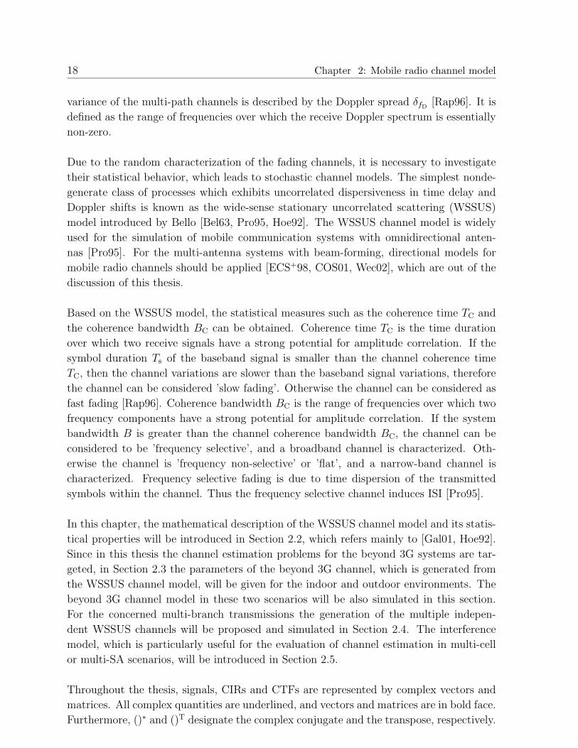
18 Chapter 2: Mobile radio channel model
variance of the multi-path channels is described by the Doppler spread δfD[Rap96]. It is
defined as the range of frequencies over which the receive Doppler spectrum is essentially
non-zero.
Due to the random characterization of the fading channels, it is necessary to investigate
their statistical behavior, which leads to stochastic channel models. The simplest nonde-
generate class of processes which exhibits uncorrelated dispersiveness in time delay and
Doppler shifts is known as the wide-sense stationary uncorrelated scattering (WSSUS)
model introduced by Bello [Bel63, Pro95, Hoe92]. The WSSUS channel model is widely
used for the simulation of mobile communication systems with omnidirectional anten-
nas [Pro95]. For the multi-antenna systems with beam-forming, directional models for
mobile radio channels should be applied [ECS+98, COS01, Wec02], which are out of the
discussion of this thesis.
Based on the WSSUS model, the statistical measures such as the coherence time TC and
the coherence bandwidth BC can be obtained. Coherence time TC is the time duration
over which two receive signals have a strong potential for amplitude correlation. If the
symbol duration Ts of the baseband signal is smaller than the channel coherence time
TC, then the channel variations are slower than the baseband signal variations, therefore
the channel can be considered ’slow fading’. Otherwise the channel can be considered as
fast fading [Rap96]. Coherence bandwidth BC is the range of frequencies over which two
frequency components have a strong potential for amplitude correlation. If the system
bandwidth B is greater than the channel coherence bandwidth BC, the channel can be
considered to be ’frequency selective’, and a broadband channel is characterized. Oth-
erwise the channel is ’frequency non-selective’ or ’flat’, and a narrow-band channel is
characterized. Frequency selective fading is due to time dispersion of the transmitted
symbols within the channel. Thus the frequency selective channel induces ISI [Pro95].
In this chapter, the mathematical description of the WSSUS channel model and its statis-
tical properties will be introduced in Section 2.2, which refers mainly to [Gal01, Hoe92].
Since in this thesis the channel estimation problems for the beyond 3G systems are tar-
geted, in Section 2.3 the parameters of the beyond 3G channel, which is generated from
the WSSUS channel model, will be given for the indoor and outdoor environments. The
beyond 3G channel model in these two scenarios will be also simulated in this section.
For the concerned multi-branch transmissions the generation of the multiple indepen-
dent WSSUS channels will be proposed and simulated in Section 2.4. The interference
model, which is particularly useful for the evaluation of channel estimation in multi-cell
or multi-SA scenarios, will be introduced in Section 2.5.
Throughout the thesis, signals, CIRs and CTFs are represented by complex vectors and
matrices. All complex quantities are underlined, and vectors and matrices are in bold face.
Furthermore, ()∗ and ()T designate the complex conjugate and the transpose, respectively.

2.2 WSSUS broadband channel model 19
The complex conjugate transpose ()∗T is also called complex Hermitian and expressed as
()H. The operator [·]x,y yields the element in the x-th row and the y-th column, and
[·]x1,y1x2,y2
yields the submatrix bounded by the rows x1, x2 and the columns y1, y2 of a
matrix in bracket. The frequency domain quantities are marked by a tilde, whereas the
time domain quantities are printed without distinguishing marks. The expressions diag(·),E· and tr· denote the diagonal matrix containing the diagonal elements of the matrix in
the argument, the expectation operation and trace operation, respectively.
2.2 WSSUS broadband channel model
2.2.1 Broadband channel characterization
The notion of WSSUS was proposed by Bello [Bel63] to model the fading phenomenon.
The WSSUS channel model is fully determined by a two-dimensional scattering function
in terms of the echo delay τ due to multi-path, and the Doppler shift fD due to the
vehicle movement [Hoe92]. It is shown [Bel63] that such a channel is effectively wide-
sense stationary (WSS) in both the time and frequency domains.
As introduced in Section 2.1, mobile radio communications suffer from multi-path prop-
agation of the transmitted signal. The transmitted signal reaches the receiver either only
as scattered signal (No line-of-sight (NLOS)) or as directed path as well as scattered signal
LOS. Let us assume the number of paths of the radio channel to be Wτ . The received
signals over the different paths experience time delays τwτ, wτ = 1 · · · Wτ , according to
the distance of the reflection points and phase rotations ϕwτ, wτ = 1 · · · Wτ . As long as
the communication environment remains unchanged and neither the transmitter nor the
receiver is moving the channel is static over time, or ’time-invariant’. With a Kronecker
delta function δ(.), the time-invariant CIR
h(τ) =1√W τ
Wτ∑
wτ=1
ejϕwτ δ(τ − τwτ) (2.1)
is obtained as the superposition of a large number Wτ of received paths [Sch89].
The Fourier transform of the time-invariant CIR h(τ) of (2.1) determines the time-
invariant CTF
h(f) =1√W τ
Wτ∑
wτ=1
ejϕwτ e−j2πfτwτ . (2.2)
A movement of either the transmitter or the receiver introduces individual Doppler shifts
fD,wτ, wτ = 1 · · · Wτ , to all Wτ propagation paths. The Doppler shifts fD,wτ
of the

20 Chapter 2: Mobile radio channel model
propagation paths introduces a ’time-variance’ to the time-invariant CIR h(τ) of (2.1)
which is caused by the phase rotation on each path over time. The Doppler shift fD,wτ
of each path is determined by the carrier frequency fc as well as the vehicle speed v and
the direction ψwτof the movement of the terminal relative to the direction from which
the signal of that path is received [Rap96]
fD,wτ=fcv
ccos(ψwτ
) = fDmaxcos(ψwτ), wτ = 1 · · · Wτ (2.3)
in which fDmax represents the maximum Doppler shift and c represents the speed of light.
With the influence of the Doppler shifts fD,wτ, wτ = 1 · · · Wτ , the time-variant CIR
h(τ, t) =1√W τ
Wτ∑
wτ=1
ejϕwτ ej2πfD,wτ tδ(τ − τwτ) (2.4)
can be obtained. By taking the Fourier transformation of the time-variant CIR h(τ, t) of
(2.4) with respect to the delay τ , the time-variant CTF
h(f, t) =1√W τ
Wτ∑
wτ=1
ejϕwτ ej2πfD,wτ te−j2πfτwτ (2.5)
can be obtained.
The time-variant CTF h(f, t) of (2.5) is a random variable and, therefore, can be statis-
tically described. According to the central limit theorem [Pro95] in the NLOS scenario,
a large number of randomly superimposed signal paths leads to a Gaussian distribution
of the time-variant CTF h(f, t) of (2.5), whose probability density function (pdf) is given
by [Pro95]
p(h) =1
2πσ2h
e−
|h|2
2σ2h , (2.6)
in which σ2h represents the variance of the time-variant CTF h(f, t) of (2.5).
The absolute value of the time-variant CTF h(f, t) of (2.5) follows a Rayleigh distribution,
whose pdf is given by [Pro95]
p(|h|) =|h|σ2
h
e−
|h|2
2σ2h . (2.7)
2.2.2 Stochastic channel description
The time delay τwτ, the phase rotation ϕwτ
and the Doppler shift fD,wτin (2.4) charac-
terize one specific channel realization related to a certain topography of the surrounding
environment. For computer simulations, a stochastic channel model which adopts the

2.2 WSSUS broadband channel model 21
statistic properties of a transmission scenario but neglects the exact topography of the
environment should be defined [Bel63, Gal01]. During the simulation process a pseudo-
random realization of the channel is generated which follows the statistical properties of
the selected transmission scenario. The actual channel can be interpreted as one possible
realization of the stochastic channel model which contains the same statistical information
as all other channel realizations [Gal01].
A number of correlation functions can be defined which are sufficient to characterize the
stochastic channel [Bel63]. The autocorrelation function of the time-variant CIR h(τ, t)
of (2.4) is given by
φh(τ1, τ2, t1, t2) = E{h(τ1, t1)h∗(τ2, t2)}. (2.8)
(2.8) describes on one hand the distribution of the average receive power over varying
delays for a given observation time, and on the other hand the changes in the distribution
of the receive power over time.
Under the assumption of a WSS stochastic process the autocorrelation function φh(τ1, τ2, t1, t2)
of (2.8) of the time-variant CIR h(τ, t) of (2.4) does not depend on the absolute time t
but depend on the time difference
4t = t2 − t1 (2.9)
of the observation times. Therefore, (2.8) turns out to be
φh(τ1, τ2,∆t) = E{h(τ1, t)h∗(τ2, t+ ∆t)}. (2.10)
Moreover, in most radio transmission situations the signal attenuations and phase rota-
tions of different propagation paths are uncorrelated. This fact is most often denoted
as uncorrelated scattering of the signals since the received signal paths are assumed to
be caused by independent scattering objects. With this assumption the autocorrelation
function φh(τ1, τ2, t1, t2) of (2.8) can be further simplified to [Hoe92]
φh(τ1, τ2,∆t) = φ
h(τ,∆t)δ(τ2 − τ1), (2.11)
which can be completely described by the autocorrelation function φh(τ,∆t).
By letting
∆t = 0 (2.12)
the autocorrelation function φh(τ,∆t) in (2.11) turns out to be
φh(τ, 0) = φ
h(τ), (2.13)
which is the average power of the time-invariant CIR h(τ) of (2.1) with respect to the
multi-path excess delay τ . φh(τ) in (2.13) is therefore also known as the power delay
profile of the channel [Pro95].

22 Chapter 2: Mobile radio channel model
Typically, the power delay profile φh(τ) in (2.13) of a radio channel is an exponentially
decreasing function with the delay τ . It is often characterized by its maximum multi-path
excess delay τmax for which the average power of the time-invariant CIR h(τ) of (2.1) is
reduced by 30 dB. The model of an exponentially decreasing power delay profile has been
adopted as part of the COST 207 [COS89] project during the development of the GSM
system. It will also be adopted in the beyond 3G WSSUS channel model in this thesis
used for the simulations in Chapter 8.
By taking the Fourier transformation of the autocorrelation function φh(τ,∆t) in (2.11)
of the time-invariant CIR h(τ) of (2.1), the scattering function
φh(τ, fD) =
∫ ∞
−∞
φh(τ,∆t)ej2π∆tfDd∆t (2.14)
is obtained, which is also recognized as the time-frequency correlation function of the
time-invariant CIR h(τ) of (2.1).
It is proved [Hoe92] that the scattering function φh(τ, fD) of (2.14) is proportional to
the joint pdf p(τ, fD) of the Doppler shifts fD and time delays τ of the independent
propagation paths, i.e.
φh(τ, fD) ∝ p(τ, fD). (2.15)
By calculating the integral of p(τ, fD) in (2.15), the marginal distributions, i.e. the pdf of
the Doppler shift fD
p(fD) ∝ φh(fD) =
∫ ∞
0
φh(τ, fD)dτ (2.16)
and the pdf of the delay τ
p(τ) ∝ φh(τ) =
∫ ∞
−∞
φh(τ, fD)dfD, (2.17)
can be obtained. The pdfs of the Doppler shift p(fD) in (2.16) and of the delay p(τ) in
(2.17) can be utilized to generate the random Doppler shifts fD,wτ, wτ = 1 · · · Wτ , and
the delays τwτ, wτ = 1 · · · Wτ , for characterizing a realization of the radio channel. It is
furthermore assumed that the two random variables of the delay τ and the Doppler shift
fD are independent and, therefore, the joint pdf p(τ, fD) in (2.15) can be written as
p(τ, fD) = p(fD)p(τ). (2.18)
The moments of the pdf of the Doppler shift p(fD) in (2.16) and the pdf of the delay p(τ) in
(2.17) can be used to characterize the properties of the stochastic channel model [Pro95].
The standard deviation of the pdf of the delay p(τ) of (2.17) is known as the delay spread
στ and the standard deviation of the pdf of the Doppler shift p(fD) of (2.16) is known as
the Doppler spread δfDof the channel, respectively.

2.2 WSSUS broadband channel model 23
Normally, the random variable of the initial phases ϕ is assumed to be uniformly dis-
tributed [Hoe92, Gal01], i.e. its pdf follows
p(ϕ) =
{12π
ϕ ∈ [0, 2π)0 else
(2.19)
The phase rotations ϕwτ, wτ = 1 · · · Wτ , in (2.4) are taken from the random samples of
ϕ.
For an exponentially decreasing power delay profile the multi-path excess delays τ are
taken from an exponential pdf [Hoe92, Gal01]
p(τ) =
{a
1−e−aτmax e−aτ 0 ≤ τ < τmax
0 else, a =
3ln(10)
τmax
(2.20)
The time delays τwτ, wτ = 1 · · · Wτ , in (2.4) are taken from the random samples of τ .
If the directions of arrival of the paths are equally probably distributed, then the pdf of
the Doppler shift fD follows a Jakes distribution [Hoe92] of
p(fD) =
1
πfDmax
√
1−
(fD
fDmax
)2|fD| < fDmax
0 else
(2.21)
fD,wτ, wτ = 1 · · · Wτ , in (2.4) are taken from the random samples of fD.
Additionally, from the autocorrelation function φh(τ,∆t) in (2.11) the time-frequency
correlation function
φh(∆f,∆t) =
∫ ∞
−∞
φh(τ,∆t)ej2π∆fτdτ. (2.22)
can be calculated, which measures the correlation of the time-variant CTF h(t, f) of (2.5)
in time and frequency directions.
Based on (2.22), the coherence time TC and the coherence bandwidth BC of the channel
can be defined, respectively, as the time and the frequency with which the absolute value
of the time correlation function φh(0,∆t) and the frequency correlation function φ
h(∆f, 0)
obtained from the time-frequency correlation function φh(∆f,∆t) of (2.22) are reduced
to half of their maximum values, i.e. [Pro95]
|φh(0, TC)| =
1
2|φ
h(0, 0)| (2.23)
and
|φh(BC, 0)| =
1
2|φ
h(0, 0)| (2.24)
are satisfied.

24 Chapter 2: Mobile radio channel model
The coherence bandwidth BC in (2.24) is inversely proportional to the delay spread στ
and is a measure for the frequency selectivity of the channel [Rap96, Pro95]. With a
broadband channel, the maximum multi-path excess delay τmax will be much larger than
the symbol duration and, therefore, will disturb consecutive symbols, i.e. the ISI appears.
For example, for a system bandwidth B of 20 MHz, the maximum multi-path excess delay
τmax of 5 µs will be approximately 100 times larger than the symbol duration Ts of 50 ns,
which is derived approximately by the inverse of the system bandwidth B. This implies
that amount of resolvable paths and severe ISI effects can be observed for the transmission
of this system over the broadband channel.
The coherence bandwidth BC can be roughly calculated as the inverse of the maximum
multi-path excess delay τmax [Rap96], i.e.
BC ≈ 1
τmax
(2.25)
satisfies.
The coherence time TC in (2.23) describes the time-variance of the channel. It is inversely
proportional to the Doppler spread σfD[Rap96]. For a coherence time TC much greater
than the symbol duration Ts the channel will not change within the duration of amount of
symbols. Therefore, the coherence time influences the frequency of carrying out channel
estimation and of inserting pilots. The shorter the coherence time, the more often the
channel estimation should be carried out.
The coherence time TC can be roughly estimated as the inverse of the maximum Doppler
shift fDmax , i.e.
TC ≈ 1
fDmax
(2.26)
satisfies.
2.3 Beyond 3G channel
2.3.1 Channel parameters
The application scenarios of the channel estimation techniques, although are not limited
to, are the beyond 3G systems in this thesis. The beyond 3G channel is constructed
as the WSSUS channel described in Section 2.2 with specific parameters. To simulate
the performance of JCE in various beyond 3G system concepts, which will be focused in
Chapter 8, it is necessary to have a common channel parameter basis in the simulations in
order to come to comparable results. Mainly two scenarios, an indoor scenario with lower
2.3 Beyond 3G channel 25
mobility and an outdoor scenario with higher mobility are defined, which are referred to
also as the indoor channel and the outdoor channel. The parameters of the considered
beyond 3G indoor and outdoor channels are summarized in Table 2.1 [Gal01].
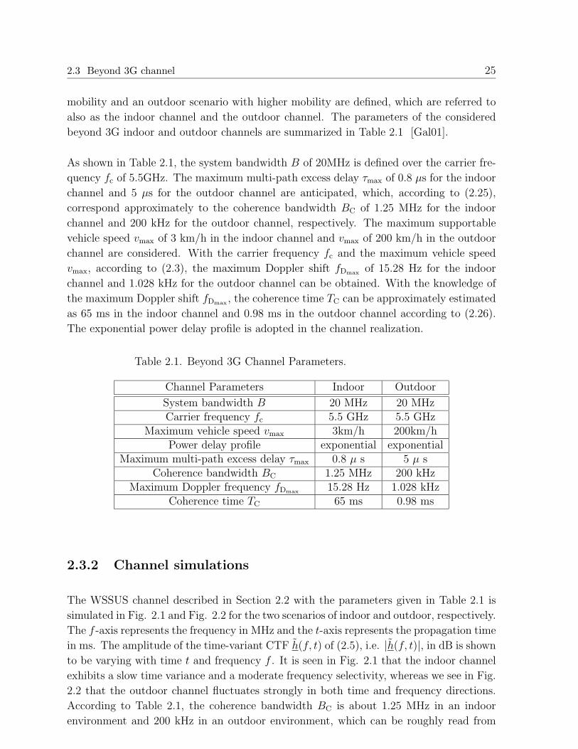
As shown in Table 2.1, the system bandwidth B of 20MHz is defined over the carrier fre-
quency fc of 5.5GHz. The maximum multi-path excess delay τmax of 0.8 µs for the indoor
channel and 5 µs for the outdoor channel are anticipated, which, according to (2.25),
correspond approximately to the coherence bandwidth BC of 1.25 MHz for the indoor
channel and 200 kHz for the outdoor channel, respectively. The maximum supportable
vehicle speed vmax of 3 km/h in the indoor channel and vmax of 200 km/h in the outdoor
channel are considered. With the carrier frequency fc and the maximum vehicle speed
vmax, according to (2.3), the maximum Doppler shift fDmax of 15.28 Hz for the indoor
channel and 1.028 kHz for the outdoor channel can be obtained. With the knowledge of
the maximum Doppler shift fDmax , the coherence time TC can be approximately estimated
as 65 ms in the indoor channel and 0.98 ms in the outdoor channel according to (2.26).
The exponential power delay profile is adopted in the channel realization.
Table 2.1. Beyond 3G Channel Parameters.
Channel Parameters Indoor Outdoor
System bandwidth B 20 MHz 20 MHzCarrier frequency fc 5.5 GHz 5.5 GHz
Maximum vehicle speed vmax 3km/h 200km/hPower delay profile exponential exponential
Maximum multi-path excess delay τmax 0.8 µ s 5 µ sCoherence bandwidth BC 1.25 MHz 200 kHz
Maximum Doppler frequency fDmax 15.28 Hz 1.028 kHzCoherence time TC 65 ms 0.98 ms
2.3.2 Channel simulations
The WSSUS channel described in Section 2.2 with the parameters given in Table 2.1 is
simulated in Fig. 2.1 and Fig. 2.2 for the two scenarios of indoor and outdoor, respectively.
The f -axis represents the frequency in MHz and the t-axis represents the propagation time
in ms. The amplitude of the time-variant CTF h(f, t) of (2.5), i.e. |h(f, t)|, in dB is shown
to be varying with time t and frequency f . It is seen in Fig. 2.1 that the indoor channel
exhibits a slow time variance and a moderate frequency selectivity, whereas we see in Fig.
2.2 that the outdoor channel fluctuates strongly in both time and frequency directions.
According to Table 2.1, the coherence bandwidth BC is about 1.25 MHz in an indoor
environment and 200 kHz in an outdoor environment, which can be roughly read from
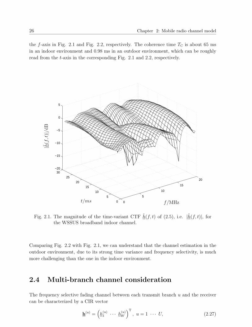
26 Chapter 2: Mobile radio channel model
the f -axis in Fig. 2.1 and Fig. 2.2, respectively. The coherence time TC is about 65 ms
in an indoor environment and 0.98 ms in an outdoor environment, which can be roughly
read from the t-axis in the corresponding Fig. 2.1 and 2.2, respectively.
0
5
10
15
20
0
5
10
15
20
25
30−20
−15
−10
−5
0
5
|h(f,t
)|/dB
t/ms f/MHz
Fig. 2.1. The magnitude of the time-variant CTF h(f, t) of (2.5), i.e. |h(f, t)|, forthe WSSUS broadband indoor channel.
Comparing Fig. 2.2 with Fig. 2.1, we can understand that the channel estimation in the
outdoor environment, due to its strong time variance and frequency selectivity, is much
more challenging than the one in the indoor environment.
2.4 Multi-branch channel consideration
The frequency selective fading channel between each transmit branch u and the receiver
can be characterized by a CIR vector
h(u) =(
h(u)1 · · · h(u)
W
)T
, u = 1 · · · U, (2.27)

2.4 Multi-branch channel consideration 27
0
5
10
15
20
0
5
10
15
20
25
30−20
−15
−10
−5
0
5
|h(f,t
)|/dB
t/msf/MHz
Fig. 2.2. The amplitude of the time-variant CTF h(f, t) of (2.5), i.e. |h(f, t)|, for theWSSUS broadband outdoor channel.
of dimension W , with W representing the number of channel coefficients. Different from
the CIR expression h(τ) in (2.1) with a number Wτ of paths, in the vector expression
(2.27) for the CIR h(u), only a limited number W of channel coefficients is considered.
With (2.27) the total CIR vector for the U branches
h =(
h(1)T · · · h(U)T)T
(2.28)
of dimension UW is obtained.
The correlation matrix of the total CIR vector h of (2.28) is expressed as [Wec02]
Rh = E{h hH}. (2.29)
If the WSSUS channel realizations for any two branches are uncorrelated, the correlation
matrix Rh of (2.29) should be diagonal matrix.
28 Chapter 2: Mobile radio channel model
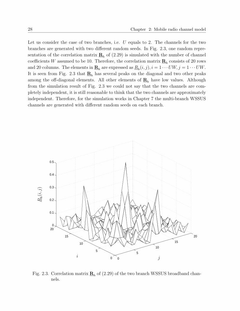
Let us consider the case of two branches, i.e. U equals to 2. The channels for the two
branches are generated with two different random seeds. In Fig. 2.3, one random repre-
sentation of the correlation matrix Rh of (2.29) is simulated with the number of channel
coefficients W assumed to be 10. Therefore, the correlation matrix Rh consists of 20 rows
and 20 columns. The elements in Rh are expressed as Rh(i, j), i = 1 · · ·UW, j = 1 · · ·UW .
It is seen from Fig. 2.3 that Rh has several peaks on the diagonal and two other peaks
among the off-diagonal elements. All other elements of Rh have low values. Although
from the simulation result of Fig. 2.3 we could not say that the two channels are com-
pletely independent, it is still reasonable to think that the two channels are approximately
independent. Therefore, for the simulation works in Chapter 7 the multi-branch WSSUS
channels are generated with different random seeds on each branch.
0
5
10
15
20
0
5
10
15
200
0.1
0.2
0.3
0.4
0.5
Rh(i,j
)
i j
Fig. 2.3. Correlation matrix Rh of (2.29) of the two branch WSSUS broadband chan-nels.
2.5 Interference model 29
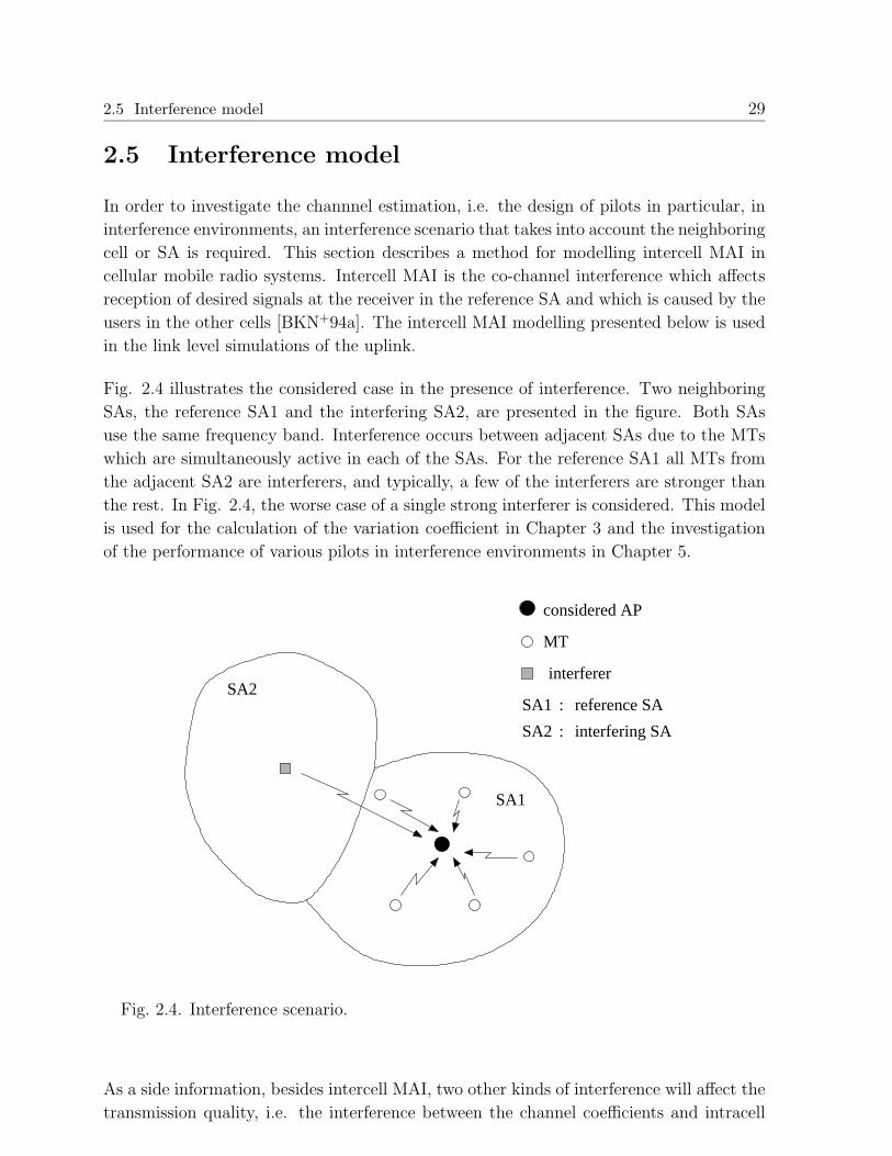
2.5 Interference model
In order to investigate the channnel estimation, i.e. the design of pilots in particular, in
interference environments, an interference scenario that takes into account the neighboring
cell or SA is required. This section describes a method for modelling intercell MAI in
cellular mobile radio systems. Intercell MAI is the co-channel interference which affects
reception of desired signals at the receiver in the reference SA and which is caused by the
users in the other cells [BKN+94a]. The intercell MAI modelling presented below is used
in the link level simulations of the uplink.
Fig. 2.4 illustrates the considered case in the presence of interference. Two neighboring
SAs, the reference SA1 and the interfering SA2, are presented in the figure. Both SAs
use the same frequency band. Interference occurs between adjacent SAs due to the MTs
which are simultaneously active in each of the SAs. For the reference SA1 all MTs from
the adjacent SA2 are interferers, and typically, a few of the interferers are stronger than
the rest. In Fig. 2.4, the worse case of a single strong interferer is considered. This model
is used for the calculation of the variation coefficient in Chapter 3 and the investigation
of the performance of various pilots in interference environments in Chapter 5.
interfering SA
SA1
SA2
MT
considered AP
interferer
SA1
SA2
:
:
reference SA
Fig. 2.4. Interference scenario.
As a side information, besides intercell MAI, two other kinds of interference will affect the
transmission quality, i.e. the interference between the channel coefficients and intracell
30 Chapter 2: Mobile radio channel model
MAI. ISI is caused by the superposition of signal components originating in temporally
adjacent transmitted data symbols, as mentioned in Section 2.1, while intracell MAI is
caused by the user signals other than the desired user signal those are simultaneously
present in the same frequency band in the cell or SA under consideration [Pro95, Kle96].
Both the interference between the channel coefficients and intracell MAI can be eliminated
by the well-designed JCE scheme [SJ94, SMW+01], which will be discussed in Chapter
3. However, the intercell MAI cannot be cancelled with the traditional single branch
channel estimation scheme and even not with the JCE scheme, since the pilots used by
the branches in the neighboring cell or SA are unknown to the receivers in the considered
cell or SA.

31
3 JCE in multi-branch systems
3.1 Introduction
As mentioned in Subsection 1.1.3, the channel estimation can be carried out either in the
time domain or in the frequency domain, corresponding to the signals and the channels
represented either in the time domain or in the frequency domain. The JCE processed
in different domains has different typical application scenarios, such as the TD-JCE in
the uplink of synchronous multi-user CDMA systems and the FD-JCE in the uplink of
synchronous multi-user OFDM systems. However, the application of JCE is not restricted
to these typical scenarios. For example, the FD-JCE can be also applied to the multi-
antenna OFDM systems [LSA99]. In this chapter, the discussion of JCE is not limited to
any particular transmission scenario, but generally treated by considering multi-branch
systems with signals represented in both the time and frequency domains. The derivations
and conclusions may be applied to many applications of wireless communication systems,
such as single carrier multi-user CDMA systems [SJ94], OFDM based multi-carrier multi-
user systems [SMW+01, MWS+02, KMW+04] as well as FMT based multi-carrier multiple
antenna systems [KWC04a].
The frequency domain representation and the time domain representation of a multi-
branch linear transmission system are inherently equivalent. For example, the equivalence
between the time and the frequency domain representations of JCE will be discussed in
Section 3.4. Based on this observation, the multi-branch system is mainly represented in
one domain, e.g. the frequency domain in this chapter. A discrete frequency model of
the multi-branch systems will be obtained in Subsection 3.3.1. Various FD-JCE schemes,
discussed in Subsection 3.3.2, will be derived based on the discrete frequency model. The
equivalence between the discrete time representation and the discrete frequency represen-
tation for the multi-branch systems can be observed by the shift property of the DFT,
which will be discussed in Subsection 3.4.2. Based on this equivalence, the discrete time
model for the multi-branch systems and the various TD-JCE schemes will be obtained
from their frequency domain counterparts in Subsections 3.4.3 and 3.4.4, respectively.
As stated in Subsection 1.3.1, the performance of JCE can be evaluated in noisy en-
vironments by the SNR degradation and in interference environments by the variation
coefficient. The SNR degradation provides us with the numerical results of the rela-
tive performance loss for a certain JCE algorithm compared with a reference method.
If the reference method is chosen as the matched filtering JCE (MF-JCE) with neglect-
ing interference between the channel coefficients and MAI [SJ94, Kle96], then the SNR
degradation describes the performance loss of a certain JCE algorithm for a multi-branch
system with respect to the single-branch scenario. The variation coefficient provides us

32 Chapter 3: JCE in multi-branch systems
with the statistical fluctuation of interference [MWS+02]. Moreover, if we aim to statis-
tically evaluate the difference of the estimated channel with respect to the real channel,
then the MSE [Kay93] can be introduced.
The performance evaluation of FD-JCE in terms of the SNR degradation, the MSE and
the variation coefficient will be derived in Subsections 3.3.3, 3.3.4 and 3.3.5, respectively.
The performance evaluation of TD-JCE in terms of the SNR degradation and the MSE
will be derived in Subsections 3.4.5 and 3.4.6, respectively.
3.2 Description of the problems of JCE
Before investigating JCE for the linear multi-branch transmission systems, the problems
met by JCE should be explained. Without loss of generality, the signals and variables in
this section will be expressed in the time domain, i.e. Fig. 1.4 will be referred to.
As shown in Fig. 1.4, the multi-branch system comprises U branches. U is the sum of the
number of all antenna elements of the K MTs together, where each MT k, k = 1 · · ·K,
is equipped with KM,k antennas, see (1.1). In order to carry out JCE, U pilots are
transmitted by the U branches so that the CIR vectors h(u), u = 1 · · ·U, of (2.27) of the
U radio channels of Fig. 1.1 can be simultaneously distinguished and estimated at the
receiver. At each branch u, a branch specific pilot vector, i.e. the TD training sequence
u, u = 1 · · ·U , in Fig. 1.4,
p(u) =(
p(u)
1· · · p(u)
Lp
)T
, u = 1 · · · U, (3.1)
of dimension Lp, which is a-priori known at the receiver, is considered in the channel
estimation process. p(u) of (3.1) is composed of Lp discrete time complex symbols p(u)lp, u =
1 · · · U, lp = 1 · · · Lp.
With a linear system model, according to Fig. 3.2, the problems of JCE can be described.
As shown in Fig. 3.2, the task of JCE in a multi-branch system is that, from a receive
signal vector
r =(
r1 · · · rLp
)T
(3.2)
of dimension Lp, based on the a-priori knowledge of the number of channel coefficients W
as well as the pilot vector p(u), u = 1 · · · U, of (3.1) transmitted by all the U branches,
the CIR vectors h(u), u = 1 · · · U , of (2.27) experienced by all the U branches are jointly
estimated as the estimated CIR vectors
h(u)
=(
h(u)
1 · · · h(u)
W
)T
, u = 1 · · · U, (3.3)

3.2 Description of the problems of JCE 33
of dimension W for the U branches, based on which a total estimated CIR vector
h =
(
h(1)T · · · h
(U)T)T
(3.4)
of dimension UW is obtained.
It is worth noting that the dimension of r of (3.2) is only then equal to Lp, if we work
with a prefix before the pilot vector p(u) of (3.1) and do not consider the total of the
receive signal. This statement can be illustrated in Fig. 3.1 for the receive signals for the
u-th, u = 1 · · ·U , branch, i.e. r(u)1 to r
(u)Lp+W−1, which are obtained from the convolution
of the transmit pilot signal p(u) of (3.1) of dimension Lp and the CIR h(u) of (2.27) of
dimension W . The relationship between r(u)lp
, lp = 1 · · ·Lp, and the elements r(lp) in the
receive signal vector r of (3.2) is
r(lp) =U∑
u=1
r(u)lp, lp = 1 · · ·Lp. (3.5)
The shadowed parts in Figs. 3.1 (c) and (d) illustrate the data symbols transmitted after
the pilot signal p(u) of (3.1). It is seen in Fig. 3.1 that with a prefix in front of the
pilot signal p(u) of (3.1), r(u)1 to r
(u)Lp
correspond to the receive signals which are free of
the interference from the consecutively transmitted data symbols, while r(u)Lp+1 to r
(u)Lp+W−1
correspond to the receive signals with the interference. For channel estimation, only the
Lp receive signals which are free of the interference, i.e. r(u)1 to r
(u)Lp
, are taken into account.
If for the received noise vector
n =(
n1 · · · nLp
)T
(3.6)
of dimension Lp the covariance matrix
Rn = E{n nH} (3.7)
is also a-priori known, this knowledge can be used to improve the estimation performance.
According to estimation theory [Kay93], based on various algorithms such as MF, LS,
WLS and MMSE, various estimators can be correspondingly developed. All these esti-
mators require the a-priori knowledge of the number W of channel coefficients as well as
the transmitted pilot vectors p(u), u = 1 · · · U, of (3.1). The WLS estimators require
additionally the a-priori knowledge of the noise covariance matrix Rn of (3.7), while the
MMSE estimator requires additionally the a-priori knowledge of the noise covariance ma-
trix Rn of (3.7) and the covariance matrix of the total CIR vector Rh of (2.29). The
MMSE estimator normally outperforms the other estimators. However, more a-priori
knowledge is needed by the MMSE estimator which makes the MMSE estimator more

34 Chapter 3: JCE in multi-branch systems
(d)
Prefix
(a)
(b)
(c)
Prefix
Prefix
Prefix
h(u)1
h(u)1
h(u)1
h(u)1
h(u)W
h(u)W
h(u)W
h(u)W
p(u)1
p(u)1
p(u)1
p(u)1
p(u)Lp
p(u)Lp
p(u)Lp
p(u)Lp
r(u)1
r(u)Lp
r(u)Lp+1
r(u)Lp+W−1
Fig. 3.1. Generation of the receive signals.
channel
a-priori
knowledge
noise covariance
matrix
Noise
JCE
pilot signals channel dimension
transmitter
p(u), u = 1 · · · U
p(u), u = 1 · · · U
W
h(u), u = 1 · · · U
Rn
n
r h(u), u = 1 · · · U
Fig. 3.2. Description of the problems of JCE.
complicated to implement than the other estimators and which restricts its applications
in practical systems. Therefore, the MMSE estimation is not considered in this thesis.
3.2 Description of the problems of JCE 35
If the noise vector n of (3.6) is complex Gaussian with power σ2 of the real and the
imaginary parts, i.e. the noise covariance matrix satisfies
Rn = 2σ2ILp , (3.8)
in which ILp is a Lp × Lp identity matrix, then the WLS estimate will become the LS
estimate and both are identical to the ML estimate [Kay93].
The unbiased estimation of the total CIR vector h of (2.28) requires
E{h} = h. (3.9)
An estimation by which (3.9) cannot be fulfilled is biased. Both the LS and the WLS esti-
mations are unbiased [Kay93]. If the noise n is not Gaussian, then the WLS estimation is
expected to outperform the LS estimation. MF estimation is biased since the interference
between the channel coefficients is not considered.
From the above discussions, the performance of channel estimation varies with the avail-
ability of the a-priori knowledge, i.e. the number of channel coefficients W , the trans-
mitted pilot vectors p(u), u = 1 · · ·U , of (3.1) as well as the noise covariance matrix Rn
of (3.7). Besides, different channel estimation algorithms such as MF, LS and WLS es-
timations have different implementation complexity. Therefore, the first problem of JCE
is to select a suitable algorithm for the multi-branch applications by jointly considering
the available a-priori knowledge, the noise covariance matrix Rn of (3.7), the estimation
performance and the complexity.
It is observed that the performance of JCE in terms of MSE or SNR degradation depends
on the transmitted pilots [SJ94, MWS+02]. For example, for the widely applied LS JCE
algorithm, if the estimated CIR vector h(u)
of (3.3) is required to statistically deviate as
little as possible from the true CIR vector h(u) of (2.27) in the sense of MSE [Kay93],
then some pilots can result in the minimum achievable MSE [KMW+04]. With these
pilots, the SNR degradation of a particular channel estimation scheme in comparison to
the SNR-minimized scheme, i.e. the MF channel estimation, is also minimized, i.e. 0 dB
SNR degradation can be achieved [SJ94, MWS+02]. The pilots by which the minimum
MSE and the 0 dB SNR degradation can be achieved are called the optimum pilots.
Therefore, the second problem met by JCE in the multi-branch systems is how to design
the optimum pilots for the multiple branch transmissions by which both the MSE and
the SNR degradation can be minimized.
The performance of JCE in noisy environments is generally evaluated by the SNR degra-
dation [SJ94, SMW+01]. In interference environments, i.e. if more than one cell or SA is
considered in the systems, it is normally the interference originating in the adjacent cells
and SAs that limits the system performance. The smaller the fluctuation of the interfer-
ence, the more similar the behavior of the interference to additive white Gaussian noise

36 Chapter 3: JCE in multi-branch systems
(AWGN), and the better the overall system performance. The performance of JCE in
interference environments is generally evaluated by the variation coefficient [Fis76]. The
smaller the variation coefficient, the better the overall system performance. It is observed
that the variation coefficient for JCE depends on the pilots being chosen for the reference
SA and the neighboring SA [MWS+02]. Therefore, the third problem met by JCE is how
to design the pilots for the branches in the reference SA and its neighboring SAs so that
the variation coefficient can be reduced and simultaneously the SNR degradation in each
SA can be minimized.
The above mentioned three problems should be solved by the investigation of JCE no
matter the TD-JCE or the FD-JCE is carried out. Besides, the implementation of a JCE
algorithm in the time domain or in the frequency domain has different complexity. For a
certain transmission scheme of a wireless communication system, it is also the task of the
system designer to choose a JCE scheme processed in a suitable domain with moderate
complexity to meet the overall system requirements.
Envisaging the problems of JCE in multi-branch systems described above, in this chapter
I focus on the first problem of deriving the JCE algorithms for multi-branch systems.
Besides, the performance criteria of JCE such as the MSE, the SNR degradation and the
variation coefficient will be also discussed in this chapter. In Chapter 4 the second problem
of designing the optimum pilots for the multi-branch systems in noisy environments with
one considered SA will be dealt with. The third problem of how to assign pilots for
the multiple branches in the considered SA and its neighboring SAs will be discussed in
Chapter 5. The choice of the suitable process domain for JCE based on the complexity
evaluation of time and frequency domain processing will be addressed in Chapter 6.
3.3 Frequency domain representation of JCE
3.3.1 Discrete frequency model
In this section, the discrete frequency transmission model based on the frequency domain
multi-branch transmission of Fig. 1.5 considering the MISO channel of Fig. 1.1 will be
described. Since the transmitted signals shown in the physical transmission model of Fig.
1.5 are normally represented in the time domain, the considered signals before the IFFT
at the transmitter and after the FFT at the receiver are represented in the frequency
domain.
The signals on each branch u, u = 1 · · ·U , are supposed to be transmitted on NF subcar-
riers. It is assumed that each branch u experiences a frequency selective channel whose
CIR vector h(u) of (2.27) can be represented by W channel coefficients. At each branch

3.3 Frequency domain representation of JCE 37
u, u = 1 · · · U , a branch specific frequency domain pilot vector, i.e. the FD training
sequence u in Fig. 1.5,
p(u) =(
p(u)
1· · · p(u)
NF
)T
, u = 1 · · · U, (3.10)
of dimension NF is transmitted. Without loss of generality, the pilot vector p(u) of (3.10)
on each branch is assumed to occupy all the NF subcarriers for channel estimation, com-
posing an OFDM symbol. The U pilot vectors p(u), u = 1 · · · U , are assumed to have
the same energy
Ep =1
2p(u)Hp(u), u = 1 · · ·U. (3.11)
The pilot and the data are assumed to be multiplexed in time, i.e. OFDM symbol by
symbol. Fig. 3.3 illustrates the multiplexing block structure of pilot and data concerned
for a frequency representation of the multi-branch systems of Fig. 1.5. Notice that trans-
missions on different branches can be introduced as different transmissions in the spatial
domain.
After the IDFT of each pilot vector p(u) of (3.10), a time domain pilot vector p(u) of (3.1)
of dimension Lp is obtained. Lp is equal to NF. With the Fourier matrix [BC02]
F =
1 1 1 . . . 1
1 e−j 2π
NF e−j 2π×2
NF... e
−j2π(NF−1)
NF
1 e−j 2π×2
NF e−j 2π×4
NF... e
−j2π×2(NF−1)
NF
......
.... . .
...
1 e−j
2π(NF−1)
NF e−j
2π×2(NF−1)
NF... e
−j2π(NF−1)2
NF
(3.12)
of dimension NF × NF, the relationship between the frequency domain pilot vector p(u)
of (3.10) and the time domain pilot vector p(u) of (3.1) is given by
p(u) = F p(u), u = 1 · · · U. (3.13)
As indicated in Fig. 1.5, a guard vector
g(u) =(
g(u)
1· · · g(u)
LG
)T
, u = 1 · · · U, (3.14)
of dimension LG is then placed in front of the time domain pilot vector p(u) of (3.1) for
transmission to provide protection between two transmit blocks. With W denoting the
number of channel coefficients, the condition LG > W − 1 should be satisfied for the
interference free transmission. The time multiplexing structure of the pilot vector p(u) of
(3.1) and the guard vector g(u) of (3.14) is illustrated in Fig. 3.4.
In [SJ94], the extended pilot vector
p(u)
E= (g(u)T p(u)T)T (3.15)

38 Chapter 3: JCE in multi-branch systems
FD tr
aini
ng s
eque
nce
,
i.e.
F
Space
Time
Dat
a
Dat
a
Dat
a
Dat
a
Frequency
U
FD tr
aini
ng s
eque
nce
1, i.
e.
N
p(1
)
p(U
)
Fig. 3.3. Multiplexing structure of the pilot and the data concerned for a frequencydomain representation of the multi-branch system of Fig. 1.5.
Time
1 2 LpLpLp − LG + 1
︸ ︷︷ ︸
g(u)
︸ ︷︷ ︸
p(u)
LG elements︷ ︸︸ ︷
Lp elements︷ ︸︸ ︷
Fig. 3.4. Time multiplexing structure of the pilot vector p(u) of dimension Lp and
the guard vector g(u) of dimension LG.
of dimension Lp plus LG is considered in the pilot design process for each branch u, u =
1 · · ·U . At the receiver the leading LG received samples are discarded and only the
Lp received samples are retained for channel estimation. For the U branches, with the

3.3 Frequency domain representation of JCE 39
assumption that the extended pilot vectors p(u)E, u = 1 · · ·U, of (3.15) for the U branches
are independently designed, the degree of freedom f for designing the U extended pilot
vectors is [SJ94]
f = U(LG + Lp), (3.16)
provided that an exhaustive search method is used for the pilot design [SJ94]. The degree
of freedom f is reduced if the extended pilot vector p(u)E
of (3.15) of each branch consists
of p(u) of dimension Lp plus LG elements taken from p(u) [SJ94]. The degree of freedom
f for designing the U extended pilot vectors in this case will be
f = ULp. (3.17)
(3.17) can be fulfilled by introducing a cyclic prefix to the pilot vector p(u) of (3.1). This
cyclic prefix on the other hand forms the guard vector g(u) of (3.14), which is composed
of the cyclic shifts of the last LG symbols of the pilot vector p(u) of (3.1), i.e.
g(u) =(
p(u)
Lp−LG+1· · · p(u)
Lp−1p(u)
Lp
)T
, u = 1 · · · U. (3.18)
As a side information, if, instead of the pilot, the data are transmitted, the cyclic prefix
structure will be beneficial to the equalization and detection. With the cyclic prefix, the
linear convolution of the transmitted signal with the CIR becomes the circular convo-
lution so that the time domain convolution will be equivalent to the frequency domain
multiplication [BT02]. With this equivalence, the frequency domain equalization can be
realized by just multiplying the inverse of the CTF matrix by the frequency domain re-
ceive signal [BP95]. Hence the complexity of equalization can be significantly reduced,
especially if broadband single carrier systems are considered [FAB02]. Comparing with
the time domain equalization to broadband single carrier systems, where a huge number
of channel coefficients must be estimated, the frequency domain equalization is much less
complicated because the equalization is performed on a block of data at a time and the
operations on this block involve an efficient FFT operation and a simple channel inver-
sion operation [FAB02]. This makes the frequency domain equalization, and originally,
the structure with a cyclic prefix, particularly attractive to the broadband applications.
In OFDM-based multi-carrier systems the cyclic prefix is applied to the transmitted signal
so that the receive signals contain mutually orthogonal sinusoidal sections with constant
envelope, which are in the receiver processed by FFT [NP00].
The radio channel between each transmit branch u and the receiver can be characterized
by the CIR vector h(u) of (2.27), or by a CTF vector
h(u)
=(
h(u)
1 · · · h(u)
NF
)T
, u = 1 · · · U, (3.19)
of dimension NF. With (3.19), the total CTF vector
h =
(
h(1)T · · · h
(U)T)T
(3.20)

40 Chapter 3: JCE in multi-branch systems
of dimension UNF of all U branches is obtained.
With the typical OFDM system applications of the frequency domain multi-branch system
model of Fig. 1.5, it is verified that the number of channel coefficients W of the CIR vector
h(u) of (2.27) is smaller than the dimension NF of the CTF vector h(u)
of (3.19) [NP00].
Let us consider a blockdiagonal matrix
FW,tot =
[
F
]1,1
NF,W. . . 0
.... . .
...
0 . . .[
F
]1,1
NF,W
(3.21)
of dimension (UNF) × (UW ), whose blocks
FW =[
F
]1,1
NF,W(3.22)
are matrices containing the first W columns of the Fourier matrix F of (3.12). With
(3.21), the total CIR vector h of (2.28) and the total CTF vector h of (3.20) are related
by [SMW+01, MWS+02]
h = FW,toth. (3.23)
With a branch specific pilot matrix
P(u)
= diag(
p(u)
1· · · p(u)
NF
)T
, u = 1 · · · U, (3.24)
of dimension NF ×NF, whose diagonal elements are composed of the components of p(u)
of (3.10), a total pilot matrix
P =(
P(1) · · · P
(U))
(3.25)
of dimension NF × (UNF) is obtained.
With a noise vector
n =(n1 · · · nNF
)T(3.26)
of dimension NF at the receiver, together with the total CTF vector h of (3.20) and the
total pilot matrix P of (3.25), the FD receive signal vector
r = P h + n (3.27)
illustrated in Fig. 1.5 and having the dimension NF is obtained.

3.3 Frequency domain representation of JCE 41
There are UNF unknown frequency samples in the total CTF vector h of (3.20) but only
NF samples in the frequency domain receive signal vector r of (3.27). Therefore, the linear
set of equations described by (3.27) is underdetermined.
Substituting (3.23) into (3.27) gives
r = P FW,tot︸ ︷︷ ︸
G
h + n, (3.28)
in which G is a matrix of dimension NF × (UW ).
In the linear multi-branch system described by (3.28), there are UW unknown channel
coefficients and NF received samples. In the case
NF ≥ UW, (3.29)
(3.28) is an overdetermined or a determined linear set of equations. (3.28) is assumed
to be fulfilled in the following and will be used to derive the FD-JCE algorithms in the
Subsection 3.3.2.
3.3.2 FD-JCE algorithms
In this subsection, three different FD-JCE algorithms will be derived based on the dis-
crete frequency representation of the multi-branch transmission model described in Sub-
section 3.3.1. In order to reduce the number of unknowns, the total CIR vector h of (2.28)
is firstly estimated, based on which the total CTF vector h of (3.20) is obtained. In both
cases, the pilot vectors contained in matrix G and the received signal vector r in (3.28)
are expressed in the frequency domain. According to the classification in Subsection 1.1.3,
the estimation in both cases is called FD-JCE.
Under the assumption of the linear system, the FD-JCE at the receiver in Fig. 1.5 is
assumed to be linear by multiplying the receive signal vector r in (3.28) with an estimation
matrix M of dimension (UW ) ×NF, i.e.
h = M r = M G h + M n. (3.30)
Various choices of the estimation matrix M result in various FD-JCE algorithms. The
unbiased estimation requires (3.9) to be fulfilled.
Without any a-priori knowledge about the statistical properties of the noise n of (3.26),
the conventional method of digital signal processing in the receiver for channel estimation
is correlation by an estimation matrix M matched to the matrix G [Kay93], i.e.
M = GH. (3.31)

42 Chapter 3: JCE in multi-branch systems
Substituting (3.31) into (3.30), a frequency domain MF JCE (FD-MF-JCE)
hMF = GHr = G
HG h + G
Hn. (3.32)
of the total CIR vector h of (2.28) is obtained. The a-priori knowledge required by the FD-
MF-JCE in (3.32) is the number of channel coefficients W and the transmitted frequency
domain pilot vectors p(u), u = 1 · · ·U, of (3.10). The FD-MF-JCE hMF of (3.32) is biased
since it does not take into account the interference between the channel coefficients.
With the estimation matrix
M = (GHG)−1G
H(3.33)
of dimension (UW )×NF, by substituting (3.33) into (3.30), an unbiased frequency domain
LS JCE (FD-LS-JCE)
hLS = (GHG)−1G
Hr = h + (G
HG)−1G
Hn (3.34)
of the total CIR vector h of (2.28) is obtained. In (3.34) the number of channel coefficients
W and the transmitted frequency domain pilot vectors p(u), u = 1 · · ·U, of (3.10) should
be a-priori known.
If the frequency domain noise covariance matrix
Rn = E{n nH} (3.35)
is also a-priori known, the estimation matrix
M = (GHRn
−1G)−1G
HR
−1
n (3.36)
of dimension (UW )×NF can be used to obtain an unbiased frequency domain WLS JCE
(FD-WLS-JCE)
hWLS = (GHRn
−1G)−1G
HR
−1
n r = h + (GHRn
−1G)−1G
HR
−1
n n (3.37)
of the total CIR vector h of (2.28).
In the case of AWGN with the covariance matrix, we have
Rn = σ2INF, (3.38)
in which INFis a NF ×NF identity matrix. In this case, the FD-WLS-JCE hWLS of (3.37)
will be reduced to the FD-LS-JCE hLS of (3.34).
The FD-JCE, i.e. in particular the FD-MF-JCE, the FD-LS-JCE and the FD-WLS-JCE
for the multi-branch systems described in the frequency domain is only feasible when the

3.3 Frequency domain representation of JCE 43
number of unknown channel coefficients UW in the total CIR vector h of (2.28) does not
exceed the number of components NF in the frequency domain receive vector r of (3.28).
By substituting (3.32) into (3.23), the FD-MF-JCE
ˆhMF = FW,totG
H
︸ ︷︷ ︸
ZMF
r = FW,tot FW,tot
HP
HP h + ZMFn (3.39)
of the total CTF vector h of (3.20) is derived, in which ZMF is a matrix of dimension
(UNF) ×NF.
Furthermore, by substituting (3.34) into (3.23), the FD-LS-JCE
ˆhLS = FW,tot
(
GHG)−1
GH
︸ ︷︷ ︸
ZLS
r = h + ZLSn (3.40)
of the total CTF vector h of (3.20) is derived, in which ZLS is a matrix of dimension
(UNF) ×NF.
Finally, the FD-WLS-JCE
ˆhWLS = FW,tot(G
HRn
−1G)−1G
HR
−1
n︸ ︷︷ ︸
ZWLS
r = h + ZWLSn (3.41)
of the total CTF vector h of (3.20) is obtained by substituting (3.37) into (3.23), in which
ZWLS is a matrix of dimension (UNF) ×NF.
3.3.3 SNR degradation
The SNR degradation is defined as the ratio of the SNR obtained at the output of a
reference channel estimator of a single branch system, and the SNR obtained at the
output of the JCE in the multi-branch system [Kle96]. As the reference method, the
FD-MF-JCE case is considered. The performance of the FD-LS-JCE and FD-WLS-JCE
will be compared with the FD-MF-JCE for the SNR degradation evaluation.
It is assumed that for the reference method all NF available subcarriers are used for
pilot transmission on the single branch as in [MWS+02]. This reference system actually
corresponds to the FD-MF-JCE scheme. From (3.39), with the pilot energy Ep of (3.11),
the number of considered channel coefficients W and the power of the complex noise 2σ2,
44 Chapter 3: JCE in multi-branch systems
the SNR of the estimation ˆhj of component j, j = 1 · · ·UNF, of the estimated total CTF
vector hMF at the output of the FD-MF-JCE
γref,j =Ep
2Wσ2|hj|2 (3.42)
is obtained [MWS+02].
From (3.40), the SNR of the estimation ˆhj of component j, j = 1 · · ·UNF, of the estimated
total CTF vector ˆhLS at the output of the FD-LS-JCE
γLS,j =E{|[h]j|2}
E{|[ZLSn]j|2}=
|hj|2
2σ2[ZLSZLSH]j,j
(3.43)
is derived [SMW+01].
Furthermore, considering the FD-WLS-JCE and taking into account (3.41), the corre-
sponding SNR of the estimation ˆhj of component j, j = 1 · · ·UNF, of the estimated total
CTF vector ˆhWLS at the output of the FD-WLS-JCE is given by
γWLS,j =E{|[h]j|2}
E{|[ZWLSn]j|2}=
|hj|2
2σ2[ZWLSZWLSH]j,j
. (3.44)
Hence, considering (3.42) and (3.43), the SNR degradation of ˆhj by considering FD-LS-
JCE with respect to the reference system
δMF−LS,j =γref,j
γLS,j
=Ep
W[ZLSZLS
H]j,j (3.45)
is obtained.
By taking into account (3.42) and (3.44), the SNR degradation of FD-WLS-JCE with
respect to the reference system
δMF−WLS,j =γref,j
γWLS,j
=Ep
W[ZWLSZWLS
H]j,j (3.46)
is obtained.
In order to perform FD-JCE in multi-branch environments without noise enhancement as
compared with the single-branch FD-MF-JCE scenario, 0 dB SNR degradation is required.

3.3 Frequency domain representation of JCE 45
3.3.4 MSE
It is shown by (3.45) and (3.46) that the SNR degradation provides us with the analytical
numerical results of the performance loss for a considered JCE scheme compared with a
reference channel estimation method of a single branch system. In order to statistically
evaluate the difference of the estimated channel e.g. the estimated CIR h with respect
to the true channel, e.g. the true CIR h of (2.28), i.e. the channel estimation error, the
MSE
ε = E{|h − h|2} (3.47)
can be evaluated. Similarly, the MSE
ε = E{|ˆh − h|2} (3.48)
for the estimated CTF ˆh with respect to the real CTF h of (3.20) can be evaluated.
By considering the relationship of the CTF and the CIR, which is given by (3.23), the
relationship between the MSE ε of (3.47) and the MSE ε of (3.48)
ε = NFε (3.49)
can be obtained.
In this subsection, the MSE of the unbiased FD-LS-JCE of (3.34) is calculated by referring
to (3.47). By replacing h in (3.47) by ˆhLS of (3.40), and by using the exchangeability of
the trace and expectation operations, the MSE of the FD-LS-JCE is derived as
εLS = 2σ2tr{((GHG)−1)} (3.50)
with the assumption of AWGN represented by the noise vector n of (3.26) with the
covariance matrix Rn of (3.38).
By considering the construction of matrix G in (3.28), it is seen in (3.50) that the MSE
εLS of the FD-LS-JCE is influenced by the transmitted pilot vectors p(u), u = 1 · · ·U, of
(3.10) on the U branches.
With the assumption in (3.11) that the pilot vectors p(u), u = 1 · · ·U, transmitted on the
U branches have the same energy Ep, and if we consider the matrix G as specified in
(3.28), the trace operation tr{(GHG) in (3.50) can be expressed as
tr{(GHG)} = tr{FH
W,totPHP FW,tot} = UWEp. (3.51)
The matrix GHG is a nonsingular positive definite matrix, so that the decomposition
GHG = Vdiag(λ1 · · · λUW )V
H(3.52)

46 Chapter 3: JCE in multi-branch systems
holds, in which V is a unitary matrix and λj, j = 1 · · ·UW , are the eigenvalues of the
matrix GHG, which gives
tr{(GHG)} =
UW∑
j=1
λj. (3.53)
Taking (3.51) and (3.53) into account we obtain
UW∑
j=1
λj = UWEp. (3.54)
Based on (3.50) and (3.52) the MSE εLS of the FD-LS-JCE
εLS = 2σ2
UW∑
j=1
1
λj
(3.55)
is determined by the eigenvalues of the matrix GHG.
The minimum of the MSE εLS of (3.55) can be derived from the Lagrange cost func-
tion [Arf85]
J = 2σ2
UW∑
j=1
1
λj
+ β(UW∑
j=1
λj − UWEp) (3.56)
based on the condition (3.54) and with a Lagrange multiplier β. From (3.56), the minimum
MSE can be achieved if and only if
λj = Ep, j = 1 · · ·UW. (3.57)
Substituting (3.57) into (3.55) we derive the minimum MSE
εLS,min =2UWσ2
Ep
(3.58)
for the FD-LS-JCE. The normalized minimum MSE
ε′LS,min =2Wσ2
Ep
(3.59)
is derived by multiplying the minimum MSE εLS,min of (3.58) with factor 1/U .
3.3 Frequency domain representation of JCE 47
3.3.5 Variation coefficient
The SNR degradations δMF−LS,j of (3.45) and δMF−WLS,j of (3.46) allow to quantify the
performance of JCE in the presence of noise in single cell or SA scenarios. However, in
mobile radio systems, the interference originating from adjacent cells or SAs limits the
system performance. The interference model of a single strong interferer as described in
Section 2.5 is considered and the FD-LS-JCE of (3.40) is applied at the receiver of the
considered SA in the analysis of the variation coefficient [MWS+02]. The disturbance
of the noise vector n of (3.26) on the receive vector r of (3.28) is omitted in the analysis
since the interferer is strong.
Introducing the pilot matrix of the interferer
PI = diag{
pI,1
· · · pI,NF
}
(3.60)
of dimension NF × NF of the considered strong interferer from the neighboring SA, and
by considering the CTF vector of the interferer
hI = (hI,1 · · · hI,NF)T (3.61)
of dimension NF that represents the CTF between the strong interferer and the receiver
in the considered SA, the interfered receive vector
rA = P h + PIhI (3.62)
is obtained [MWS+02].
Applying the FD-LS-JCE of (3.40) to the interfered receive vector rA of (3.62), the esti-
mate of the total CTF vector
ˆhLS,A = ZLSrA = ZLS P h + ZLS PIhI (3.63)
results. The right part of the summation in (3.63) stands for the estimation error in the
presence of one strong interferer, from which the channel estimation error
ˆhLS,A − h = FW,tot
(
FW,tot
HP
HP FW,tot
)−1
FW,tot
HP
HPIhI (3.64)
results. With the interference power
I(j) =
[(ˆhLS,A − h
)(ˆhLS,A − h
)H]
j,j
, j = 1 · · · UNF, (3.65)
on the j-th component ˆh(j)
LS,A of the total CTF vector ˆhLS,A of (3.63), the mean value of
the interference power I(j) of (3.65) can be expressed as
¯I =1
UNF
UNF∑
j=1
I(j). (3.66)

48 Chapter 3: JCE in multi-branch systems
Then, the mean square deviation of the interference power I(j) of (3.65)
σ2I =
1
UNF − 1
UNF∑
j=1
(
I(j) − ¯I)2
(3.67)
is obtained [MWS+02].
The variation coefficient vc [Fis76] is defined as the square root of the mean square de-
viation σ2I of (3.67) normalized by the mean value of the interference power ¯I of (3.66),
i.e.
vc =
√
σ2I
¯I. (3.68)
The variation coefficient vc of (3.68) is a random variable, if random channels are consid-
ered. The smaller the variation coefficient vc, the smaller the fluctuation of the interference
power I(j) of (3.65) over all subcarriers and over all branches, i.e. the behavior of the
interference will be more similar to that of white noise, which is equivalent to the scenario
of no inter SA interference. The system with smaller variation coefficient vc of (3.68) will
result in better performance on the system level.
3.4 Time domain representation of JCE
3.4.1 Introduction
In the previous Section 3.3, the frequency domain representation of the multi-branch
systems as shown in Fig. 1.5 has been described. The MF, LS and WLS based FD-
JCE algorithms have been discussed and their performance in terms of SNR degradation,
MSE as well as variation coefficient vc has been analyzed. In this section, a shift property
of DFT is used to explain the equivalence between the time and the frequency domain
representations of the multi-branch systems of Fig. 1.4 and Fig. 1.5. Based on this
equivalence, the discrete time model of the multi-branch system, the MF, LS and WLS
based TD-JCE algorithms as well as their performance evaluation in terms of the SNR
degradation and MSE will be derived from their frequency domain counterparts.
3.4.2 The shift property of DFT
The equivalent expression of G in (3.28) will be firstly introduced. With
P(u) =
p(u)1
p(u)Lp
. . . p(u)Lp−W+2
p(u)2
p(u)1
. . . p(u)Lp−W+3
......
. . ....
p(u)Lp
p(u)Lp−1
. . . p(u)Lp−W+1
, u = 1 · · ·U, (3.69)
3.4 Time domain representation of JCE 49
of dimension Lp ×W , a total time domain pilot matrix [SJ94, KCW+03, KWC04a]
P =(
P(1) · · ·P(U))
(3.70)
of dimension Lp × (UW ) is obtained. With the Fourier matrix F of dimension NF ×NF
of (3.12), by assuming that Lp is equal to NF, the matrix G can be derived as
G = F P, (3.71)
which can be proved in the following way: By expressing the frequency domain pilot
vector p(u) of (3.10) to be the Fourier transformation of the time domain pilot vector p(u)
of (3.1) on each branch u, u = 1 · · · U , i.e. (3.13) is satisfied, the total frequency domain
pilot matrix P of (3.25) can be expressed as
P =(
diag(
F p(1))
· · · diag(
F p(U)))
. (3.72)
From (3.72) and the definition of the matrix G as in (3.28), we derive
G =(
diag(
F p(1))
FW · · · diag(
F p(U))
FW
)
, (3.73)
in which the matrix FW is defined in (3.22).
From (3.73) and (3.70), the prove of (3.71) turns out to be(
diag(
F p(1))
FW · · · diag(
F p(U))
FW
)
=(
F P(1) · · · F P(U))
. (3.74)
Therefore, it is only necessary to equivalently prove the relation
diag(
F p(u))
FW = F P(u), u = 1 · · · U. (3.75)
The right side of (3.75) is reformulated as
F P(u) =
1 1 . . . 1
1 e−j 2π
Lp . . . e−j
2π(Lp−1)
Lp
......
. . ....
1 e−j
2π(Lp−1)
Lp · · · e−j
2π(Lp−1)2
Lp
p(u)1
p(u)Lp
. . . p(u)Lp−W+2
p(u)2
p(u)1
. . . p(u)Lp−W+3
......
. . ....
p(u)Lp
p(u)Lp−1
. . . p(u)Lp−W+1
=
Lp∑
l=1
p(u)l
. . .Lp∑
l=1
p(u)l
Lp∑
l=1
p(u)le−j
2π(l−1)Lp . . .
(Lp∑
l=1
p(u)le−j
2π(l−1)Lp
)
e−j
2π(W−1)Lp
.... . .
...Lp∑
l=1
p(u)le−j
2π(lp−1)(l−1)
Lp . . .
(Lp∑
l=1
p(u)le−j
2π(lp−1)(l−1)
Lp
)
e−j
2π(lp−1)(W−1)
Lp
,
(3.76)
50 Chapter 3: JCE in multi-branch systems
which appears to be the same with the reformulation of the left side of (3.75), i.e.
diag(
F p(u))
FW
= diag
1 . . . 1
1 . . . e−j
2π(Lp−1)
Lp
.... . .
...
1 . . . e−j
2π(Lp−1)2
Lp
p(u)1
p(u)2
p(u)Lp
1 . . . 1
1 . . . e−j
2π(W−1)Lp
.... . .
...
1 . . . e−j
2π(Lp−1)(W−1)
Lp
=
Lp∑
l=1
p(u)l
. . . 0
0. . . 0
0 . . .Lp∑
l=1
p(u)le−j
2π(Lp−1)(l−1)
Lp
1 . . . 1
1 . . . e−j
2π(W−1)Lp
.... . .
...
1 . . . e−j
2π(Lp−1)(W−1)
Lp
=
Lp∑
l=1
p(u)l
. . .Lp∑
l=1
p(u)l
Lp∑
l=1
p(u)le−j
2π(l−1)Lp . . .
(Lp∑
l=1
p(u)le−j
2π(l−1)Lp
)
e−j
2π(W−1)Lp
.... . .
...Lp∑
l=1
p(u)le−j
2π(lp−1)(l−1)
Lp . . .
(Lp∑
l=1
p(u)le−j
2π(lp−1)(l−1)
Lp
)
e−j
2π(lp−1)(W−1)
Lp
(3.77)
From (3.76) and (3.77), (3.75) is proved. As a result, (3.71) is proved, too.
3.4.3 Discrete time model
The discrete time model of the time domain multi-branch system of Fig. 1.4 can be
obtained from the discrete frequency model of the frequency domain multi-branch system
of Fig. 1.5 which is described in Section 3.3.1. Let us suppose the time domain receive
signal vector to be r with dimension Lp, which is the IDFT of the frequency domain
receive signal vector r of (3.28) with dimension NF. Lp is equal to NF in the derivation.
With the inverse of the Fourier matrix F of (3.12), i.e. F−1
, of dimension NF ×NF, and
with the frequency domain receive vector r of (3.28), the time domain receive vector
r = F−1
r = F−1
G h + F−1
n (3.78)
of dimension Lp is obtained, in which Lp is assumed to be equal to NF.
With the time domain total pilot matrix P of (3.70) and considering the equivalent ex-
pression of G in (3.71), together with the time domain noise vector
n =(
n1 · · ·nLp
)T
(3.79)

3.4 Time domain representation of JCE 51
of dimension Lp, which is the IDFT of the frequency domain noise vector n of (3.26), i.e.
n = F−1
n, (3.80)
the time domain receive signal vector r of (3.78) can be derived as
r = P h + n. (3.81)
In (3.81), there are UW unknown channel coefficients and Lp known received signals. In
the case
UW ≤ Lp, (3.82)
it is a determined linear set of equations by which the solutions of the unknown channel
coefficients can be obtained.
(3.81) gives us the discrete time model of the linear multi-branch system shown in Fig.
1.4 using matrix vector notation. The time multiplexing structure of the pilot vector p(u)
of (3.1) and the guard vector g(u) of (3.18) on each branch of Fig. 1.4 is illustrated in
Fig. 3.4, in which the guard vector g(u) is composed of the cyclic prefix of the pilot vector
p(u), see (3.18). This discrete time model of the time domain multi-branch systems of
Fig. 1.4 has been applied to many systems, such as the single carrier multi-user CDMA
system [SJ94] and the FMT-based multi-carrier multi-antenna system [KWC04a].
For a single carrier system, the multiplexing structure of the guard, the pilot and the
data from the time domain multi-branch model of Fig. 1.4 with U branches is illustrated
in Fig. 3.5. In this scheme, the U branches occupy the same frequency resource of band-
width B for the transmission of the guard g(u), the TD training sequence u or the pilot
vector p(u), and the data serially in time. However, the multiple branches are separated
e.g. in the code domain in the sense that each branch transmits its own branch specific
pilot signature. Such a transmit block structure as shown in Fig. 3.5 is e.g. typical for
synchronous CDMA systems [SJ94].
For the multi-carrier transmission systems of the FMT-based transmission with NF sub-
carriers, the multiplexing structure of the guard, the pilot and the data is shown in
Fig. 3.6, which is basically the extension of the multiplexing structure of Fig. 3.5 into the
frequency domain by NF copies. At each frequency resource of subband of bandwidth
BnF, nF = 1 · · ·NF, the pilot vectors p(u), u = 1 · · ·U , of U branches are transmitted
within a certain time duration while separated in the code domain such that each branch
transmits its own branch specific pilot signature. The total system bandwidth B in Table
2.1 is calculated as
B =
NF∑
nF=1
BnF. (3.83)
The pilot vector p(u) of the u-th branch can be reused in the frequency domain at different
sub-carriers. This reuse is reasonable in FMT systems [KWC04a], since the inter carrier
interference (ICI) is negligible thanks to the proper design of the prototype filter [CEO02].

52 Chapter 3: JCE in multi-branch systems
Guard
pL G
Frequency
Code
Time
Data
DataGuard TD training sequence U
TD training sequence 1
L
B g(1)
g(U)
p(1)
p(U)
Fig. 3.5. Time multiplexing structure of the guard, the pilot and the data in thesingle carrier system.
U
L pL G Time
Code
Frequency
Data
Data
Data
Data
Data
Data
TD training sequence
TD training sequence Guard
Guard
Guard TD training sequence
TD training sequence Guard
TD training sequence
TD training sequence
Guard
Guard
U
U
U
U
U
B1
B2
BNF g(1)
g(1)
g(1)
g(U)
g(U)
g(U)
p(1)
p(1)
p(1)
p(U)
p(U)
p(U)
Fig. 3.6. Time multiplexing structure of the guard, the pilot and the data in themulti-carrier system.

3.4 Time domain representation of JCE 53
3.4.4 TD-JCE
In this subsection, three TD-JCE algorithms will be derived from the FD-JCE algorithms
described in Subsection 3.3.2 based on the shift property of DFT discussed in Subsection
3.4.2.
Substituting (3.71) into (3.32), by taking into account that
FHF = I, (3.84)
the time domain MF JCE (TD-MF-JCE) is obtained as
hMF = PHr = PHP h + PHn, (3.85)
in which the time domain total pilot matrix P is given in (3.70). From (3.85) the a-priori
knowledge required by the TD-MF-JCE is the number of channel coefficients W and the
transmitted pilot vectors p(u), u = 1 · · · U , of (3.1) of the U branches. The TD-MF-JCE
of hMF is biased since (3.9) can not be fulfilled.
Similarly, substituting (3.71) into (3.34), the time domain LS JCE (TD-LS-JCE) is ob-
tained as
hLS = (PHP)−1PHr = h + (PHP)−1PHn, (3.86)
in which as in TD-MF-JCE, the number of channel coefficients W and the transmitted
pilot vectors p(u), u = 1 · · · U , of (3.1) of the U branches should be a-priori known. From
(3.86) it is obvious that the TD-LS-JCE is unbiased. The matrix(PHP
)−1PH according
to (3.86) is also called the pseudo-inverse of P [Ste73].
If the noise covariance matrix Rn of (3.7) is also a-priori known, and if (3.71) is substituted
into (3.37), an unbiased time domain WLS JCE (TD-WLS-JCE) is obtained as
hWLS = (PHRn−1P)−1PHR−1
n r = h + (PHRn−1P)−1PHR−1
n n. (3.87)
By comparing (3.87) with (3.86), if the noise n of (3.79) at the receiver before the channel
estimator is AWGN, i.e. its covariance matrix Rn satisfies (3.8), the TD-WLS-JCE will
reduce to the TD-LS-JCE.
From (3.81), the TD-JCE is only feasible if the number UW of unknown coefficients in
the channel h of (2.28) does not exceed the number Lp of components of the receive vector
r of (3.81).

54 Chapter 3: JCE in multi-branch systems
3.4.5 SNR degradation
The MF-JCE maximizes the output SNR in the AWGN channel. From (3.85), neglect-
ing the interference between the channel coefficients and MAI [Kle96], the SNR of the
estimated j-th channel coefficient hj, j = 1 · · ·UW , at the output of the TD-MF-JCE of
(3.85) is
γMF,j =E{|[diag(PHP)h]j|2}
E{|[PHn]j|2}= |hj|2
Lp∑
lp=1
|plp,j
|2
2σ2. (3.88)
From (3.86), with qj denoting the j-th diagonal element of the matrix (PHP)−1 and with
the noise covariance matrix Rn satisfying (3.8), the SNR of the estimated j-th channel
coefficient hj, j = 1 · · ·UW , of the TD-LS-JCE is derived by
γLS,j =E{|[h]j|2}
E{|[(PHP)−1PHn]j|2}=
|hj|22σ2qj
. (3.89)
From (3.87), if the noise is not white, i.e. (3.8) is not satisfied, but the noise covariance
matrix Rn is a-priori known, with tj denoting the j-th diagonal element of the matrix
(PHRn−1P)−1, the SNR of the estimated j-th channel coefficient hj, j = 1 · · ·UW , of the
TD-WLS-JCE is given by
γWLS,j =E{|[h]j|2}
E{|[(PHRn−1P)−1PHRn
−1n]j|2}=
|hj|2tj
. (3.90)
The SNR degradation γLS,j of (3.89) at the output of the TD-LS-JCE and the SNR γWLS,j
of (3.90) at the output of the TD-WLS-JCE with respect to the SNR γMF,j of (3.88) at
the output of the TD-MF-JCE gives the SNR degradation
δMF−LS,j =γMF,j
γLS,j
= qj
Lp∑
lp=1
|plp,j
|2 (3.91)
of the j-th component of the estimated total CIR vectors hLS of (3.86) and the SNR
degradation
δMF−WLS,j =γMF,j
γWLS,j
=
tjLp∑
lp=1
|plp,j
|2
2σ2(3.92)
of the j-th component of the estimated total CIR vectors hWLS of (3.87), respectively.
If the noise at the input of the estimator is AWGN, i.e. (3.8) is fulfilled, the output
SNRs γLS,j, j = 1 · · · UW , of (3.89) and γWLS,j, j = 1 · · · UW , of (3.90) of the two
3.5 List of estimators 55
estimators TD-LS-JCE and TD-WLS-JCE will be the same. If the noise at the input of
the estimator is colored, i.e. (3.8) is not fulfilled, the output SNRs γLS,j, j = 1 · · · UW ,
of (3.89) and γWLS,j, j = 1 · · · UW , of (3.90) of the TD-LS-JCE and the TD-WLS-JCE
will be different. In this case, if Lp > UW , it is expected that the TD-WLS-JCE will
outperform TD-LS-JCE in terms of the estimation performance, since the noise covariance
matrix Rn of (3.7) is taken into account in TD-WLS-JCE [KWC04a].
3.4.6 MSE
In this subsection, the MSE of the TD-LS-JCE hLS of (3.86) will be evaluated. With the
definition of MSE of (3.47), by substituting the TD-LS-JCE hLS of (3.86) into (3.47), and
by using the exchangeability of the trace and the expectation operations, the MSE of the
TD-LS-JCE
εLS = 2σ2tr{(PHP)−1} (3.93)
is obtained, in which the noise is assumed to be AWGN. The MSE εLS of (3.93) depends
only on the transmitted pilot vectors p(u), u = 1 · · ·U, of (3.1) on the U branches. It is
reasonable to expect that some patterns of pilot vectors will bring the minimum MSE.
Considering the Fourier matrix F of (3.12) and considering (3.84), (3.93) can be expressed
as
εLS = 2σ2tr{(PHF
HFP)−1}. (3.94)
By substituting (3.71) into (3.94), it is seen that (3.94) is the same as (3.50). There-
fore, the minimum MSE εLS,min of the total CIR vector h of (2.28) based on the time
domain representation of the multi-branch system should be the same with the minimum
MSE εLS,min of (3.58) of the total CIR vector h of (2.28) based on the frequency domain
representation of the multi-branch system, i.e.
εLS,min =2UWσ2
Ep
, (3.95)
in which
Ep =1
2p(u)p(u)H, u = 1 · · ·U, (3.96)
which is equal to (3.11) by considering (3.13). The normalized minimum MSE
ε′LS,min =2Wσ2
Ep
(3.97)
is derived by multiplying the minimum MSE εLS,min of (3.95) with the factor 1/U .
3.5 List of estimators
The frequency and time domain estimators considered in this chapter are listed in Table
3.1.

56 Chapter 3: JCE in multi-branch systems
Table 3.1. Frequency and time domain estimators.
Domain Estimation Name Equation Equationtarget number
FD-MF-JCE hMF = GHG h + G
Hn (3.32)
CIR FD-LS-JCE hLS = h + (GHG)−1G
Hn (3.34)
Frequency FD-WLS-JCE hWLS = h + (GHRn
−1G)−1G
HR
−1
n n (3.37)
domain FD-MF-JCE ˆhMF = FW,tot FW,tot
HP
HP h + ZMFn (3.39)
CTF FD-LS-JCE ˆhLS = h + ZLSn (3.40)
FD-WLS-JCE ˆhWLS = h + ZWLSn (3.41)
Time TD-MF-JCE hMF = PHP h + PHn (3.85)
domain CIR TD-LS-JCE hLS = h + (PHP)−1PHn (3.86)
TD-WLS-JCE hWLS = h + (PHRn−1P)−1PHR−1
n n (3.87)

57
4 Optimum and suboptimum pilots for JCE
in noise limited systems
4.1 Introduction
In Section 3.3, considering the discrete frequency model, the SNR degradations δMF−LS,j, j =
1 · · ·UNF, of (3.45) of the UNF detected pilot symbols, the variation coefficient vc of
(3.68) and the MSE εLS of (3.50) are derived for the FD-LS-JCE. Furthermore, the SNR
degradations δMF−WLS,j, j = 1 · · ·UNF, of (3.46) of the UNF detected pilot symbols is
derived for the FD-WLS-JCE. Considering the discrete time model, the SNR degradation
δMF−LS,j of (3.91) and the MSE εLS of (3.93) are derived for the TD-LS-JCE, and the SNR
degradation δMF−WLS,j of (3.92) is derived for the TD-WLS-JCE. If we examine all above
performance evaluations of JCE, we will see that they are all influenced by the the pilot
vectors p(u), u = 1 · · ·U, of (3.1) or p(u), u = 1 · · ·U, of (3.10) that represent the pilots
in the time domain and in the frequency domain, respectively, of a multi-branch system
with U branches.
In this chapter, the issue of pilot design will be addressed for multi-branch systems rep-
resented in the time domain and in the frequency domain as illustrated in Fig. 1.4 and
Fig. 1.5, respectively. In Subsection 1.3.1, the optimum pilots are defined as those by
which there is no noise enhancement of a certain JCE algorithm compared with a ref-
erence matched filtering single branch JCE algorithm, therefore 0 dB SNR degradation
is obtained. For the design of optimum pilots and suboptimum pilots discussed in this
chapter, the SNR degradations δMF−LS,j of (3.45) for the FD-LS-JCE and δMF−LS,j of
(3.91) for the TD-LS-JCE will be referred, i.e. with the frequency domain optimum pilots
0 dB SNR degradation δMF−LS,j will be satisfied [MWS+02] and with the time domain
optimum pilots 0 dB SNR degradation δMF−LS,j will be satisfied [SJ94].
The design criteria for the frequency domain optimum pilots and for the time domain
optimum pilots will be discussed in Section 4.2, in which the relationship between the
time and the frequency domain optimum pilots will be also investigated. Based on the
aforementioned design criteria, the optimum and suboptimum pilots will be constructed
in Section 4.3 and Section 4.4, respectively. In Section 4.5, the numerical results of the
SNR degradations of the constructed optimum and suboptimum pilots for TD-LS-JCE
and FD-LS-JCE will be given to verify the theoretical method.
The issue of pilot design in interference environments will be discussed in Chapter 5.
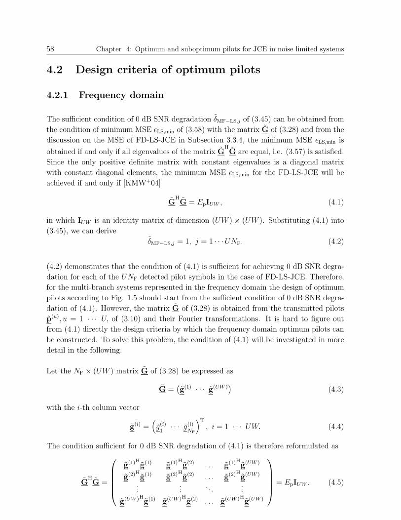
58 Chapter 4: Optimum and suboptimum pilots for JCE in noise limited systems
4.2 Design criteria of optimum pilots
4.2.1 Frequency domain
The sufficient condition of 0 dB SNR degradation δMF−LS,j of (3.45) can be obtained from
the condition of minimum MSE εLS,min of (3.58) with the matrix G of (3.28) and from the
discussion on the MSE of FD-LS-JCE in Subsection 3.3.4, the minimum MSE εLS,min is
obtained if and only if all eigenvalues of the matrix GHG are equal, i.e. (3.57) is satisfied.
Since the only positive definite matrix with constant eigenvalues is a diagonal matrix
with constant diagonal elements, the minimum MSE εLS,min for the FD-LS-JCE will be
achieved if and only if [KMW+04]
GHG = EpIUW , (4.1)
in which IUW is an identity matrix of dimension (UW ) × (UW ). Substituting (4.1) into
(3.45), we can derive
δMF−LS,j = 1, j = 1 · · ·UNF. (4.2)
(4.2) demonstrates that the condition of (4.1) is sufficient for achieving 0 dB SNR degra-
dation for each of the UNF detected pilot symbols in the case of FD-LS-JCE. Therefore,
for the multi-branch systems represented in the frequency domain the design of optimum
pilots according to Fig. 1.5 should start from the sufficient condition of 0 dB SNR degra-
dation of (4.1). However, the matrix G of (3.28) is obtained from the transmitted pilots
p(u), u = 1 · · · U, of (3.10) and their Fourier transformations. It is hard to figure out
from (4.1) directly the design criteria by which the frequency domain optimum pilots can
be constructed. To solve this problem, the condition of (4.1) will be investigated in more
detail in the following.
Let the NF × (UW ) matrix G of (3.28) be expressed as
G =(g(1) · · · g(UW )
)(4.3)
with the i-th column vector
g(i) =(
g(i)
1· · · g(i)
NF
)T
, i = 1 · · · UW. (4.4)
The condition sufficient for 0 dB SNR degradation of (4.1) is therefore reformulated as
GHG =
g(1)Hg(1) g(1)Hg(2) . . . g(1)Hg(UW )
g(2)Hg(1) g(2)Hg(2) . . . g(2)Hg(UW )
......
. . ....
g(UW )Hg(1) g(UW )Hg(2) . . . g(UW )Hg(UW )
= EpIUW . (4.5)

4.2 Design criteria of optimum pilots 59
(4.5) implies that in order to design the optimum pilots for the frequency domain multi-
branch systems, the two requirements
g(i)Hg(i) = Ep, i = 1 · · · UW, (4.6)
and
g(i1)Hg(i2) = 0, i1 = 1 · · · UW, i2 = 1 · · · UW, i1 6= i2 (4.7)
must be fulfilled. (4.6) and (4.7) represent, respectively, the properties of the auto-
correlation and the cross-correlation of the column vectors g(i), i = 1 · · ·UW , of (4.4)
of the matrix G of (3.28) with which the frequency domain optimum pilots can be ob-
tained.
The two requirements of (4.6) and (4.7) can be further analyzed in the following:
The matrix G of (3.28) can be expressed in detail as
G = P FW,tot =
p(1)
1p(1)
1. . . p(1)
1. . . p(U)
1. . . p(U)
1
p(1)
2p(1)
2e−j 2π
NF . . . p(1)
2e−j
2π(W−1)NF . . . p(U)
2. . . p(U)
2e−j
2π(W−1)NF
......
. . ....
. . ....
. . ....
p(1)
NFp(1)
NFe−j
2π(NF−1)
NF . . . p(1)
NFe−j
2π(NF−1)(W−1)
NF . . . p(U)
NF. . . p(U)
NFe−j
2π(NF−1)(W−1)
NF
︸︷︷︸
g(1)
︸︷︷︸
g(2)
. . .︸︷︷︸
g(W )
. . .︸︷︷︸
g((U−1)W+1)
︸︷︷︸
g(UW )
.
(4.8)
Considering the column vectors g(i), i = 1 · · ·UW, of the matrix G of (3.28), we obtain
the autocorrelation of the column vectors
g(i)Hg(i) =
NF∑
nF=1
p(u)
nF
∗p(u)
nF= p(u)Hp(u), i = 1 · · ·UW, U = 1 · · ·U,U = b i
Wc, (4.9)
in which b.c means to round the element to the nearest integer towards minus infinity.
(4.6) can be satisfied from (4.9) since (3.11) has been assumed, i.e. the pilot vectors
p(u), u = 1 · · ·U, of (3.10) on the U branches have the same energy Ep for transmission
as described in (3.11).
For the cross-correlation of the column vectors g(i) of (4.4) of matrix G, i.e. g(i1)Hg(i2),
i1 = 1 · · ·UW, i2 = 1 · · ·UW , i1 6= i2, from (4.8) we have
g(i1)Hg(i2) =
NF∑
nF=1
p(u1)
nF
∗p(u2)
nFe−j
2π(nF−1)(w2−w1)
NF ,
u1 = 1 · · ·U, u2 = 1 · · ·U,w1 = 1 · · ·W,w2 = 1 · · ·W, i1 6= i2,
u1 = b i1W
c, u2 = b i2W
c, w1 = mod(i1 − 1,W ), w2 = mod(i2 − 1,W ),
(4.10)
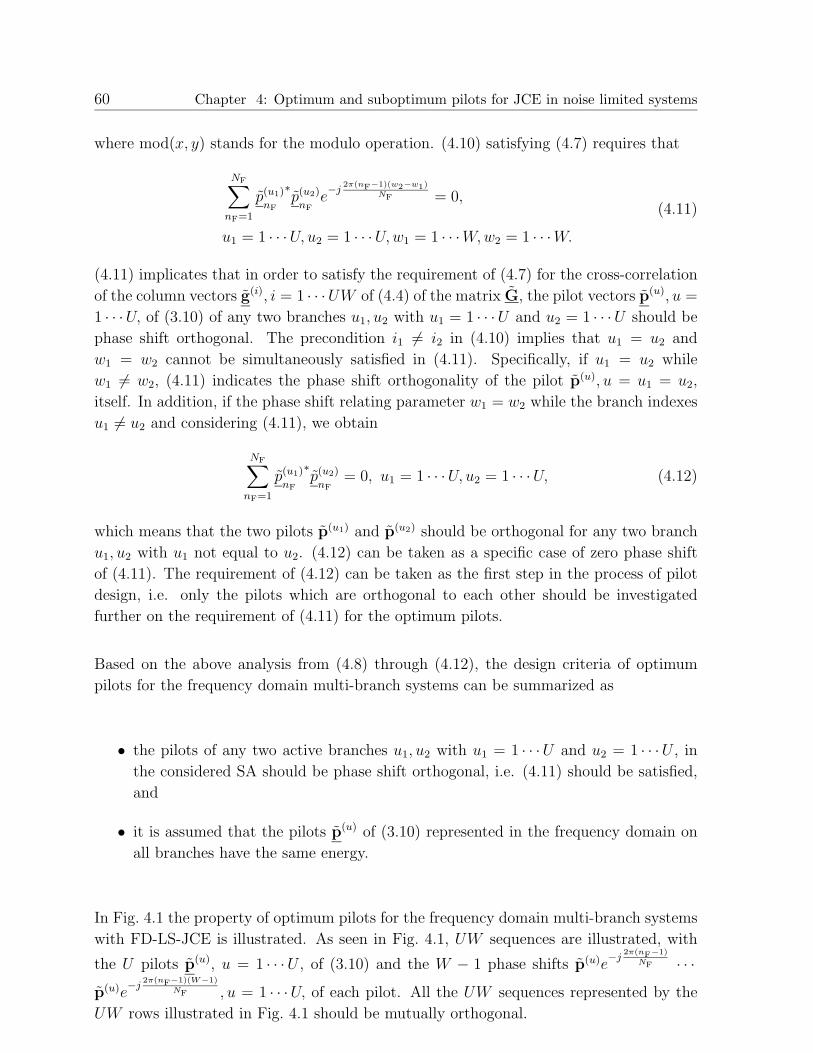
60 Chapter 4: Optimum and suboptimum pilots for JCE in noise limited systems
where mod(x, y) stands for the modulo operation. (4.10) satisfying (4.7) requires that
NF∑
nF=1
p(u1)
nF
∗p(u2)
nFe−j
2π(nF−1)(w2−w1)
NF = 0,
u1 = 1 · · ·U, u2 = 1 · · ·U,w1 = 1 · · ·W,w2 = 1 · · ·W.(4.11)
(4.11) implicates that in order to satisfy the requirement of (4.7) for the cross-correlation
of the column vectors g(i), i = 1 · · ·UW of (4.4) of the matrix G, the pilot vectors p(u), u =
1 · · ·U, of (3.10) of any two branches u1, u2 with u1 = 1 · · ·U and u2 = 1 · · ·U should be
phase shift orthogonal. The precondition i1 6= i2 in (4.10) implies that u1 = u2 and
w1 = w2 cannot be simultaneously satisfied in (4.11). Specifically, if u1 = u2 while
w1 6= w2, (4.11) indicates the phase shift orthogonality of the pilot p(u), u = u1 = u2,
itself. In addition, if the phase shift relating parameter w1 = w2 while the branch indexes
u1 6= u2 and considering (4.11), we obtain
NF∑
nF=1
p(u1)
nF
∗p(u2)
nF= 0, u1 = 1 · · ·U, u2 = 1 · · ·U, (4.12)
which means that the two pilots p(u1) and p(u2) should be orthogonal for any two branch
u1, u2 with u1 not equal to u2. (4.12) can be taken as a specific case of zero phase shift
of (4.11). The requirement of (4.12) can be taken as the first step in the process of pilot
design, i.e. only the pilots which are orthogonal to each other should be investigated
further on the requirement of (4.11) for the optimum pilots.
Based on the above analysis from (4.8) through (4.12), the design criteria of optimum
pilots for the frequency domain multi-branch systems can be summarized as
• the pilots of any two active branches u1, u2 with u1 = 1 · · ·U and u2 = 1 · · ·U , in
the considered SA should be phase shift orthogonal, i.e. (4.11) should be satisfied,
and
• it is assumed that the pilots p(u) of (3.10) represented in the frequency domain on
all branches have the same energy.
In Fig. 4.1 the property of optimum pilots for the frequency domain multi-branch systems
with FD-LS-JCE is illustrated. As seen in Fig. 4.1, UW sequences are illustrated, with
the U pilots p(u), u = 1 · · ·U , of (3.10) and the W − 1 phase shifts p(u)e−j
2π(nF−1)
NF · · ·p(u)e
−j2π(nF−1)(W−1)
NF , u = 1 · · ·U, of each pilot. All the UW sequences represented by the
UW rows illustrated in Fig. 4.1 should be mutually orthogonal.

4.2 Design criteria of optimum pilots 61
orthogonal
mutually
p(1)
1p(1)
2p(1)
NF
p(1)
1e−j
2π(nF−1)
NF p(1)
2e−j
2π(nF−1)
NF p(1)
NFe−j
2π(nF−1)
NF
p(1)
1e−j
2π(nF−1)(W−1)
NF p(1)
2e−j
2π(nF−1)(W−1)
NF p(1)
NFe−j
2π(nF−1)(W−1)
NF
p(U)
1p(U)
2p(U)
NF
p(U)
1e−j
2π(nF−1)
NF p(U)
2e−j
2π(nF−1)
NF p(U)
NFe−j
2π(nF−1)
NF
p(U)
1e−j
2π(nF−1)(W−1)
NF p(U)
2e−j
2π(nF−1)(W−1)
NF p(U)
NFe−j
2π(nF−1)(W−1)
NF
Fig. 4.1. Orthogonal property of the frequency domain optimum pilots.
4.2.2 Time domain
By considering the equivalence between the time domain and the frequency domain rep-
resentations of JCE in Section 3.4, we obtain from (3.71)
GHG = PH
FHF P = PHP. (4.13)
By substituting (4.13) into the condition of the frequency domain optimum pilots of (4.1),
we derive
PHP = EpIUW . (4.14)
Substituting (4.14) into (3.91), it follows for the SNR degradation
δMF−LS,j = 1, j = 1 · · ·UW, (4.15)
i.e. 0 dB SNR degradation for TD-LS-JCE can be obtained. That means, the condition of
(4.14) is sufficient for the time domain optimum pilots by which 0 dB SNR degradation can
be achieved. Therefore, the design of optimum pilots for the time domain multi-branch
systems should start from (4.14).
From (3.70), (4.14) can be equivalently expressed as
P(u)HP(u) = EpIW , u = 1 · · ·U, (4.16)

62 Chapter 4: Optimum and suboptimum pilots for JCE in noise limited systems
in which IW is an identity matrix of dimension W ×W , and
P(u1)HP(u2) = 0, u1 = 1 · · ·U, u2 = 1 · · ·U, u1 6= u2. (4.17)
Furthermore, from the structure of P(u) of (3.69), (4.16) is represented as
Lp∑
lp=1
p(u)
lp
∗p(u)
lp= Ep, u = 1 · · ·U, (4.18)
andLp∑
lp=1
p(u)
lp
∗p(u)
lp−w+1= 0, u = 1 · · ·U,w = 2 · · ·W. (4.19)
Hence, (4.17) is represented as
Lp∑
lp=1
p(u1)
lp
∗p(u2)
lp−w+1= 0, u1 = 1 · · ·U, u2 = 1 · · ·U, u1 6= u2, w = 1 · · ·W. (4.20)
Note that with the guard vector g(u) of (3.18) being composed of the cyclic shift of the
pilot vector p(u) of (3.1) as illustrated in Fig. 3.4, we have
p(u)
lp−w+1= p(u)
Lp+lp−w+1, if lp ≤ w − 1, u = 1 · · ·U,w = 1 · · ·W. (4.21)
(4.18) is satisfied if all the U branches use the same energy Ep for pilot transmission, i.e.
(3.11) is satisfied, which is assumed in the thesis. (4.19) and (4.20) require, respectively,
the shift orthogonal property of each pilot itself and between each pair of pilots. Therefore,
the design criteria of the time domain optimum pilots can be summarized as
• the pilots of any two active branches u1, u2 with u1 = 1 · · ·U and u2 = 1 · · ·U , in the
considered SA should be shift orthogonal, i.e. (4.19) and (4.20) should be satisfied,
and
• it is assumed that the pilots represented in the time domain on all branches have
the same energy.
The design criteria of the time domain optimum pilots can be illustrated in Fig. 4.2. In
order to make (4.19) and (4.20) satisfied, the UW sequences illustrated by the UW rows
in Fig. 4.2 should be mutually orthogonal.

4.2 Design criteria of optimum pilots 63
orthogonal
mutually
p(1)1
p(1)1
p(1)2
p(1)Lp−1
p(1)Lp−1
p(1)Lp−2
p(1)Lp−W
p(1)Lp−W+1
p(1)Lp−W+2
p(1)Lp−W+3
p(1)Lp
p(1)Lp
p(U)1
p(U)1
p(U)2
p(U)Lp−1
p(U)Lp−1
p(U)Lp−2
p(U)Lp−W
p(U)Lp−W+1
p(U)Lp−W+2
p(U)Lp−W+3
p(U)Lp
p(U)Lp
Fig. 4.2. Orthogonal property of the time domain optimum pilots.
4.2.3 Equivalence between the time and frequency domain de-
sign criteria of optimum pilots
In Section 3.4, the equivalence between the time and the frequency domain representations
of the multi-branch systems has been explained. Since based on (4.13), the condition of
the time domain optimum pilots of (4.14) can be obtained from the frequency domain
optimum pilots of (4.1), and vice verse, the design criteria of the time domain optimum
pilots of (4.19) and (4.20) is equivalent to the design criteria of the frequency domain
optimum pilots of (4.11).
The equivalence between the design criteria of the time domain optimum pilots and the
frequency domain optimum pilots implicates that we can design optimum pilots for the
multi-branch systems either in the time domain according to the design criteria of (4.19)
and (4.20) or in the frequency domain according to the design criteria of (4.11). By
considering the relationship of the time and the frequency domain pilots of (3.13), we can
conclude that the optimum pilots for the time domain multi-branch systems satisfying
(4.19) and (4.20), after DFT, will also be the optimum pilots for the frequency domain
multi-branch systems satisfying (4.11). Similarly, the optimum pilots for the frequency
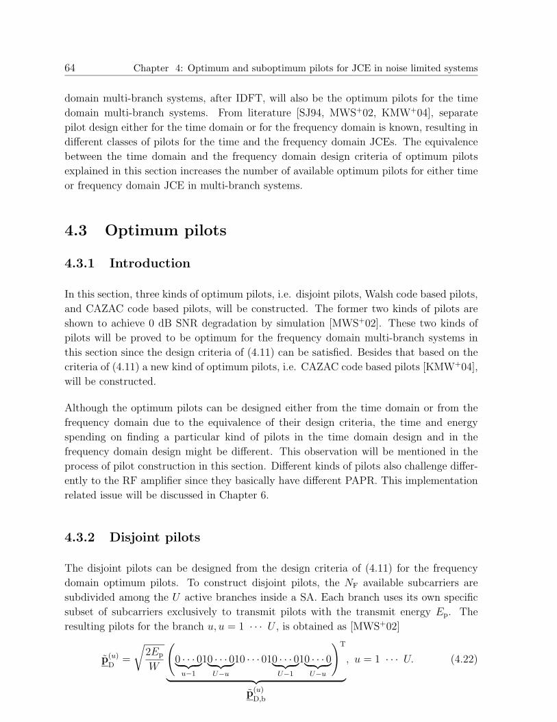
64 Chapter 4: Optimum and suboptimum pilots for JCE in noise limited systems
domain multi-branch systems, after IDFT, will also be the optimum pilots for the time
domain multi-branch systems. From literature [SJ94, MWS+02, KMW+04], separate
pilot design either for the time domain or for the frequency domain is known, resulting in
different classes of pilots for the time and the frequency domain JCEs. The equivalence
between the time domain and the frequency domain design criteria of optimum pilots
explained in this section increases the number of available optimum pilots for either time
or frequency domain JCE in multi-branch systems.
4.3 Optimum pilots
4.3.1 Introduction
In this section, three kinds of optimum pilots, i.e. disjoint pilots, Walsh code based pilots,
and CAZAC code based pilots, will be constructed. The former two kinds of pilots are
shown to achieve 0 dB SNR degradation by simulation [MWS+02]. These two kinds of
pilots will be proved to be optimum for the frequency domain multi-branch systems in
this section since the design criteria of (4.11) can be satisfied. Besides that based on the
criteria of (4.11) a new kind of optimum pilots, i.e. CAZAC code based pilots [KMW+04],
will be constructed.
Although the optimum pilots can be designed either from the time domain or from the
frequency domain due to the equivalence of their design criteria, the time and energy
spending on finding a particular kind of pilots in the time domain design and in the
frequency domain design might be different. This observation will be mentioned in the
process of pilot construction in this section. Different kinds of pilots also challenge differ-
ently to the RF amplifier since they basically have different PAPR. This implementation
related issue will be discussed in Chapter 6.
4.3.2 Disjoint pilots
The disjoint pilots can be designed from the design criteria of (4.11) for the frequency
domain optimum pilots. To construct disjoint pilots, the NF available subcarriers are
subdivided among the U active branches inside a SA. Each branch uses its own specific
subset of subcarriers exclusively to transmit pilots with the transmit energy Ep. The
resulting pilots for the branch u, u = 1 · · · U , is obtained as [MWS+02]
p(u)
D=
√
2Ep
W
(
0 · · · 0︸ ︷︷ ︸
u−1
10 · · · 0︸ ︷︷ ︸
U−u
10 · · · 010 · · · 0︸ ︷︷ ︸
U−1
10 · · · 0︸ ︷︷ ︸
U−u
)T
︸ ︷︷ ︸
p(u)
D,b
, u = 1 · · · U. (4.22)

4.3 Optimum pilots 65
The term√
2Ep
Win (4.22) is to guarantee the transmit energy of the disjoint pilots to be
Ep.
In a fully loaded system, the condition
NF = UW (4.23)
holds [SMW+01]. In an example case of NF = 16 subcarriers, U = 4 branches and
W = 4 channel coefficients, according to (4.22), the binary disjoint pilots p(u)
D,bwithout
considering the term√
2Ep
Wfor the U branches are constructed as
p(1)
D,b= (1000100010001000)T
p(2)
D,b= (0100010001000100)T
p(3)
D,b= (0010001000100010)T
p(4)
D,b= (0001000100010001)T
(4.24)
Since the U pilots are orthogonal but not shift orthogonal, the disjoint pilots of (4.22)
can only be designed from the two criteria (4.12) and (4.11) for the frequency domain
multi-branch systems. That means, the disjoint pilots of (4.22) cannot be applied directly
to the time domain multi-branch systems but have to resort to IDFT to obtain the time
domain optimum pilots.
The disadvantage when choosing optimum pilots according to (4.22) is that the resulting
set of pilots is the only possible set for the U branches in the considered SA. This means
that adjacent SAs, if only disjoint pilots are applied, must apply the same set of pilots so
that the interfering signals have similarities with the desired signals of the reference SA.
This will adversely influence their performance in interference environments, which will
be further discussed in Chapter 5.
4.3.3 Walsh code based pilots
The Walsh code based pilots can be designed from the frequency domain design criteria of
(4.11). To construct Walsh code based pilots of dimension NF, we consider a Hardamard
matrix
AW =
[H1 H1
H1 −H1
]
(4.25)
of dimensionNF×NF, in which H1 is a submatrix with dimension NF
2×NF
2. The Hardamard
matrix AW can be also represented as
AW =[w1 · · · wnF
· · · wNF
], nF = 1 · · · NF, (4.26)
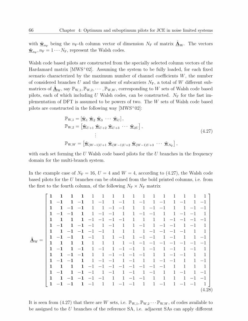
66 Chapter 4: Optimum and suboptimum pilots for JCE in noise limited systems
with wnFbeing the nF-th column vector of dimension NF of matrix AW. The vectors
wnF, nF = 1 · · ·NF, represent the Walsh codes.
Walsh code based pilots are constructed from the specially selected column vectors of the
Hardamard matrix [MWS+02]. Assuming the system to be fully loaded, for each fixed
scenario characterized by the maximum number of channel coefficients W , the number
of considered branches U and the number of subcarriers NF, a total of W different sub-
matrices of AW, say PW,1,PW,2, · · · ,PW,W , corresponding to W sets of Walsh code based
pilots, each of which including U Walsh codes, can be constructed. NF for the fast im-
plementation of DFT is assumed to be powers of two. The W sets of Walsh code based
pilots are constructed in the following way [MWS+02]:
PW,1 = [w1 w2 w3 · · · wU ] ,
PW,2 =[wU+1 wU+2 wU+3 · · · w2U
],
...
PW,W =[w(W−1)U+1 w(W−1)U+2 w(W−1)U+3 · · · wNF
],
(4.27)
with each set forming the U Walsh code based pilots for the U branches in the frequency
domain for the multi-branch system.
In the example case of NF = 16, U = 4 and W = 4, according to (4.27), the Walsh code
based pilots for the U branches can be obtained from the bold printed columns, i.e. from
the first to the fourth column, of the following NF ×NF matrix
AW =
1 1 1 1 1 1 1 1 1 1 1 1 1 1 1 11 −1 1 −1 1 −1 1 −1 1 −1 1 −1 1 −1 1 −11 1 −1 −1 1 1 −1 −1 1 1 −1 −1 1 1 −1 −11 −1 −1 1 1 −1 −1 1 1 −1 −1 1 1 −1 −1 11 1 1 1 −1 −1 −1 −1 1 1 1 1 −1 −1 −1 −11 −1 1 −1 −1 1 −1 1 1 −1 1 −1 −1 1 −1 11 1 −1 −1 −1 −1 1 1 1 1 −1 −1 −1 −1 1 11 −1 −1 1 −1 1 1 −1 1 −1 −1 1 −1 1 1 −11 1 1 1 1 1 1 1 −1 −1 −1 −1 −1 −1 −1 −11 −1 1 −1 1 −1 1 −1 −1 1 −1 1 −1 1 −1 11 1 −1 −1 1 1 −1 −1 −1 −1 1 1 −1 −1 1 11 −1 −1 1 1 −1 −1 1 −1 1 1 −1 −1 1 1 −11 1 1 1 −1 −1 −1 −1 −1 −1 −1 −1 1 1 1 11 −1 1 −1 −1 1 −1 1 −1 1 −1 1 1 −1 1 −11 1 −1 −1 −1 −1 1 1 −1 −1 1 1 1 1 −1 −11 −1 −1 1 −1 1 1 −1 −1 1 1 −1 1 −1 −1 1
(4.28)
It is seen from (4.27) that there are W sets, i.e. PW,1,PW,2 · · ·PW,W , of codes available to
be assigned to the U branches of the reference SA, i.e. adjacent SAs can apply different

4.3 Optimum pilots 67
sets of Walsh code based pilots, which allows perform JCE simultaneously using different
sets of Walsh code based pilots in different SAs, even in the case of a large number of
adjacent SAs.
The Walsh code based pilots are the frequency domain optimum pilots which satisfy
the frequency domain design criteria of (4.11), as proved in Section 4.3.5 [KMW+04].
However, since the columns of the Hardamard matrix are not shift orthogonal, they
cannot be constructed directly from the time domain design criterion of (4.14), However,
from the equivalence of the time and the frequency domain design criteria of optimum
pilots as described in Section 4.2.3, the Walsh code base pilots constructed as (4.27) will
become the optimum pilots for the time domain JCE after IDFT.
Restricted by the construction of a Hardamard matrix, the dimension of the Walsh code
based pilots NF must be power of two.
4.3.4 CAZAC code based pilots
In this subsection, a new kind of optimum pilots, CAZAC code based pilots, is proposed
and constructed. They are called CAZAC code based pilots because the pilots of the U
branches are all CAZAC codes [Hei61, FZH62, Chu72, BC02]. The CAZAC codes are
complex-valued pseudo-random noise (PN) sequences with constant amplitude assuming
values on the unit circle and with cyclic correlation functions equal to zero apart from
the only one peak at the starting point. For a CAZAC code
c =(c1 · · · cNF
)T(4.29)
of dimension NF with the property
ck+NF= ck, k = 0 · · ·NF − 1, (4.30)
its cyclic correlation vector
rc =(rc,1 · · · rc,NF
)T(4.31)
is obtained by determining the elements [Hei61]
rc,i =
NF−1∑
k=0
ck+ick∗, i = 1 · · ·NF. (4.32)
The CAZAC codes are also called polyphase sequences [FZH62, Chu72]. The application
of CAZAC codes alleviates the PAPR problem in OFDM systems [KMW+04], which will
be discussed in Chapter 6.
68 Chapter 4: Optimum and suboptimum pilots for JCE in noise limited systems
The CAZAC code based pilots can be constructed from the frequency domain design
criteria of (4.11). The CAZAC code c can be constructed in several ways, such as in
[Hei61] and [BC02]. According to [Hei61], the CAZAC code c is defined as follows:
If P is an integer number greater than one, there are P different roots of unity, i.e.
ξ0, ξ
1, · · · , ξ
P−1, with
ξk
= e−j(2πk/P ), 0 ≤ k ≤ P − 1. (4.33)
With the P roots of unity, a square matrix
C =
1 1 1 1 11 ξ
1ξ2
1· · · ξP−1
1
1 ξ2
ξ2
2· · · ξP−1
2...
......
. . ....
1 ξP−1
ξ2
P−1· · · ξP−1
P−1
. (4.34)
of dimension P × P is formed. The CAZAC code vector c of dimension NF = P 2 is then
generated by reading the matrix C of (4.34) column by column, i.e.
c = (111 · · · 11ξ1ξ
2ξ
3· · · ξ
P−11ξ2
1ξ2
2ξ2
3· · · ξ2
P−1· · · 1ξP−1
1ξP−1
2ξP−1
3· · · ξP−1
P−1)T. (4.35)
In [Hei61], P is required to be a prime number. However, it was later pointed out in
[FZH62] that P is not necessarily to be prime. With the generation of the CAZAC code
c according to (4.33) to (4.35), the dimension NF of the CAZAC code c is restricted to
the square of an integer.
However, with the construction of the CAZAC code vector c according to [BC02], the
restriction on the dimension NF of the CAZAC code vector c is diminished, i.e. the
dimension NF of the CAZAC code vector c could be any value. Let NF and M be two
integer numbers which are relatively prime. Hence, the elements cl+1, l = 0 · · ·NF − 1, of
the CAZAC code c of dimension NF according to [BC02] are derived as
cl+1 =
{
ej Mπl2
NF , l = 0 · · ·NF − 1, if NF is even
ej
Mπl(l+1)NF , l = 0 · · ·NF − 1, if NF is odd
(4.36)
Generally, for a certain dimension NF of the CAZAC code vector c there is more than
one number of M that is relatively prime to NF. Therefore, there is more than one
CAZAC code available based on the construction of the CAZAC code in [BC02]. Since
the dimension NF of Walsh code based pilots is limited to the power of two, CAZAC code
based pilots might be more attractive regarding application than Walsh code based pilots
in the case that the dimension of training sequences has to be flexible.
Taking the CAZAC code vector c of (4.29) as a mother CAZAC code, a NF ×NF matrix
AC =[c1 · · · cnF
· · · cNF
], nF = 1 · · · NF (4.37)

4.3 Optimum pilots 69
can be formed with the nF-th column
cnF=
[0 InF
INF−nF0
]
c, nF = 1 · · · NF (4.38)
being the CAZAC code vector cyclically shifted by nF − 1 symbols from c of (4.29).
From the matrix AC of (4.37), in the case of a fully loaded system, W submatrices
PC,1 =[c1 cW+1 c2W+1 · · · c(U−1)W+1
],
PC,2 =[c2 cW+2 c2W+2 · · · c(U−1)W+2
],
...
PC,W =[cW c2W c3W · · · cNF
]
(4.39)
can be constructed, with each submatrix PC,w, w = 1 · · ·W , of dimension NF × U con-
taining U columns of the matrix AC.
In (4.39), each column in a submatrix PC,w, w = 1 · · ·W , corresponds to the pilot of
one branch so that the U sequences in one submatrix correspond to the U pilots for the
frequency domain multiple branches in one SA. The pilots in the other submatrices can
be applied to the branches in the other SAs.
In an example case of NF = 16, U = 4 and W = 4, according to (4.39), the CAZAC code
based pilots for the U branches can be obtained as the bold printed columns, i.e. the
first, the fifth, the ninth and the thirteenth column of the matrix
AC =
1 j −1 −j 1 −1 1 −1 1 −j −1 j 1 1 1 11 1 j −1 −j 1 −1 1 −1 1 −j −1 j 1 1 11 1 1 j −1 −j 1 −1 1 −1 1 −j −1 j 1 11 1 1 1 j −1 −j 1 −1 1 −1 1 −j −1 j 11 1 1 1 1 j −1 −j 1 −1 1 −1 1 −j −1 jj 1 1 1 1 1 j −1 −j 1 −1 1 −1 1 −j −1
−1 j 1 1 1 1 1 j −1 −j 1 −1 1 −1 1 −j−j −1 j 1 1 1 1 1 j −1 −j 1 −1 1 −1 11 −j −1 j 1 1 1 1 1 j −1 −j 1 −1 1 −1
−1 1 −j −1 j 1 1 1 1 1 j −1 −j 1 −1 11 −1 1 −j −1 j 1 1 1 1 1 j −1 −j 1 −1
−1 1 −1 1 −j −1 j 1 1 1 1 1 j −1 −j 11 −1 1 −1 1 −j −1 j 1 1 1 1 1 j −1 −j
−j 1 −1 1 −1 1 −j −1 j 1 1 1 1 1 j −1−1 −j 1 −1 1 −1 1 −j −1 j 1 1 1 1 1 j
j −1 −j 1 −1 1 −1 1 −j −1 j 1 1 1 1 1
.
(4.40)
In (4.40), the mother CAZAC code vector c, i.e. the first column of matrix AC, the
elements whose amplitude is 1, is obtained according to [Hei61]. The real and imagery

70 Chapter 4: Optimum and suboptimum pilots for JCE in noise limited systems
1 3 5 7 9 11 13 15 17 19
0
5
10
15
20
1 3 5 7 9 11 13 15 17 19
0
5
10
15
20
Rea
lr c
,iIm
agr c
,i
i, i = 1 · · ·NF
Fig. 4.3. Cyclic autocorrelation of the mother CAZAC code in (4.40).
parts Real rc,i, i = 1 · · ·NF, and Imag rc,i, i = 1 · · ·NF, of the elements of the cyclic
correlation rc of (4.31) of this mother CAZAC code is illustrated in Fig. 4.3.
It is seen from (4.39) that there is more than one set of codes available to be assigned to
the U branches of the reference SA, i.e. adjacent SAs can apply different sets of CAZAC
code based pilots. Besides, it should be noted that the generation of the pilots according
to (4.39) is based on merely one mother CAZAC code c. Hence, more CAZAC code
based pilot resources can be assigned to the branches in all SAs than in the case of Walsh
code based pilots, since for a certain dimension NF there exists generally a certain amount
of CAZAC codes, where each of which could act as the mother CAZAC code c.
Furthermore, CAZAC code based pilots according to (4.39) are shift orthogonal since
they have the cyclic correlation properties as shown in Fig. 4.3, they can also be directly
constructed from the time domain design criteria of (4.14). This implies that the CAZAC
code based pilots constructed according to (4.39) can be applied to the time domain
multi-branch systems directly as the optimum pilots.

4.3 Optimum pilots 71
4.3.5 Proof of the optimum pilots
In this subsection, as an example, the Walsh code based pilots constructed according to
(4.27) will be proved to be optimum pilots. The disjoint pilots constructed according to
(4.22) and the CAZAC code based pilots constructed according to (4.39) can be verified
to be optimum pilots in the similar way. Consequently, this will not be elaborately proved
in this Subsection.
In the following, it is sufficient to prove that the design criterion of (4.11) can be fulfilled
by their construction of (4.27) since the Walsh code based pilots are designed directly for
the use in the frequency domain of multi-branch systems.
Since the column vectors of the Hardamard matrix of (4.26) are orthogonal, the pilots in
each set of (4.27) will fulfill the correlation property given in (4.12) under the condition
of w1 = w2. Therefore, in the following, it is to prove that Walsh code based pilots satisfy
the design criterion (4.11) under the condition of w1 6= w2.
In order to make (4.11) fulfilled, the equation
NF∑
nF=1
e−j
2π(nF−1)(w2−w1)
NF = 0, w1 = 1 · · · W,w2 = 1 · · · W,w1 6= w2, (4.41)
can be taken into account with the general assumption that NF is power of two. The
elements in the sum of (4.41) are distributed on the unit circle by exploiting the structure
of the Hardamard matrix and by considering that the sum of any two elements which are
symmetrical with respect to the center of the unit circle is equal to zero, we can prove
that Walsh code based pilots satisfy (4.11) in the following way:
From the structure of the Hardamard matrix AW of (4.25), it can be seen that in the case
of W > 1, i.e. W = 2, 4, 8, 16, · · · , with the construction of pilots according to (4.27),
p(u1)
nF1
∗p(u2)
nF1= p(u1)
nF2
∗p(u2)
nF2, ∀nF1, nF2 = 1 · · ·NF, |nF2 − nF1| =
NF
2,
u1 = 1 · · · U, u2 = 1 · · · U, u1 6= u2, w1 = 1 · · ·W, w2 = 1 · · ·W, w1 6= w2,(4.42)
is valid for any scenario with the given parameters NF, U , and W in fully loaded systems.
(4.42) implies that the two coefficients p(u1)
nF1
∗p(u2)
nF1and p(u1)
nF2
∗p(u2)
nF2in (4.11) in front of any two
elements in (4.41) which are symmetrical to the center of the unit circle, i.e. |nF2−nF1| =NF
2, are equal, which implies that
p(u1)
nF
∗p(u2)
nFe−j
2π(nF−1)(w2−w1)
NF + p
(u1
)
nF+NF2
∗
p
(u2
)
nF+NF2
e−j
2π(nF−1+NF2 )(w2−w1)
NF = 0
∀nF = 1 · · · NF
2, u1 = 1 · · ·U, u2 = 1 · · ·U, u1 6= u2, w1 = 1 · · ·W,w2 = 1 · · ·W,w1 6= w2.
(4.43)

72 Chapter 4: Optimum and suboptimum pilots for JCE in noise limited systems
(4.11) will be fulfilled by the summation over NF
2pairs, i.e. nF = 1 · · · NF
2, of (4.43).
Therefore, the construction of Walsh code based pilots of (4.27) in the case W > 1 will
fulfill (4.11). In the case of W = 1 we have w1 = w2 = 1. Then, the condition (4.11) is
reduced to (4.12), which can be fulfilled by the orthogonality of Walsh codes.
4.4 Suboptimum pilots
The suboptimum pilots refer to those by which neither the time domain design criterion
of (4.14) nor the frequency domain design criterion of (4.11) of optimum pilots can be
fulfilled.
The easiest way to generate suboptimum pilots is to use random pilots [MWS+02]. Ran-
dom pilots are randomly generated with elements from the set −1, 1. Random pilots are
used in [MWS+02, KMW+04] and also in Chapter 7 of this thesis for the performance
comparison with the optimum pilots, i.e. disjoint pilots, Walsh code based pilots and
CAZAC code based pilots. In addition, a lot of other sequences can be used as the sub-
optimum pilots without the restriction of the optimum JCE performance in terms of 0
dB SNR degradation.
Basically, the time domain design criterion of (4.14) and the frequency domain design
criterion of (4.11) call for sequences with ideal autocorrelation and cross-correlation char-
acteristics, i.e. the sequences involved in Fig. 4.2 or Fig. 4.1 should be mutually or-
thogonal. The following families of codes, which do not have ideal autocorrelation and
cross-correlation, are suboptimum pilots:
• maximum-length sequences (or m-sequences), which are generated using simple lin-
ear feedback shift register [BC02]. m-sequences have unideal but good autocorrela-
tion characteristic [BC02].
• gold sequences, which are first proposed in [Gol67]. They are generated from m-
sequences and can provide a large number of codes with the same correlation. Gold
sequences have good autocorrelation and cross-correlation characteristics [BC02].
• Kasami sequences, which have good cross-correlation properties [Pro95].
• orthogonal Gold sequences, which result from simple modifications of Gold sequences
and can provide zero cross-correlation at certain points [DJ98].
Furthermore, with the recent application of space-time block codes [Ala98] with two
antennas to the WCDMA [WCDMA], some pilots are proposed for channel estimation.
4.5 Numerical results of SNR degradations 73
For example, the two pilots
p(1) = (−1 − 111 − 1 − 1 − 11 − 1 − 1 − 1 − 1 − 1 − 111)T,p(2) = (−1 − 111111 − 1 − 1 − 1 − 1111 − 11)T (4.44)
are proposed for the two antennas as the recommended pilots of dimension 16 [WCDMA].
These two pilots p(1) and p(2) are orthogonal. However, they are not shift orthogonal or
phase shift orthogonal so that they are suboptimum pilots.
In addition, the pilots obtained by the exhaustive search in [SJ94] for the multiuser CDMA
systems are also suboptimum.
4.5 Numerical results of SNR degradations
The numerical results of the SNR degradations δMF−LS,j, j = 1 · · ·UNF, of (3.45) of the
optimum pilots, i.e. disjoint pilots, Walsh code based pilots and CAZAC code based
pilots, as well as of the suboptimum pilots such as random pilots will be shown in this
section. The exemplary scenario with NF = 64, U = 16, and W = 4 is adopted. Disjoint
pilots, Walsh code based pilots and CAZAC code based pilots are constructed according
to (4.22), (4.27) and (4.39), respectively. As for the CAZAC code based pilots, the mother
CAZAC code c is constructed as in (4.33) through (4.35).
The aforementioned pilots are first applied to the multi-branch system represented in the
frequency domain. In Fig. 4.4, the SNR degradations δMF−LS,j of (3.45), j = 1 · · ·UNF, of
the four classes of pilots for the FD-LS-JCE are plotted versus the index j, j = 1 · · ·UNF,
whereas no interference from the neighboring SAs is assumed. It can be observed in Fig.
4.4 that the SNR degradations δMF−LS,j have high values if random pilots are applied,
while for disjoint pilots, Walsh code based pilots and CAZAC code based pilots, the SNR
degradations are 0 dB, which confirms the theoretical analysis of the previous sections.
In the following evaluation, the aforementioned pilots are applied to the time domain
multi-branch systems after the IDFT of these pilots. In Fig. 4.5, the SNR degradations
δMF−LS,j, j = 1 · · ·UW, of (3.91) for the TD-LS-JCE of the resulted four kinds of pilots are
shown. It is observed that the pilots obtained from the IDFT of the disjoint pilots, Walsh
code based pilots and CAZAC code based pilots still result in 0 dB SNR degradations.
This verifies the discussions of the equivalence between the time and frequency domain
design criteria of optimum pilots in Subsection 4.2.3.
In addition, as discussed in Subsection 4.3.4, the CAZAC code based pilots designed in
Subsection 4.3.4 can be directly applied to the time domain multi-branch systems because
they fulfill also the time domain design criterion of (4.14). Fig. 4.6 shows the SNR

74 Chapter 4: Optimum and suboptimum pilots for JCE in noise limited systems
0 200 400 600 800 1000 1200−5
0
5
10
15
20
25
30
35
40
random pilots
disjoint pilots Walsh code based pilots
CAZAC code based pilots
δ MF−
LS,j/d
B
j = 1 · · ·UNF
Fig. 4.4. SNR degradations δMF−LS,j, j = 1 · · ·UNF, in dB for the exemplary scenario ofNF = 64, U = 16 and W = 4. Random pilots, disjoint pilots, Walsh code basedpilots and CAZAC code based pilots are directly applied to the frequency domainmulti-branch system.
0 10 20 30 40 50 60 70−5
0
5
10
15
20
25
30
35
pilots obtained from the IDFT of disjoint pilots, Walsh code based pilots and CAZAC code based pilots
pilots obtained from the IDFT of random pilots
δ MF−
LS,j/d
B
j = 1 · · ·UW
Fig. 4.5. SNR degradation δMF−LS,j, j = 1 · · ·UW , in dB for the exemplary scenario of NF =64, U = 16 and W = 4. Random pilots, disjoint pilots, Walsh code based pilots andCAZAC code based pilots, after IDFT, are applied to the time domain multi-branchsystem.
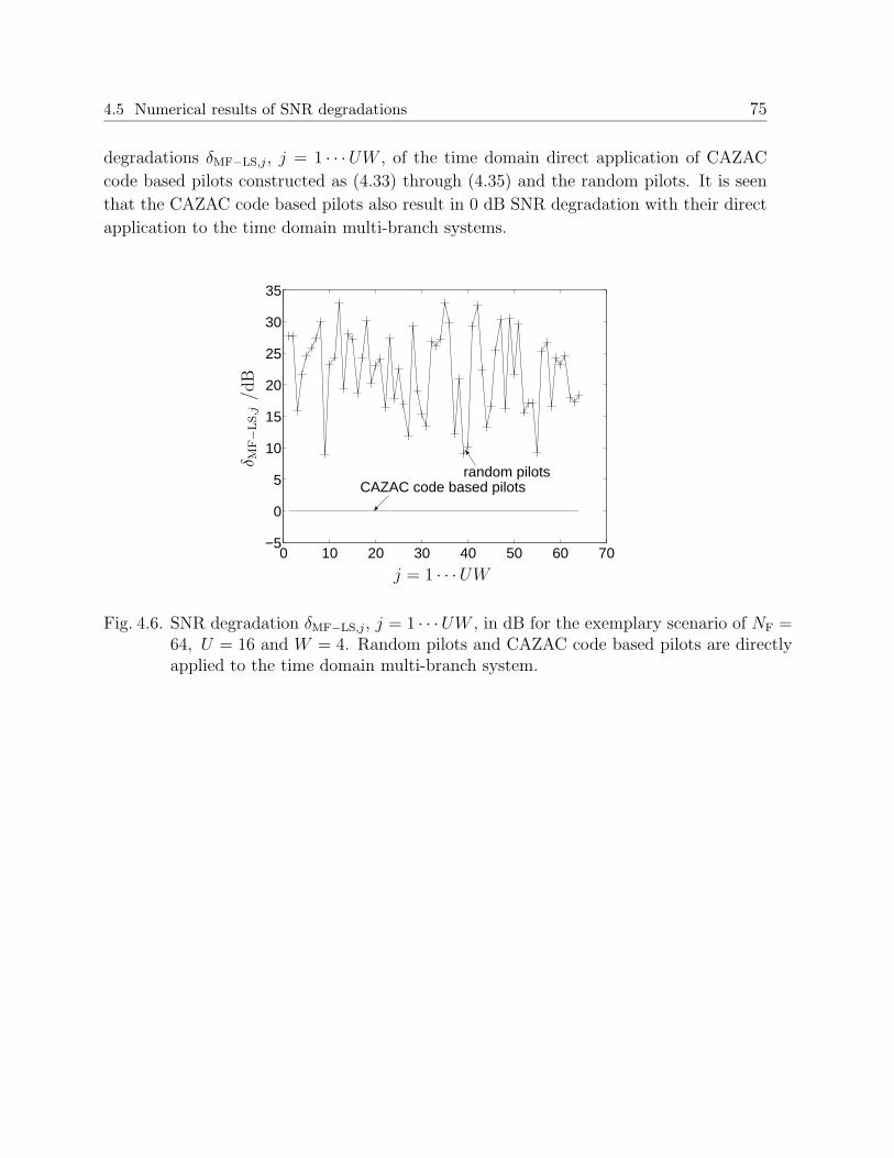
4.5 Numerical results of SNR degradations 75
degradations δMF−LS,j, j = 1 · · ·UW , of the time domain direct application of CAZAC
code based pilots constructed as (4.33) through (4.35) and the random pilots. It is seen
that the CAZAC code based pilots also result in 0 dB SNR degradation with their direct
application to the time domain multi-branch systems.
0 10 20 30 40 50 60 70−5
0
5
10
15
20
25
30
35
CAZAC code based pilots random pilots
δ MF−
LS,j/d
B
j = 1 · · ·UW
Fig. 4.6. SNR degradation δMF−LS,j, j = 1 · · ·UW , in dB for the exemplary scenario of NF =64, U = 16 and W = 4. Random pilots and CAZAC code based pilots are directlyapplied to the time domain multi-branch system.

76 Chapter 5: Pilot assignment in multiple SA environments
5 Pilot assignment in multiple SA environ-
ments
5.1 Introduction
In Chapter 4, the pilots for the multiple branches are designed according to the SNR
degradation evaluation in noisy environments by considering only one SA in the system.
Optimum and suboptimum pilots have been constructed for the time and the frequency
domain multi-branch systems. The sets of optimum pilots are disjoint pilots, Walsh code
based pilots and CAZAC code based pilots.
In practical mobile radio systems, however, the interference from neighboring SAs is
inevitable, which will adversely influence the capacity of the whole system. In the JOINT
concept [WMS+02], JCE is applied to estimate the channels of the U MTs simultaneously
in the considered SA and the MTs in other SAs appear to be interferers to the MTs in the
considered SA. In Subsection 3.3.5, the performance of JCE in interference environments
is evaluated by the variation coefficient, which, from its definition of (3.68), is influenced
by the pilots used in the considered SA and its neighboring SAs. Therefore, it is a big
challenge to the system designers to assign pilots to both the considered SA and the
neighboring SAs so that the overall system performance can be improved.
The problem of pilot assignment in multiple SA environments is illustrated in Fig. 5.1.
As an example, three SAs, SA1, SA2 and SA3, are shown, with three families of pilots,
pilot family 1, pilot family 2 and pilot family 3 which are assigned to the MTs in each
of the three SAs. Within each SA, the pilots for the multiple branches can be designed
according to the investigations in Chapter 4, i.e. if 0 dB SNR degradation is required,
the disjoint pilots, the Walsh code based pilots or the CAZAC code based pilots can be
applied. However, we have to face with the question that if, for example, SA1 uses the
Walsh code based pilots, should the same kind or the different kinds of pilots be selected
for SA1, SA2 and SA3?
In this chapter the issue of pilot assignment for the multiple SA scenarios will be investi-
gated. First, in Section 5.2 and Section 5.3, the scenario of two SAs, one reference SA and
one neighboring SA, with one single discrete strong interfering signal originating from the
adjacent SA, according to the interference model description in Section 2.5, will be con-
sidered. The variation coefficient discussed in Subsection 3.3.5 will be used to evaluate the
performance in this scenario. If, instead, there are lots of interferers from the neighboring
SAs and the signals from all the interferers are statistically independent and uniformly
distributed, the pdf of the sum of the interfering signals will be Gaussian according to the
central limit theorem [Pro95]. Thereby, the optimum pilots designed in Chapter 4 for one

5.2 Pilot assignment problem in interference environments 77
SA3
pilot family 2
pilot family 1
MT
pilot family 3
SA1
SA2
Fig. 5.1. Example of pilot assignment in multiple SAs/interference environments.
single SA in noisy environments will still be the optimum pilots no matter which kinds of
optimum pilots are used in the adjacent SAs.
As an example, the frequency domain representation of JCE of Section 3.3 will be con-
sidered in each SA. By considering the equivalence between the time and the frequency
domain representations of JCE which is discussed in Subsection 3.4.2, the conclusion
obtained in this chapter applies also to the time domain multi-branch systems.
Finally, in Section 5.4, the pilot assignment schemes for multi-SA scenarios will be pro-
posed based on the simulation results in Section 5.3.
5.2 Pilot assignment problem in interference envi-
ronments
It is observed from (3.64) that the JCE error in interference environments depends on
• the correlation properties of the pilots applied to the reference SA characterized by
PHP with the pilot matrix P according to (3.25),

78 Chapter 5: Pilot assignment in multiple SA environments
• the correlation properties of the pilots applied to the reference SA and the neighbor-
ing SA characterized by PHPI with the pilot matrix P of (3.25) and the interfering
pilot matrix PI of (3.60) of the neighboring SA, and
• the radio channel hI of (3.61) between the interferer in the neighboring SA and the
receiver in the considered AP.
In the case that the pilots in the reference SA are selected from the optimum pilots, such
as disjoint pilots, Walsh code based pilots and CAZAC code based pilots, the sufficient
condition of 0 dB SNR degradation of (4.5) will be fulfilled. Substituting (4.5) into the
JCE error of (3.64) in multiple SA environment, the JCE error of (3.64) in this case will
depend merely on the the correlation properties of the pilots applied to the reference SA
and to the adjacent SA characterized by PHPI, and on the interfering radio channel hI.
The design freedom for the good variation coefficient performance then lies in the pilots
used in the reference SA embraced in P of (3.25) and the pilot used in the neighboring
SA embraced in PI of (3.60).
In particular, the pilots used in the considered SA are chosen among the optimum pilots
of disjoint pilots, Walsh code based pilots and CAZAC code based pilots. While the pilot
used in the neighboring SA is chosen from one of these three kinds of pilots. Basically,
we have the following three options:
1. the interfering pilot is selected as one of the U pilots in the reference SA. Disjoint
pilots, Walsh code based pilots and CAZAC code based pilots can be applied to this
arrangement.
2. the interfering pilot is different from the U pilots in the reference SA. Nevertheless,
it is described from the same kind of pilots as the U pilots in the reference SA. In
this case, more pilot resource is required than the option 1. Walsh code based pilots
and CAZAC code based pilots can be applied to this arrangement. For CAZAC
code based pilots, the pilots in the reference SA and the pilot in the neighboring SA
use the same mother CAZAC code.
3. the interfering pilot and the U pilots in the reference SA come from different kinds
of pilots. For example, if disjoint pilots are used for the reference SA, then either
one pilot from Walsh code based pilots or from CAZAC code based pilots can be
used in the neighboring SA. The case that the pilots in the reference SA and its
neighboring SA use different mother CAZAC codes is also within this option.
The variation coefficient performance for above three options of pilots will be illustrated
in the next section. The variation coefficient vc of (3.68) describes how uniformly the
5.3 Variation coefficient simulation 79
interference power is distributed over the subcarriers of multiple branches in the reference
SA. The more uniformly the interference spreading over all subcarriers of all branches,
the smaller the variation coefficient. In the scenario of using all subcarriers for pilot
transmission for both the MTs in the considered SA and the strong interferer from the
neighboring SA, the ideal case of uniformly distributed interference power means that
the interference signal from the neighboring SA looks like white Gaussian noise to the
receiver in the reference SA. The random nature of the random pilots, when applied as
the interfering pilot and the U pilots in the reference SA, makes the interfering pilot
signal more like white Gaussian noise than the other pilots. Therefore, the random pilots
discussed in Section 4.4 will be taken as the reference in the variation coefficient evaluation
of various assignments of pilots.
5.3 Variation coefficient simulation
In this section, the variation coefficient performance with the three options for the pi-
lot selection described in Section 5.2 will be demonstrated. Since random channels are
considered in the simulation, the variation coefficient is a random variable. Therefore,
the cumulative distribution function (cdf) of the variation coefficient vc of (3.68) can be
plotted. The exemplary scenario of NF = 64, U = 16 and W = 4 is adopted in the
simulations.
In the first case, the simulation results of the pdfs of the variation coefficient are shown in
Fig. 5.2 according to option 1 in Section 5.2. Disjoint pilots, Walsh code based pilots and
CAZAC code based pilots are considered and the random pilots are taken as the reference.
For the disjoint pilots, as pointed out in Subsection 4.3.2, the U disjoint pilots constructed
as (4.22) are the only possibility of disjoint pilots. The interfering pilot is obtained as the
first one of the disjoint pilots derived by u = 1 according to (4.22). For the Walsh code
based pilots, the pilots of the U branches in the reference SA are obtained from the first
submatrix PW,1 of (4.27) and the interfering pilot is obtained from the first column vector
w1 in this submatrix. As for the CAZAC code based pilots, the pilots of the U branches
and the interfering pilot are obtained from the first submatrix PC,1 of (4.39) and the first
column vector c1 in this submatrix, respectively. For the random pilots, both the U pilots
in the reference SA and the interfering pilot are randomly selected. The random pilots
have the same energy Ep as disjoint pilots, Walsh code based pilots and CAZAC code
based pilots.
The x-axis V in Fig. 5.2 represents the threshold level of the variation coefficient, and
the y-axis represents cdf of the variation coefficient, i.e. the probability of the logarithm
of the variation coefficient vc not exceeding the threshold V , i.e. Prob{10lg10vc ≤ V }. It
is seen in Fig. 5.2 that with the arrangement of pilots according to option 1 in Section

80 Chapter 5: Pilot assignment in multiple SA environments
5.2, the variation coefficient performances of disjoint pilot, Walsh code based pilots and
CAZAC code based pilots are very close since the interfering pilot is the same with one of
the U pilots in the reference SA in these cases. For a certain variation coefficient threshold
V , the probability of the logarithm variation coefficient vc not exceeding the threshold V
for random pilots is much greater than the other three assignments of pilots. Therefore,
the random pilots will produce better performance than the other three assignments of
pilots in the system level.
−1 0 1 2 3 4 5 6 7 8 910
−3
10−2
10−1
100
random pilots
disjoint pilots
Walsh code based pilots
CAZAC code based pilots
Pro
b{1
0lg
10v c
≤V}
V /dB
Fig. 5.2. Cdf of the variation coefficient vc for the exemplary scenario of NF = 64,U = 16 and W = 4 according to option 1.
In the second case, the simulation results of the cdfs of the variation coefficients based
on the pilots arranged according to option 2 in Section 5.2 are demonstrated in Fig. 5.3.
Walsh code based pilots and CAZAC code based pilots are applied and random pilots are
used as the reference. For the Walsh code based pilots, the pilots of the U branches in
the reference SA are obtained from the first submatrix PW,1 in (4.27) and the interfering
pilot is selected as the first column vector wU+1 of the second submatrix PW,2 in (4.27).
For the CAZAC code based pilots, the pilots of the U branches in the reference SA and
the interfering pilot are obtained from the the first submatrix PC,1 and the first column
vector c2 of the second submatrix PC,2 in (4.39), respectively.
It is observed that the performance of Walsh code based pilots and CAZAC code based
pilots in the arrangement of pilots according to option 2 in Section 5.2 are close to each
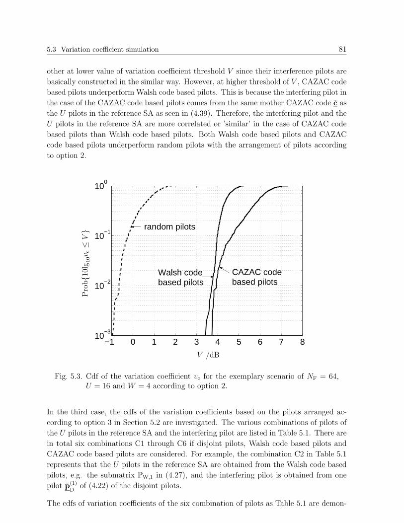
5.3 Variation coefficient simulation 81
other at lower value of variation coefficient threshold V since their interference pilots are
basically constructed in the similar way. However, at higher threshold of V , CAZAC code
based pilots underperform Walsh code based pilots. This is because the interfering pilot in
the case of the CAZAC code based pilots comes from the same mother CAZAC code c as
the U pilots in the reference SA as seen in (4.39). Therefore, the interfering pilot and the
U pilots in the reference SA are more correlated or ’similar’ in the case of CAZAC code
based pilots than Walsh code based pilots. Both Walsh code based pilots and CAZAC
code based pilots underperform random pilots with the arrangement of pilots according
to option 2.
−1 0 1 2 3 4 5 6 7 810
−3
10−2
10−1
100
random pilots
Walsh code based pilots
CAZAC code based pilots
Pro
b{1
0lg
10v c
≤V}
V /dB
Fig. 5.3. Cdf of the variation coefficient vc for the exemplary scenario of NF = 64,U = 16 and W = 4 according to option 2.
In the third case, the cdfs of the variation coefficients based on the pilots arranged ac-
cording to option 3 in Section 5.2 are investigated. The various combinations of pilots of
the U pilots in the reference SA and the interfering pilot are listed in Table 5.1. There are
in total six combinations C1 through C6 if disjoint pilots, Walsh code based pilots and
CAZAC code based pilots are considered. For example, the combination C2 in Table 5.1
represents that the U pilots in the reference SA are obtained from the Walsh code based
pilots, e.g. the submatrix PW,1 in (4.27), and the interfering pilot is obtained from one
pilot p(1)
Dof (4.22) of the disjoint pilots.
The cdfs of variation coefficients of the six combination of pilots as Table 5.1 are demon-

82 Chapter 5: Pilot assignment in multiple SA environments
Table 5.1. Various combination of pilots.
Combinationindex
The U pilots P in the refer-ence SA
The interfering pilot PI
C1 disjoint pilots of (4.22) a Walsh code w1 in (4.27)
C2 Walsh code based pilotsPW,1 in (4.27)
a disjoint pilot p(1)
Dof (4.22)
C3 Walsh code based pilotsPW,1 in (4.27)
a CAZAC code obtainedfrom [Hei61]
C4 CAZAC code based pilotsPC,1 in (4.39) whose motherCAZAC code comes from[Hei61]
a Walsh code w1 in (4.27)
C5 disjoint pilots of (4.22) a CAZAC code obtainedfrom [Hei61]
C6 CAZAC code based pilotsPC,1 in (4.39) whose motherCAZAC code comes from[Hei61]
a disjoint pilot p(1)
Dof (4.22)
strated in Fig. 5.4. It is seen in Fig. 5.4 that the six combinations of pilots, C1 through
C6, in Table 5.1 result in a variation coefficient performance which is comparable to the
random pilots. In particular, the third combination C3 of the Walsh code based pilots
PW,1 in (4.27) applied to the U branches in the reference SA and a pilot c1 in (4.39)
from the CAZAC code based pilots considered as the interfering pilot shows the best
performance.
Furthermore, as stated in Subsection 4.3.4, for CAZAC code based pilots, the mother
CAZAC code can be obtained from several methods, such as from [Hei61] whose generation
is given by (4.33) through (4.35) and from [BC02] whose generation is given by (4.36).
Even for one generation method of CAZAC codes, i.e. [BC02], for a certain dimension NF
of the pilots, more than one CAZAC code can be generated with the different choice M
in (4.36), each of which can serve as a mother code in the construction of CAZAC code
based pilots of (4.39). With different mother CAZAC codes, different CAZAC code based
pilots of (4.39) can be obtained. The case of using different CAZAC code based pilots
in different SAs is taken as the special case of option 3 in Section 5.2. In Table 5.2, the
three combinations CA1 to CA3 of pilots based on different mother CAZAC code based
pilots for the U pilots in the reference SA and the interfering pilot in the neighboring SA
are listed. In the first combination CA1, the U pilots in the reference SA are obtained
from the CAZAC code based pilots PC,1 in (4.39) whose mother CAZAC code is generated
from [Hei61] as (4.33) through (4.35), while the interfering pilot is generated from [BC02]

5.3 Variation coefficient simulation 83
−1.5 −1 −0.5 0 0.5 1 1.5 2 2.510
−3
10−2
10−1
100
random pilots C3 C6
C4
C2
C5
C1
Pro
b{1
0lg
10v c
≤V}
V /dB
Fig. 5.4. Cdf of the variation coefficient vc for the exemplary scenario of NF = 64,U = 16 and W = 4 according to option 3 (see also Table 5.1).
with M = 3 in (4.36). In the second combination CA2, the U pilots in the reference SA
are obtained from the CAZAC code based pilots PC,1 in (4.39) whose mother CAZAC
code comes from [BC02] with M = 3 in (4.36), while the interfering pilot is obtained from
[Hei61] as (4.33) through (4.35). In the third combination CA3, both the mother code of
the U pilots for the reference SA and the interfering pilot are obtained from [BC02] as
(4.36). However, they come from two different mother CAZAC codes with M = 3 and
M = 7, respectively.
In Fig. 5.5 the cdfs of variation coefficient of the three combinations of pilots CA1, CA2
and CA3 of Table 5.2 are simulated. It is observed in Fig. 5.5 that all of the three
combinations of CAZAC code based pilots produce the variation coefficient performance
much better than the random pilots. For example, the combination of CA3 results the
variation coefficient performance 4.4 dB better than the random pilots at the probability
level of 10−2. Comparing Fig 5.5 with Fig. 5.4, it is seen that the variation coefficient
performance of the three combinations CA1 to CA3 of Table 5.2 is also better than the
combinations C1 to C6 of Table 5.1. The simulation results of Fig. 5.5 encourages the
use of CAZAC code based pilots with different mother codes to different SAs.

84 Chapter 5: Pilot assignment in multiple SA environments
Table 5.2. Two combination of pilots based on CAZAC codebased pilots.
Combinationindex
The U pilots P for the ref-erence SA
The interfering pilot PI
CA1 CAZAC code based pilotsPC,1 in (4.39), whose motherCAZAC code comes from[Hei61]
a CAZAC code obtainedfrom [BC02] with M = 3
CA2 CAZAC code based pilotsPC,1 in (4.39), whose motherCAZAC code comes from[BC02] with M = 3
a CAZAC code obtainedfrom [Hei61]
CA3 CAZAC code based pilotsPC,1 in (4.39), whose motherCAZAC code comes from[BC02] with M = 3
a CAZAC code obtainedfrom [BC02] with M = 7
−8 −6 −4 −2 0 2 410
−3
10−2
10−1
100
CA3 CA2 CA1 random pilots
Pro
b{1
0lg
10v c
≤V}
V /dB
Fig. 5.5. Cdf of the variation coefficient vc for the exemplary scenario of NF = 64,U = 16 and W = 4 according to option 3 (see also Table 5.2).

5.4 Proposals of pilot assignment for multiple SAs 85
5.4 Proposals of pilot assignment for multiple SAs
Comparing the curves in Fig. 5.4 and Fig. 5.5 with Fig. 5.2 and Fig. 5.3, it can be
observed that the variation coefficient performance in the cases that different kinds of
pilots, as in Table 5.1 or in Table 5.2, are applied to the reference SA and its neighboring
SA will be much better than in the cases that the same kind of pilots, as the options 1
and 2 in Section 5.2, are applied to the different SAs.
The scenario of multiple SAs is the extension of the scenario of two SAs. Therefore,
the observation in Section 5.3 based on the simulation results applies to the scenario of
multiple SA also.
Based on the simulation results in Fig. 5.4, one scheme of pilot assignment is proposed in
Fig. 5.6 providing one possible solution of a pilot assignment that could be beneficial from
the interference point of view to the challenge of pilot assignment illustrated in Fig. 5.1.
Basically, as shown in Fig. 5.6, different kinds of optimum pilots from the disjoint pilots,
the Walsh code based pilots and the CAZAC code based pilots are assigned to different
SAs. For example, if disjoint pilots are assigned to the U branches in the reference SA1, the
CAZAC code based pilots and the Walsh code based pilots will be applied to the adjacent
SA2 and SA3, respectively. Fig. 5.6 illustrates the basic cluster of pilot assignment, which
can be extended physically by reusing the certain kind of pilots in the far SAs. With the
pilot assignment as in Fig. 5.6, the U pilots for each SA are the optimum pilots with 0 dB
SNR degradation, and the interference power with this arrangement of different kinds of
pilots to different SAs fluctuates less than the other pilot arrangements of options 1 and 3
in Section 5.2, which makes the behavior of interference more similar to white noise. This
will produce better channel estimation quality in multiple SA environment. Hence, less
bit error rate (BER) can be expected. Or equivalently say, more users can be transmitted
for a certain BER level. Therefore, the pilot assignment as proposed in Fig. 5.6 is expected
to increase the system capacity than the other arrangements of options 1 and 3 in Section
5.2 when system level simulation is investigated.
However, as will be elaborately discussed in Chapter 6, the disjoint pilots and the Walsh
code based pilots have worse PAPR performance than the CAZAC code based pilots [KMW+04].
So the former two kinds of pilots challenges the hardware implementation of the system.
By considering this issue, another scheme of pilot assignment is proposed in Fig. 5.7,
which is inspired by the simulation results in Fig. 5.5. Three different mother CAZAC
codes are chosen in the three SAs, resulting CAZAC code based pilots 1, CAZAC based
pilots 2 and CAZAC code based pilots 3 assigned to the multiple branches in SA1, SA2,
and SA3, respectively. The advantages with the assignment of pilots as in Fig. 5.7 are
• the pilots in each SA are the optimum pilots by which 0 dB SNR degradation can
be obtained,

86 Chapter 5: Pilot assignment in multiple SA environments
Walsh code based pilots
SA1
SA3
SA2
MT
CAZAC code based pilots
disjoint pilots
Fig. 5.6. The first proposal on the allocation of pilots to the multiple SAs.
• the interference power fluctuates slightly so that the good system performance can
be expected,
• the PAPR problem is alleviated in each SA.
It is of particular interest with the arrangement of pilots as Fig. 5.7 in the scenario that
more than three SAs are adjacent to the considered SA. In this scenario, since for a certain
dimension NF of pilots, there are normally amount of CAZAC code based pilots available
with different mother CAZAC codes, the arrangement of pilots as indicated by Fig. 5.7
will be directly derivable. However, if the arrangement of pilots as indicated by Fig. 5.6
is taken, then some new kinds of optimum pilots apart from the disjoint pilots, Walsh
code based pilots and CAZAC code based pilots have to be found and constructed in this
scenario.
As discussed in Subsection 4.2.3, the equivalence between the time domain and the fre-
quency domain design criteria of optimum pilots explained in this section increases the
number of available optimum pilots for either time or frequency domain JCE in multi-
branch systems. The increase of available optimum pilots raises the potential to assign
different pilots to different SAs, therefore, to improve the overall system performance for
both time and frequency domain multi-branch systems in multiple SA environments.

5.4 Proposals of pilot assignment for multiple SAs 87
For CAZAC code based pilots 1, 2 and 3, three different mother CAZAC codes are chosen
SA1
SA2
SA3
CAZAC code based pilots 1
MT
CAZAC code based pilots 2
CAZAC code based pilots 3
Fig. 5.7. The second proposal on the allocation of pilots to the multiple SAs.
88 Chapter 6: Application of JCE in OFDM and FMT based multi-branch systems
6 Application of JCE in OFDM and FMT
based multi-branch systems
6.1 Introduction
Despite the equivalence regarding time and frequency domain representations as discussed
in Section 3.4, the JCE technique has practically developed into the time and frequency
domain applications due to some implementation considerations concerning the implemen-
tation complexity and the PAPR. In this chapter, two application issues will be investi-
gated concerning the JCE technique as well the pilots. The first investigation addresses
the complexity evaluation of the TD-JCE and FD-JCE, based on which the choice of pro-
cessing JCE in the time domain or the frequency domain according to the complexity will
be made. The second investigation addresses the evaluation of PAPR of various pilots,
which is critical, if the efficiency of the radio frequency (RF) power amplifier is taken into
account.
In Section 6.2, the OFDM and FMT multi-carrier transmissions will be shortly introduced.
In Section 6.3, the choice of either time or frequency domain JCE for OFDM and FMT
systems will be discussed according to the evaluation of the processing complexity of
the TD-LS-JCE and the FD-LS-JCE. The PAPR issue will be discussed in Section 6.4
especially for OFDM systems. A general discussion on the applications of various optimum
pilots proposed in Section 4.3, i.e. disjoint pilots, Walsh code based pilots and CAZAC
code based pilots, follows in Section 6.5 according to the performance of these pilots in a
noisy environment, in an interference environment as well as to their PAPR properties.
6.2 Multi-carrier systems
6.2.1 Introduction
The application scenarios for JCE considered in this thesis are OFDM and FMT based
multi-carrier multi-branch systems. Before discussing the suitability of either the time
or the frequency domain JCE to OFDM and FMT based systems, which is carried out
in the following Section 6.3, the well known OFDM and FMT multi-carrier modulation
schemes will be briefly recapitulated in this section.
Both OFDM and FMT belong to the general family of filter bank multi-carrier (FB-MC)
modulation systems, in which parallel data streams are filtered by interpolating filters
with proper spectrum characteristics. If all the filters are frequency-shifted versions of

6.2 Multi-carrier systems 89
one prototype filter and the sub-carriers are equally spaced, then the FB-MC scheme can
be efficiently implemented through a bank of prototype filters and FFT [BC02, Fil04].
The general FB-MC modulation will be described in Subsection 6.2.2, with a general
model illustrated for the FB-MC modulation. Both the OFDM and the FMT modulated
multi-carrier transmission can be depicted by this general model, which will be discussed in
Subsections 6.2.3 and 6.2.4, respectively. Ideally the selected prototype filter in the general
model should be well localized in both the time and frequency domains to guarantee the
complete elimination of ISI and ICI [Bol99].
6.2.2 FB-MC modulation
Fig. 6.1 depicts the discrete time model of the general FB-MC modulation scheme. NF
represents the number of subcarriers, T denotes the multi-carrier symbol duration, i.e.
the time separation between two consecutive data symbols transmitted on one subcarrier.
F represents the subcarrier spacing. In this scheme the parallel data streams a0(lT )
through aNF−1(lT ) are upsampled by a factor Q to produce the transmit signals with
symbol rate Q/T . The resulting signals are then filtered by the same transmit prototype
filter c0(lT/Q) and are then allocated in the proper frequency region by the modulation
ej2π(0)FlT/Q through ej2π(NF−1)FlT/Q on each subcarrier.
With the subcarrier spacing
F =Q
NFT, (6.1)
and with reference to Fig. 6.1, the transmitted signal
x(lT
Q) =
NF−1∑
nF=0
+∞∑
n=0
anF(nT )c0[(l − nQ)
T
Q]e
j2πnFQ
TNF(l T
Q), l = 0 · · · + ∞ (6.2)
is obtained. From (6.2) it may be observed that each data symbol anF(nT ) is associated
with a signature
cnF((l − nQ)
T
Q) = c0[(l − nQ)
T
Q]e
j2πnFQ
TNF(l T
Q), l = 0 · · · + ∞, n = 0 · · · + ∞. (6.3)
The received signal y(lT/Q) is obtained as the convolution of the transmitted signal x(l TQ
)
of (6.2) and the CIR h(τ, lT/Q) corrupted by the AWGN noise n(l TQ
), i.e.
y(lT/Q) =+∞∑
τ=0
x(lT
Q− τ)h(τ, l
T
Q) + n(l
T
Q), l = 0 · · · + ∞. (6.4)
At the receiver, the receive signal y(lT/Q) is first demodulated by the multiplication with
e−j2π(nF−1)FlT/Q, nF = 1 · · ·NF, on each subcarrier, and then passed through a bank of

90 Chapter 6: Application of JCE in OFDM and FMT based multi-branch systems
a0(lT )
aNF−1(lT )
T
T
T
T
Q
Q
Q
Q
T/Q
T/Q
T/Q
T/Q
T/Q
c0(lT/Q)
c0(lT/Q)
ej2π(0)FlT/Q
ej2π(NF−1)FlT/Q
s1(lT/Q)
sNF(lT/Q)
x(lT/Q)
h(τ, t)
n(lT/Q)
y(lT/Q)e−j2π(0)FlT/Q
e−j2π(NF−1)FlT/Q
c∗0(−lT/Q)
c∗0(−lT/Q)
a0(lT )
aNF−1(lT )
Fig. 6.1. The discrete time model of the general FB-MC modulation scheme.
receive prototype filter c∗0(−lT/Q). The receive prototype filter c∗0(−lT/Q) is matched to
the transmit prototype filter c0(lT/Q). The resulting signal is then down sampled by the
factor Q to obtain the signal with the transmission rate 1/T . The receive symbols a0(lT )
through aNF−1(lT ) are expected to be further processed to improve the performance of
the system.
6.2.3 OFDM modulation
With Q = NF, the system is critically sampled [BC02]. This is the case for OFDM
systems. In this case, by inverting the sums and letting
lT
NF
= mT + iT
NF
, m = 0 · · · + ∞, i = 0 · · ·NF − 1, (6.5)

6.2 Multi-carrier systems 91
(6.2) can be represented as [Fil04]
x(mT+iT
NF
) =+∞∑
n=0
NF−1∑
nF=0
anF(nT )e
j2πinFNF c0(mT+i
T
NF
−nT ), m = 0 · · ·+∞, i = 0 · · ·NF−1,
(6.6)
in which the second sum is the IDFT of the transmit symbols, i.e.
Ai(nT ) =
NF−1∑
nF=0
anF(nT )e
j2πinFNF = IDFT[anF
(nT )]. (6.7)
By substituting (6.7) into (6.6), it reads as
x(mT + iT
NF
) =+∞∑
n=0
Ai(nT )c0(mT + iT
NF
− nT ), m = 0 · · · + ∞, i = 0 · · ·NF − 1. (6.8)
With (6.8), the complexity of implementing the general FB-MC system illustrated in
Fig. 6.1 is reduced significantly thanks to the use of the IDFT operation, which can
be carried out via the FFT algorithm. The complexity can be further reduced by the
polyphase decomposition which eliminates the multiplications by zero introduced by the
upsampling operation [BC02].
In the OFDM system, the transmit prototype filter c0(lT/Q) in Fig. 6.1 is chosen to have
rectangular shape in the time domain, i.e.
c0(lT/Q) =
{1 0 ≤ l ≤ NF − 10 elsewhere
(6.9)
With (6.9) and with 0 ≤ i ≤ M − 1, the elements of the sum in (6.8) are not zero only
for n = m, so that (6.8) can be reduced to
x(mT + iT
NF
) = Ai(mT ), m = 0 · · · + ∞, i = 0 · · ·NF − 1, (6.10)
which is obtained by the IDFT of the input data stream.
Fig. 6.2 illustrates the frequency spectrum of an OFDM system with the exemplary case
of Q = 16 and NF = 16. The x-axis fT represents the normalized frequency band with
respect to the subcarrier spacing F , which is the inverse of symbol duration T in the
OFDM system. The y-axis 20log10(|C(f)|) /dB represents the amplitude of the spectrum
in dB.

92 Chapter 6: Application of JCE in OFDM and FMT based multi-branch systems
0 2 4 6 8 10 12 14 16−30
−25
−20
−15
−10
−5
0
5
fT
20lo
g10(|C
(f)|)
/dB
Fig. 6.2. Frequency spectrum in an OFDM system with the exemplary case of Q = 16and NF = 16.
6.2.4 FMT modulation
In the general FB-MC scheme illustrated in Fig. 6.1, with Q > NF, the system is not
critically sampled [BC02], which is the case in FMT systems. In this case, with every NF
input samples Q output samples are obtained. Therefore, a redundancy related to the
factor Q/NF is introduced. An excess bandwidth is introduced that allows the transition
region of the prototype filter to be enlarged of a factor of α = Q/NF.
In Fig. 6.3 it is shown that a part of the bandwidth is used for the transition region of the
prototype filter [Fil04]. With such an approach ICI is significantly reduced since ideally,
ff0 f1 = QNFT
f2 = 2QNFT
1/T
QNFT
Fig. 6.3. Not critically sampling in FMT systems.
6.2 Multi-carrier systems 93
i.e. with infinitive length of the prototype filter, there is no crossover among adjacent
carriers.
In the following, m = 0 · · · + ∞ and i = 0 · · ·NF − 1 are assumed. In the not critically
sampled case with Q > NF, by letting
lT
NF
= (mNF + i)T
NF
, (6.11)
(6.2) can be represented as [Fil04]
x(mNFT
Q+ i
T
Q) =
+∞∑
n=0
NF−1∑
nF=0
anF(nT )e
j2πnFQ
TNF(mNF
TQ
+i TQ
)c0[(mNF + i− nQ)
T
Q]. (6.12)
By considering (6.7), (6.12) can be rewritten as
x(mNFT
Q+ i
T
Q) =
+∞∑
n=0
Ai(nT )c0(mNFT
Q+ i
T
Q− nTQ). (6.13)
With (6.13), the complexity of implementing the not critically sampled FB-MC system
is reduced by FFT algorithm. The complexity can be further reduced by polyphase
decomposition [CEO02].
In the FMT system, the prototype filter c0(lT/Q) is chosen to have a well localized shape
in the frequency domain. Hence, by means of not critically sampling, it may be guaranteed
that no overlapping (in the ideal case of the prototype filter with unlimited length) or
almost no overlapping (in the practical case the prototype filter with limited length by
windowing) occurs between adjacent sub-carriers. For example, the almost no overlapping
condition may be fulfilled by windowing the prototype filter of a root raised cosine (rrcos)
with roll-off factor ρ ≤ α, which is given by [Fil04]
√
rcos(x, α) =
1 for 0 ≤ |x| ≤ 1−α2,
cos(π2
|x|− 1−α2
α) for 1−α
2< |x| ≤ 1+α
2,
0 for |x| > 1+α2.
(6.14)
Fig. 6.4 depicts the frequency spectrum in the case of rrcos with ρ = 0.15 for the not
critically sampling with Q = 18 and NF = 16. The x-axis fNFT/Q represents the
normalized frequency band with respect to the subcarrier spacing F , which is given by
Q/(NFT ) in the FMT system. The y-axis 20log10(|C(f)|) /dB represents the amplitude
of the spectrum in dB. The high spectral containment of FMT systems as seen in Fig.6.4
makes them particularly robust to time and frequency synchronization offsets. This is
achieved with the expense of bandwidth efficiency by introducing frequency redundancy.

94 Chapter 6: Application of JCE in OFDM and FMT based multi-branch systems
0 2 4 6 8 10 12 14 16−50
−40
−30
−20
−10
0
fNFT/Q
20lo
g10(|C
(f)|)
/dB
Fig. 6.4. Frequency spectrum of the square-root raised cosine prototype filter withthe roll-off factor of 0.15 in the case of Q = 18, NF = 16 in the FMT system.
6.3 Time versus frequency domain JCE for OFDM
and FMT systems
In this section, the choice of either time or frequency domain JCE according to their
processing complexity for OFDM and FMT systems is considered. For this reason, the
processing complexity for implementing the TD-LS-JCE and the FD-LS-JCE is firstly
evaluated and compared. Lp = NF is assumed in the evaluation.
With the time domain receive signal vector r of dimension Lp, see (3.81), and with the
time domain total pilot matrix P of (3.70) of dimension Lp × (UW ), the TD-LS-JCE
estimate hLS of the total CIR h of (2.28) is obtained according to (3.86). From (3.86),
the process of the TD-LS-JCE can be decomposed into the two steps of matched filtering
and sidelobe cancellation filter [FB92] as shown in Fig. 6.5. The matched filtering on the
receive signal vector r results the TD-MF-JCE hMF of (3.85). The sidelobe filtering of
hMF yields the TD-LS-JCE hLS of (3.86).
With the frequency domain receive signal vector r of dimension NF, see (3.28), and with
the matrix G of (3.28) of dimension NF×(UW ), the FD-LS-JCE estimate ˆhLS of the total
CTF h of (3.20) is obtained according to (3.40). From (3.40), the process of the FD-LS-
JCE can be decomposed into the three steps of matched filtering, sidelobe cancellation
filter and the Fourier transformation as shown in Fig. 6.6. Matched filtering of the receive

6.3 Time versus frequency domain JCE for OFDM and FMT systems 95
filtermatched filter sidelobe cancellation
rPH
hMF(PHP)−1
hLS
Fig. 6.5. Decomposition of the TD-LS-JCE.
signal vector r yields the FD-MF-JCE estimate hMF of (3.32) on the total CIR h of (2.28).
The sidelobe filtering of hMF results in the FD-LS-JCE estimate hLS of (3.34) of the total
CIR h of (2.28). The Fourier transformation of hLS results in the FD-LS-JCE estimateˆhLS of the total CTF h of (3.20).
matched filter sidelobe cancellation
filter
Fourier Transform
rG
hMF hLS(
GHG)−1
FW,tot
ˆhLS
Fig. 6.6. Decomposition of the FD-LS-JCE.
As discussed in Subsections 4.2.1 and 4.2.2, with the optimum pilots used in the frequency
and the time domain multi-branch transmissions, (4.14) and (4.1) can be fulfilled, respec-
tively. Therefore, the inversion operation (PHP)−1 in the structure shown in Fig. 6.5
and the inversion operation (GHG)−1 in the structure shown in Fig. 6.6 will have the
same complexity and both scale the estimate hMF by a factor 1/Ep. Even if suboptimum
pilots are considered by taking into account the expression of (4.13), these two inversion
operations still have the same complexity. Therefore, for comparing the complexity of
TD-LS-JCE and FD-LS-JCE, the two inversion operations (PHP)−1 and (GHG)−1 are
omitted, i.e. only the complexity of the TD-MF-JCE of (3.85) of the total CIR h and the
complexity of FD-MF-JCE of (3.39) of the total CTF h will be considered. Particularly,
in the following the number of complex multiplications and FFTs (IFFTs) in (3.85) and
(3.39) will be calculated.
For the TD-MF-JCE of (3.85), the number
ηCMT= UWLp (6.15)
of complex multiplications corresponding to the first step, i.e. the matched filtering, in
the structure shown in Fig. 6.5 is required.

96 Chapter 6: Application of JCE in OFDM and FMT based multi-branch systems
For the FD-MF-JCE of (3.39), by considering the definition of matrix G in (3.28), its
complexity evaluation can be more clearly seen from Fig. 6.7.
rP F
H
W,totFW,tot
ˆhMF
Fig. 6.7. Decomposition of the FD-MF-JCE.
From the discussion in Section 3.2, the three matrices in Fig. 6.7 P, FH
W,tot and FW,tot
should be a-priori known to the receiver. Therefore, the total matrix FW,totFH
W,totP
of dimension (UNF) × NF is also a-priori known, which can be calculated off-line. A
direct calculation of the complexity of the structure shown in Fig. 6.7 is based on the
multiplication of the total matrix FW,totFH
W,totP with the receive signal vector r. The
number of complex multiplications
ηCMF= UN2
F (6.16)
is obtained in this direct calculation.
As discussed in Subsection 3.3.1, the number W of channel coefficients is typically smaller
than the number NF of subcarriers in OFDM systems [NP00]. Generally, NF is at least
4 to 10 times larger than W [FAB02]. One reason for this is to minimize the fraction of
overhead due to the insertion of the cyclic prefix at the beginning of each transmission
block. When comparing (6.16) with (6.15), it is observed that the number of complex
multiplications ηCMTof (6.15) for the TD-MF-JCE is always smaller than the number of
complex multiplications ηCM1Fof (6.16) for the FD-MF-JCE under the assumption that
Lp = NF.
However, the complexity of FD-MF-JCE can be reduced by the fast implementation of
the Fourier transformation. Generally, the NF-point DFT can be fastly implemented by
NF-point FFT with NFlog2(NF) complex multiplications [BC02]. The first block in the
structure shown in Fig. 6.7 brings UNF complex multiplications, while the second and
the third blocks in Fig. 6.7 in total require 2U NF-point FFTs, each of which has NF
inputs, while only W outputs are useful for the FD-MF-JCE. Hence, the total number of
complex multiplications for the FD-MF-JCE in the structure shown in Fig. 6.7 is
ηCMF= UNF + 2UNFlog2(NF). (6.17)
From (6.15) and (6.17), with the same number of U branches in both the time and
the frequency domain multi-branch transmissions, and under the assumption that Lp =

6.3 Time versus frequency domain JCE for OFDM and FMT systems 97
NF, the complexity of TD-MF-JCE and FD-MF-JCE is related to the number NF of
subcarriers or the dimension Lp of the pilots as well as the number of channel coefficients
W . It is derived from (6.15) and (6.17) that in the case
W > 1 + 2log2(NF) (6.18)
the complexity of TD-MF-JCE of (6.15) is greater than the complexity of FD-MF-JCE
of (6.17). Therefore, the FD-LS-JCE should be chosen according to the complexity eval-
uation. In contrast to this, in the case
W < 1 + 2log2(NF) (6.19)
the complexity of the TD-MF-JCE of (6.15) is less than the complexity of FD-MF-JCE
of (6.17). Therefore, the TD-LS-JCE should be chosen according to the complexity eval-
uation.
From (6.18) and (6.19), the choice of TD-LS-JCE or FD-LS-JCE according to their com-
plexity evaluation is illustrated in Fig. 6.8. The horizontal axis represents the dimension
NF of the frequency domain pilot or the dimension Lp of the time domain pilot. The
vertical axis represents the number W of channel coefficients. The curve in Fig. 6.8 illus-
trates the function 1 + 2log2(NF) as in (6.18) and (6.19). Therefore, if the implementing
complexity is the critical factor in choosing either the TD-LS-JCE or the FD-LS-JCE, the
range above the curve in Fig. 6.8 corresponding to the case that (6.18) can be satisfied
represents the scenario in which FD-LS-JCE should be selected. In contrast to this, the
range below the curve in Fig. 6.8 corresponding to the case that (6.19) can be satisfied
represents the scenario in which TD-LS-JCE should be selected. Since the number of
branches U influences the complexity of both the TD-LS-JCE which is reduced to (6.15)
in the case of optimum pilots and the FD-LS-JCE which is reduced to (6.17) in the case
of optimum pilots linearly, Fig. 6.8 is valid for the systems with any number of branches.
Based on above discussions, the choice of the processing domain of JCE for OFDM and
FMT based multi-branch multi-carrier systems can be discussed according to the com-
plexity evaluation of JCE.
The dominant propagation impairment of multipath in broadband wireless access systems
causes multiple echoes of the transmitted signal to be received with excess delays of up
to tens of microseconds [EMG99]. For symbol rates in the range of tens of megabits per
second, this translates to intersymbol interference that can span up to 100 or more data
symbols [FAB02]. For the parameters of beyond 3G systems given in Table 2.1, the symbol
rate of 20 MHz and the maximum excess delay of 5 µs in the worse scenario of outdoor
mean that W = 100 channel coefficients can be resolved if we sample with the symbol rate
at the receiver. If, e.g. there are 512 subcarriers in the considered multi-branch OFDM
system, the FD-LS-JCE should be used [SWB02, MWS+02] according to Fig. 6.8 with
respect to obtain low complexity.

98 Chapter 6: Application of JCE in OFDM and FMT based multi-branch systems
0 100 200 300 400 500 6000
2
4
6
8
10
12
14
16
18
20
FD-LS-JCE
TD-LS-JCE
W
NF = Lp
1 + 2log2(NF)
Fig. 6.8. The choice of TD-LS-JCE and FD-LS-JCE according to the complexity.
As for the FMT systems, with the appropriately designed prototype filter, the ICI between
the subchannels in FMT systems is negligible [BC02], as demonstrated in Fig. 6.4 as an
example. Therefore, the signal processing, e.g. the JCE, at the receiver is normally
carried out subcarrier wise [BTT02, KWC04a]. With the total symbol rate of 20 MHz
over the broadband channel, by considering, e.g. 16 subcarriers in the FMT system, the
5 µs excess delay in the worse case of outdoor given in Table 2.1 means that about W = 6
channel taps can be resolved, if we sample with the symbol rate on each subcarrier at
the receiver. Therefore, according to Fig. 6.8, for the pilot dimension Lp e.g. around 30,
it is more preferable to adopt TD-LS-JCE on each subcarrier with respect to obtain low
complexity [KWC04a].
6.4 PAPR issue in OFDM systems
6.4.1 General
In wireless communication systems, the RF transmitter dominates power consumption and
heat generation at the MT and at the BS or AP [SG01]. The PAPR of the transmitted
waveform determines the bias point and efficiency of the transmit power amplifier. For
a given required power output, the greater the PAPR, the greater the required power
amplifier back-off, and, therefore, the lower the amplifier efficiency. Hence, the PAPR
issue should be considered in the signal processing such as in the channel estimation.

6.4 PAPR issue in OFDM systems 99
It is found out that the PAPR in a single carrier system, in which the signals are processed
and transmitted in the time domain, is 4.5 to 5 dB lower than that in an OFDM system,
in which the signals are first allocated in the frequency domain and then transformed
into the time domain by IFFT for transmission, with 256 or 512 subcarriers using QPSK
modulation [SG01]. That means that the signals transmitted in OFDM systems are more
crucial with respect to the PAPR problem. Therefore, the discussion on the PAPR issue
will be restricted to the frequency domain channel estimation in this section. Particularly,
the PAPR issue will be investigated for the three optimum pilots, namely disjoint pilots,
Walsh code based pilots and CAZAC code based pilots proposed in Section 4.3.
6.4.2 PAPR comparison of various pilots
Based on the fact that the time domain pilot symbol p(u,lp), u = 1 · · ·U, lp = 1 · · · lp, in
(3.1) presents in the physical transmission models as shown in Fig. 1.4 and Fig. 1.5, from
(3.1), by assuming Lp = NF, the discrete time PAPR
η(u) =
maxnF∈(1,NF)
|p(u,nF)|2
E{|p(u,nF)|2} , u = 1 · · · U, (6.20)
for the u-th branch is derived [MH97, WNW01]. The PAPR η(u) of (6.20) is the square
of the crest factor [MH97].
The optimum pilots of disjoint pilots, Walsh code based pilots and CAZAC code based
pilots in Section 4.3 are designed and expressed in the frequency domain. From (3.13),
the time domain expression of the pilot on the u-th branch
p(u) = F−1
p(u), u = 1 · · · U, (6.21)
can be obtained, i.e. the time domain expression of the pilot on the u-th branch is the
IDFT of the frequency domain expression of the pilot on the u-th branch.
The numerical results of the power of one snapshot of the time domain expression of the
disjoint, Walsh and CAZAC pilots, i.e. |p(u,nF)|2, nF = 1 · · · NF, of one branch u versus the
time discrete point nF is shown in Fig. 6.9. The exemplary scenario of NF = 64, U = 16
and W = 4 is considered. The x-axis in Fig. 6.9 represents NF time discrete points of the
time domain expression of these pilots, and the y-axis represents the power of these pilots
over these discrete points. It is observed that apart from the CAZAC pilot, the other two
pilots exhibit time-variant power. Among disjoint pilot, Walsh pilot and CAZAC pilot,
Walsh pilot has the highest peak power, while CAZAC pilot has the lowest power and
uniform power distribution over the NF discrete time points. This tendency of different
pilots holds also for the other branches.

100 Chapter 6: Application of JCE in OFDM and FMT based multi-branch systems
0 10 20 30 40 50 60 700
0.05
0.1
0.15
0.2
0.25
0.3
0.35
0.4
0.45disjoint pilotWalsh pilotCAZAC pilot
|p(u
,nF) |2
nF
Fig. 6.9. The power of the time domain pilot sequence |p(u,nF)|2, u = 1 · · ·U, nF =1 · · ·NF, for the exemplary scenario of NF = 64, U = 16 and W = 4.
To evaluate the PAPR, the U branch specific PAPRs of (6.20) are averaged. The averaged
PAPR
η =1
U
U∑
u=1
η(u) (6.22)
in dB is shown in Table 6.1. Also the exemplary scenario of NF = 64, U = 16 and W = 4
is considered. It is observed in Table 6.1 that among the disjoint pilots, the Walsh code
based pilots and the CAZAC code based pilots, the Walsh code based pilots have the
highest average PAPR, which is 14.7882 dB. The average PAPR of the disjoint pilots
is in between while the PAPR of the CAZAC code based pilots is 0 dB. That means,
comparing with disjoint pilots and Walsh code based pilots, CAZAC code based pilots
alleviate the problem of PAPR in OFDM based systems greatly. It would be challenging
to the hardware, such as A/D, D/A converters and RF power amplifier, if, e.g. Walsh
code based pilots are applied directly to multi-user OFDM systems for JCE.
Table 6.1. Averaged PAPR of different pilots.
Pilots Averaged PAPR /dB
Disjoint pilots 6.0206Walsh code based pilots 14.7882
CAZAC code based pilots 0

6.5 Applications of various optimum pilots 101
6.5 Applications of various optimum pilots
In this section, some general discussions on the three kinds of optimum pilots in Section
4.3, i.e. disjoint pilots, Walsh code based pilots and CAZAC code based pilots will be
made for their applications in multi-branch multi-carrier systems.
Up to now, the presented three kinds of optimum pilots have been investigated in three
aspects, i.e. their performance in terms of SNR degradation in noisy environments as
in Section 4.5, their performance in interference environments in terms of variation co-
efficient as in Section 5.3, as well as their implementation issue concerning PAPR in
Subsection 6.4.2. As seen in Section 4.5, in noisy environments, disjoint pilots, Walsh
code based pilots and CAZAC code based pilots have the same performance in terms of
SNR degradation. In interference environments, as seen in Fig. 5.4, the choice of using
different kinds of pilots, i.e. disjoint pilots, Walsh code based pilots and CAZAC code
based pilots, to different SAs appears to have good variation coefficient performance.
However, by considering the PAPR performance of various pilots, it would be challenging
to the RF front end if Walsh code based pilots are used in one of the SAs. The choice
of using CAZAC code based pilots, but with different mother CAZAC code to different
SAs, will produce not only the best variation coefficient performance, as seen in Fig. 5.5,
but also the ideal PAPR performance in each SA. Therefore, with this arrangement of
pilots, the best solution of pilots in terms of the best performance in noise and interference
environments, as well as of the best PAPR performance, can be obtained.
The performance advantage of CAZAC code based pilots is obtained at the price of higher
hardware requirement. Since CAZAC code based pilots are normally composed of non-
binary elements, they require more memory than Walsh code based pilots, which consist
of binary elements. However, this disadvantage of CAZAC code based pilots could be
balanced by alleviating the implementation complexity of the A/D and D/A converter as
well as the RF power amplifier, due to their ideal PAPR performance.

102 Chapter 7: Simulations of JCE in OFDM and FMT based multi-branch systems
7 Simulations of JCE in OFDM and FMT
based multi-branch systems
7.1 General
In this chapter, the performance of JCE in terms of MSE and BER by applying Walsh
code based pilots, disjoint pilots, CAZAC code based pilots and random pilots in OFDM
and FMT based multi-branch systems is demonstrated by simulations .
While considering the operations of the two systems in indoor and outdoor environments,
throughout this chapter, the WSSUS channel model introduced in Chapter 2 is adopted
in the simulations. In Section 7.2, the parameters used for the simulations in OFDM
and FMT based multi-carrier multi-branch systems are given for the indoor and outdoor
scenarios. In Section 7.3, the MSE performance of JCE and the BER performance in the
multi-branch OFDM system are simulated using the well known Monte Carlo simulation
method. In Section 7.4, the MSE performance of JCE and the BER performance in the
multi-branch FMT system are simulated. Besides, the subchannels of the WSSUS beyond
3G broadband channel obtained by OFDM and FMT modulations are also simulated to
justify the presented JCE algorithms in Section 7.3 and 7.4, respectively.
It should be mentioned that although the BER performance of the OFDM and FMT based
multi-branch systems is presented in this chapter, the aim is not to compare these two
systems. Actually, the OFDM and FMT based multi-branch systems are chosen for the
applications of FD-LS-JCE and TD-LS-JCE, respectively, using various pilots to verify
the the previous theoretical investigations on channel estimation especially in Chapter
3, Chapter 4 and Chapter 6. The multiple access scheme, the detection scheme as well
as some simulation parameters such as the pilot and data multiplexing factor, which are
irrelative to the verification on channel estimation, are chosen randomly in this chapter.
7.2 Simulation scenarios
7.2.1 OFDM simulation parameters
With reference to the channel parameters in Table 2.1 for the beyond 3G indoor and
outdoor channels, the simulation parameters for the multi-branch OFDM system are
given in Table 7.1.
An available infrastructure of multi-branch OFDM system is JOINT, which is introduced
in Subsection 1.1.2. Within the infrastructure of JOINT, the number of APs KA should

7.2 Simulation scenarios 103
be no less than the number of MTs K, with the K MTs occupying the same time and
frequency resources, as illustrated in Fig. 3.3. This arrangement indicates a space division
multiple access (SDMA) scheme. In the simulations, the number of MTs K is chosen as
1, 2, 4 and 8. The number of APs KA is the same with the number of MTs K. Only
one antenna is equipped in each MT and AP. The number of transmit branches U is
calculated as (1.1). In addition, according to Table 7.1, based on the discussion in Section
6.3 concerning the implementation complexity of JCE algorithm, the FD-LS-JCE of (3.34)
is applied in the multi-branch OFDM system which has 512 subcarriers. The subcarrier
spacing F in Table 7.1 is calculated from the system bandwidth B and the number of
subcarriers NF, which is given by
F =B
NF
. (7.1)
F is equal to 39.1 KHz according to the parameters in Table 7.1. A subcarrier-wise zero-
forcing JD scheme [SWB+01] is used in the simulation link for the simulation of BER
performance. Channel coding and decoding are not used in the simulation link.
Fig. 3.3 is referred for the multiplexing structure of the pilot and the data for the multi-
branch OFDM system. For the indoor simulations, in front of every 10 data blocks (D)
of dimension 512 occupying the whole 512 subcarriers, one pilot block (P) of dimension
512 occupying the whole 512 subcarriers is inserted for channel estimation, corresponding
to a multiplexing factor P:D of 1:10. For the outdoor simulations, in front of every 5
data blocks (D) of dimension 512 one pilot block (P) of dimension 512 is inserted for
channel estimation, corresponding to the multiplexing factor P:D of 1:5. The choice of
the lower multiplexing factor in the indoor environment than in the outdoor environment
is justified by the subchannel simulation of the OFDM system, which will be given in
Subsection 7.3.1 and which will illustrate the more severe time variance of the CTF in the
outdoor environment than the indoor environment. The more severe the time variance of
the channel, the more frequent the insertion of pilot [LSA01]. The radio channel obtained
by JCE during the transmission of the pilot block is used as the a-priori knowledge in the
data detection during the transmission of the the following data blocks.
The guard interval is assumed to be longer than the channel maximum delay τmax accord-
ing to the design of OFDM systems [NP00]. In addition, there is no leakage of energy
of a certain channel tap to the neighboring taps, and the number of channel coefficients
W used in the blockdiagonal matrix FW,tot of (3.21) is assumed to be the same with the
number of channel taps, which is fixed to 64 in the WSSUS channel model in the sim-
ulations. If above assumptions are fulfilled, the channel is called ’sufficiently’ estimated
in the following, or equivalently say, the channel estimation is ’sufficient’. With sufficient
channel estimation, there is no error floor in the MSE and BER performance resulting
from channel estimation. The error floor free performance is obtained at the expense of
the increased dimension of the UNF × UW blockdiagonal matrix FW,tot of (3.21) there-
fore the estimation complexity and delay. In the case of sufficient channel estimation,

104 Chapter 7: Simulations of JCE in OFDM and FMT based multi-branch systems
the vectors h and h in (3.47) have the same dimension, and the MSE of FD-LS-JCE is
perfectly expressed as (3.50).
Table 7.1. Simulation parameters for the multi-branchOFDM system.
OFDM System Parameters Indoor Outdoor
System bandwidth B 20 MHz 20 MHzCarrier frequency fc 5.5 GHz 5.5 GHz
Number of subcarriers NF 512 512Subcarrier spacing F 39.1 kHz 39.1 kHz
Vehicle speed v 3 km/h 50 km/h or 200 km/hMulti-path excess delay τ 0.8 µ s 5 µ s
Doppler frequency fD 15.28 Hz 257 kHz or 1 kHzNumber of MTs K 1,2,4,8 1,2,4,8
Number of antennas KM,k of each MT 1 1Number of transmit branches U 1,2,4,8 1,2,4,8
Number of APs KA 1,2,4,8 1,2,4,8Number of antennas ka of each AP 1 1
Multiple access scheme SDMA SDMASymbol number in one pilot transmission 512 512Symbol number in one data transmission 10*512 5*512
Multiplexing factor P:D 1:10 1:5Modulation QPSK QPSK
Channel estimation FD-LS-JCE FD-LS-JCEDetection zero-forcing JD zero-forcing JD
7.2.2 FMT simulation parameters
With reference to the channel parameters in Table 2.1 for the beyond 3G indoor and
outdoor channels, the simulation parameters for the multi-branch FMT system are given
in Table 7.2.
The rros prototype filter with roll-off factor ρ = 0.15 is used in the FMT modulation.
With 16 subcarriers and with the oversampling factor Q = 18, it is shown in Fig. 6.4
that due to the filter characteristics the adjacent subcarrier suppression is at least -20dB.
Therefore, the ICI between subcarriers is negligible in the considered FMT system, which
implies that the signals on each subcarrier can be processed independently while allowing
a negligible loss in JCE and data detection performance.
The system structure of multiple transmit branches with only one receive branch is taken
in the simulation link of the multi-branch FMT system. As seen in Table 7.2, the number
7.2 Simulation scenarios 105
of MTs K is considered as 1, 2 and 3 in the simulations with only one antenna for each
MT. The number of transmit branches U is calculated as (1.1). There is only one AP
equipped with one antenna for the receive of signals. The multiple MTs are identified by
orthogonal Walsh spreading code of dimension 4, corresponding to a CDMA scheme on
each subcarrier. Based on the discussion in Subsection 6.3 concerning the implementation
complexity of JCE algorithm, the subcarrier-wise TD-LS-JCE of (3.86) is applied in multi-
branch FMT system with 16 subcarriers. The subcarrier spacing F is equal to 1.25 MHz,
which is calculated according to (7.1) with the given parameters in Table 7.2. For the
simulation of the BER performance, a zero-forcing JD scheme for the typical CDMA
system [Kle96] is used on each subcarrier. Channel coding and decoding are not used in
the simulation link.
Fig. 3.5 can be referred as the multiplexing structure on each subcarrier of the pilot
and the data for the considered multi-branch FMT system. For the indoor simulations,
in front of every 10 data blocks (D) of dimension 64 occupying 64 continuous symbols,
one pilot block (P) of dimension 24 occupying 24 continuous symbols is inserted for
channel estimation, corresponding to a multiplexing factor P:D of 3:80. For the outdoor
simulations, in front of every 2 data blocks (D) of dimension 64, one pilot block (P) of
dimension 24 is inserted for channel estimation, corresponding to a multiplexing factor P:D
of 3:16. The choice of the lower multiplexing factor in an indoor environment than in an
outdoor environment is justified by the subchannel simulation of the FMT system, which
will be given in Subsection 7.4.1 and which will illustrate the more severe time variance
of the CTF in an outdoor environment than an indoor environment. The radio channel
estimated during the transmission of this pilot block is used as the a-priori knowledge in
the data detection during the transmission of the the following data blocks.
The WSSUS channel used for the simulations in the multi-branch FMT system is slightly
different from that used for the simulations in the multi-branch OFDM system. In the
former case, the number of taps in the WSSUS channel is randomly changed. However,
the number of channel coefficients W used in the pilot matrix P(u) of (3.69) on each
subcarrier is fixed to 8 during the simulation. Due to the mismatch between the number
of channel taps, which is a random number, and the number of channel coefficients W
in the pilot matrix P(u) of (3.69), an insufficient channel estimation is resulted and the
error floor is expected in the MSE and BER simulation results of the multi-branch FMT
system.

106 Chapter 7: Simulations of JCE in OFDM and FMT based multi-branch systems
Table 7.2. Simulation Parameters for the multi-branch FMTsystem.
FMT Simulation Parameters Indoor Outdoor
System bandwidth B 20 MHz 20 MHzCarrier frequency fc 5.5 GHz 5.5 GHz
Number of subcarriers NF 16 16Subcarrier bandwidth F 1.25 MHz 1.25 MHzOversampling factor K 18 18
Vehicle speed v 3 km/h 50 km/hMulti-path excess delay τ 0.8 µ s 5 µ s
Doppler frequency fD 15.28 Hz 257 kHzNumber of MTs K 1,2,3 1,2,3
Number of antennas KM,k of each MT k 1 1Number of transmit branches U 1,2,3 1,2,3
Number of APs KA 1 1Number of antennas ka of each AP 1 1
Multiple access scheme CDMA CDMASpreading factor 4 4
Symbol number in one pilot transmission 24 24Symbol number in one data transmission 10*64 2*64
Multiplexing factor P:D 3:80 3:16Modulation BPSK BPSK
Channel estimation TD-LS-JCE TD-LS-JCEDetection zero-forcing JD zero-forcing JD
7.2.3 Definition of SNR
Let us assume the average signal power to be Ps and the average noise power to be Pn.
The average signal power Ps is related to the average symbol energy Es and the symbol
duration Ts, which is given as [BC02, Pro95]
Ps =Es
Ts
= EsRs, (7.2)
in which
Rs = 1/Ts (7.3)
is the symbol rate. The average noise power Pn is related to the one sided noise power
spectral density N0 and the noise bandwidth, which is normally limited by the total
system bandwidth B, which is given as [Pro95]
Pn ≈ N0B. (7.4)

7.3 Performance of JCE in the multi-branch OFDM system 107
With (7.2) and (7.4), the average SNR γ at the input of the matched filter at the receiver
is defined as [BC02, Pro95]
γ =Ps
Pn
=EsRs
N0B. (7.5)
Let us suppose M is the modulation order. For example, M = 2 in BPSK modulation
and M = 4 in QPSK modulation [Pro95]. By considering the relationship between the
symbol rate Rs and the bit rate Rb, i.e.
Rs = Rb/log2M, (7.6)
and the relationship between the average bit energy Eb and the average symbol energy
Es [BC02, Pro95], i.e.
Eb = Es/log2M, (7.7)
(7.5) can be represented as
γ =Eb
N0
Rb
B. (7.8)
With (7.3) and (7.6), the bit rate Rb is given by
Rb =log2M
T s. (7.9)
Substituting (7.9) into (7.8), we obtain
γ =Eb
N0
log2M
BT s. (7.10)
In conventional SC systems in which the Nyquist assumptions are verified, the rate BT s =
1. With BPSK modulation, γ = Eb/N0 satisfies.
7.3 Performance of JCE in the multi-branch OFDM
system
7.3.1 Subchannel simulation
For the observation of the subchannel of the WSSUS channel obtained by the OFDM
modulation, only one transmit branch is considered.
As shown in Table 7.1, the subcarrier spacing in the considered OFDM system is 39.1
kHz. As an example, the simulation results of the amplitude of the CTF for the first
subchannel, i.e. |h1(f, t)|, which is obtained directly from the samples of the broadband
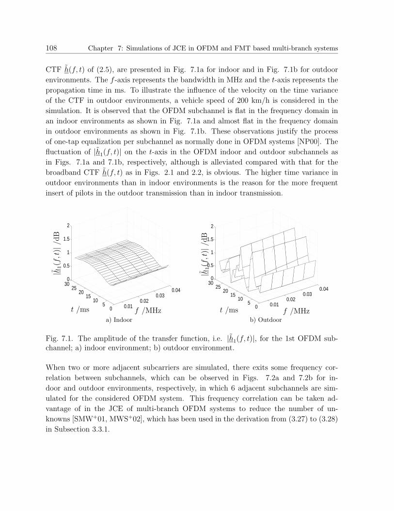
108 Chapter 7: Simulations of JCE in OFDM and FMT based multi-branch systems
CTF h(f, t) of (2.5), are presented in Fig. 7.1a for indoor and in Fig. 7.1b for outdoor
environments. The f -axis represents the bandwidth in MHz and the t-axis represents the
propagation time in ms. To illustrate the influence of the velocity on the time variance
of the CTF in outdoor environments, a vehicle speed of 200 km/h is considered in the
simulation. It is observed that the OFDM subchannel is flat in the frequency domain in
an indoor environments as shown in Fig. 7.1a and almost flat in the frequency domain
in outdoor environments as shown in Fig. 7.1b. These observations justify the process
of one-tap equalization per subchannel as normally done in OFDM systems [NP00]. The
fluctuation of |h1(f, t)| on the t-axis in the OFDM indoor and outdoor subchannels as
in Figs. 7.1a and 7.1b, respectively, although is alleviated compared with that for the
broadband CTF h(f, t) as in Figs. 2.1 and 2.2, is obvious. The higher time variance in
outdoor environments than in indoor environments is the reason for the more frequent
insert of pilots in the outdoor transmission than in indoor transmission.
0.010.02
0.030.04
05
1015
2025
300
0.5
1
1.5
2
f /MHzt /ms
|h1(f,t
)|/d
B
a) Indoor
0.010.02
0.030.04
05
1015
2025
300
0.5
1
1.5
2
f /MHzt /ms
|h1(f,t
)|/d
B
b) Outdoor
Fig. 7.1. The amplitude of the transfer function, i.e. |h1(f, t)|, for the 1st OFDM sub-channel; a) indoor environment; b) outdoor environment.
When two or more adjacent subcarriers are simulated, there exits some frequency cor-
relation between subchannels, which can be observed in Figs. 7.2a and 7.2b for in-
door and outdoor environments, respectively, in which 6 adjacent subchannels are sim-
ulated for the considered OFDM system. This frequency correlation can be taken ad-
vantage of in the JCE of multi-branch OFDM systems to reduce the number of un-
knowns [SMW+01, MWS+02], which has been used in the derivation from (3.27) to (3.28)
in Subsection 3.3.1.

7.3 Performance of JCE in the multi-branch OFDM system 109
00.05
0.10.15
0.20.25
05
1015
2025
300
0.5
1
1.5
2
2.5
f /MHzt /ms
|h1−
6(f,t
)|/d
B
a) Indoor
00.05
0.10.15
0.20.25
05
1015
2025
300
0.5
1
1.5
2
2.5
f /MHzt /ms
|h1−
6(f,t
)|/d
B
b) Outdoor
Fig. 7.2. The amplitude of the transfer function, i.e. |h1−6(f, t)|, for the 1st to the 6thOFDM subchannels; a) indoor environment; b) outdoor environment.
7.3.2 MSE simulation
The MSE in this subsection evaluates the performance of the FD-LS-JCE hLS of (3.34)
during the transmission of the pilot block with respect to the real channel during this
transmission period. Therefore, the real estimation performance is reflected and the
time variance of the channels from the transmission of the regarding pilot block to the
transmission of the following data blocks is not considered. The normalized MSE
ε′LS = εLS/U, (7.11)
which is obtained by dividing the MSE εLS of (3.50) by the number of branches U , is
presented in the simulation results. The optimum disjoint pilots, Walsh code based pilots
and CAZAC pilots constructed in Subsection 4.3.2, Subsection 4.3.3 and Subsection 4.3.4,
respectively, and the suboptimum random pilots discussed in Section 4.4 are used as the
pilots transmitted on the multiple branches in the simulations. A vehicle speed of 50
km/h is assumed and the channel is sufficiently estimated by FD-LS-JCE hLS of (3.34)
as explained in Subsection 7.2.1.
First, the indoor environments are considered. In Fig. 7.3 and Fig. 7.4, the normalized
MSEs ε′LS of (7.11) for the FD-LS-JCE hLS of (3.34) with Walsh code based pilots, disjoint
pilots, CAZAC code based pilots and random pilots are simulated under consideration of
1 MT and 1 AP, 2 MTs and 2 APs, 4 MTs and 4 APs as well as 8 MTs and 8 APs as
in Figs. 7.3a, 7.3b, 7.4a and 7.4b, respectively. The corresponding normalized minimum
MSE ε′LS,min of (3.59) is also shown in Figs. 7.3 and 7.4. It is seen that the normalized
MSE ε′LS of (7.11) of the FD-LS-JCE hLS of (3.34) with the optimum pilots like disjoint
pilots, Walsh code based pilots and CAZAC code based pilots always coincides with the

110 Chapter 7: Simulations of JCE in OFDM and FMT based multi-branch systems
normalized minimum MSE ε′LS,min of (3.59). For the FD-LS-JCE hLS of (3.34) using
random pilots, its MSE performance coincides with the normalized minimum MSE ε′LS,min
of (3.59) in the scenario of 1 MT and 1 AP of Fig. 7.3a. This is because in the case of
sufficient channel estimation, the MSE εLS obtained by applying FD-LS-JCE with any
pilots is calculated by 3.50. With one transmit branch, the random pilots statistically
produce the same value tr{((GHG)−1)} as the other pilots. However, in the multi-branch
cases of Figs. 7.3b, 7.4a and 7.4b, the higher the number of branches U , the worse
the MSE performance of FD-LS-JCE with random pilots compared to the normalized
minimum MSE ε′LS,min of (3.59). This is because the inter-branch interference is always
present for the FD-LS-JCE with random pilots. With large number of branches such as
with 8 MTs and 8 APs as in Fig. 7.4b, the MSE performance of FD-LS-JCE with random
pilots is extremely bad in comparison with the optimum pilots due to the inter-branch
interference. The simulation results in Figs. 7.3 and 7.4 demonstrate the necessity of the
investigation in this thesis on the design of optimum pilots for the multi-branch systems
especially with large number of branches.
0 5 10 15 20 25 3010
−5
10−4
10−3
10−2
10−1
100
101
102
103
Walsh code based pilotDisjoint pilotCAZAC code based pilotRandom pilotnormalized minimum MSE
normalized minimum MSE
SNR /dB
ε′ LS
a) 1 MT and 1 AP
0 5 10 15 20 25 3010
−5
10−4
10−3
10−2
10−1
100
101
102
103
Walsh code based pilotsDisjoint pilotsCAZAC code based pilotsRandom pilotsnormalized minimum MSE
normalized minimum MSE
SNR /dB
ε′ LS
b) 2 MTs and 2 APs
Fig. 7.3. The normalized MSE ε′LS of (7.11) and the normalized minimum MSE ε′LS,min of(3.59) for FD-LS-JCE with Walsh code based pilots, disjoint pilots, CAZAC code basedpilots and random pilots in the multi-user OFDM system in an indoor environment; a) 1MT and 1 AP; b) 2 MTs and 2 APs.

7.3 Performance of JCE in the multi-branch OFDM system 111
0 5 10 15 20 25 3010
−5
10−4
10−3
10−2
10−1
100
101
102
103
Walsh code based pilotsDisjoint pilotsCAZAC code based pilotsRandom pilotsnormalized minimum MSE
normalized minimum MSE
SNR /dB
ε′ LS
a) 4 MTs and 4 APs
0 5 10 15 20 25 3010
−5
10−4
10−3
10−2
10−1
100
101
102
103
Walsh code based pilotsDisjoint pilotsCAZAC code based pilotsRandom pilotsnormalized minimum MSE
normalized minimum MSE
SNR /dB
ε′ LS
b) 8 MTs and 8 APs
Fig. 7.4. The normalized MSE ε′LS of (7.11) and the normalized minimum MSE ε′LS,min of(3.59) for FD-LS-JCE with Walsh code based pilots, disjoint pilots, CAZAC code basedpilots and random pilots in the multi-user OFDM system in an indoor environment; a) 4MTs and 4 APs; b) 8 MTs and 8 APs.
Figs. 7.5a and Fig. 7.5b are obtained from some curves in Figs. 7.3 and 7.4 with emphasis
on the influence of the number of branches to the normalized MSEs ε′LS of (7.11) for FD-LS-
JCE hLS of (3.34) with optimum pilots, e.g. CAZAC code based pilots, and suboptimum
pilots, e.g. random pilots, in indoor environments. As seen in Fig. 7.5a, the number
of branches has no influence to the normalized MSEs ε′LS of (7.11) of FD-LS-JCE using
CAZAC code based pilots, which coincides always with the normalized minimum MSE
ε′LS,min of (3.59). This demonstrates that, with optimum pilots such as CAZAC code based
pilots, the MSE performance of FD-LS-JCE in multi-branch scenarios, e.g. 2 MTs and 2
APs, 4 MTs and 4 APs as well as 8 MTs and 8 APs, is the same with that in single-branch
scenario, e.g. 1 MT and 1 AP. This validates the theoretical expectation in Chapter 4, i.e.
the optimum pilots like CAZAC code based pilots should achieve the normalized minimum
MSE ε′LS,min of (3.59), which is independent of the number of branches U . However, as in
Fig. 7.5b, with random pilots, the inter-branch interference makes the MSE performance
of FD-LS-JCE worse in the multi-branch scenarios than in the single branch scenario.
The more the number of branches U , the worse the MSE performance for FD-LS-JCE
using random pilots.

112 Chapter 7: Simulations of JCE in OFDM and FMT based multi-branch systems
0 5 10 15 20 25 3010
−5
10−4
10−3
10−2
10−1
100
101
102
103
1MT, 1AP, JCE2MT, 2AP, JCE4MT, 4AP, JCE8MT, 8AP, JCEnormalized minimum MSE
normalized minimum MSE
SNR /dB
ε′ LS
a) CAZAC code based pilots
0 5 10 15 20 25 3010
−5
10−4
10−3
10−2
10−1
100
101
102
103
1MT, 1AP, JCE2MT, 2AP, JCE4MT, 4AP, JCE8MT, 8AP, JCEnormalized minimum MSE
normalized minumum MSE
SNR /dB
ε′ LS
b) Random pilots
Fig. 7.5. The normalized MSE ε′LS of (7.11) and the normalized minimum MSE ε′LS,min of(3.59) in the scenarios of 1MT-1AP, 2MT-2AP, 4MT-4AP and 8MT-8AP in multi-userOFDM system in an indoor environment; a) CAZAC code based pilots; b) random pilots.
In the following, the outdoor environments are considered. In Fig. 7.6 and Fig. 7.7, the
normalized MSEs ε′LS of (3.50) for the FD-LS-JCE hLS of (3.34) applying Walsh code
based pilots, disjoint pilots, CAZAC code based pilots and random pilots is simulated
under the scenarios of 1 MT and 1 AP, 2 MTs and 2 APs, 4 MTs and 4 APs as well as 8
MTs and 8 APs in Figs. 7.6a, 7.6b, 7.7a and 7.7b, respectively. The same tendency can
be seen as in indoor environments, i.e. the normalized MSEs ε′LS of (7.11) of FD-LS-JCE
with optimum pilots coincides with the normalized minimum MSE ε′LS,min of (3.59), while
the MSE performance of the FD-LS-JCE with random pilots gets worse when the number
of branches U increases.
0 5 10 15 20 25 3010
−5
10−4
10−3
10−2
10−1
100
101
102
103
Walsh code based pilotDisjoint pilotCAZAC code based pilotRandom pilotnormalized minimum MSE
normalized minimum MSE
SNR /dB
ε′ LS
a) 1 MT and 1 AP
0 5 10 15 20 25 3010
−5
10−4
10−3
10−2
10−1
100
101
102
103
Walsh code based pilotsDisjoint pilotsCAZAC code based pilotsRandom pilotsnormalized minimum MSE
normalized minimum MSE
SNR /dB
ε′ LS
b) 2 MTs and 2 APs
Fig. 7.6. The normalized MSE ε′LS of (7.11) and the normalized minimum MSE ε′LS,min of(3.59) for FD-LS-JCE with Walsh code based pilots, disjoint pilots, CAZAC code basedpilots and random pilots in the multi-user OFDM system in an outdoor environment; a)1 MT and 1 AP; b) 2 MTs and 2 APs.

7.3 Performance of JCE in the multi-branch OFDM system 113
0 5 10 15 20 25 3010
−5
10−4
10−3
10−2
10−1
100
101
102
103
Walsh code based pilotsDisjoint pilotsCAZAC code based pilotsRandom pilotsnormalized minimum MSE
normalized minimum MSE
SNR /dB
ε′ LS
a) 4 MTs and 4 APs
0 5 10 15 20 25 3010
−5
10−4
10−3
10−2
10−1
100
101
102
103
Walsh code based pilotsDisjoint pilotsCAZAC code based pilotsRandom pilotsnormalized minimum MSE
normalized minimum MSE
SNR /dB
ε′ LS
b) 8 MTs and 8 APs
Fig. 7.7. The normalized MSE ε′LS of (7.11) and the normalized minimum MSE ε′LS,min of(3.59) for FD-LS-JCE with Walsh code based pilots, disjoint pilots, CAZAC code basedpilots and random pilots in the multi-user OFDM system in an outdoor environment; a)4 MTs and 4 APs; b) 8 MTs and 8 APs.
In Fig. 7.8, the normalized MSEs ε′LS of (7.11) for FD-LS-JCE hLS of (3.34) using CAZAC
code based pilots and random pilots are illustrated with respect to the number of branches
U for outdoor environments. Similar to the simulation results in Fig. 7.5 for indoor
environments, in outdoor environments, the normalized MSEs ε′LS of (7.11) of FD-LS-JCE
with CAZAC code based pilots is independent on the number of considered branches U ,
while using random pilots it is sensitive to the number of branches U , as seen in Figs.
7.8a and 7.8b, respectively.
0 5 10 15 20 25 3010
−5
10−4
10−3
10−2
10−1
100
101
102
103
1MT, 1AP, JCE2MT, 2AP, JCE4MT, 4AP, JCE8MT, 8AP, JCEnormalized minimum MSE
normalized minimum MSE
SNR /dB
ε′ LS
a) CAZAC code based pilots
0 5 10 15 20 25 3010
−5
10−4
10−3
10−2
10−1
100
101
102
103
1MT, 1AP, JCE2MT, 2AP, JCE4MT, 4AP, JCE8MT, 8AP, JCEnormalized minimum MSE
normalized minimum MSE
SNR /dB
ε′ LS
b) Random pilots
Fig. 7.8. The normalized MSE ε′LS of (7.11) and the normalized minimum MSE ε′LS,min
of (3.59) in the scenarios of 1MT-1AP, 2MT-2AP, 4MT-4AP and 8MT-8AP in the multi-user OFDM system in an outdoor environment; a) CAZAC code based pilots; b) randompilots.

114 Chapter 7: Simulations of JCE in OFDM and FMT based multi-branch systems
To summarize this subsection, in the sufficient channel estimation case, as explained in
Subsection 7.2.1, the normalized MSE ε′LS of (7.11) for FD-LS-JCE hLS of (3.34) using
optimum pilots always coincides with the normalized minimum MSE ε′LS,min of (3.59).
The number of branches U has only influence to the normalized MSE ε′LS of (7.11) for
FD-LS-JCE hLS of (3.34) using suboptimum pilots like random pilots.
Although the MSE simulation results of only FD-LS-JCE are presented, it can be expected
that for the optimum pilots, e.g. disjoint pilots, Walsh code based pilots and CAZAC
code based pilots, there is no MSE performance difference between FD-MF-JCE and FD-
LS-JCE. This is because for optimum pilots, the matrix GHG in (3.34) is identity matrix
when the FD-LS-JCE hLS of (3.34) is compared with FD-MF-JCE hMF of (3.32). Besides,
for the multi-branch OFDM system, there is no MSE performance difference between FD-
LS-JCE and FD-WLS-JCE schemes. This is because for the OFDM modulation, the noise
before the channel estimator at the receiver is Gaussian [Fil04], i.e. the noise covariance
matrix is identity, when the FD-WLS-JCE hWLS of (3.37) is compared with FD-LS-JCE
hLS of (3.34).
7.3.3 BER simulation
The BER performance is obtained by comparing the detected data with the real trans-
mitted data during the transmission of data blocks. Since the channel information, which
is needed for equalization and/or reliable detection, is obtained by JCE before the trans-
mission of data blocks, the time variance of the subchannel, which is slow in indoor
environments according to the simulation result in Fig. 7.1a and fast in outdoor environ-
ments according to the simulation result in Fig. 7.1b, will influence adversely the BER
performance with FD-LS-JCE hLS of (3.34), even with the application of the optimum
pilots like Walsh code based pilots, disjoint pilots, and CAZAC code based pilots. In the
following JCE is called ideal JCE if the a-priori channel knowledge for data detection is
obtained as the real channel knowledge during the transmission of the data blocks. The
corresponding BER performance is illustrated in this subsection by the dotted curves.
Therefore, the BER curves with ideal JCE represent the best case without channel esti-
mation error due to the time variance of the channel during the data transmission period.
The vehicle speed of 50 km/h is taken in the simulations, and the channel is sufficiently
estimated by FD-LS-JCE as explained in Subsection 7.2.1 during the pilot transmission
period.
First, the indoor environments are considered. Figs. 7.9 and 7.10 illustrate the BER
performance when using Walsh code based pilots, disjoint pilots, CAZAC code based
pilots and random pilots for JCE in the cases of 1 MT and 1 AP, 2 MTs and 2 APs, 4
MTs and 4 APs as well as 8 MTs and 8 APs. It is seen in Fig. 7.9a that in the case of 1
MT and 1 AP, the BER performance when using the four kinds of pilots coincides with

7.3 Performance of JCE in the multi-branch OFDM system 115
each other, which is slightly worse than the ideal JCE case due to the slow time variance
of the channel in indoor environments. In the case of 2 MTs and 2 APs, as seen in Fig.
7.9b, the system with random pilots slightly underperforms that with the optimum pilots
of Walsh code based pilots, disjoint pilots and CAZAC code based pilots. By comparing
the curves in Fig. 7.9b with the curves in Figs. 7.10a and 7.10b, it is seen that the higher
the number of branches U , the worse the BER performance using random pilots than the
other optimum pilots. In general, the tendency of BER performance coincides with the
tendency of MSE performance as seen in Fig. 7.3 and Fig. 7.4. The higher the number
of branches U , the worse the BER performance of any optimum and suboptimum pilots
than the ideal JCE case due to the superposition of the signals on the multiple branches
at the receiver with the time variance of the channel on each branch.
SNR /dB
0 5 10 15 20 25 3010
−4
10−3
10−2
10−1
100
Walsh code based pilotDisjoint pilotCAZAC code based pilotRandom pilotperfect channel knowledge
BE
R
a) 1 MT and 1 AP
SNR /dB
0 5 10 15 20 25 3010
−4
10−3
10−2
10−1
100
Walsh code based pilotsDisjoint pilotsCAZAC code based pilotsRandom pilotsperfect channel knowledge
BE
R
b) 2 MTs and 2 APs
Fig. 7.9. The BER for Walsh code based pilots, disjoint pilots, CAZAC code based pilotsand random pilots in an indoor environment; a) 1 MT and 1 AP; b) 2 MTs and 2 APs.
SNR /dB
0 5 10 15 20 25 3010
−4
10−3
10−2
10−1
100
Walsh code based pilotsDisjoint pilotsCAZAC code based pilotsRandom pilotsperfect channel knowledge
BE
R
a) 4 MTs and 4 APs
SNR /dB
0 5 10 15 20 25 3010
−4
10−3
10−2
10−1
100
Walsh code based pilotsDisjoint pilotsCAZAC code based pilotsRandom pilotsperfect channel knowledge
BE
R
b) 8 MTs and 8 APs
Fig. 7.10. The BER for Walsh code based pilots, disjoint pilots, CAZAC code based pilotsand random pilots in an indoor environment; a) 4 MTs and 4 APs; b) 8 MTs and 8 APs.

116 Chapter 7: Simulations of JCE in OFDM and FMT based multi-branch systems
In Fig. 7.11, the BER performance under consideration of 1 MT and 1 AP, 2 MTs and 2
APs, 4 MTs and 4 APs, as well as 8 MTs and 8 APs in an indoor environment is compared
for CAZAC code based pilots, as illustrated in Fig. 7.11a, and for random pilots, as
illustrated in Fig. 7.11b. It is seen that in indoor environments, the BER performance for
the multi-branch OFDM system with CAZAC code based pilot transmission is slightly
sensitive to the number of branches U , while the BER performance with random pilot
transmission is very sensitive to the number of branches U . This is because with CAZAC
code based pilot transmission, the time variance of the indoor channel makes the estimated
channel of each branch by FD-LS-JCE hLS of (3.34) during the pilot transmission slightly
different from the real channel of each branch during the following data transmission.
While with random pilot transmission, not only the time variance of the indoor channel
during the pilot and data transmission influences adversely the BER performance, but also
the inter-branch interference in FD-LS-JCE hLS of (3.34) coming from the suboptimum
pilot transmission significantly deteriorates the BER performance. In the case of 8 MTs
and 8 APs, the BER performance with random pilot transmission is extremely bad. These
simulation results verify the necessity of the design of optimum pilots for FD-LS-JCE
especially in systems with large number of branches U .
SNR /dB
0 5 10 15 20 25 3010
−4
10−3
10−2
10−1
100
1MT, 1AP, practical JCE2MT, 2AP, practical JCE4MT, 4AP, practical JCE8MT, 8AP, practical JCEperfect channel knowledge
BE
R
a) CAZAC code based pilots
SNR /dB
0 5 10 15 20 25 3010
−4
10−3
10−2
10−1
100
1MT, 1AP, practical JCE2MT, 2AP, practical JCE4MT, 4AP, practical JCE8MT, 8AP, practical JCEperfect channel knowledge
BE
R
b) Random pilots
Fig. 7.11. The BER considering 1MT-1AP, 2MT-2AP, 4MT-4AP and 8MT-8AP in anindoor environment; a) CAZAC code based pilots; b) Random pilots.
Next, the BER performance in outdoor environments is presented. Figs. 7.12 and 7.13
show the BER curves when using Walsh code based pilots, disjoint pilots, CAZAC code
based pilots and random pilots and assuming 1 MT and 1 AP, 2 MTs and 2 APs, 4
MTs and 4 APs as well as 8 MTs and 8 APs. It is seen in Figs. 7.12a, 7.12b and 7.12a
that when considering a small number of branches U , there is little BER performance
difference between choosing optimum or suboptimum pilots for the pilot transmission.
That is because in both cases, the fast time variance of the outdoor channel during the
transmission of the pilot block and the following data blocks is more critical to the BER
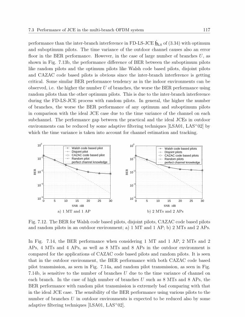
7.3 Performance of JCE in the multi-branch OFDM system 117
performance than the inter-branch interference in FD-LS-JCE hLS of (3.34) with optimum
and suboptimum pilots. The time variance of the outdoor channel causes also an error
floor in the BER performance. However, in the case of large number of branches U , as
shown in Fig. 7.13b, the performance difference of BER between the suboptimum pilots
like random pilots and the optimum pilots like Walsh code based pilots, disjoint pilots
and CAZAC code based pilots is obvious since the inter-branch interference is getting
critical. Some similar BER performance tendency as in the indoor environments can be
observed, i.e. the higher the number U of branches, the worse the BER performance using
random pilots than the other optimum pilots. This is due to the inter-branch interference
during the FD-LS-JCE process with random pilots. In general, the higher the number
of branches, the worse the BER performance of any optimum and suboptimum pilots
in comparison with the ideal JCE case due to the time variance of the channel on each
subchannel. The performance gap between the practical and the ideal JCEs in outdoor
environments can be reduced by some adaptive filtering techniques [LSA01, LAS+02] by
which the time variance is taken into account for channel estimation and tracking.
SNR /dB
0 5 10 15 20 25 3010
−4
10−3
10−2
10−1
100
Walsh code based pilotDisjoint pilotCAZAC code based pilotRandom pilotperfect channel knowledge
BE
R
a) 1 MT and 1 AP
SNR /dB
0 5 10 15 20 25 3010
−4
10−3
10−2
10−1
100
Walsh code based pilotsDisjoint pilotsCAZAC code based pilotsRandom pilotsperfect channel knowledge
BE
R
b) 2 MTs and 2 APs
Fig. 7.12. The BER for Walsh code based pilots, disjoint pilots, CAZAC code based pilotsand random pilots in an outdoor environment; a) 1 MT and 1 AP; b) 2 MTs and 2 APs.
In Fig. 7.14, the BER performance when considering 1 MT and 1 AP, 2 MTs and 2
APs, 4 MTs and 4 APs, as well as 8 MTs and 8 APs in the outdoor environment is
compared for the applications of CAZAC code based pilots and random pilots. It is seen
that in the outdoor environment, the BER performance with both CAZAC code based
pilot transmission, as seen in Fig. 7.14a, and random pilot transmission, as seen in Fig.
7.14b, is sensitive to the number of branches U due to the time variance of channel on
each branch. In the case of high number of branches U such as 8 MTs and 8 APs, the
BER performance with random pilot transmission is extremely bad comparing with that
in the ideal JCE case. The sensibility of the BER performance using various pilots to the
number of branches U in outdoor environments is expected to be reduced also by some
adaptive filtering techniques [LSA01, LAS+02].
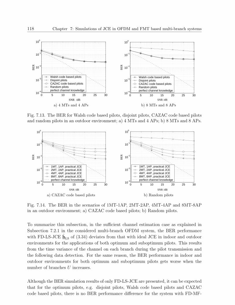
118 Chapter 7: Simulations of JCE in OFDM and FMT based multi-branch systems
SNR /dB
0 5 10 15 20 25 3010
−4
10−3
10−2
10−1
100
Walsh code based pilotsDisjoint pilotsCAZAC code based pilotsRandom pilotsperfect channel knowledge
BE
R
a) 4 MTs and 4 APs
0 5 10 15 20 25 3010
−4
10−3
10−2
10−1
100
Walsh code based pilotsDisjoint pilotsCAZAC code based pilotsRandom pilotsperfect channel knowledge
SNR /dB
BE
R
b) 8 MTs and 8 APs
Fig. 7.13. The BER for Walsh code based pilots, disjoint pilots, CAZAC code based pilotsand random pilots in an outdoor environment; a) 4 MTs and 4 APs; b) 8 MTs and 8 APs.
0 5 10 15 20 25 3010
−4
10−3
10−2
10−1
100
1MT, 1AP, practical JCE2MT, 2AP, practical JCE4MT, 4AP, practical JCE8MT, 8AP, practical JCEperfect channel knowledge
SNR /dB
BE
R
a) CAZAC code based pilots
0 5 10 15 20 25 3010
−4
10−3
10−2
10−1
100
1MT, 1AP, practical JCE2MT, 2AP, practical JCE4MT, 4AP, practical JCE8MT, 8AP, practical JCEperfect channel knowledge
SNR /dB
BE
R
b) Random pilots
Fig. 7.14. The BER in the scenarios of 1MT-1AP, 2MT-2AP, 4MT-4AP and 8MT-8APin an outdoor environment; a) CAZAC code based pilots; b) Random pilots.
To summarize this subsection, in the sufficient channel estimation case as explained in
Subsection 7.2.1 in the considered multi-branch OFDM system, the BER performance
with FD-LS-JCE hLS of (3.34) deviates from that with ideal JCE in indoor and outdoor
environments for the applications of both optimum and suboptimum pilots. This results
from the time variance of the channel on each branch during the pilot transmission and
the following data detection. For the same reason, the BER performance in indoor and
outdoor environments for both optimum and suboptimum pilots gets worse when the
number of branches U increases.
Although the BER simulation results of only FD-LS-JCE are presented, it can be expected
that for the optimum pilots, e.g. disjoint pilots, Walsh code based pilots and CAZAC
code based pilots, there is no BER performance difference for the system with FD-MF-
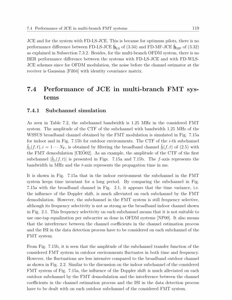
7.4 Performance of JCE in multi-branch FMT systems 119
JCE and for the system with FD-LS-JCE. This is because for optimum pilots, there is no
performance difference between FD-LS-JCE hLS of (3.34) and FD-MF-JCE hMF of (3.32)
as explained in Subsection 7.3.2. Besides, for the multi-branch OFDM system, there is no
BER performance difference between the systems with FD-LS-JCE and with FD-WLS-
JCE schemes since for OFDM modulation, the noise before the channel estimator at the
receiver is Gaussian [Fil04] with identity covariance matrix.
7.4 Performance of JCE in multi-branch FMT sys-
tems
7.4.1 Subchannel simulation
As seen in Table 7.2, the subchannel bandwidth is 1.25 MHz in the considered FMT
system. The amplitude of the CTF of the subchannel with bandwidth 1.25 MHz of the
WSSUS broadband channel obtained by the FMT modulation is simulated in Fig. 7.15a
for indoor and in Fig. 7.15b for outdoor environments. The CTF of the i-th subchannel
hi(f, t), i = 1 · · ·NF, is obtained by filtering the broadband channel h(f, t) of (2.5) with
the FMT demodulation [CEO02]. As an example, the amplitude of the CTF of the first
subchannel |h1(f, t)| is presented in Figs. 7.15a and 7.15b. The f -axis represents the
bandwidth in MHz and the t-axis represents the propagation time in ms.
It is shown in Fig. 7.15a that in the indoor environment the subchannel in the FMT
system keeps time invariant for a long period. By comparing the subchannel in Fig.
7.15a with the broadband channel in Fig. 2.1, it appears that the time variance, i.e.
the influence of the Doppler shift, is much alleviated on each subchannel by the FMT
demodulation. However, the subchannel in the FMT system is still frequency selective,
although its frequency selectivity is not as strong as the broadband indoor channel shown
in Fig. 2.1. This frequency selectivity on each subchannel means that it is not suitable to
use one-tap equalization per subcarrier as done in OFDM systems [NP00]. It also means
that the interference between the channel coefficients in the channel estimation process
and the ISI in the data detection process have to be considered on each subchannel of the
FMT system.
From Fig. 7.15b, it is seen that the amplitude of the subchannel transfer function of the
considered FMT system in outdoor environments fluctuates in both time and frequency.
However, the fluctuations are less intensive compared to the broadband outdoor channel
as shown in Fig. 2.2. Similar to the discussion on the indoor subchannel of the considered
FMT system of Fig. 7.15a, the influence of the Doppler shift is much alleviated on each
outdoor subchannel by the FMT demodulation and the interference between the channel
coefficients in the channel estimation process and the ISI in the data detection process
have to be dealt with on each outdoor subchannel of the considered FMT system.

120 Chapter 7: Simulations of JCE in OFDM and FMT based multi-branch systems
0 0.2 0.4 0.6 0.8 1 1.2 1.4
05
1015
2025
3035
0
0.5
1
1.5
2
t f /MHz
|h1(f,t
)|/d
B
a) Indoor
0 0.2 0.4 0.6 0.8 1 1.2 1.4
05
1015
2025
3035
−20
−15
−10
−5
0
5
t f /MHz
|h1(f,t
)|/d
B
b) Outdoor
Fig. 7.15. The amplitude of the transfer function, i.e. |h1(f, t)| for the 1st FMT subchan-nel; a) Indoor; b) Outdoor.
7.4.2 MSE simulation
In this subsection, the simulation results of the normalized MSE ε′LS of (7.11) for TD-LS-
JCE hLS of (3.86) over WSSUS channel in the multi-branch FMT systems are presented.
The optimum CAZAC code based pilots and the suboptimum random pilots are used as
the pilots transmitted on the multiple branches in the simulations.
In Fig. 7.16, the normalized MSE ε′LS of (7.11) for the multi-branch FMT system with
CAZAC code based pilots and random pilots in an indoor environment is simulated. Figs.
7.16a, 7.16b and 7.16c illustrate the cases with 1 MT and 1 AP, 2 MTs and 1 AP as well
as 3 MTs and 1 AP, respectively. It is seen that in the lower SNR range in the case of
1 MT and 1 AP, the MSE performance of TD-LS-JCE hLS of (3.86) with CAZAC code
based pilot is close to that with random pilot. Increasing the SNR, the MSE curve comes
to an error floor for TD-LS-JCE with random pilot transmission. While the error floor
has not appeared until the SNR of 25 dB for the MSE curve with CAZAC code based
pilot transmission. In the insufficient channel estimation, as explained in Subsection 7.2.2,
this error floor obtained by applying random pilot demonstrates that the TD-LS-JCE hLS
of (3.86) with random pilot is more sensitive than the CAZAC code based pilot to the
residue energy leakage by the mismatch between the number of channel coefficients W
and the number of channel taps, which is a random value. In the case of 2 MTs and 1 AP,
the TD-LS-JCE hLS of (3.86) with CAZAC code based pilots outperforms significantly
than that with random pilots in terms of the normalized MSE for the multi-branch FMT
system especially in the higher SNR range. This is because the inter-branch interference
in TD-LS-JCE using random pilots makes the error floor appear at low SNR value, while
there is no inter-branch interference in TD-LS-JCE using CAZAC code based pilots. In
the case of 3 MTs and 1 AP, the error floor can be observed for both CAZAC code
based pilot and random pilot transmissions. This is because the residue energy leakage of
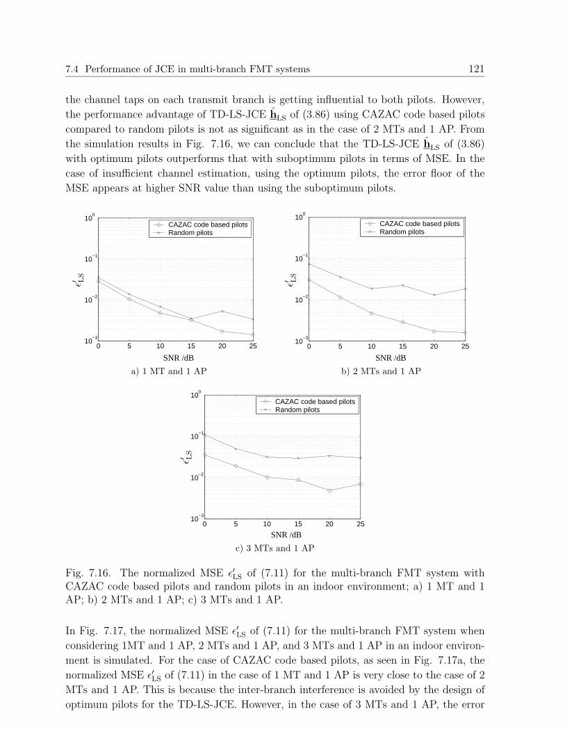
7.4 Performance of JCE in multi-branch FMT systems 121
the channel taps on each transmit branch is getting influential to both pilots. However,
the performance advantage of TD-LS-JCE hLS of (3.86) using CAZAC code based pilots
compared to random pilots is not as significant as in the case of 2 MTs and 1 AP. From
the simulation results in Fig. 7.16, we can conclude that the TD-LS-JCE hLS of (3.86)
with optimum pilots outperforms that with suboptimum pilots in terms of MSE. In the
case of insufficient channel estimation, using the optimum pilots, the error floor of the
MSE appears at higher SNR value than using the suboptimum pilots.
0 5 10 15 20 2510
−3
10−2
10−1
100
CAZAC code based pilotsRandom pilots
SNR /dB
ε′ LS
a) 1 MT and 1 AP
0 5 10 15 20 2510
−3
10−2
10−1
100
CAZAC code based pilotsRandom pilots
SNR /dB
ε′ LS
b) 2 MTs and 1 AP
0 5 10 15 20 2510
−3
10−2
10−1
100
CAZAC code based pilotsRandom pilots
SNR /dB
ε′ LS
c) 3 MTs and 1 AP
Fig. 7.16. The normalized MSE ε′LS of (7.11) for the multi-branch FMT system withCAZAC code based pilots and random pilots in an indoor environment; a) 1 MT and 1AP; b) 2 MTs and 1 AP; c) 3 MTs and 1 AP.
In Fig. 7.17, the normalized MSE ε′LS of (7.11) for the multi-branch FMT system when
considering 1MT and 1 AP, 2 MTs and 1 AP, and 3 MTs and 1 AP in an indoor environ-
ment is simulated. For the case of CAZAC code based pilots, as seen in Fig. 7.17a, the
normalized MSE ε′LS of (7.11) in the case of 1 MT and 1 AP is very close to the case of 2
MTs and 1 AP. This is because the inter-branch interference is avoided by the design of
optimum pilots for the TD-LS-JCE. However, in the case of 3 MTs and 1 AP, the error

122 Chapter 7: Simulations of JCE in OFDM and FMT based multi-branch systems
floor due to the insufficient channel estimation becomes significant so that the benefit of
TD-LS-JCE with CAZAC code based pilots in terms of the inter-branch interference free
estimation is not clearly seen. Nevertheless, when comparing Fig. 7.17a with Fig. 7.17b,
in which the random pilots are applied in the TD-LS-JCE for the multi-branch FMT
system, it is seen that with random pilots, the MSE performance of TD-LS-JCE suffers
not only from the error floor due to the insufficient channel estimation but also from the
inter-branch interference even in the case of low number of branches such as two transmit
branches.
0 5 10 15 20 2510
−3
10−2
10−1
100
1 MT and 1 AP2 MTs and 1 AP3 MTs and 1 AP
SNR /dB
ε′ LS
a) CAZAC code based pilots
0 5 10 15 20 2510
−3
10−2
10−1
100
1 MT and 1 AP2 MTs and 1 AP3 MTs and 1 AP
SNR /dB
ε′ LS
b) Random pilots
Fig. 7.17. The normalized MSE ε′LS of (7.11) for the multi-branch FMT system considering1 MT and 1 AP, 2 MTs and 1 AP, as well as 3 MTs and 1 AP in an indoor environment;a) CAZAC code based pilots; b) Random pilots.
In Fig. 7.18, the normalized MSE ε′LS of (7.11) for the multi-branch FMT system with
CAZAC code based pilots and random pilots in an outdoor environment is illustrated for
the cases of 1 MT and 1 AP, as shown in Fig. 7.18a, 2 MTs and 1 AP, as shown in Fig.
7.18b as well as 3 MTs and 1 AP, as shown in Fig. 7.18c. It is seen in Fig. 7.18a that
with only one transmit branch, the TD-LS-JCE hLS of (3.86) with CAZAC code based
pilot performs similar to that with random pilot transmission in terms of the normalized
MSE in the FMT system in lower SNR case. In higher SNR case, the TD-LS-JCE with
random pilot underperforms that with CAZAC code based pilot. The TD-LS-JCE with
both pilots suffers from more severe error floor in the MSE performance than in the indoor
environment as in Fig. 7.16. This is because in the outdoor environment, the maximum
channel delay is 5 µs, which is longer than 0.8 µs, which is assumed the maximum delay
in the indoor environment. In both environments, as mentioned in Subsection 7.2.2, the
number of channel coefficient W is set to 8, resulting in a more severe sensibility of TD-
LS-JCE for any pilots in the outdoor environment due to residue energy leakage of channel
taps. With two transmit branches, as seen in Fig. 7.18b, the TD-LS-JCE with CAZAC
code based pilots outperforms significantly than that with random pilots in terms of MSE
in the multi-branch FMT system. This is because the TD-LS-JCE with CAZAC code
based pilots has no inter-branch interference, while with random pilots has significant

7.4 Performance of JCE in multi-branch FMT systems 123
0 5 10 15 20 2510
−3
10−2
10−1
100
CAZAC code based pilotsRandom pilots
SNR /dB
ε′ LS
a) 1 MT and 1 AP
0 5 10 15 20 2510
−3
10−2
10−1
100
CAZAC code based pilotsRandom pilots
SNR /dB
ε′ LS
b) 2 MTs and 1 AP
0 5 10 15 20 2510
−3
10−2
10−1
100
CAZAC code based pilotsRandom pilots
SNR /dB
ε′ LS
c) 3 MTs and 1 AP
Fig. 7.18. The normalized MSE ε′LS of (7.11) for the multi-branch FMT system withCAZAC code based pilots and random pilots in an outdoor environment; a) 1 MT and 1AP; b) 2 MTs and 1 AP; c) 3 MTs and 1 AP.
inter-branch interference. With three transmit branches, as seen in Fig. 7.18c, the TD-
LS-JCE with CAZAC code based pilots performs also much better than that with random
pilots in terms of the normalized MSE in the multi-branch FMT system. However, the
advantage of CAZAC code based pilots over random pilots in the three branch case is not
as significantly as that in the two branch case due to the error floor in both cases which
comes from the insufficient channel estimation on each branch.
In Fig. 7.19, the normalized MSE ε′LS of (7.11) for the multi-branch FMT system con-
sidering 1 MT and 1 AP, 2 MTs and 1 AP, as well as 3 MTs and 1 AP in an outdoor
environment is illustrated. It is seen in Fig. 7.19a that with CAZAC code based pilots,
for the lower SNR range, the normalized MSE ε′LS of (7.11) in the 2 MTs and 1 AP case
is similar to that with 1 MT and 1 AP case. This verifies the theoretical analysis in
Chapter 4 that the normalized MSE performance for TD-LS-JCE with optimum pilots
like CAZAC code based pilots is not influenced by the number of branches U . However,

124 Chapter 7: Simulations of JCE in OFDM and FMT based multi-branch systems
in the higher SNR range and assuming a higher number U of branches such as three
branches, the MSE performance of CAZAC code based pilots is sensitive to the number
of branches due to the error floor that results from the insufficient channel estimation on
each branch. In comparison with the CAZAC code based pilots, with random pilots, as
shown in Fig. 7.19b, the MSE performance is very sensitive to the number of branches
with lower number of branches such as two branches. In the case of higher number of
branches such as three branches, the error floor of the MSE performance using random
pilot transmission appears at low SNR value due to the insufficient channel estimation on
each branch and the inter-branch interference. Therefore, it looks like the MSE perfor-
mance with random pilot transmission is not sensitive to the number of branches U when
U takes higher value.
0 5 10 15 20 2510
−3
10−2
10−1
100
1 MT and 1 AP2 MTs and 1 AP3 MTs and 1 AP
SNR /dB
ε′ LS
a) CAZAC code based pilots
0 5 10 15 20 2510
−3
10−2
10−1
100
1 MT and 1 AP2 MTs and 1 AP3 MTs and 1 AP
SNR /dB
ε′ LS
b) Random pilots
Fig. 7.19. The normalized MSE ε′LS of (7.11) of the multi-branch FMT system considering1 MT and 1 AP, 2 MTs and 1 AP, as well as 3 MTs and 1 AP in an outdoor environment;a) CAZAC code based pilots; b) Random pilots.
From above simulation results of MSE of the normalized MSE ε′LS of (7.11) of the estimated
channel in a multi-branch FMT system with various number of branches and with various
pilots, it is seen that in the scenario of insufficient channel estimation, the TD-LS-JCE hLS
of (3.86) with CAZAC code based pilot transmission outperforms that with random pilot
transmission in both indoor and outdoor environments. In addition, for the TD-LS-JCE
with CAZAC code based pilot transmission, the error floor appears at higher value than
that with random pilot transmission in both indoor and outdoor environments. This is
because although the MSE performance of TD-LS-JCE with both kinds of pilots suffers
from insufficient channel estimation, the TD-LS-JCE with random pilots deteriorates the
MSE performance further due to the inter-branch interference in channel estimation.
Although the MSE simulation results of only TD-LS-JCE are presented, it can be expected
that for the optimum pilots, e.g. CAZAC code based pilots, there is no MSE performance
difference for the system with TD-MF-JCE and for the system with TD-LS-JCE. This

7.4 Performance of JCE in multi-branch FMT systems 125
is because for optimum pilots, the matrix PHP in (3.86) is identity matrix when the
TD-LS-JCE hLS of (3.86) is compared with TD-MF-JCE hMF of (3.85). However, for the
multi-branch FMT system, there is MSE performance difference between TD-LS-JCE and
TD-WLS-JCE schemes [KWC04a]. This is because for the FMT modulation, the noise
before the channel estimator at the receiver is not Gaussian [KWC04a] after the FMT
demodulation at the receiver, i.e. the noise covariance matrix is not identity, when the
TD-WLS-JCE hWLS of (3.87) is compared with TD-LS-JCE hLS of (3.86).
7.4.3 BER simulation
In this subsection, the simulation results of the BER performance of the multi-branch
FMT system with TD-LS-JCE hLS of (3.86) are presented.
Fig. 7.20 shows the simulated BER curves for the multi-branch FMT system with CAZAC
code based pilots and random pilots in an indoor environment. In the case of 1 MT and
1 AP, as seen in Fig. 7.20a, the BER performance with CAZAC code based pilot trans-
mission is close to that with random pilot transmission. In the case of 2 MTs and 1 AP,
as seen in Fig. 7.20b, and in the case of 3 MTs and 1 AP, as seen in Fig. 7.20c, the
BER performance with CAZAC code based pilots applied to TD-LS-JCE outperforms
TD-LS-JCE with random pilots. Generally the inter-branch interference exists in both
the channel estimation and data detection stages. In Fig. 7.16, a significant MSE per-
formance advantage by using CAZAC code based pilots is seen than using random pilots
for the cases with two and three branches. This is because the inter-branch interference
in channel estimation is cancelled by TD-LS-JCE with CAZAC code based pilots. How-
ever, in the corresponding BER performance in Fig. 7.20, such significant advantage by
using CAZAC code based pilots over random pilots is not observed for the cases with two
and three branches. This is because the inter-branch interference in data detection ad-
versely significantly influences the BER performance using both CAZAC code based pilot
transmission and random pilot transmission. By introducing some advanced interference
suppressing and cancellation technologies in CDMA systems [Kle96], the inter-branch in-
terference in data detection will be mitigated, and the BER performance advantage by
using CAZAC code based pilot transmission over random pilot transmission is expected
to be significant.
In Fig. 7.21, the BER performance for the multi-branch FMT system considering 1 MT
and 1 AP, 2 MTs and 1 AP, and 3 MTs and 1 AP in an indoor environment is illustrated
for the application of CAZAC code based pilots, as shown in Fig. 7.21a, and for random
pilots, as shown in Fig. 7.21b. It is seen that with CAZAC code based pilots, the BER
performance for the multi-branch FMT system is not much sensitive to the number of
branches U . However, with random pilots, the BER performance is obviously worse in the
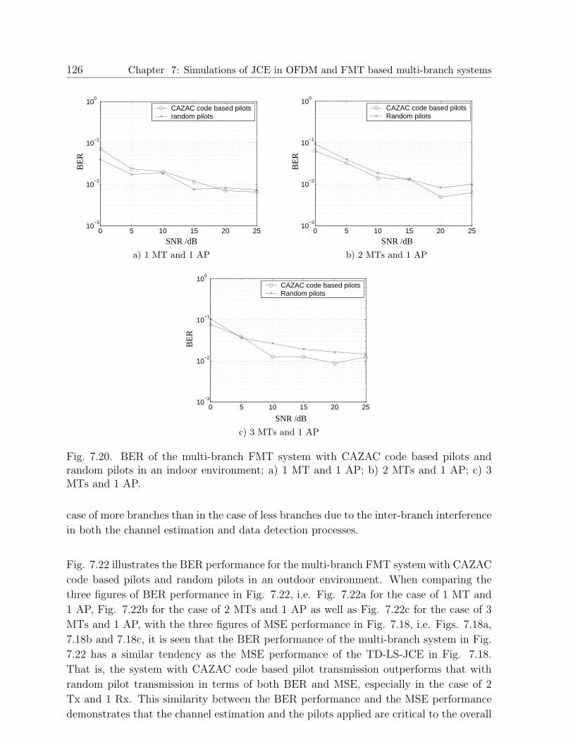
126 Chapter 7: Simulations of JCE in OFDM and FMT based multi-branch systems
0 5 10 15 20 2510
−3
10−2
10−1
100
CAZAC code based pilotsrandom pilots
SNR /dB
BE
R
a) 1 MT and 1 AP
0 5 10 15 20 2510
−3
10−2
10−1
100
CAZAC code based pilotsRandom pilots
SNR /dB
BE
R
b) 2 MTs and 1 AP
0 5 10 15 20 2510
−3
10−2
10−1
100
CAZAC code based pilotsRandom pilots
SNR /dB
BE
R
c) 3 MTs and 1 AP
Fig. 7.20. BER of the multi-branch FMT system with CAZAC code based pilots andrandom pilots in an indoor environment; a) 1 MT and 1 AP; b) 2 MTs and 1 AP; c) 3MTs and 1 AP.
case of more branches than in the case of less branches due to the inter-branch interference
in both the channel estimation and data detection processes.
Fig. 7.22 illustrates the BER performance for the multi-branch FMT system with CAZAC
code based pilots and random pilots in an outdoor environment. When comparing the
three figures of BER performance in Fig. 7.22, i.e. Fig. 7.22a for the case of 1 MT and
1 AP, Fig. 7.22b for the case of 2 MTs and 1 AP as well as Fig. 7.22c for the case of 3
MTs and 1 AP, with the three figures of MSE performance in Fig. 7.18, i.e. Figs. 7.18a,
7.18b and 7.18c, it is seen that the BER performance of the multi-branch system in Fig.
7.22 has a similar tendency as the MSE performance of the TD-LS-JCE in Fig. 7.18.
That is, the system with CAZAC code based pilot transmission outperforms that with
random pilot transmission in terms of both BER and MSE, especially in the case of 2
Tx and 1 Rx. This similarity between the BER performance and the MSE performance
demonstrates that the channel estimation and the pilots applied are critical to the overall

7.4 Performance of JCE in multi-branch FMT systems 127
0 5 10 15 20 2510
−3
10−2
10−1
100
1 MT and 1 AP2 MTs and 1 AP3 MTs and 1 AP
SNR /dB
BE
R
a) CAZAC code based pilots
0 5 10 15 20 2510
−3
10−2
10−1
100
1 MT and 1 AP2 MTs and 1 AP3 MTs and 1 AP
SNR /dB
BE
R
b) Random pilots
Fig. 7.21. BER of the multi-branch FMT system in the scenarios of 1 MT and 1 AP, 2MTs and 1 AP, as well as 3 MTs and 1 AP in an indoor environment; a) CAZAC codebased pilots; b) Random pilots.
system performance in the multi-branch FMT system.
In Fig. 7.23, the BER of the multi-branch FMT system considering 1 MT and 1 AP, 2
MTs and 1 AP, as well as 3 MTs and 1 AP in an outdoor environment is shown. When
the two subfigures in Fig. 7.23, i.e. Fig. 7.23a for CAZAC code based pilots and Fig.
7.23b for random pilots, are compared with the two figures in Fig. 7.19, i.e. Fig. 7.19a
and Fig. 7.19b, it is seen that the BER performance tendency for CAZAC code based
pilots and random pilots in the scenarios of various branches is the same as the MSE
performance tendency in the corresponding scenarios. This similarity also demonstrates
that the channel estimation and the pilots applied are influential to the overall system
performance in the multi-branch FMT system.
From above simulation results for the multi-branch FMT system of BER with various
number of branches and with various pilots, it is seen that in the scenario of insufficient
channel estimation, the BER performance has the similar tendency as the MSE perfor-
mance in both indoor and outdoor environments. Therefore, the investigations on the
channel estimation, especially on the pilot design in multi-branch systems, as carried out
in this thesis, is significant to the improvement of the overall system performance.

128 Chapter 7: Simulations of JCE in OFDM and FMT based multi-branch systems
0 5 10 15 20 2510
−2
10−1
100
CAZAC code based pilotsRandom pilots
SNR /dB
BE
R
a) 1 MT and 1 AP
0 5 10 15 20 2510
−2
10−1
100
CAZAC code based pilotsRandom pilots
SNR /dB
BE
R
b) 2 MTs and 1 AP
0 5 10 15 20 2510
−2
10−1
100
CAZAC code based pilotsRandom pilots
SNR /dB
BE
R
c) 3 MTs and 1 AP
Fig. 7.22. BER of the multi-branch FMT system with CAZAC code based pilots andrandom pilots in an outdoor environment; a) 1 MT and 1 AP; b) 2 MTs and 1 AP; c) 3MTs and 1 AP.

7.4 Performance of JCE in multi-branch FMT systems 129
0 5 10 15 20 2510
−2
10−1
100
1 MT and 1 AP2 MTs and 1 AP3 MTs and 1 AP
BE
R
SNR /dB
a) CAZAC code based pilots
0 5 10 15 20 2510
−2
10−1
100
1 MT and 1 AP2 MTs and 1 AP3 MTs and 1 AP
BE
R
SNR /dB
b) Random pilots
Fig. 7.23. BER of the multi-branch FMT system considering 1 MT and 1 AP, 2 MTsand 1 AP, as well as 3 MTs and 1 AP in an outdoor environment; a) CAZAC code basedpilots; b) Random pilots.

130 Chapter 8: Summary
8 Summary
8.1 English
Channel estimation is of great importance in many wireless communication systems, since
it influences the overall performance of a system significantly. Especially in multi-user
and/or multi-antenna systems, i.e. generally in multi-branch systems, the requirements
on channel estimation are very high, since the training signals or so called pilots that
are used for channel estimation suffer from multiple access interference. Recently, in
the context with such systems more and more attention is paid to concepts for joint
channel estimation (JCE) which have the capability to eliminate the multiple access in-
terference and also the interference between the channel coefficients. The performance
of JCE can be evaluated in noise limited systems by the SNR degradation and in in-
terference limited systems by the variation coefficient. Theoretical analysis carried out
in this thesis verifies that both performance criteria are closely related to the patterns
of the pilots used for JCE, no matter the signals are represented in the time domain or
in the frequency domain. Optimum pilots like disjoint pilots, Walsh code based pilots
or CAZAC code based pilots, whose constructions are described in this thesis, do not
show any SNR degradation when being applied to multi-branch systems. It is shown that
optimum pilots constructed in the time domain become optimum pilots in the frequency
domain after a discrete Fourier transformation. Correspondingly, optimum pilots in the
frequency domain become optimum pilots in the time domain after an inverse discrete
Fourier transformation. However, even for optimum pilots different variation coefficients
are obtained in interference limited systems. Furthermore, especially for OFDM-based
transmission schemes the peak-to-average power ratio (PAPR) of the transmit signal is
an important decision criteria for choosing the most suitable pilots. CAZAC code based
pilots are the only pilots among the regarded pilot constructions that result in a PAPR
of 0 dB for the transmit signal that origins in the transmitted pilots. When summariz-
ing the analysis regarding the SNR degradation, the variation coefficient and the PAPR
with respect to one single service area and considering the impact due to interference
from other adjacent service areas that occur due to a certain choice of the pilots, one can
conclude that CAZAC codes are the most suitable pilots for the application in JCE of
multi-carrier multi-branch systems, especially in the case if CAZAC codes that origin in
different mother codes are assigned to different adjacent service areas. The theoretical
results of the thesis are verified by simulation results. The choice of the parameters for
the frequency domain or time domain JCE is oriented towards the evaluated implementa-
tion complexity. According to the chosen parameterization of the regarded OFDM-based
and FMT-based systems it is shown that a frequency domain JCE is the best choice for
OFDM and a time domain JCE is the best choice for FMT applying CAZAC codes as
pilots. The results of this thesis can be used as a basis for further theoretical research
and also for future JCE implementation in wireless systems.

8.2 German 131
8.2 German
In zahlreichen drahtlosen Kommunikationssystemen kommt der Kanalschatzung eine große
Bedeutung zu, da sie die Gesamtperformanz eines Systems in erheblichem Maße beein-
flusst. Insbesondere in Mehrteilnehmersystemen und/oder Mehrantennensystemen, d.h.
allgemein in Systemen mit mehreren Ubertragungszweigen, werden hohe Anforderungen
an die Kanalschatzung gestellt, da die zur Kanalschatzung verwendeten Trainingssignale,
die sogenannten Piloten, Vielfachzugriffsinterferenzen unterliegen. Fur solche Systeme
werden zunehmend Verfahren zur gemeinsamen Kanalschatzung (engl. Joint Channel
Estimation, JCE) betrachtet, die sowohl die Vielfachzugriffsinterferenzen als auch die In-
terferenz zwischen den Kanal-Koeffizienten eliminieren. Die Performanz der JCE kann in
rauschbegrenzten Szenarien anhand der SNR-Degradation und in interferenzbegrenzten
Szenarien durch den Variationskoeffizienten evaluiert werden. Theoretische Analysen,
die in der vorliegenden Arbeit enthalten sind, zeigen, dass beide Performanzkriterien
eng mit der Struktur der zur Kanalschatzung verwendeten Piloten zusammenhangen,
unabhangig davon, ob die Piloten im Zeitbereich oder Frequenzbereich reprasentiert
werden. Optimale Piloten, wie beispielsweise nicht-gemeinsame Piloten, Walsh-Code-
basierende Piloten oder CAZAC-Code-basierende Piloten, deren Konstruktion in der
vorliegenden Arbeit beschrieben wird, weisen keine SNR-Degradation bei der Anwen-
dung in Systemen mit mehreren Ubertragungszweigen auf. Es wird gezeigt, dass opti-
male Piloten, die im Zeitbereich konstruiert werden, nach einer diskreten Fouriertrans-
formation zu optimalen Piloten im Frequenzbereich werden. Entsprechend werden opti-
male Piloten im Frequenzbereich durch eine inverse diskrete Fouriertransformation zu
optimalen Piloten im Zeitbereich. In interferenzbegrenzten Systemen zeigen sich je-
doch selbst fur optimale Piloten unterschiedliche Performanzen hinsichtlich des jeweili-
gen Variationskoeffizients. Insbesondere bei OFDM-basierten Ubertragungsverfahren ist
ein weiteres Kriterium zur Wahl geeigneter Piloten das durch das Senden der Pilotsig-
nale entstehende Verhaltnis zwischen maximalem Sendesignalpegel und mittlerem Sende-
signalpegel (engl. Peak-to-average power ratio, PAPR). CAZAC-Code-basierte Piloten
ermoglichen als einzige der hier betrachteten Piloten eine PAPR von 0 dB fur die fur die
Kanalschatzung erforderlichen Signalanteile. Fasst man die Analysen hinsichtlich SNR-
Degradation, Variationskoeffizienten und PAPR bezogen auf einen Versorgungsbereich
zusammen und betrachtet man die Auswirkungen auf die Interferenz, die zwischen un-
terschiedlichen Versorgungs-bereichen durch das Verwenden bestimmter Piloten erzeugt
wird, so lasst sich erkennen, dass CAZAC-Codes, die von unterschiedlichen Mutter-Codes
stammend unterschiedlichen Versorgungsbereichen zugeordnet werden, die am besten
geeigneten Piloten fur eine gemeinsame Kanalschatzung in einem Mehrtrager-Ubertra-
gungsverfahren mit mehreren Ubertragungszweigen sind. Die theoretischen Ergebnisse
dieser Arbeit sind durch Simulationen verifiziert. Die Wahl der Zeitbereichs-Kanalschat-
zung oder Frequenzbereichs-Kanalschat-zung richtet sich nach der Implementierungskom-
plexitat. Bei der gewahlten Parametrisierung der betrachteten OFDM-basierten und
FMT-basierten Systeme zeigt sich, dass fur OFDM eine Kanalschatzung im Frequenzbe-

132 Chapter 8: Summary
reich und fur FMT eine Kanalschatzung im Zeitbereich unter Verwendung von CAZAC-
Codes als Piloten die beste Wahl ist. Die vorliegende Arbeit kann sowohl als Basis fur
weiterfuhrende theoretische Analysen der gemeinsamen Kanalschatzung als auch als Basis
fur zukunftige Systemimplementierungen dienen.

A.1 Abbreviations 133
Appendix
A.1 Abbreviations
1G 1st Generation
2G 2nd Generation
3G 3rd Generation
4G 4th Generation
AP Acess Point
AWGN Additive White Gaussian Noise
BER Bit Error Rate
BS Base Station
CAZAC Constant Amplitude Zero Autocorrelation
cdf cumulative distribution function
CDMA Code Division Multiple Access
CIR Channel Impulse Response
CP Cyclic Prefix
CTF Channel Transfer Function
CU Central Unit
DFT Discrete Fourier Transformation
FB-MC Filter Bank Multi-Carrier
FD-JCE Frequency Domain Joint Channel Estimation
FD-MF-JCE Frequency Domain MF JCE
FD-LS-JCE Frequency Domain LS JCE
FD-WLS-JCE Frequency Domain Weighted LS JCE
FDMA Frequency Division Multiple Access
FFT Fast Fourier Transformation
FMT Filtered Multitone
IC Interference Cancellation
ICI Inter Carrier Interference
GSM Global System for Mobile Communications
IDFT Inverse Discrete Fourier Transformation
IFFT Inverse Fast Fourier Transformation
ISI Intersymbol Interference
JCE Joint Channel Estimation
JD Joint Detection
JOINT Joint Transmission and Detection Integrated Network
JT Joint Transmission
LOS Line-of-Sight
LS Least Square

134 Chapter 8: Summary
MAI Multiple Access Interference
MF Matched Filtering
MF-JCE Matched Filtering Joint Channel Estimation
MISO Multiple Input Single Output
ML Maximum Likelihood
MSE Mean Square Estimation Error
MMSE Minimum Mean Square Error
MT Mobile Terminal
NLOS No Line-of-Sight
OFDM Orthogonal Frequency Division Multiplexing
PAPR Peak to Average Power Ratio
pdf probability density function
PN Pseudo Noise
QoS Quality of Service
RF Radio Frequency
rrcos root raised cosine
SA Service Area
SISO Single Input Single Output
SS Spread Spectrum
SNR Signal–to–Noise Ratio
TD-CDMA Time Division CDMA
TDD Time Division Duplex
TD-JCE Time Domain JCE
TDMA Time Division Multiple Access
TD-MF-JCE Time Domain MF JCE
TD-LS-JCE Time Domain LS JCE
TD-WLS-JCE Time Domain Weighted LS JCE
TF Transfer Function
TD-SCDMA Time Division Synchronous CDMA
WCDMA Wideband CDMA
WLS Weighted Least Square
WSSUS Wide-Sense Stationary Uncorrelated Scattering
WSS Wide-Sense Stationary
A.2 Symbols
AC the matrix generated from the cyclic shifts of a CAZAC code
AW Hardamard matrix
B system bandwidth
BC channel coherence bandwidth
c speed of light
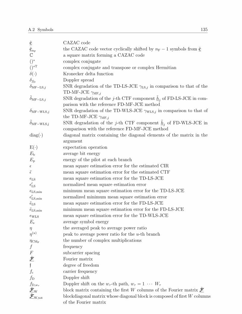
A.2 Symbols 135
c CAZAC code
cnFthe CAZAC code vector cyclically shifted by nF − 1 symbols from c
C a square matrix forming a CAZAC code
()∗ complex conjugate
()∗T complex conjugate and transpose or complex Hermitian
δ(·) Kronecker delta function
δfDDoppler spread
δMF−LS,j SNR degradation of the TD-LS-JCE γLS,j in comparison to that of the
TD-MF-JCE γMF,j
δMF−LS,j SNR degradation of the j-th CTF component hj of FD-LS-JCE in com-
parison with the reference FD-MF-JCE method
δMF−WLS,j SNR degradation of the TD-WLS-JCE γWLS,j in comparison to that of
the TD-MF-JCE γMF,j
δMF−WLS,j SNR degradation of the j-th CTF component hj of FD-WLS-JCE in
comparison with the reference FD-MF-JCE method
diag(·) diagonal matrix containing the diagonal elements of the matrix in the
argument
E(·) expectation operation
Eb average bit energy
Ep energy of the pilot at each branch
ε mean square estimation error for the estimated CIR
ε mean square estimation error for the estimated CTF
εLS mean square estimation error for the TD-LS-JCE
ε′LS normalized mean square estimation error
εLS,min minimum mean square estimation error for the TD-LS-JCE
ε′LS,min normalized minimum mean square estimation error
εLS mean square estimation error for the FD-LS-JCE
εLS,min minimum mean square estimation error for the FD-LS-JCE
εWLS mean square estimation error for the TD-WLS-JCE
Es average symbol energy
η the averaged peak to average power ratio
η(u) peak to average power ratio for the u-th branch
ηCMFthe number of complex multiplications
f frequency
F subcarrier spacing
F Fourier matrix
f degree of freedom
fc carrier frequency
fD Doppler shift
fD,wτDoppler shift on the wτ -th path, wτ = 1 · · · Wτ
FW block matrix containing the first W columns of the Fourier matrix F
FW,tot blockdiagonal matrix whose diagonal block is composed of firstW columns
of the Fourier matrix
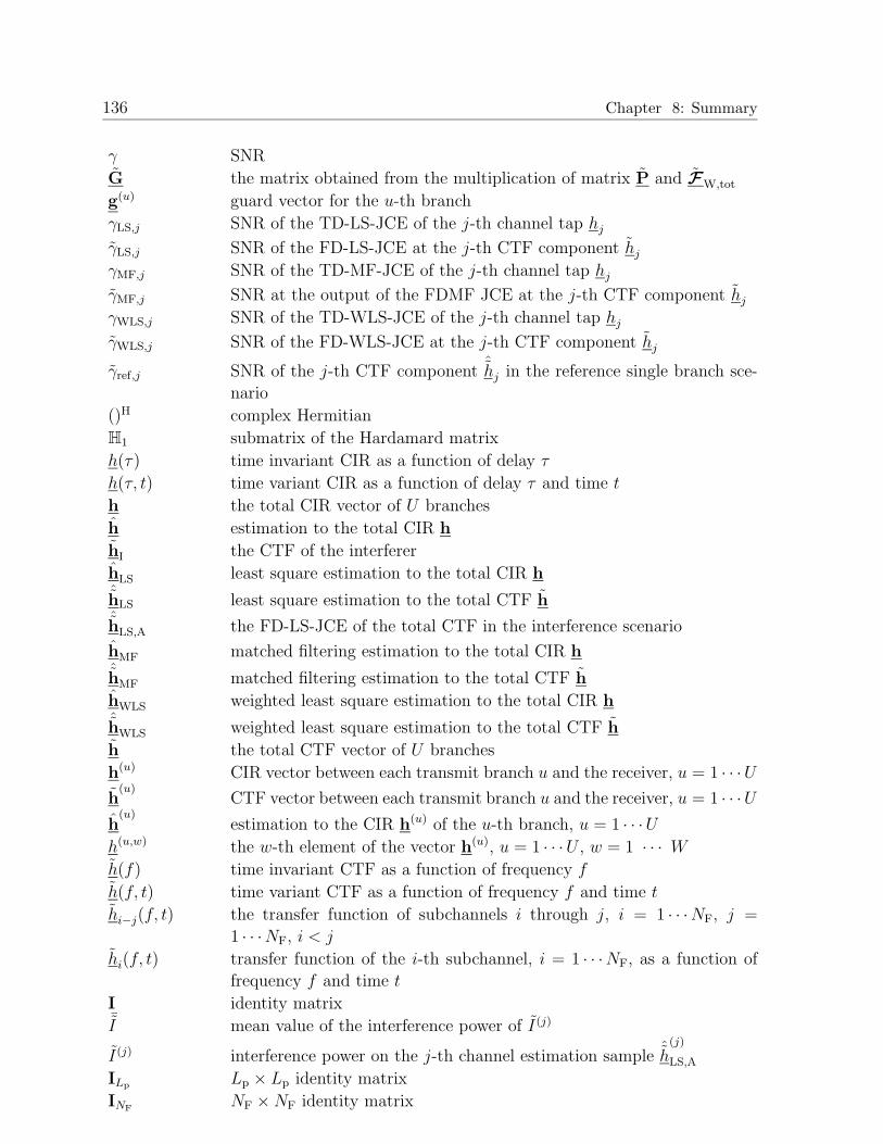
136 Chapter 8: Summary
γ SNR
G the matrix obtained from the multiplication of matrix P and FW,tot
g(u) guard vector for the u-th branch
γLS,j SNR of the TD-LS-JCE of the j-th channel tap hj
γLS,j SNR of the FD-LS-JCE at the j-th CTF component hj
γMF,j SNR of the TD-MF-JCE of the j-th channel tap hj
γMF,j SNR at the output of the FDMF JCE at the j-th CTF component hj
γWLS,j SNR of the TD-WLS-JCE of the j-th channel tap hj
γWLS,j SNR of the FD-WLS-JCE at the j-th CTF component hj
γref,j SNR of the j-th CTF component ˆhj in the reference single branch sce-
nario
()H complex Hermitian
H1 submatrix of the Hardamard matrix
h(τ) time invariant CIR as a function of delay τ
h(τ, t) time variant CIR as a function of delay τ and time t
h the total CIR vector of U branches
h estimation to the total CIR h
hI the CTF of the interferer
hLS least square estimation to the total CIR hˆhLS least square estimation to the total CTF hˆhLS,A the FD-LS-JCE of the total CTF in the interference scenario
hMF matched filtering estimation to the total CIR hˆhMF matched filtering estimation to the total CTF h
hWLS weighted least square estimation to the total CIR hˆhWLS weighted least square estimation to the total CTF h
h the total CTF vector of U branches
h(u) CIR vector between each transmit branch u and the receiver, u = 1 · · ·Uh
(u)CTF vector between each transmit branch u and the receiver, u = 1 · · ·U
h(u)
estimation to the CIR h(u) of the u-th branch, u = 1 · · ·Uh(u,w) the w-th element of the vector h(u), u = 1 · · ·U , w = 1 · · · Wh(f) time invariant CTF as a function of frequency f
h(f, t) time variant CTF as a function of frequency f and time t
hi−j(f, t) the transfer function of subchannels i through j, i = 1 · · ·NF, j =
1 · · ·NF, i < j
hi(f, t) transfer function of the i-th subchannel, i = 1 · · ·NF, as a function of
frequency f and time t
I identity matrix¯I mean value of the interference power of I(j)
I(j) interference power on the j-th channel estimation sample ˆh(j)
LS,A
ILp Lp × Lp identity matrix
INFNF ×NF identity matrix

A.2 Symbols 137
IUW identity matrix of dimension (UW ) × (UW )
IW identity matrix of dimension W ×W
J Lagrange cost function
K number of MTs simultaneously active in a cell or SA
ka number of antennas at each AP
KA number of APs
KM,k number of antennas at each MT k, k = 1 · · ·Kλj j-th eigenvalue of the matrix G
HG
LG guard interval length
Lp length of the pilot at each branch
M modulation order
M frequency domain estimation matrix
n time domain noise vector
n frequency domain noise vector
N0 one sided noise power spectral density
NF number of subcarriers
P a total time domain pilot matrix of U branches
P a total frequency domain pilot matrix of U branches
PC,w a NF × U submatrix containing U columns of the matrix AC
p(fD) pdf of the Doppler shift
p(fD, τ) joint pdf of the Doppler shift fD and the time delay τ
p(h) pdf of the CTF h(f, t)
p|h| pdf of the absolute value of the CTF h(f, t)
φh(τ, fD) the scattering function of the channel, which is obtained from the Fourier
transformation of φh(τ,∆t)
φh(τ1, τ2, t1, t2) autocorrelation function of the time-variant CIR h(τ, t) as a function of
τ1, τ2, t1, t2φ
h(τ,∆t) autocorrelation function of the time-variant CIR h(τ, t) as a function of
τ,∆t
φh(∆t,∆f) the time-frequency correlation function of the channel, which is ob-
tained from the Fourier transformation of the autocorrelation function
φh(∆t, τ)
φh(τ) power delay profile of the channel
P frequency domain total pilot matrix
p(u)
Ddisjoint pilot for the u-th branch
PI pilot matrix of the interferer
ψwτdirection of the terminal movement relative to the wτ -th path direction
p(fD) pdf of the Doppler shift fD
Pn average noise power
Ps average signal power
p(τ) pdf of the channel delay τ
p(τ, fD) joint pdf of the Doppler shift fD and time delay τ

138 Chapter 8: Summary
p(u) vector representing the time domain pilot transmit at each branch u, u =
1 · · ·Up(u)
Eextended pilot vector from the guard vector g(u) and the pilot vector
p(u) at the u-th branch
p(u) vector representing the frequency domain pilot transmit at each branch
u, u = 1 · · ·UP(u) a branch specific pilot matrix in time domain
P(u)
a diagonal branch specific pilot matrix in frequency domain
p(u,lp) the time domain pilot symbol value of the lp-th symbol at the u-th
branch, lp = 1 · · · Lp, u = 1 · · · Up(ϕ) pdf of the path phase
PW,w the w-th Walsh code based pilots
Q upsampling factor in filter bank multi-carrier systems
r the time domain receive signal vector
r the frequency domain receive signal vector
R correlation matrix of the total vector of CIR h
rA the interfered receive signal in the considered SA in the interference
scenario
Rb bit rate
rc cyclic correlation vector of the CAZAC code
R(i, j) the element in the correlation matrix R
Rh correlation matrix of the total CIR vector h
Rn covariance matrix of the time domain noise vector n
Rn covariance matrix of the frequency domain noise vector n
Rs symbol rate
σ2 power of the complex Gaussian noise vector
σ2h variation of the CTF h(t, f)
στ channel delay spread
σ2I mean square deviation of the interference power I(j)
smax maximum vehicle speed
t time
τ path delay in the radio channel
τmax maximum multi-path propagation delay
τwτpropagation delay of the wτ -th path, wτ = 1 · · · Wτ
T multi-carrier symbol duration
TC channel coherence time
TG guard interval duration
TOFDM total OFDM symbol duration
tr(·) trace operation
()T transpose of matrix
Ts symbol duration of the baseband signal
U number of branches

A.2 Symbols 139
v vehicle speed
V threshold level of the variation coefficients
vmax maximum vehicle speed
V unitary matrix
vc variation coefficient
ϕ random variable of the initial phase
ϕwτphase rotation of the wτ -th path, wτ = 1 · · · Wτ
W number of channel coefficients
wnFthe nF-th Walsh code obtained from the Hardamard matrix AW
Wτ number of channel taps
ZLS the estimation matrix in FD-LS-JCE
ZMF the estimation matrix in FD-MF-JCE
ZWLS the estimation matrix in FD-WLS-JCE
[·]x,y the element in the x-th row and the y-th column of a matrix in the
bracket
[·]x1,y1x2,y2
the submatrix bounded by the rows and and the columns and of a matrix
in the bracket

140 References
References
[Ala98] S.M. Alamouti, ”A Simple Transmit Diversity Technique for Wireless Com-munications”, IEEE Journal on Selective Areas in Communications, vol. 16,1998, pp. 1451–1458.
[Arf85] G. Arfken, Mathematical Methods for Physicists, Academic Press, 1985.
[BaM02] P.W. Baier, M. Meurer, ”Air interface enhancements for 3G and beyond-3G mobile radio communications”, Proc. 9th International Conference onTelecommunications (ICT ’02), 2002, pp. 284–291.
[BBT02] R. Berezdivin, R. Breinig, R. Topp, ”Next-generation wireless communica-tions concepts and technologies”, IEEE Communications Magazine, vol. 40,2002, pp. 108–116.
[BC02] N. Benvenuto, G. Cherubini, Algorithms for Communications Systems andTheir Applications, John Wiley & Sons, 2002.
[Bel63] P.A. Bello, ”Characterization of randomly time-variant linear channels”,IEEE Trans. Communication Systems, vol. CS-11, Dec. 1963, pp. 363–393.
[BES+95] J.v.d. Beek, O. Edfors, M. Sandell, S.K. Wilson, P.O. Borjesson, ”On chan-nel esimation in OFDM systems”,Proc. IEEE 45th Vehicular TechnologyConference, (VTC ’95), vol. 2, 1995, pp. 815–819.
[BJW01] P.W. Baier, C.A. Jotten, T. Weber, ”Review of TD-CDMA”, Proc. 3rd In-ternational Workshop on Commercial Radio Sencors and CommunicationsTechniques, (CRSCT ’01), 2001, pp. 11–20.
[BKN+94a] J.J. Blanz, A. Klein, M.M. Naßhan and A. Steil, “Capacity of a cellularCDMA mobile radio system applying joint detection”, COST 231 Tempo-rary Document TD (94) 2, Lisbon, 1994.
[BLM02] I. Barhumi, G. Leus, M. Moonen, ”Optimal trainging sequences for channelestimation in MIMO OFDM systems in mobile wireless channels”, Interna-tional Zurich Seminar on Broadband Communications, Access, Transmis-sion, Networking, 2002, pp. 44-1–44-6.
[Bol99] H. Bolcskei, ’Efficient design of pulse shaping filters for OFDM systems’,Proc. SPIE, vol. 3813, July 1999, pp. 625–636.
[BP95] K. Berberidis and J. Palicot, ”A frequency domain decision feedback equal-izer for multipath echo cancellation,”Proc. IEEE Global Telecommunica-tions Conference, (GLOBECOM ’95), vol. 1, 1995, pp. 98–102.
[BMW+00] P.W. Baier, M. Meurer, T. Weber, H. Troger, ”Joint Transmission (JT), analternative rationale for the downlink of time division CDMA using multi-element transmit antennas”, Proc. IEEE 6th International Symposium onSpread Spectrum Techniques & Applications, (ISSSTA ’00), vol. 1, 2000,pp. 1–5.
References 141
[BT02] N. Benvenuto, S. Tomasin, ”On the comparison between OFDM and singlecarrier modulation with a DFE using a frequency-domain feedforward filter”,IEEE Transactions on Communications, vol. 50, 2002, pp. 947–955.
[BTT02] N. Benvenuto, S. Tomasin, L. Tomba, ”Equalization methods in OFDM andFMT systems for broadband wireless communications”, IEEE Transactionson Communications, vol. 50, 2002, pp. 1413–1418.
[BTT02a] N. Benvenuto, S. Tomasin, L. Tomba, ”Receiver architectures for FMTbroadband wireless communications”, Proc. IEEE 53th Vehicular Technol-ogy Conference, (VTC ’01), vol. 1, 2001, pp. 643–647.
[CD02] Z. Cheng, D. Dahlhaus, ”Time versus frequency domain channel estima-tion for OFDM systems with antenna arrays”, Proc. IEEE 6th InternationalConference on Signal Processing, vol. 2, 2002, pp. 1340–1343.
[CEO02] G. Cherubini, E. Eleftheriou, S. Oker, ”Filtered multitone modulation forvery high-speed digital subscriber lines”, IEEE Journal on Selected Areasin Communications, vol. 20, 2002, pp. 1016–1028.
[CEO+00] G. Cherubini, E. Eleftheriou, S. Oker, J.M. Cioffi, ”Filter bank modulationtechniques for very high speed digital subscriber lines”, IEEE Communica-tions Magazine, vol. 38, 2000, pp. 98–104.
[CFW03] E. Costa, A. Filippi, M. Weckerle, E. Schulz, ”Comparision of FMT-FDMAand OFDMA in asynchronous uplink applications”, Proc. 8th InternationalOFDM Workshop (InOWo ’03), 2003.
[ChM00] W. Chen, U. Mitra, ”Frequency domain versus time domain based trainingsequence optimization”, Proc. IEEE International Conference on Commu-nications, (ICC ’00), vol. 2, 2000, pp. 646–650.
[Chu72] D.C. Chu, ”Polyphase codes with good periodic correlation properties”,IEEE Transactions on Information Theory, vol. 18, July 1972, pp. 531–532.
[ChM00a] W. Chen, U. Mitra, ”Training sequence optimization: comparisons and analternative criterion”, IEEE Transactions on Communications, vol. 48, Dec.2000, pp. 1987–1991.
[CM98] G. Caire, U. Mitra, ”Training sequence design for adaptive equalization ofmulti-user systems”, Proc. 32nd Asilomar Conference on Signals, Systems &Computers, vol. 2, 1998, pp. 1479–1483.
[COS89] COST 207, ”Digital land mobile radio communications”, Final ReportCOST Action 207, Office for Official Publications of the European Com-munities, Luxembourg, 1989.
[COS01] COST 259, ”Wireless flexible personalized communications”, Final ReportCOST Action 259, edited by L.M.Correia, John Wiley & Sons Inc., 2001.
[CS00] J. Chuang, N. Sollenberger, ”Beyond 3G: wideband wireless data accessbased on OFDM and dynamic packet assignment”, IEEE CommunicationsMagazine, vol. 38, 2000, pp. 78–87.
142 References
[CWG+01] M.V. Clark, T.M. Willis III, L.J. Greenstein, A.J. Rustako Jr., V. Erceg,R.S. Roman, ”Distributed versus centralized antenna arrays in broadbandwireless networks”, Proc. IEEE 53th Vehicular Technology Conference,(VTC ’01), vol. 1, 2001, pp. 33–37.
[DGE01] L. Deneire, B. Gyselinckx, M. Engels, ”Training sequences versus cyclic pre-fix – a new look on single carrier communication”, IEEE CommunicationsLetters, vol. 5, July 2001, pp. 292–294.
[DJ98] E.H. Dinan, B. Jabbari, ”Spreading codes for direct sequence CDMA andwideband CDMA celullar networks”, IEEE Communications Magazine,vol. 36, Sept. 1998, pp. 48–54.
[ECS+98] R.B. Ertel, P. Cardieri, K.W. Sowerbi, T.S. Rappaport and J.R. Reed,”Overview of spatial channel models for antenna array communication sys-tems”, IEEE Personal Communications Magazine, vol. 5, Feb. 1998, pp. 10–22.
[EGL93] M. Ewerbring, B. Gudmundson, G. Larsson, and P. Teder, ”CDMAwith interference cancellation: A technique for high capacity wireless sys-tems”, Proc. International Conference on Communications, May 1993,pp. 1901–1906.
[EMG99] V. Erceg, D.G. Michelson, S.S. Ghassemzadeh, L.J. Greenstein, et al., ”Amodel for the multipath delay profile of fixed wireless channels”, IEEE Jour-nal on Selected Areas in Communications, vol. 17, March 1999, pp. 399–410.
[FAB02] D. Falconer, S.L. Ariyavisitakul, A. Benyamin-Seeyar, B. Eidson, ”Fre-quency domain equalization for single-carrier broadband wireless systems”,IEEE Communications Magazine, vol. 40, April 2002, pp. 58–66.
[FAT03] C. Fragouli, N. Al-Dhahir, W. Turin, ”Training-based channel estimation formultiple-antenna broadband transmissions”, IEEE Transactions on WirelessCommunications, vol. 2, March 2003, pp. 384–391.
[FB92] T. Felhauer, P.W. Baier, ”Optimum radio channel estimation with periodicspread spectrum signal adjusted to amplifier nonlinearities”, Proc. IEEESecond International Symposium on Spread Spectrum Techniques and Ap-plications (ISSSTA ’92), 1992, pp. 309–312.
[Fel93] T. Felhauer, ”Digital signal processing for optimum wideband channel esti-mation in the presence of noise”, Proc. IEE F Radar and Signal Processing,vol. 140, June 1993, pp. 179–186.
[Fel94] T. Felhauer, Optimale erwartungstreue Algorithmen zur HochauflosendenKanalschatzung mit Bandspreizsignalformen, Fortschrittberichte VDI, series10, no. 278, VDI-Verlag, Dusseldorf, 1994.
[FG98] G.J. Foschini, M.J. Gans, ”On limits of wireless communications in a fadingenvironment when using multiple antennas”, Wireless Personal Communi-cations, vol. 6, 1998, pp.311–335.

References 143
[Fil04] A. Filippi, Non-conventional Multi-carrier Air Interface for the 4th Genera-tion Mobile Radio Systems, PhD thesis, 2004.
[Fis76] M. Fisz, Wahrscheinlichkeitsrechnung und Mathematische Statistik,Deutscher Verlag der Wissenschaften, Berlin, 1976.
[Fos96] G.J. Foschini, ”Layered space-time architecture for wireless communicationin a fading environment when using multi-element antennas”, Bell LabsTechnical Journal, Autumn 1996.
[FRB97] J. Fuhl, J.P. Rossi and E. Bonek, “High resolution 3-D direction-of-arrivaldetermination for urban mobile radio”, IEEE Transactions on Antennas andPropagation, vol. 45, 1997, pp. 672-681.
[FZH62] R.L. Frank, S.A. Zadoff, R. Heimiller, ”Phase shift pulse codes with goodperiodic correlation properties”, IRE Transactions on Information Theory,vol. 8, Oct. 1962, pp. 381–382.
[Gal01] D. Galda, ”The stochastic WSSUS broadband channel model and its impli-cations on the OFDM system design”, Technique Report of Joint Researchbeyond 3G (JRB3G) by Siemens, Aug. 2001.
[Gol67] R. Gold, ”Optimal binary sequences for spread spectrum multiplexing”,IEEE Transactions on Information Theroy, vol. 13, Oct. 1967, pp. 619–621.
[GSM88] ETSI/TC GSM Recommendations, series 01-12, 1988.
[Gar99] V.K. Garg, IS-95 CDMA & CDMA2000: Cellular/PCS Systems Implemen-tation, Prentice-Hall, 1999.
[Hei61] R.C. Heimiller, ”Phase shift pulse codes with good periodic correlation prop-erties”, IRE Transactions on Information Theroy, vol. 7, Oct. 1961, pp. 254–257.
[Hoe92] P. Hoeher, ”A statistical discrete-time model for the WSSUS multipathchannel”, IEEE Transactions on Vehicular Technology, vol. 41, Nov. 1992,pp. 461–468.
[HT02] H. Holma, A. Toskala, WCDMA for UMTS: Radio Access for Third Gen-eration Mobile Communications, John Wiley & Sons, 2002.
[Kal95] C.K. Kaleh, ”Channel equalization for block transmission systems”, IEEEJournal on Selected Areas in Communications, vol. 13, Jan. 1995, pp. 110–121.
[Kat97] R. Kattenbach, Charakterisierung zeitvarianter Indoor–Funkkanale anhandihrer System- und Korrelationsfunktionen, Shaker Verlag, Aachen, 1997.
[Kay93] S.M. KAY, Fundamentals of Statistical Signal Processing: Estimation the-ory, Ptentice-Hall, New Jersey, 1993.
144 References
[KCW+03] G. Kang, E. Costa, M. Weckerle, E. Schulz, ”Optimum channel estimationover frequency-selective fading channel in multiple antenna systems”, Proc.IEEE International Conference on Communication Technology, (ICCT ’03),vol. 2, 2003, pp. 1799–1803.
[KIH87] R. Kohno, H. Imai, M. Hatori, and S. Pasupathy, ”Adaptive cancellationof interference in direct-sequence spread-spectrum multiple access systems”,Proc. Global Telecommunications Conference, Nov. 1987, pp. 630–634.
[KJC+03] Y. Kim, B.J. Jeong, J. Chung, C. Hwang, J.S. Ryu, K. Kim, Y.K. Kim,”Beyond 3G: vision, requirements, and enabling technologies”, IEEE Com-munications Magazine, vol. 41, 2003, pp. 120–124.
[KKB96] A. Klein, K. Kaleh, P.W. Baier, ”Zero forcing and minimum-mean-square-error equalization for multiuser detection in code-division multiple-accesschannels”, IEEE Transactions on Vehicular Technology, vol. 45, May 1996,pp. 276–287.
[Kle96] A. Klein, Multi-user Detection of CDMA Signals – Algorithms and TheirApplications to Cellular Mobile Radio, VDI-Verlag GmbH, Dusseldorf, 1996.
[KMT96] A. Klein, W. Mohr, R. Thomas, P. Weber and B. Wirth, “Direction-of-arrival of partial waves in wideband mobile radio channels for intelligent an-tenna concepts”, Proc. IEEE 46th Vehicular Technology Conference (VTC’96), Atlanta, 1996, pp. 849–853.
[KMW+04] G. Kang, I. Maniatis, M. Weckerle, E. Costa, T. Weber, ”Optimum pilots forjoint channel estimation in multi-user OFDM systems”, IEEE Transactionson Wireless Communications, 2004, submitted.
[KWC04] G. Kang, M. Weckerle, E. Costa, ”Time and frequency domain joint channelestimation in multi-branch systems”, ICC ’04, submitted.
[KWC04a] G. Kang, M. Weckerle, E. Costa, ”Space-time joint channel estimation infiltered multi-tone based multi-carrier multi-branch systems”, Proc. IEEEWireless Communications and Networking Conference WCNC ’04, Atlanta,March 2004, pp. 1844-1849.
[Li00] Y. Li, ”Optimum training sequences for OFDM systems with multipletransmit antennas”,Proc. IEEE Global Telecommunications Conference,(GLOBECOM ’00), vol. 3, 2000, pp. 1478–1482.
[LL99] S. Li, J. Li, ”TD-SCDMA: standarlization and prototype development”,5th
Asia-Pacific Conference on Communications and 4th Optoelectronics andCommunications Conference, (APCC/OECC ’99) , vol. 2, 1999, pp. 1715.
[LSA99] Y. Li, N. Seshadri, S. Ariyavisitakul, ”Channel estimation for OFDM sys-tems with transmitter diversity in mobile wireless channels”, IEEE Journalon Selected Areas in Communications, vol. 17, 1999, pp. 461–471.
[LSA01] L. Lindbom, M. Sternad, A. Ahlen, ”Tracking of time-varying mobile ra-dio channels–part I: the Wiener LMS algorithm”, IEEE Transactions onCommunications, vol. 49, Dec. 2001, pp. 2207–2217.

References 145
[LAS+02] L. Lindbom, A. Ahlen, M. Sternad, M. Falkenstrom, ”Tracking of time-varying mobile radio channels–part II: a case study”, IEEE Transactionson Communications, vol. 50, Jan. 2002, pp. 156–167.
[MH97] S.H. Muller, J.B. Huber, ”OFDM with reduced peak-to-average power ratioby optimum combination of partial transmit sequences”, Electronics Letters,vol. 33, Feb. 1997, pp. 368–369.
[MWS+02] I. Maniatis, T. Weber, A. Sklavos, Y. Liu, E. Costa, H. Haas, E. Schulz, ”Pi-lots for joint channel estimation in multiuser OFDM mobile radio systems”,Proc. IEEE 7th International Symposium on Spread Spectrum Techniques& Applications, (ISSSTA ’02), vol. 1, 2002, pp. 44–48.
[NP00] R.V. Nee, R. Prasad, OFDM for Wireless Multimedia Communications,Artech House, 2000.
[Pap00] A. Papathanassiou, Adaptive antennas for mobile radio systems using TimeDivision CDMA and joint detection, Forschungsberichte Mobilkommunika-tion, vol. 6, University of Kaiserslautern, 2000, ISBN 3–925178–48–1.
[Par92] J.D. Parsons, The mobile radio propagation channel, Pentech Press, Lon-don, 1992.
[Pau94] A. Paulraj, et al., ”Increasing capacity in wireless broadcast system usingdistributed transmission/directional reception”, U.S. Patent no. 5345599,1994.
[PL95] K. Pahlavan and A.H. Levesque, Wireless Information Networks, New York:Wiley, 1995.
[Pro95] J.G. Proakis, Digital communications, McGraw–Hill, New York, 3rd edition,1995.
[Rap96] T.S. Rappaport, Wireless Communications principles and practice,Prentice-Hall, 1996.
[RGG01] H. Rohling, R. Grunheid, D. Galda, ”OFDM air interface for the 4-th gen-eration if mobile communication systems”, Proc. 6th International OFDM-workshop (InOWo ’01), Hamburg, Germany, Sept. 2001.
[Sch89] H. Schulze, ”Stochastische modelle und digitale simulation von mobil-funkkanalen”, in Kleinheubacher Berichte, no. 32, 1989.
[SG01] P. Struhsaker, K. Griffin, ”Analysis of PHY waveform peak to mean ratioand impact on RF amplification”, IEEE 802.16a cont. IEEE 802.16.3c-01/46,Mar. 6, 2001.
[SJ94] B. Steiner, P. Jung, ”Optimum and suboptimum channel estimation forthe uplink of CDMA mobile radio systems with joint detection”, EuropeanTransactions on Communications, vol. 5, 1994, pp. 39–49.
[Skl97] B. Sklar, ”Rayleigh fading channels in mobile digital communication sys-tems Part I: characterization”, IEEE Communications Magazine, Sept. 1997,pp. 136–146.

146 References
[SMH02] D. Schafhuber, G. Matz, F. Hlawatsch, ”Pulse-shaping OFDM/BFDM sys-tems for time-varying channels: ISI/ICI analysis, optimal pulse design, andefficient implementation”, Proc. IEEE 13th International Symposium on Per-sonal, Indoor and Mobile Radio Communications, (PIMRC ’02), vol. 3, 2002,pp. 1012–1016.
[SMW+01] A. Sklavos, I. Maniatis, T. Weber, P.W. Baier, E. Costa, H. Haas, E. Schulz,”Joint channel esitmation in multi-user OFDM systems”, Proc. 6th Interna-tional OFDM-workshop (InOWo ’01), 2001, pp. 3-1–3-4.
[SWB+01] A. Sklavos, T. Weber, P.W. Baier, E. Costa, ”Beyond 3G radio interfaceJOINT: optimum uplink data detection when applying OFDM”, Proc. 7th
International OFDM-workshop (InOWo ’02), 2002, pp. 11–15.
[Ste73] G.W. Stewart, Introduction to Matrix Computations, Academic Press, NewYork, 1973.
[SWB02] A. Sklavos, T. Weber, P.W. Baier, E. Costa, ”Beyond 3G radio interfaceJOINT: Optimum uplink data detection when applying OFDM”, Proc. 7th
International OFDM Workshop (InOWo ’02), 2002, pp. 11–15.
[Tel95] E. Telatar, ”Capacity of multi-antenna Gaussian channels”, AT&T Bell LabsInternal Techn. Memo., June 1995.
[TM97] F. Tufvesson, T. Maseng, ”Pilot assisted channel estimation for OFDM inmobile cellular systems”, Proc. IEEE 47th Vehicular Technology Conference,(VTC ’97), vol. 3, 1997, pp. 1639–1643.
[TSC98] V. Tarokh, N. Seshadri, A.R. Calderbank ”Space-time codes for high datarate wireless communication: performance criterion and code construction”,IEEE Trans. on Information Theory, vol. 44, 1998, pp. 744–765.
[Ver98] S. Verdu, Multiuser detection, Cambridge University Press, Cambridge,1998.
[VT01] F.W. Vook, T.A. Thomas, ”MMSE multi-user channel estimation for broad-band wireless communications”, Proc. Global Telecommunications Confer-ence (GLOBECOM ’01), 2001, pp. 470–474.
[Wec02] M. Weckerle, Utilization of Correlation Matrices in Adaptive Array Proces-sors for Time-slotted CDMA Uplinks, Kaiserslautern University, Disserta-tion, 2002.
[WeM02] T. Weber, M. Meurer, ”Iterative multiuser detection for TD-CDMA ex-ploiting data estimate refinement techniques”, Proc. IEEE 56th VehicularTechnology Conference, (VTC ’02 Fall), vol. 3, Sept. 2002, pp. 1642–1646.
[Wha71] A.D. Whalen, Detection of Signals in Noise, Academic Press, New York,1971.
[WCDMA] WCDMA specifications, ”Physical channels and mapping of transport chan-nels onto physical channels (FDD)”, 3GPP TS 25.211, v4.2.0, Sept. 2001.

References 147
[WMS+02] T. Weber, I. Maniatis, A. Sklavos, Y. Liu, E. Costa, H. Haas, E. Schulz,”Joint transmission and detection integrated network (JOINT), a genericproposal for beyond 3G systems”, Proc. 9th International Conference onTelecommunications, (ICT ’02), vol. 3, 2002, pp. 479–483.
[WNW01] D.A. Wiegandt, C.R. Nassar, Z. Wu, ”Overcoming peak-to-average powerratio issues in OFDM via carrier interferometry codes”, Proc. VehicularTechnology Conference, (VTC ’01), vol. 2, 2001, pp. 660–663.
[YMC02] K. Yang, A. Madhukumar, F. Chin, ”Optimum pilot design for multipathchannel estimation of a single carrier cyclic prefix-assisted CDMA system”,Proc. International Conference on Communication Systems, (ICCS ’02),vol. 1, 2002, pp. 279–283.
[Zol93] E. Zollinger, Eigenschaften von Funkubertragungsstrecken in Gebauden,Doctoral Dissertation, Eidgenossische Technische Hochschule Zurich, 1993.

148 Tabellarischer Lebenslauf
Tabellarischer Lebenslauf
Name: Guixia Kang
Birthday: 26. December 1972
Birth place: Tangshan, Heibei, China
Family status: Married
Nationality: Chinese
Education: Sept 1979 – July 1984Elementary School of Tianranqi Company, Daqing, Heilongjiang, China
Sept 1984 – July 1985Elementary School of the Second Extraction Factory, Daqing, China
Sept 1985 – July 1988The 30th Middle School of Daqing, Daqing, China
Sept 1988 – July 1991The Tieren High School of Daqing, Daqing, Heilongjiang, China
Study: Sept 1991 – July 1995Study of Industrial automationin Tianjin University
Graduation: Banchelor
Sept 1997 – Sept 2001Study of Wireless Communicationsin Beijing University of Posts and Telecommunications
Graduation: PhD
Work experience: August 1995 – August 1997Beijing Factory of Radio Instruments
Sept 1999 – July 2002Research scientist in Beijing University of Posts and Telecommunications
Since July 2002Free coworker of Siemens AG in Munich


![SGD Frequency-Domain Space-Frequency Semiblind Multiuser ... · Blind multiuser detection and channel estimation receivers based on subspace decomposition are proposed in [14-16]](https://img.pdfslide.us/doc/110x75/5fbcf1b8ce8bf14ede352c24/sgd-frequency-domain-space-frequency-semiblind-multiuser-blind-multiuser-detection.jpg)