Learning Time 1

Time and Associative Learning

Peter D. Balsam & Michael R. DrewBarnard College, Columbia University

C. R. GallistelRutgers University

In a basic associative learning paradigm, learning is said to have occurred when the conditioned stimulus evokes an antici-patory response. This learning is widely believed to depend on the contiguous presentation of conditioned and uncondi-tioned stimulus. However, what it means to be contiguous has not been rigorously defined. Here we examine the empirical bases for these beliefs and suggest an alternative view based on the hypothesis that learning about the temporal relationships between events determines the speed of emergence, vigor and form of conditioned behavior. This temporal learning oc-curs very rapidly and prior to the appearance of the anticipatory response. The temporal relations are learned even when no anticipatory response is evoked. The speed with which an anticipatory response emerges is proportional to the informative-ness of the predictive cue (CS) regarding the rate of occurrence of the predicted event (US). This analysis gives an account of what we mean by “temporal pairing” and is in accord with the data on speed of acquisition and basic findings in the cue competition literature. In this account, learning depends on perceiving and encoding temporal regularities rather than stimulus contiguities.

Keywords: Associative learning, conditioning, information theory, time

Time, contiguity and learning

In his essay On Memory and Reminiscence, Aristotle laid out principles specifying how the relationships between two events affected the ability of one event to act as a reminder of the second one. He posited that if events had been presented contiguously in time or space that one event would remind you of the other. The British empiricists posited that all knowledge was acquired through experience and used Aristotle’s memory retrieval principles as rules for the formation of the associations. During the 20th century

associationism became the foundation of psychology, and temporal contiguity emerged as the primary principle of learning. Theorists disagreed over what needed to be contiguous and what was learned (Guthrie, 1942; Hull, 1942; Pavlov, 1927; Skinner, 1961). Some focused on associations between stimuli; others focused on associations between stimuli and responses; others ignored associations (as unobservable); but they all agreed that whatever learning took place occurred because of contiguity.

In the 1960’s and 70’s, evidence began to accumulate that posed a challenge to the simple contiguity assumption. Cue competition phenomena [overshadowing (Kamin, 1969b); blocking (Kamin, 1969a); relative validity (Wagner, Logan, Haberlandt, & Price, 1968); and the truly random control (Rescorla, 1968)] demonstrated that repeated temporal contiguity between a potential cue (CS, for conditioned stimulus) and a motivationally important event (US, for unconditioned stimulus) did not necessarily lead to learning

This research was supported by by NIH (R01MH068073 to PDB, R01MH077027 to CRG and K99MH083943 to MRD) as well as support from NARSAD (to MRD). We thank R.Church, R. Miller, I. Nemenman, T. Ohyma, E. Shea-Brown and P. Dayan for comments on earlier versions of the manuscript.

Correspondence concerning this article should be addressed to Peter Balsam, Psychology Department, Barnard College, Columbia University, New York, NY 10027. E-mail: Balsam@ Columbia.edu

Volume 5, pp 1-222010

ISSN: 1911-4745 doi: 10.3819/ccbr.2010.50001 © Peter Balsam 2010

Learning Time 2

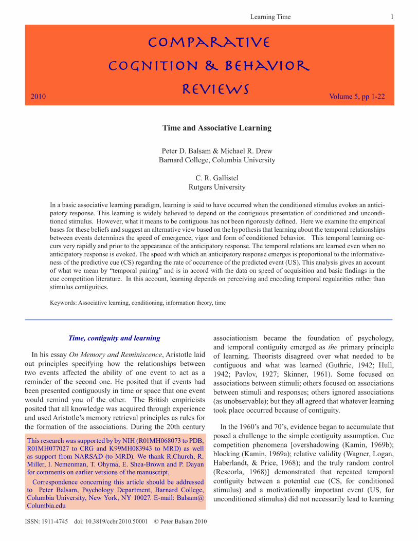
(Figure 1). It appeared that the key aspect of a protocol was not the temporal contiguity between the predictor (the CS) and the predicted (the US) but rather the information that the predictor provided about the predicted event (Rescorla, 1968). Within a few years, however, Rescorla and Wagner (1972) salvaged the associative framework by postulating that the amount of learning that occurred depended on the discrepancy between what the subject expected and the outcome on each trial. Thus, when there were multiple cues present during learning, the strength of conditioning to one cue limited the possible learning to other cues (cue competition). This reformulation had a several important consequences for the subsequent development of learning theory.

The strength of an association was now interpreted as the strength of an expectation. Also, associative strengths became mathematically processed quantities: The strengths of different associations could be summed, the sum could be subtracted from a hypothetical asymptote of expectation, and the resulting difference multiplied by yet another quantity (a learning rate) to determine how much a subject’s experience would change its expectation on a given trial. Cue competition effects no longer posed a problem for the assumption that temporal contiguity of cues triggered the recomputation of associative strength. Events were considered contiguous if they occurred on the same trial, but it was acknowledged that the problem of precisely defining what constituted contiguity remained unresolved (Gluck & Thompson, 1987; Rescorla, 1988; Rescorla & Wagner, 1972). This version of contiguity theory now guides work on the neurobiology of learning. It proceeds on the assumptions that the changes that underlie

learning are pairing-dependent (Fanselow & Poulos, 2005; Hawkins, Kandel, & Bailey, 2006; Thompson, 2005) and that they occur only when events are unexpected (Schultz, 2006; Schultz, Dayan, & Montague, 1997).

Contiguity and Learning

Contiguity is so embedded in our beliefs about what is necessary for learning that it is worth examining the experimental evidence that underlies this hypothesis. Our empirical belief in contiguity comes from studies that vary the time from the onset of the CS till the presentation of the US. When this CS-US interval is lengthened, a decrement in conditioning is observed (it takes more trials for the conditioned response (CR) to appear, and CR strength is often reduced). If the CS remains on until the US occurs, the procedure is called delay conditioning. If there is a gap between CS offset and the US, the procedure is known as trace conditioning.

The detrimental effect of increasing the CS-US interval on the amount of conditioned responding has been observed in a wide range of preparations including autoshaping (Gibbon, Baldock, Locurto, Gold, & Terrace, 1977), eyeblink (Gormezano & Kehoe, 1981; Reynolds, 1945; Smith, 1968), paw flexion (Wickens, Meyer, & Sullivan, 1961), salivary (Ost & Lauer, 1965) and heart rate (Vandercar & Schneiderman, 1967) conditioning as well as in the conditioned emotional response paradigm (Stein, Sidman, & Brady, 1958).

These findings appear to support a contiguity theory of learning. However, the effect of a given delay to

USCSContingent λ

CS> λ

C

Truly Random λ

CS= λ

C

t

t

ITIT

λCS

=2/(3T)

λCS

=2/(3T)

λC=2/t

λC=11/t

0

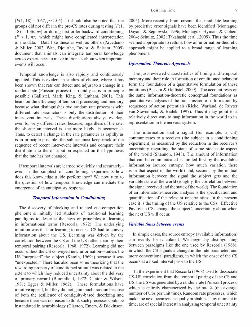
0Figure 1. Schematic of the experimental protocols by which (Rescorla, 1968) demonstrated that CS-US contingency, not the temporal pairing of the CS and US, produces a US-anticipatory response (CR). The temporal pairing of CS and US is identical in the two groups, but there is no CS-US contingency in the second group (the truly random control), because the US occurs as frequently in the absence of the CS as in its presence, that is, lCS = lC. The subjects in the Group 1 develop a conditioned response to the CS; the subjects in Group 2 do not. (They did, however, develop a conditioned response to the context, that is, to the experimental chamber.) This was one of the findings that called into question the foundational assump-tion that the learning mechanism was activated by the temporal pairing of CS and US. CS=the conditioned stimulus (e.g., a tone); US = the unconditioned stimulus (e.g., shock to the feet); ITI=intertrial interval; T=duration of a CS presentation.

Learning Time 3

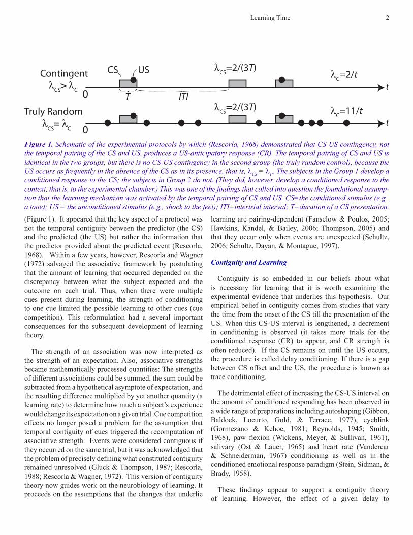
reinforcement depends on the intertrial interval. Figure 2 shows the effect of varying the CS-US interval on the speed of acquisition in a form of Pavlovian delay conditioning known as autoshaping (Gallistel & Gibbon, 2000). The red line comes from experimental groups in which the interval between trials (ITI) was fixed at 48s. As expected, the greater the delay to reinforcement (T), the more pairings it takes before responding emerges. The groups represented by the blue line had identical delays to reinforcement. However, in these groups the interval between the trials was increased in proportion to the increase in the duration of the delay. For example, when the CS duration was increased from 4 to 8 s the ITI was doubled from 48 to 96 s. The remarkable finding is that so long as the relative proximity to reward is maintained, acquisition speed is approximately constant. This has been a rich source of theorizing about Pavlovian conditioning (Balsam, Sanchez-Castillo, Taylor, Van Volkinburg, & Ward, 2009; Gallistel & Gibbon, 2000; Gibbon & Balsam, 1981).

In an attempt to save contiguity as the basic learning principle Gibbon & Balsam (1981) posited that performance was a function of the ratio of the associative value of cues to the background values. That is, the excitatory strength of a cue depended not on any absolute value but on the cue value relative to a context. In this view, the intervals between reinforcements set the asymptote of associative value for the context (that is, the background rate of reinforcement) and the delay from the onset of a cue until reinforcement set the asymptote for the cue. Thus contiguity could still underlie the independent learning of cue and context values. However, there is a paradox in this relativised contiguity view. It asserts that the temporal relationship between events is learned extremely rapidly in order to set asymptotes but then this non-associative learning of a critical temporal parameter is followed by a slower associative learning process. It is not clear then what learning if any depends on contiguity.

The effect of the second way of varying contiguity on responding to a CS is shown in the left side of Figure 3.

Med

ian

Rein

forc

emen

tsto

Acq

uisi

tion

T (trial duration, in s)

ITI fixedITI/T fixed

0

160

140

120

100

80

60

40

20

0 3530252015105

Figure 2. Acquisition speed as a function of the duration of the trial CS. Pigeons were exposed to keylight CSs paired with food, at fixed delays that ranged from 4 s to 32 s. For some groups (red line), the intertrial interval (ITI) was fixed at 48s. As the delay (T) from CS onset to US presentation increased, the number of pairings before the appearance of the CR increased. For other groups (blue line), the ITI was increased in proportion to T. In these groups, trials to acquisition was constant. (Data from Gibbon et al., 1977.)

Learning Time 4

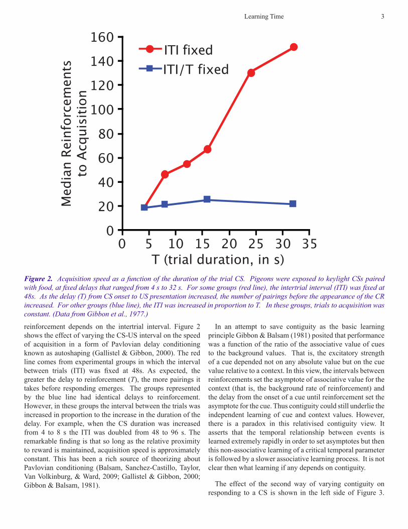
In this experiment two groups of rats were exposed to a 6 s tone CS, which was followed by pellet delivery after different trace intervals in two groups of subjects. (The interval between the offset of the CS and the onset of the US is called the trace interval because it has long been assumed that the residual sensory activity from the CS—its trace in the nervous system—slowly decays during this interval.) The CS was followed by a 6 sec trace interval in one group and an 18 s trace interval in the other group.

The bar graph on the left side of the figure shows that average CR strength during the CS was considerably lower in the subjects exposed to the longer trace interval. The right side of the graph shows the average response rate during the entire CS-US interval in both groups. The longer delay engenders a lower response rate but in both groups the subjects appear to know when to expect the food delivery. The lower level of responding would appear to reflect an accurate knowledge of when the reinforcer will be delivered (Brown, Hemmes, & Cabeza de Vaca, 1997). The knowledge that animals acquire about the temporal structure of events is quite rich: not only do they learn the interval from one US to the next and the interval from the onset of the CS until the US (Kirkpatrick & Church, 2000a), they also encode the interval from the offset of the CS until the US (Kehoe & Napier, 1991; Odling-Smee, 1978).

Another challenge to a simple contiguity account of learning is that temporal anticipation can occur over very long delays (Balsam et al., 2009). In a fixed interval schedule of reinforcement, the first response after some minimum

amount of time since the onset of a trial is reinforced. In some experiments, the delay until the next opportunity begins with the latest reinforcement; in others the beginning of the delay interval is signaled by a discrete cue. On these schedules, subjects show that they have learned the length of the delay by increasing their probability of responding as the expected time of reward approaches. There are studies that show accurate learning of these delays over several orders of magnitude: indeed, anticipation of food every fifty minutes is as accurate as anticipation of food every thirty seconds (Dews, 1970). Eckerman (1999) showed that when food was available once every 24 hours subjects began responding about an hour in advance. This high level of accuracy was probably the result of a circadian timing mechanism. However, when long but non-circadian (18-23 hr) fixed interval schedules were employed, subjects began responding several hours in advance. Similarly, Crystal has shown that animals use interval timers well into the hours range (Babb & Crystal, 2006; Crystal, 2006).

Animals are even sensitive to the passage of intervals that are measured in days. In a very clever set of experiments (Clayton, Yu, & Dickinson, 2001) trained jays to cache 3 different kinds of food: peanuts, wax worms and crickets. When tested 4 hours after burying their food, the birds preferred meal worms over crickets and peanuts. However, once the jays learned that worms decayed after 28 hours and crickets decayed after 100 hours, their preferences were guided by that knowledge in delayed retrieval tests. When tested 28 hours after caching, the birds retrieved crickets first, but when tested 100 hours after making their caches,

0

0.1

0.2

0.3

0.4

0.5

Group6-6 6-18

Entr

ies/

s

Entr

ies/

s

00 4 8 12 16 20 24

0.2

0.4

0.6

0.8

Time after CS Onset (s)Figure 3. The effects of fixing the CS duration and varying the trace interval from the offset of the CS until the US is pre-sented. Rats were exposed to a 6-s tone paired with food, with a 6- or 18-s trace interval. Anticipatory head entries into the feeding hopper were recorded. Left: The longer the trace interval, the less the average response rate during the CS. Right: Rate of responding as a function the CS-US interval. The break in the plots occurs at CS offset. Note the steady, appropriately-timed increase during the gap between CS offset and US onset.

Learning Time 5

the jays went for the peanuts. They knew the intervals since they had made their caches and the intervals required for different foods to rot. All these examples illustrate that animals are capable of learning about the relation between cues and outcomes over many hours and days, thus forcing us to consider whether there is utility in assuming that learning depends on contiguity.

There is yet another very troubling set of data that makes us wonder if the experiments we have taken as evidence for contiguity should be trusted at all. From a contiguity point of view, if one were to move the CS back in time from the US, eventually no learning would be expected to occur. However, whether or not we see the learning may depend on what is measured. When a CS is relatively proximal to a US, we expect to see anticipatory behavior. If the CS is remote enough from the US, there will be no anticipation, but that does not mean there was no learning. Kaplan (1984) did several experiments showing that when subjects are exposed to delays from CS to US that are long in relation to the expected interval between feedings, they do not show anticipatory behavior but instead show behavior that is appropriate for a signal that indicates a long wait for food: They withdraw from rather than approach the signal for food. This suggests that they learn the interval regardless of its length and that the behavioral manifestation of this learning depends on the length of the interval relative to the expected interval between reinforcing events.

More generally, cues that signal different temporal distances to outcomes may control qualitatively different responses. Holland (1980) exposed groups of rats to CSs of different durations paired with a food US. He found that the duration of the CS modulated the form of the CR. When auditory CSs were brief, they tended to evoke head-jerk CRs; when they were long, they evoked less head-jerking but much more magazine approach. Timberlake (2001) has suggested that motivational modes change with proximity to reinforcement. As food becomes more imminent, the subject switches from a general search mode to a focal search to a handling/consummatory mode. Each of these states will motivate different sets of behaviors. For example, general exploration of the environment will occur when animals are remote from food. As food becomes more proximal, attention to signals for food and prey stimuli will increase and, finally, food directed behavior will occur in anticipation of the reward. This change in response form as a function of proximity to reinforcement has been well documented (Domjan, 2003; Silva & Timberlake, 1997; Silva & Timberlake, 1998; Silva & Timberlake, 2005). Response topographies are determined by the relative —not absolute— proximity to reinforcement. Silva and Timberlake (1998) found that general search and focal search occurred at the same relative portion of the

interval as the absolute time between food was varied. Thus, relative proximity to reinforcement seems to also determine what response occurs. Consequently, experiments showing that increasing the time from the onset of a cue until the US reduces learning should be interpreted with great caution. The work cited above makes it seem likely that contiguity manipulations change the response evoked by the cue rather than interfere with underlying learning. Failures to observe anticipatory CRs should not be interpreted as failures of learning.

Learning Time

For all of the above reasons, we have become skeptical of the view that contiguity is the basic principle of learning, and we have offered an alternative view (Balsam & Gallistel, 2009): If animals rapidly learn the intervals between events, perhaps that is the foundation of the learning. The intervals between events are no longer simply the aspect of experience that conditions the formation of associations; rather the durations of those intervals and the proportions between them are the content or substance of learning itself. The strong version of this view is that temporal relationships between events are constantly and automatically encoded. These temporal relationships may be extracted even from single experiences. Further, the learning of the temporal intervals does not depend on the contiguity between events. What we have previously called associative learning is the emergence of anticipatory behavior founded on knowledge of these intervals. Because we have historically used anticipatory behavior as our index of learning we have been misled into equating learning and anticipation. They are not the same.

Learning Temporal Intervals

Learning time during conditioning: It has been recognized since the time of Pavlov CRs are timed. The emergence of a CR to the predictive CS is the experimentalist’s evidence that the subject anticipates the predicted stimulus US. Pavlov formulated the concept of inhibition of delay based on the observation that the conditioned response came to occur later and later in the CS as conditioning progressed. In these experiments (Pavlov, 1927, p. 89), subjects were first trained with a brief CS-US interval, which was gradually extended to produce the delayed reflex. Thus, it is not surprising that the temporal pattern of responding took a while to stabilize. More recently there have been a number of demonstrations that when subjects are exposed to a fixed CS-US interval they form a temporally-based expectation from the outset. For example, in one study (Drew, Zupan, Cooke, Couvillon, & Balsam, 2005) we exposed goldfish to an aversive conditioning procedure in which a brief shock (US) was presented 5 s after the onset of a light (CS). On a

Learning Time 6

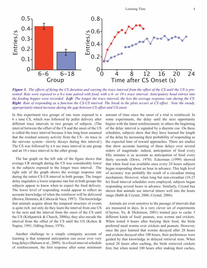
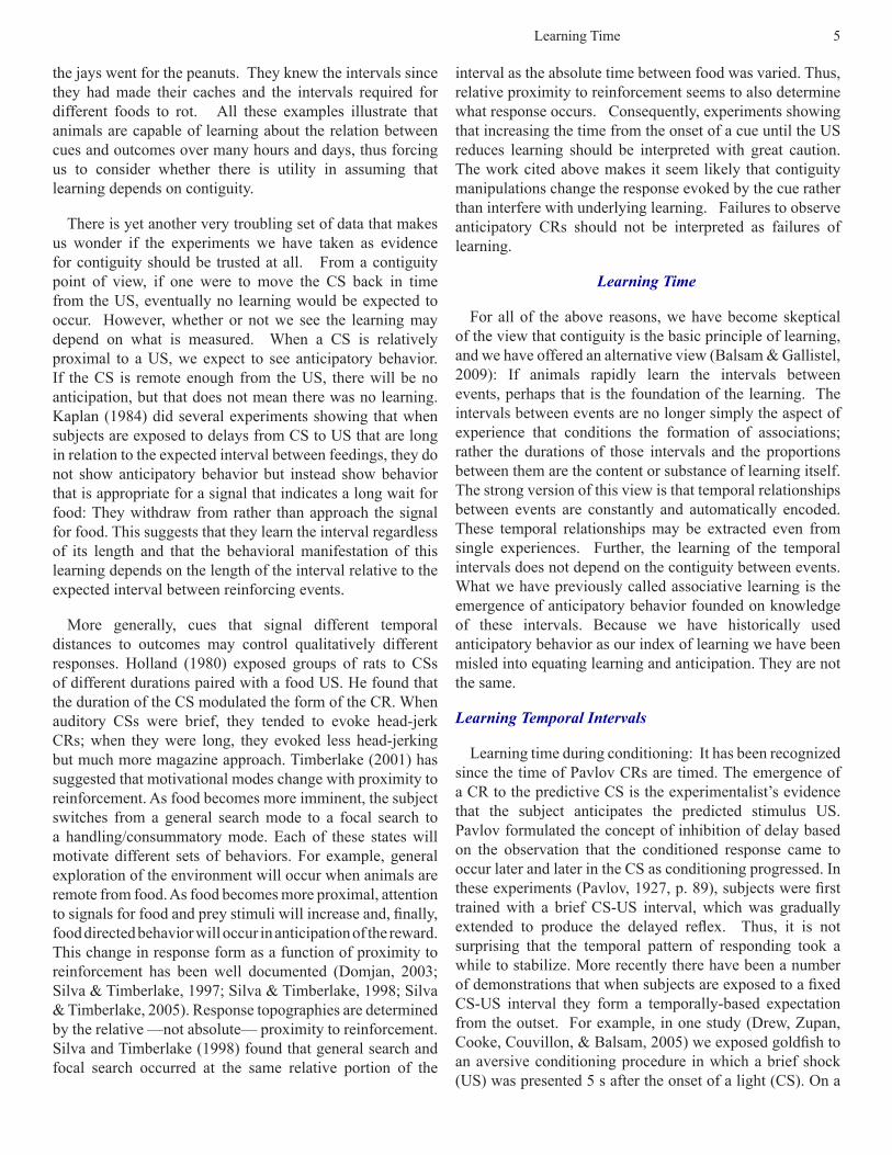
few trials in each session the light remained on for 45 s and no shock was presented. This “peak” procedure allowed us to see when the CR occurred during trials (cf. Bitterman, 1964). Figure 4 shows the development and timing of anticipatory (that is, “conditioned”) activity over the course of training. It is evident from the figure that the main effect of training is to change the magnitude of peak responding, but the time at which the CRs occur did not change. Careful modeling of the distributions over the course of training confirmed this conclusion. The peak height changes, but its location does not. Similarly, there is evidence that the very first occurrences of CRs are timed in many preparations, including eyeblink conditioning in rabbits (Ohyama & Mauk, 2001), appetitive head-poking in rats (Kirkpatrick & Church, 2000b) and autoshaping in birds (Balsam, Drew, & Yang, 2002). In fear conditioning preparations temporal control of conditioned responding can occur after just one

conditioning trial (Bevins & Ayres, 1995; Davis, Schlesinger, & Sorenson, 1989). That is, after one trial, the CR timing reflects the CS-US interval.

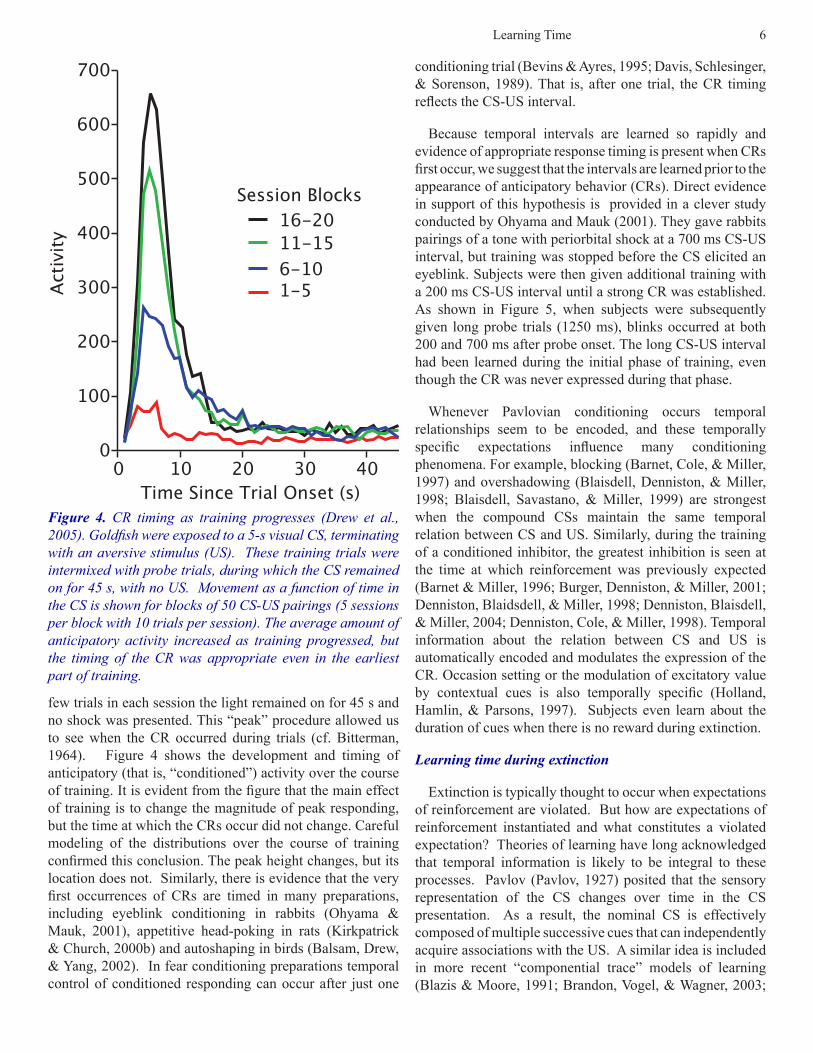
Because temporal intervals are learned so rapidly and evidence of appropriate response timing is present when CRs first occur, we suggest that the intervals are learned prior to the appearance of anticipatory behavior (CRs). Direct evidence in support of this hypothesis is provided in a clever study conducted by Ohyama and Mauk (2001). They gave rabbits pairings of a tone with periorbital shock at a 700 ms CS-US interval, but training was stopped before the CS elicited an eyeblink. Subjects were then given additional training with a 200 ms CS-US interval until a strong CR was established. As shown in Figure 5, when subjects were subsequently given long probe trials (1250 ms), blinks occurred at both 200 and 700 ms after probe onset. The long CS-US interval had been learned during the initial phase of training, even though the CR was never expressed during that phase.

Whenever Pavlovian conditioning occurs temporal relationships seem to be encoded, and these temporally specific expectations influence many conditioning phenomena. For example, blocking (Barnet, Cole, & Miller, 1997) and overshadowing (Blaisdell, Denniston, & Miller, 1998; Blaisdell, Savastano, & Miller, 1999) are strongest when the compound CSs maintain the same temporal relation between CS and US. Similarly, during the training of a conditioned inhibitor, the greatest inhibition is seen at the time at which reinforcement was previously expected (Barnet & Miller, 1996; Burger, Denniston, & Miller, 2001; Denniston, Blaidsdell, & Miller, 1998; Denniston, Blaisdell, & Miller, 2004; Denniston, Cole, & Miller, 1998). Temporal information about the relation between CS and US is automatically encoded and modulates the expression of the CR. Occasion setting or the modulation of excitatory value by contextual cues is also temporally specific (Holland, Hamlin, & Parsons, 1997). Subjects even learn about the duration of cues when there is no reward during extinction.

Learning time during extinction

Extinction is typically thought to occur when expectations of reinforcement are violated. But how are expectations of reinforcement instantiated and what constitutes a violated expectation? Theories of learning have long acknowledged that temporal information is likely to be integral to these processes. Pavlov (Pavlov, 1927) posited that the sensory representation of the CS changes over time in the CS presentation. As a result, the nominal CS is effectively composed of multiple successive cues that can independently acquire associations with the US. A similar idea is included in more recent “componential trace” models of learning (Blazis & Moore, 1991; Brandon, Vogel, & Wagner, 2003;

00 40302010

700

600

500

400

300

200

100

Activ

ity

Time Since Trial Onset (s)

1-56-1011-1516-20

Session Blocks

Figure 4. CR timing as training progresses (Drew et al., 2005). Goldfish were exposed to a 5-s visual CS, terminating with an aversive stimulus (US). These training trials were intermixed with probe trials, during which the CS remained on for 45 s, with no US. Movement as a function of time in the CS is shown for blocks of 50 CS-US pairings (5 sessions per block with 10 trials per session). The average amount of anticipatory activity increased as training progressed, but the timing of the CR was appropriate even in the earliest part of training.

Learning Time 7

Vogel, Brandon, & Wagner, 2003). According to these models, extinction should require nonreinforced exposure to the original CS duration. If subjects are trained with a CS of a given duration but extinguished with a briefer CS, little long-term extinction would be produced.

Another theory (Gallistel & Gibbon, 2000) proposes that subjects learn about the rates of the US during the CS and outside the CS. According to this theory, extinction begins when the subject decides that the US rate in the CS has changed. This decision is made by comparing the cumulative CS duration since the last US to the expected US waiting time. Thus, conditioned responding is predicted to decline as a function of cumulative exposure to the CS during extinction. This model predicts that flooding treatments, which use extended CS exposures to extinguish pathological fear in patients, will be very effective.

Recent experimental data suggest that extinction is in fact composed of two processes that are both highly sensitive to changes in the CS duration. These studies (Drew, Yang, Ohyama, & Balsam, 2004; Haselgrove & Pearce, 2003) used an experimental design in which subjects were conditioned using a fixed CS-US interval and then extinguished with CS presentations that were longer, shorter, or the same as the training CS duration. The results indicate that when the CS duration is changed between training and extinction, the loss of conditioned responding is speeded. The change in CS duration causes generalization decrement, which creates the appearance of faster extinction. Also consistent with this

interpretation is the observation that when subjects were re-exposed to the training CS duration after extinction, subjects that had received a different CS duration in extinction showed the most recovery of conditioned responding (Drew et al., 2004). That is, post-extinction responding to the training CS depended on the similarity between the extinction CS and the training CS, indicating that subjects learned the duration of the cue they experienced during extinction as well the duration of the original training cue.

In short, behavioral timing appropriate to the intervals in the training protocol is a pervasive feature of conditioned behavior. Times are learned and play an important role in learning, cue competition and extinction. In the next section we suggest that what we have called associative learning is perhaps best understood as the acquisition of temporal maps.

Temporal Maps

As animals experience the world, times are automatically encoded and stored with a temporal code that preserves the relation to other experiences. The nature of this coding of event times must be quite general, as this information can be used in very flexible ways, long after it has been encoded. For example, temporal knowledge can be integrated across experiences. This has been directly studied in higher order conditioning experiments (Arcediano, Escobar, & Miller, 2003; Barnet et al., 1997; Leising, Sawa, & Blaisdell, 2007). For example, in a sensory preconditioning experiment animals are first presented with pairings of two neutral CSs

CBA

Figure 5. Data from a single subject in an eyeblink conditioning experiment reported by Ohyama & Mauk (2001). A: Sub-ject first received CS-US pairings with a 700 ms CS-US interval. The blue part of the tracing shows the period in which the CS was presented. Note the absence of conditioned (anticipatory) blinks during this interval (the rise, that is blink onset, occurs after the blue when the US is presented). Training was stopped before subjects made anticipatory CRs. B: After the trials shown in A, the CS-US interval was reduced to 250 ms and training continued until the subject reliably blinked in anticipation of the US, as shown by these traces in which blink onset occurs during the CS (in blue). C: Traces from probe trials in which the CS remained on for 1250 ms. Subject often blinked twice, with the second blink occurring at around 700 ms. Subjects trained with only one CS-US interval did not show these double blinks.

Learning Time 8

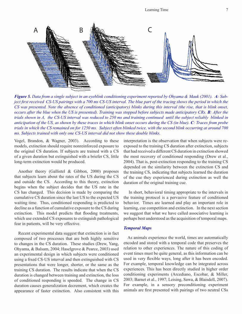
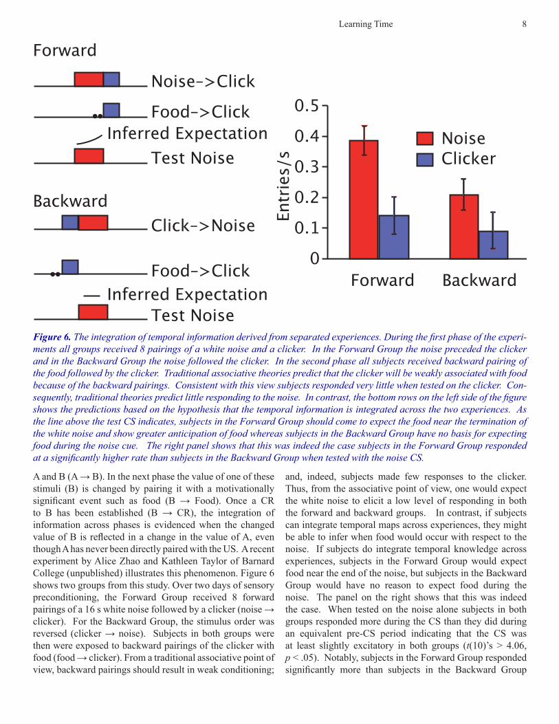
A and B (A → B). In the next phase the value of one of these stimuli (B) is changed by pairing it with a motivationally significant event such as food (B → Food). Once a CR to B has been established (B → CR), the integration of information across phases is evidenced when the changed value of B is reflected in a change in the value of A, even though A has never been directly paired with the US. A recent experiment by Alice Zhao and Kathleen Taylor of Barnard College (unpublished) illustrates this phenomenon. Figure 6 shows two groups from this study. Over two days of sensory preconditioning, the Forward Group received 8 forward pairings of a 16 s white noise followed by a clicker (noise → clicker). For the Backward Group, the stimulus order was reversed (clicker → noise). Subjects in both groups were then were exposed to backward pairings of the clicker with food (food → clicker). From a traditional associative point of view, backward pairings should result in weak conditioning;

and, indeed, subjects made few responses to the clicker. Thus, from the associative point of view, one would expect the white noise to elicit a low level of responding in both the forward and backward groups. In contrast, if subjects can integrate temporal maps across experiences, they might be able to infer when food would occur with respect to the noise. If subjects do integrate temporal knowledge across experiences, subjects in the Forward Group would expect food near the end of the noise, but subjects in the Backward Group would have no reason to expect food during the noise. The panel on the right shows that this was indeed the case. When tested on the noise alone subjects in both groups responded more during the CS than they did during an equivalent pre-CS period indicating that the CS was at least slightly excitatory in both groups (t(10)’s > 4.06, p < .05). Notably, subjects in the Forward Group responded significantly more than subjects in the Backward Group

Forward

Backward

Noise–>Click

Click–>Noise

Food–>Click

Food–>Click

Test Noise

Test Noise

Inferred Expectation

Inferred ExpectationEn

trie

s/s

0

0.1

0.2

0.3

0.4

0.5

Forward Backward

NoiseClicker

Figure 6. The integration of temporal information derived from separated experiences. During the first phase of the experi-ments all groups received 8 pairings of a white noise and a clicker. In the Forward Group the noise preceded the clicker and in the Backward Group the noise followed the clicker. In the second phase all subjects received backward pairing of the food followed by the clicker. Traditional associative theories predict that the clicker will be weakly associated with food because of the backward pairings. Consistent with this view subjects responded very little when tested on the clicker. Con-sequently, traditional theories predict little responding to the noise. In contrast, the bottom rows on the left side of the figure shows the predictions based on the hypothesis that the temporal information is integrated across the two experiences. As the line above the test CS indicates, subjects in the Forward Group should come to expect the food near the termination of the white noise and show greater anticipation of food whereas subjects in the Backward Group have no basis for expecting food during the noise cue. The right panel shows that this was indeed the case subjects in the Forward Group responded at a significantly higher rate than subjects in the Backward Group when tested with the noise CS.

Learning Time 9

(F(1, 18) = 5.67, p < .05). It should also be noted that the groups did not differ in the pre-CS rates during testing (F(1, 18) = 1.36, ns) or during first-order backward conditioning (F < 1, ns), which might have complicated interpretation of the data. Data like these as well as others (Arcediano & Miller, 2002; Wan, Djourthe, Taylor, & Balsam, 2009) document that animals can integrate temporal knowledge across experiences to make inferences about when important events will occur.

Temporal knowledge is also rapidly and continuously updated. This is evident in studies of choice, where it has been shown that rats can detect and adjust to a change in a random rate (Poisson process) as rapidly as is in principle possible (Gallistel, Mark, King, & Latham, 2001). This bears on the efficiency of temporal processing and memory because what distinguishes two random rate processes with different rate parameters is only the distribution of their inter-event intervals. These distributions always overlap, even for very different rates, because, regardless of the rate, the shorter an interval is, the more likely its occurrence. Thus, to detect a change in the rate parameter as rapidly as is in principle possible, the subject must keep track of the sequence of recent inter-event intervals and compare their distribution to the distribution expected on the hypothesis that the rate has not changed.

If temporal intervals are learned so quickly and accurately–even in the simplest of conditioning experiments–how does this knowledge guide performance? We now turn to the question of how temporal knowledge can mediate the emergence of an anticipatory response.

Temporal Information in Conditioning

The discovery of blocking and related cue-competition phenomena initially led students of traditional learning paradigms to describe the laws or principles of learning in informational terms (Rescorla, 1972). The underlying intuition was that for learning to occur a CS had to convey information about the US. Learning was driven by the correlation between the CS and the US rather than by their temporal pairing (Rescorla, 1968, 1972). Learning did not occur unless the CS conveyed new information—unless the US “surprised” the subject (Kamin, 1969a) because it was “unexpected.” There has also been some theorizing that the rewarding property of conditioned stimuli was related to the extent to which they reduced uncertainty about the delivery of primary reward (Bloomfield, 1972; Cantor & Wilson, 1981; Egger & Miller, 1962). These formulations have intuitive appeal, but they did not gain much traction because of both the resilience of contiguity-based theorizing and because there was no reason to think such processes could be instantiated in neurobiology (Clayton, Emery, & Dickinson,

2005). More recently, brain circuits that modulate learning by predictive error signals have been identified (Montague, Dayan, & Sejnowski, 1996; Montague, Hyman, & Cohen, 2004; Schultz, 2002; Takahashi et al., 2009). Thus the time seemed appropriate to rethink how an information-theoretic approach might be applied to a broad range of learning phenomena.

Information Theoretic Approach

The just-reviewed characteristics of timing and temporal memory and their role in formation of conditioned behavior form the foundation of a quantitative formulation of these intuitions (Balsam & Gallistel, 2009). The account rests on the same information-theoretic conceptual foundations as quantitative analyses of the transmission of information by sequences of action potentials (Rieke, Warland, de Ruyter van Steveninck, & Bialek, 1997). Thus it may point to a relatively direct way to map information in the world to its representation in the nervous system.

The information that a signal (for example, a CS) communicates to a receiver (the subject in a conditioning experiment) is measured by the reduction in the receiver’s uncertainty regarding the state of some stochastic aspect of the world (Shannon, 1948). The amount of information that can be communicated is limited first by the available information (source entropy, how much variation there is in that aspect of the world) and, second, by the mutual information between the signal the subject gets and the variable state of the world (roughly, the correlation between the signal received and the state of the world). The foundation of an information-theoretic analysis is the specification and quantification of the relevant uncertainties: In the present case it is the timing of the US relative to the CSs. Effective Pavlovian CSs change the subject’s uncertainty about when the next US will occur.

Variable times between events

In simple cases, the source entropy (available information) can readily be calculated. We begin by distinguishing between paradigms like the one used by Rescorla (1968), in which the CS signals a change in the rate parameter, and more conventional paradigms, in which the onset of the CS occurs at a fixed interval prior to the US.

In the experiment that Rescorla (1968) used to dissociate CS-US correlation from the temporal pairing of the CS and US, the US was generated by a random rate (Poisson) process, which is entirely characterized by the rate l (the average number of USs per unit time). Random rate processes, which make the next occurrence equally probable at any moment in time, are of special interest in analyzing temporal uncertainty

Learning Time 10

because they maximize the source entropy. For any other stochastic process there is less objective uncertainty about when the next event will occur; that is, there is less source entropy, less available information per event.

Rescorla (1968) held the US rate constant in the presence of the CS and varied the US rate in the periods when the CS was absent. Subjects developed a conditioned response to the CS, except in the critical condition, when the US rate was the same in the absence of the CS as in its presence (Figure 1). This result is not predicted by the hypothesis the temporal pairing of CS and US leads to the development of a conditioned response, because the temporal pairing between CS and US was the same in all conditions. We have previously shown that this result is predicted by considering the uncertainty about US timing in the presence and absence of the CS (Balsam & Gallistel, 2009), and we present a variant of that derivation here.

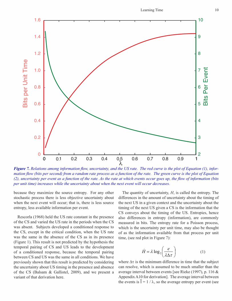
The quantity of uncertainty, H, is called the entropy. The differences in the amount of uncertainty about the timing of the next US in a given context and the uncertainty about the timing of the next US given a CS is the information that the CS conveys about the timing of the US. Entropies, hence also differences in entropy (information), are commonly measured in bits. The entropy rate for a Poisson process, which is the uncertainty per unit time, may also be thought of as the information available from that process per unit time, (see red plot in Figure 7):

D=

tll eH 2log

(1)

where Dt is the minimum difference in time that the subject can resolve, which is assumed to be much smaller than the average interval between events [see Rieke (1997), p. 116 & Appendix A10 for derivation]. The average interval between the events is I = 1 / l, so the average entropy per event (see

Figure 7. Relations among information flow, uncertainty, and the US rate. The red curve is the plot of Equation (1), infor-mation flow (bits per second) from a random rate process as a function of the rate. The green curve is the plot of Equation (2), uncertainty per event as a function of the rate. As the rate at which events occur goes up, the flow of information (bits per unit time) increases while the uncertainty about when the next event will occur decreases.

0 0.1 0.2 0.3 0.4 0.5 0.6 0.7 0.8 0.9 10

0.2

0.4

0.6

0.8

1.0

1.2

1.4

1.6

λ

Bits

per

Uni

t Tim

e

0 12

3

4

5

6

7

8

9

10

Bits

Per

Eve

nt

Learning Time 11

green plot in Figure 7) is

�

H = 1l

l log2e

lDt

= k − log2 l

(2)

where

�

k = log2e

Dt

. The difference in the per-event

entropies is:

�

H C − H CS = k − log2 lC( )− k − log2 lCS( )= log2 lCS − log2 lC

= log2 lCS lC( )= log2 I C I CS( )

where lC is the overall US rate (the context or background rate), lCS is the rate when the transient CS is also present, and IC and ICS are the reciprocals of these rates, that is, the expected intervals between USs. The critical condition in Rescorla’s (1968) experiment was the one where lCS = lC, in which case lCS/lC = 1 and HC - HCS = log2(1) = 0. In words, the presence of the CS conveys no information about the timing of the next US. Its onset does not increase the flow of information.

The Rescorla (1968) result has often been analyzed in terms of the conditional probabilities of the US in the presence and absence of the CS, but such an analysis is incomplete. Differences in rates cannot be straightforwardly reduced to differences in conditional probabilities, because there may be more than one occurrence of the US during a single occurrence of the CS. More importantly, an analysis in terms of differences in conditional probabilities does not reveal the critical role of the relative temporal intervals in the strength of the CR, nor does it clarify the meaning of contiguity.

The unusual methodology in Rescorla’s (1968) experiments calls attention to unresolved problems in specifying what constitutes temporal pairing. Traditionally, two stimuli are regarded as temporally paired when their onset asynchrony (the CS-US interval) falls within a window of associability (Gluck & Thompson, 1987; Hawkins & Kandel, 1984). However, there has been a longstanding inability to specify what that window is (Rescorla, 1972; Rescorla & Wagner, 1972). In the Rescorla (1968) experiment, unlike in most Pavlovian conditioning experiments, the temporal interval between CS onset and the US was not fixed; USs could and did occur at any time after CS onset —near the onset, in the middle of the CS or near its end. And, more than one US could occur within a single CS. This highlights the unanswered questions of where in time to position a window of associability relative to CS onset, how wide to make it, and what to do when there is more than one US within a

single such window.

The difficulty of quantifying contiguity is also evident in studies of contextual learning. When subjects learn about CSs, they simultaneously learn about contexts: they become conditioned to the experimental chamber itself (Balsam, 1985). Contextual learning, also known as background conditioning, has become an important part of modern associative theorizing. So far as we know, no one has attempted to say how it could be understood in terms of a window of associability (Colwill, Absher, & Roberts, 1988), because a single experience of the chamber (one experimental session) encompasses many USs occurring at unpredictable intervals. The “CS” (the chamber itself) may last an hour or more, with many USs during that single CS. In short, at this time, there is no rigorously formulated notion of temporal pairing, despite the fundamental role that the notion of temporal pairing plays in associative theory.

If conditioning is seen as driven by the change that a CS produces in a subject’s uncertainty about the timing of the next US, there is no longer a theoretical problem. We have already seen that a simple formal development applies to the case in which the rate of US occurrence is conditioned on the presence or absence of the CS. The same analysis explains background conditioning, because placement in the experimental chamber changes the expected rate of US occurrence, hence, the subject’s uncertainty about when the next US will occur. More formally, the per-event entropy, conditioned on the subject’s being in the chamber, is less than the unconditioned per-event entropy over the course of days or longer (Balsam, 1985). Put yet another way, the flow of information from this random rate process increases when the subject is placed in the context where that process operates. We would expect the strength of anticipatory responding controlled by a context to be a function of the overall US rate in the context, and the empirical data are consistent with this expectation (Mustaca, Gabelli, Balsam, & Papini, 1991). Thus, the information-theoretic analysis readily applies to paradigms in which the US occurs repeatedly within a single occurrence of the CS and/or there is no fixed interval between CS onset and US onset, cases in which temporal pairing, as traditionally understood, is undefined.

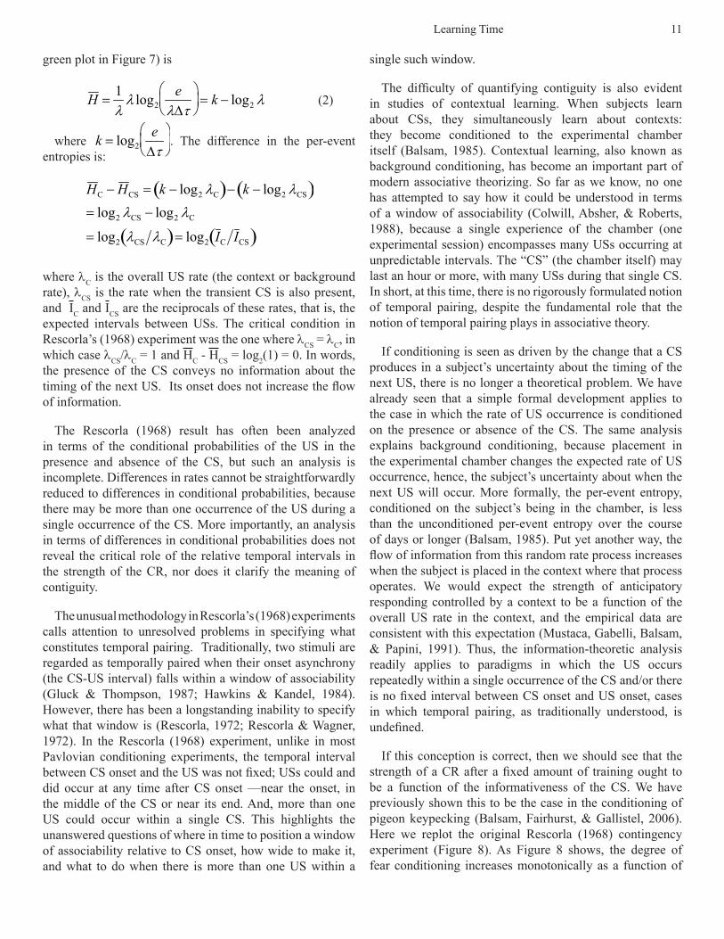
If this conception is correct, then we should see that the strength of a CR after a fixed amount of training ought to be a function of the informativeness of the CS. We have previously shown this to be the case in the conditioning of pigeon keypecking (Balsam, Fairhurst, & Gallistel, 2006). Here we replot the original Rescorla (1968) contingency experiment (Figure 8). As Figure 8 shows, the degree of fear conditioning increases monotonically as a function of

Learning Time 12

the bits of information conveyed by the CS. An additional implication of this view is that adding unsignaled reinforcers in the ITI is no more detrimental than the effects of massing trials, so long as the overall reinforcement rates are equivalent (Balsam, Fairhurst & Gallistel, 2006). Jenkins, Barnes & Berrera (1981) reported such a finding. In that experiment (Experiment 13), the percentage of ITI reinforcers preceded by the autoshaping cue was varied from 3 to 100%. All subjects that acquired keypecking did so after the same number of CS-US pairings. This is consistent with the view that the detrimental effect of adding reinforcers to the ITI is mediated by changes in background reinforcement rate.

One apparent contradiction to this conclusion comes from studies in which the ITI reinforcers are signaled by a cue that is different than the target cue (Durlach, 1983; Rescorla, 1972). If only the overall rate of reinforcement modulated acquisition it would not matter if the added reinforcers were unsignaled, signaled by the target cue (as in the Jenkins experiment), or signaled by a different cue. However, signaling the ITI reinforcers with a different cue does not decrement responding to the same extent as unsignaled US’s (Cooper, Aronson, Balsam, & Gibbon, 1990; Durlach, 1983; Rescorla, 1972). To deal with this effect Cooper et al. (1990) posited that when the ITI cue and target cue differ the two experiences are segregated. The differently signaled ITI reinforcers do not enter into the calculation of the overall rate for the target and the target reinforcers do not enter into the calculation for the alternative cue. Though the segregation of event streams into different representations was an appealing idea it did not follow in a principled way from any theoretical formulation.

The information theoretic analysis offers a principled account of these results by rationalizing the more or less arbitrary features of the Rescorla-Wagner formulation. The

essential assumptions in the Rescorla-Wagner formulation are that associations combine additively and that their combined strength reduces the potential for further associative growth, because there is an upper limit on the sum of associative strengths. These assumptions are arbitrary in that nothing about the concept of associative strength, as traditionally understood, suggests that summing associative strengths is a meaningful operation or that there should be an upper limit on the sum (which is not itself an associative strength). By contrast, in the information theoretic formulation, the source entropy of the context (the amount of uncertainty per unit time regarding the next occurrence of the US) constitutes an objective limit on the amount of information about US timing that can be provided by all sources of information combined; they cannot provide more information than is available. And, entropies add. Thus, the information about US timing provided by, for example, the experimental context, is diminished when events that occur within that context provide more of the same information. If those events together provide more information about US timing than is available from the context, then the context directly provides no information about US timing. It does provide information indirectly, by reducing uncertainty about the time to the next occurrence of the predictive CSs. This, we assume, accounts for second order conditioning and secondary reinforcement. In summary, the flow of information from the US-generating process is attributed to the stimuli that signal its operation.

Rate Estimation Theory (RET; Gallistel & Gibbon, 2000), which is similar in spirit to the present proposal, demonstrated that these properties—additivity with an inherent upper limit on the sum— suffice to explain why, for example, providing a second CS that predicts the USs not predicted by the first CS “rescues” the first CS in Rescorla’s truly random control (Durlach, 1983)—see Figure 9. In RET,

0

0

0.6

0.5

0.4

0.3

0.2

0.1

0.5 1.0 1.5 2.0 2.5Bits

Sup

pre

sio

n R

atio

.1-.1

.2-.2

.4-.4

.4-.2

.4-.1

.4-0

.2-0

.1-0

.2-.1

Figure 8. The average suppression ratios for the experimental groups in which contingency was manipulated (Rescorla, 1968). The suppression ratios are plotted as a function of the bits of information that the CS conveys about the time of expected US presentation. The regression line, Y= -0.16X + 0.47, accounts for 88% of the variance. The number pairs by each datum give the lCS and lITI for the group of subject from with the datum comes (in USs/2 minutes)

Learning Time 13

what combines additively are the rates of US occurrence predicted by different CSs (including the context). The upper limit is imposed by the fact that the sum of the rates ascribed to two or more predictors must equal the rates observed during periods when predictors are simultaneously present. A spreadsheet implementation of RET (Gallistel, 1992) is available from CRG. Readers may use it to verify that it does predict the Durlach (1983) result. The present formulation predicts the result for the same reasons, as we now explain.

We see from Equation (1) above (see also Figure 7) that the flow of information increases as the estimated rate of US occurrence increases. Information-conveying power accrues to a CS (to a potential predictor) insofar as the rate of information flow increases when that CS comes on. The accrual of information to one predictor comes at the expense of other competing predictors, because information (differences in entropy), like entropy itself, is both additive and limited by the available information. Thus, when the flow of information from the US-generating process is attributed to a transient CS, the flow attributed to the continuously present context is necessarily reduced. In Rescorla’s truly random control, the flow of information does not increase when the transient CS comes on; thus, none of the flow is attributed to it. In Durlach’s protocol, the flow of information increases dramatically when the non-target CS comes on (Figure 9, white CS). The resulting ascription of a high flow of information to the non-target CS must come at the

expense of the simultaneously present context, reducing the flow ascribed to the context. But the information flow during the target CS is not affected (Figure 9, gray CS); the rate when the target CS (and the context) are present is the same as in Rescorla’s truly random control condition. Therefore, the information flow when the target CS comes on increases above that ascribed to the context, and this increase is ascribed to the target CS. In short, the non-target CS rescues the target CS by reducing the information flow ascribed to the context.

As we have already noted, the information-theoretic explanation of cue competition phenomena rests on similar mathematical foundations (additivity under a limit) as does the explanations offered by the Rescorla-Wagner formulation and by RET. Unlike them, it gives an empirically supported definition of the elusive notion of “temporal contiguity,” as we now explain.

Fixed times between events

We consider now the application of an information-theoretic analysis to the traditional temporal pairing case, in which the US occurs a fixed time after CS onset. We assume a random rate of US occurrence while the subject is in the apparatus (hence, a variable intertrial interval), with an expected (average) interval between USs in that context of IC = 1/lC.

Truly Random

ITI USs Signaled

Effective Event Stream

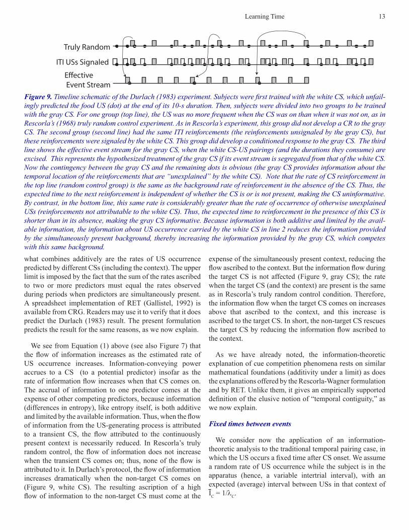
Figure 9. Timeline schematic of the Durlach (1983) experiment. Subjects were first trained with the white CS, which unfail-ingly predicted the food US (dot) at the end of its 10-s duration. Then, subjects were divided into two groups to be trained with the gray CS. For one group (top line), the US was no more frequent when the CS was on than when it was not on, as in Rescorla’s (1968) truly random control experiment. As in Rescorla’s experiment, this group did not develop a CR to the gray CS. The second group (second line) had the same ITI reinforcements (the reinforcements unsignaled by the gray CS), but these reinforcements were signaled by the white CS. This group did develop a conditioned response to the gray CS. The third line shows the effective event stream for the gray CS, when the white CS-US pairings (and the durations they consume) are excised. This represents the hypothesized treatment of the gray CS if its event stream is segregated from that of the white CS. Now the contingency between the gray CS and the remaining dots is obvious (the gray CS provides information about the temporal location of the reinforcements that are “unexplained” by the white CS). Note that the rate of CS reinforcement in the top line (random control group) is the same as the background rate of reinforcement in the absence of the CS. Thus, the expected time to the next reinforcement is independent of whether the CS is or is not present, making the CS uninformative. By contrast, in the bottom line, this same rate is considerably greater than the rate of occurrence of otherwise unexplained USs (reinforcements not attributable to the white CS). Thus, the expected time to reinforcement in the presence of this CS is shorter than in its absence, making the gray CS informative. Because information is both additive and limited by the avail-able information, the information about US occurrence carried by the white CS in line 2 reduces the information provided by the simultaneously present background, thereby increasing the information provided by the gray CS, which competes with this same background.

Learning Time 14

In the traditional temporal-pairing paradigm, the presence of a CS does not in one sense change the US rate. A subject that could not perceive the CS would detect no changes in US rate in this paradigm, whereas in some of Rescorla’s conditions, a subject that could not perceive the CS might nonetheless detect the changes in the US rate. (It might detect the otherwise undetectable presence of the CS by detecting the change in the US rate during the CS.) In the more traditional paradigm, the CS does not signal a change in rate; it signals when the US will occur, because each occurrence of the US is preceded by a CS of fixed duration, T, whose termination coincides with the US. If, however, the signaled interval is appreciably shorter than the otherwise expected interval to the next US, the CS does signal an apparent change in rate.

Given the empirically well established scalar uncertainty in subjects’ representation of temporal intervals (Gibbon, 1977), we assume that after CS onset a subject’s probability distribution for the time at which the US will occur is a Gaussian distribution with s = wT , where w is the Weber fraction (coefficient of variation) and T is the duration of the CS-US interval – see the plot of the subject uncertainty about te in Figure 11. The experimental value for w, based on the coefficient of variation in the stop times in the peak procedure, is about 0.16. It is surprisingly constant for widely differing values of T and subject species (Gallistel, King, & McDonald, 2004). The entropy of a Gaussian distribution is:

�

H =12

log2 2πe s 2

Dt( )2

Substituting wT for s and expanding, we obtain an expression for the subject’s uncertainty about the timing of the next US after CS onset.

�

H =12

log2 2πewT( )2

Dt 2

=

12

log2 2πe

+12

log2 w2 +12

log2 T 2 +12

log21

Dt

2

=12

log2 2πe + log2 T + log2 w + log21

Dt

=12

log2 2πe + log2 T + log2 w − log2 Dt( )

Equation (2), when written in terms of IC rather than lC, is

�

H C = log2e

DtI C

= log2 e + log2 I C − log2 Dt

The difference between this background uncertainty and the uncertainty immediately after CS onset is

�

log2 e + log2 I C − log2 Dt( )−

12

log2 2πe + log2 T + log2 w − log2 Dt

= log2 e + log2 I C −12

log2 2π −12

log2 e

−log2 T − log2 w

=12

log2 e − log2 2π( )+ log2 I C − log2 T − log2 w

= log2IC

T

+ k

(3)

where k =12

log2e

2π

− logw .

Equation (3) gives the intuitively obvious result that the closer CS onset is to the US, the more it reduces the subject’s uncertainty about when the US will occur. We suggest that this intuition is what underlies the widespread but erroneous conviction that temporal pairing is an essential feature of conditioning. Importantly, Equation (3) shows that closeness is relative. What matters is not the duration of T, the CS-US interval, but rather IC/T, the CS-US interval relative to the average US-US interval. This explains why it is impossible to define a window of associability —that is, a range of CS–US intervals that support associative learning. There is no such window. The relevant quantity is a unitless proportion, not an interval. Moreover, there is no critical value for this proportion. Rather, the empirically determined “associability” of the CS and US is strictly proportional to the IC/T ratio, as we now explain. (In what follows, we define and use “associability” in a purely operational sense, without commitment to the hypothesis that there is an underlying associative connection, if by “associative connection” one understands a signal-conducting pathway whose conductance depends on past experience.)

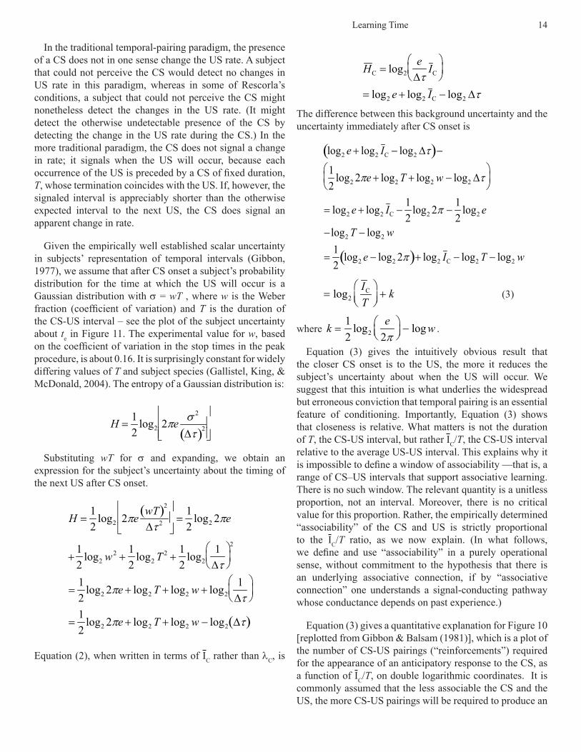
Equation (3) gives a quantitative explanation for Figure 10 [replotted from Gibbon & Balsam (1981)], which is a plot of the number of CS-US pairings (“reinforcements”) required for the appearance of an anticipatory response to the CS, as a function of IC/T, on double logarithmic coordinates. It is commonly assumed that the less associable the CS and the US, the more CS-US pairings will be required to produce an

Learning Time 15

anticipatory response. We make this assumption quantitative by assuming A = 1/NCS-US, where A = associability and NCS-US = the number of “reinforcements” (CS-US pairings) required before we observe an anticipatory response. Equation (3) says that the unitless ratio IC/T (the ratio of the average US-US interval to the average CS-US interval) is the protocol parameter that determines the amount of information that CS onset conveys about US timing. (The other relevant parameter is w, the measure of the precision with which a subject can represent a temporal interval.) This is the same quantity as IC/ ICS, which proved to be critical in analyzing the information content of the CS in the Rescorla paradigm. We call this ratio the informativeness of the CS-US relation.

Figure 10 is a plot of log(NCS-US) against log(IC/T). Remarkably, its slope is approximately -1. Thus, empirically -logNCS-US = log(IC/ICS) = log(IC/T). Taking antilogs,

1 NCS-US = A ∝ IC ICS . In words, operationally defined associability is proportional to informativeness.

Our approach to the operational definition of associability parallels the strategy in which the sensitivity of a sensory mechanism is defined to be the reciprocal of the stimulus intensity required to produce a response (as, for example, in the determination of the scotopic spectral sensitivity curve or the spatial and/or modulation transfer functions in visual psychophysics). Our analog to the required stimulus intensity is the required number of reinforcements; our operational definition of associability as the reciprocal of the required number of pairings is the analog of sensitivity (the reciprocal of required intensity). In an associative conceptual framework, the associability is the rate of learning. In our framework, associability is the speed with which a behavioral response to a predictive relation emerges: the stronger the predictive relation between cue and consequence, the fewer repetitions of the experience are required before the subject decides to respond to it. In the usual Pavlovian experiment associability is the speed with which the subject decides that an anticipatory response is appropriate for a particular temporal arrangement of events.

Consider next the case in which we let US function as its own CS by fixing , the US-US interval. In this case, it is the preceding US that enables the subject to anticipate when the next US will occur. Now, T = IC. The informativeness (their ratio) is now 1, so log(IC/T), and Equation (3) says that the information conveyed by the preceding US is

�

k =12

log2e

2π

− log2 w = −.6 − log2 w

(Note that for w < 1, -logw > 0)

The smaller w is (that is, the more precisely a subject can time and remember a fixed interval), the more information one US gives about the timing of the next US. For w = 0.16, k ≅ 2 fixing the US-US interval gives as much information about the timing of the next US as a 4-fold change of rate in the Rescorla paradigm. We know that subjects are sensitive to the information in a fixed US-US interval because there is an increase in anticipatory responding as the fixed interval between USs elapses (Kirkpatrick & Church, 2000a; Pavlov, 1927; Staddon & Higa, 1993). Sensitivity to fixed inter-reinforcement intervals is also apparent in the well known increased likelihood of responding in anticipation of the next reward, which is seen in fixed interval operant conditioning schedules (Ferster & Skinner, 1957; Gibbon et al., 1977). In an important set of experiments conducted in Doug Williams’ lab (Williams, Lawson, Cook, Mather, & Johns, 2008) subjects were exposed to a zero contingency procedure in which the rate of reinforcement in the presence of a CS was equal to the rate of reinforcement in the absence of the CS. When the CS signaled a fixed interval from its onset until US presentation, excitatory responding emerged, providing

10 1001

10

1

100

1000

IC/ T

Rei

nfor

cem

ents

to A

cqui

sitio

n ***** *

***

****

*

*****

****

*

50

20

5

2

500

200

2 5 20 50

Best Fit

95% confidence

slope = -1

Figure 10. Reinforcements to acquisition as a function of the ratio between the average US-US interval (IC) and the CS-US interval (T) on double-logarithmic coordinates. These speed-of-acquisition data come from a form of Pavlovian conditioning with pigeons called autoshaping, in which the illumination of a small circular light CS is followed by a food US. The slope of the regression is not significantly dif-ferent from -1. Based on an earlier plot (Gibbon & Balsam, 1981) with data from many different labs.

Learning Time 16

a dramatic demonstration that the information provided by fixing the CS-US interval contributes to the emergence of anticipatory conditioning beyond that contained in the simple rate ratio. The generality of such results and its consistency with quantitative information accounts remain to be explored.

CR timing

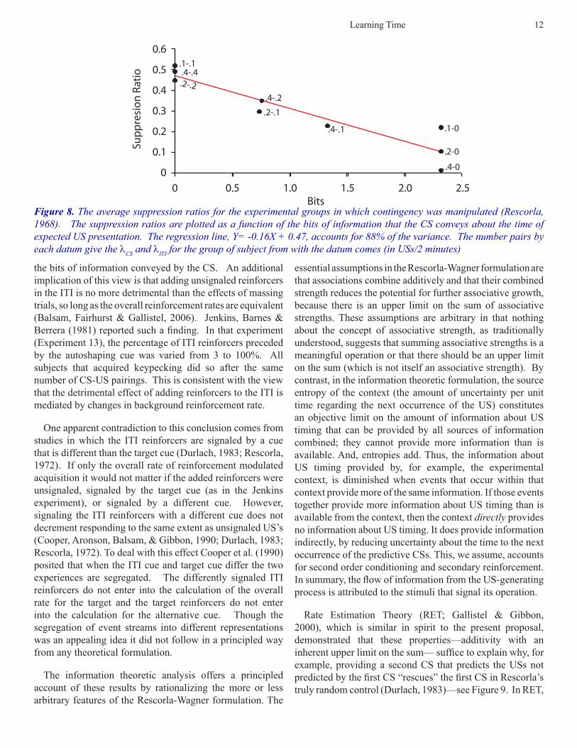
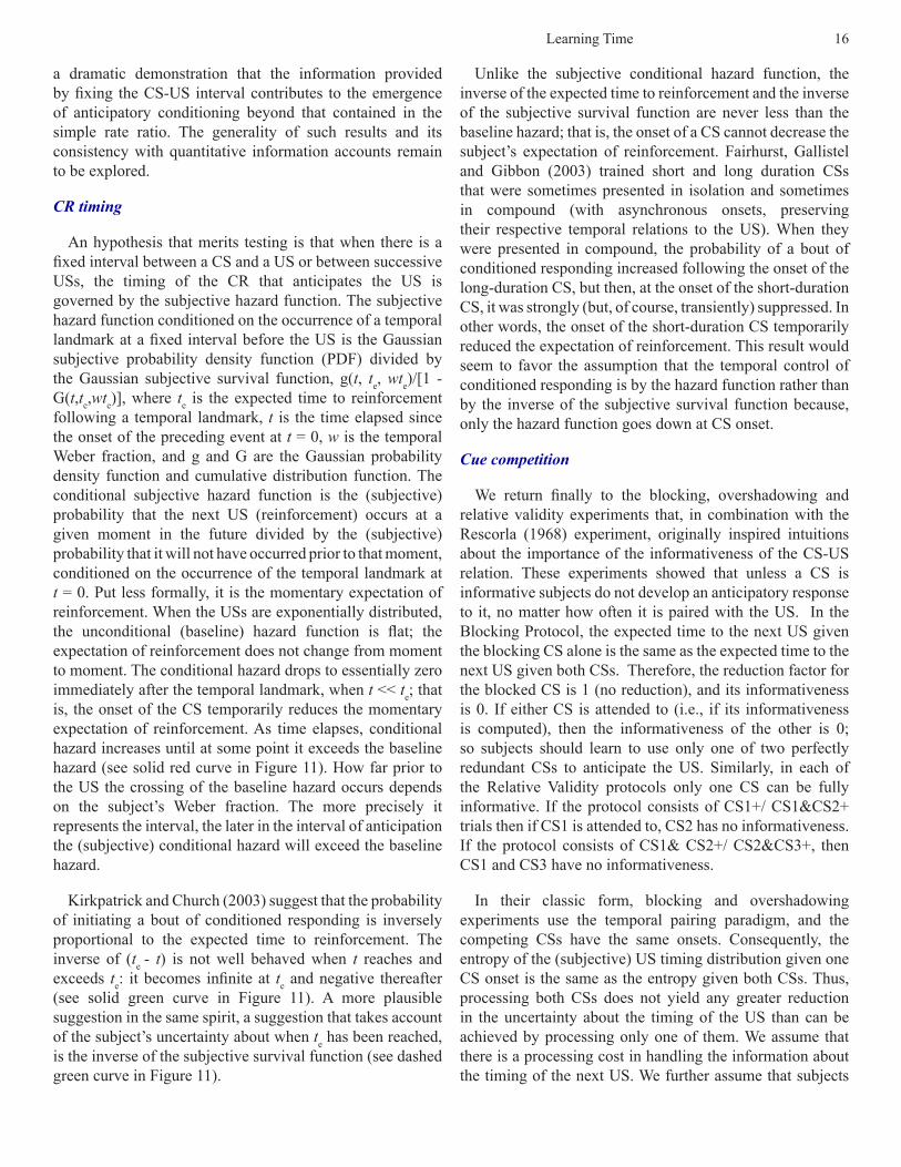
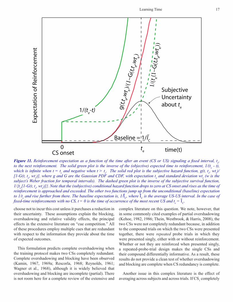
An hypothesis that merits testing is that when there is a fixed interval between a CS and a US or between successive USs, the timing of the CR that anticipates the US is governed by the subjective hazard function. The subjective hazard function conditioned on the occurrence of a temporal landmark at a fixed interval before the US is the Gaussian subjective probability density function (PDF) divided by the Gaussian subjective survival function, g(t, te, wte)/[1 - G(t,te,wte)], where te is the expected time to reinforcement following a temporal landmark, t is the time elapsed since the onset of the preceding event at t = 0, w is the temporal Weber fraction, and g and G are the Gaussian probability density function and cumulative distribution function. The conditional subjective hazard function is the (subjective) probability that the next US (reinforcement) occurs at a given moment in the future divided by the (subjective) probability that it will not have occurred prior to that moment, conditioned on the occurrence of the temporal landmark at t = 0. Put less formally, it is the momentary expectation of reinforcement. When the USs are exponentially distributed, the unconditional (baseline) hazard function is flat; the expectation of reinforcement does not change from moment to moment. The conditional hazard drops to essentially zero immediately after the temporal landmark, when t << te; that is, the onset of the CS temporarily reduces the momentary expectation of reinforcement. As time elapses, conditional hazard increases until at some point it exceeds the baseline hazard (see solid red curve in Figure 11). How far prior to the US the crossing of the baseline hazard occurs depends on the subject’s Weber fraction. The more precisely it represents the interval, the later in the interval of anticipation the (subjective) conditional hazard will exceed the baseline hazard.

Kirkpatrick and Church (2003) suggest that the probability of initiating a bout of conditioned responding is inversely proportional to the expected time to reinforcement. The inverse of (t

e - t) is not well behaved when t reaches and exceeds te: it becomes infinite at te and negative thereafter (see solid green curve in Figure 11). A more plausible suggestion in the same spirit, a suggestion that takes account of the subject’s uncertainty about when te has been reached, is the inverse of the subjective survival function (see dashed green curve in Figure 11).

Unlike the subjective conditional hazard function, the inverse of the expected time to reinforcement and the inverse of the subjective survival function are never less than the baseline hazard; that is, the onset of a CS cannot decrease the subject’s expectation of reinforcement. Fairhurst, Gallistel and Gibbon (2003) trained short and long duration CSs that were sometimes presented in isolation and sometimes in compound (with asynchronous onsets, preserving their respective temporal relations to the US). When they were presented in compound, the probability of a bout of conditioned responding increased following the onset of the long-duration CS, but then, at the onset of the short-duration CS, it was strongly (but, of course, transiently) suppressed. In other words, the onset of the short-duration CS temporarily reduced the expectation of reinforcement. This result would seem to favor the assumption that the temporal control of conditioned responding is by the hazard function rather than by the inverse of the subjective survival function because, only the hazard function goes down at CS onset.

Cue competition

We return finally to the blocking, overshadowing and relative validity experiments that, in combination with the Rescorla (1968) experiment, originally inspired intuitions about the importance of the informativeness of the CS-US relation. These experiments showed that unless a CS is informative subjects do not develop an anticipatory response to it, no matter how often it is paired with the US. In the Blocking Protocol, the expected time to the next US given the blocking CS alone is the same as the expected time to the next US given both CSs. Therefore, the reduction factor for the blocked CS is 1 (no reduction), and its informativeness is 0. If either CS is attended to (i.e., if its informativeness is computed), then the informativeness of the other is 0; so subjects should learn to use only one of two perfectly redundant CSs to anticipate the US. Similarly, in each of the Relative Validity protocols only one CS can be fully informative. If the protocol consists of CS1+/ CS1&CS2+ trials then if CS1 is attended to, CS2 has no informativeness. If the protocol consists of CS1& CS2+/ CS2&CS3+, then CS1 and CS3 have no informativeness.

In their classic form, blocking and overshadowing experiments use the temporal pairing paradigm, and the competing CSs have the same onsets. Consequently, the entropy of the (subjective) US timing distribution given one CS onset is the same as the entropy given both CSs. Thus, processing both CSs does not yield any greater reduction in the uncertainty about the timing of the US than can be achieved by processing only one of them. We assume that there is a processing cost in handling the information about the timing of the next US. We further assume that subjects

Learning Time 17

choose not to incur this cost unless it purchases a reduction in their uncertainty. These assumptions explain the blocking, overshadowing and relative validity effects, the principal effects in the extensive literature on “cue competition.” All of these procedures employ multiple cues that are redundant with respect to the information they provide about the time of expected outcomes.

This formulation predicts complete overshadowing when the training protocol makes two CSs completely redundant. Complete overshadowing and blocking have been observed (Kamin, 1967, 1969a; Rescorla, 1968; Reynolds, 1961; Wagner et al., 1968), although it is widely believed that overshadowing and blocking are incomplete (partial). There is not room here for a complete review of the extensive and

complex literature on this question. We note, however, that in some commonly cited examples of partial overshadowing (Kehoe, 1982, 1986; Thein, Westbrook, & Harris, 2008), the two CSs were not completely redundant because, in addition to the compound trials on which the two CSs were presented together, there were repeated probe trials in which they were presented singly, either with or without reinforcement. Whether or not they are reinforced when presented singly, a repeated-probe-trial design makes the single CSs and their compound differentially informative. As a result, these results do not provide a clean test of whether overshadowing and blocking are complete when CS redundancy is complete.

Another issue in this complex literature is the effect of averaging across subjects and across trials. If CS1 completely

CS onsett

e

Baseline = 1/IC

0 time(t)

SubjectiveUncertaintyabout t

e1/(t

e-t) g(

t,te

,wt e

)/(1−

G(t,

t e,w

t e)

1/(t e

(1−G

(t,t e

,wt e

))

Exp

ecta

tio

n o

f Rei

nfo

rcem

ent

Figure 11. Reinforcement expectation as a function of the time after an event (CS or US) signaling a fixed interval, te, to the next reinforcement. The solid green plot is the inverse of the (objective) expected time to reinforcement, 1/(te - t), which is infinite when t = te and negative when t > te. The solid red plot is the subjective hazard function, g(t, te, wte)/[1-G(t, te, wte)], where g and G are the Gaussian PDF and CDF, with expectation te and standard deviation wte (w is the subject’s Weber fraction for temporal intervals). The dashed green plot is the inverse of the subjective survival function, 1/{te [1-G(t, te, wte)]}. Note that the (subjective) conditional hazard function drops to zero at CS onset and rises as the time of reinforcement is approached and exceeded. The other two functions jump up from the unconditional (baseline) expectation to 1/te and rise further from there. The baseline expectation is, 1/IC, where IC is the average US-US interval. In the case of fixed-time reinforcements with no CS, t = 0 is the time of occurrence of the most recent US and te = IC.

Learning Time 18

overshadows CS2 for some subjects in a group, while for other subjects the reverse is true, the group average will imply partial overshadowing when in fact the overshadowing is complete in every subject (c.f. Reynolds, 1961). This problem is similar to the one encountered when averaging over blocks of trials before fitting an acquisition function (e.g., Thein et al., 2008) as it may give the misleading impression that the emergence of responding is continuous rather than step-like, as is often evident from an analysis of individual subjects (Balci et al., 2009; Estes, 1956; Estes & Maddox, 2005; Gallistel et al., 2004; Morris & Bouton, 2006; Papachristos & Gallistel, 2006).

Conclusion

In summary, subjects demonstrably learn the intervals in conditioning protocols, and they do so very rapidly—at or before the point at which a conditioned (anticipatory) response to the CS emerges. Furthermore, temporal relationships between events are learned even when they are measured in hours and days. Thus, temporal contiguity is not important for learning. However, relative temporal contiguity does affect the informativeness of a predictive cue (the CS in delay and trace paradigms). The informativeness of the cue affects the form and magnitude of the CR and the speed with which anticipatory CRs emerge.

The assumption that the learning of temporal relationships between events mediates the emergence of anticipatory behavior allows us to understand heretofore diverse aspects of conditioning by means of a very few intuitive principles that may be given a precise quantitative formalization. The importance of close temporal pairing (fixing a relatively short delay between CS onset and the US) and the phenomena of blocking, overshadowing, relative validity and background conditioning all follow rigorously from the intuitive idea that only CSs that inform the subject about the timing of the next US elicit anticipatory responding. More generally, we suggest that it would be best to replace the idea of learning by contiguity with the idea that learning involves extracting the temporal structure of events and the information in these structures flexibly guides the form, speed of emergence and timing of anticipation.

References

Arcediano, F., Escobar, M., & Miller, R. R. (2003). Temporal integration and temporal backward associations in human and nonhuman subjects. Learning & Behavior, 31, 242-256. PMid:14577548

Arcediano, F., & Miller, R. R. (2002). Some constraints for models of timing: A temporal coding hypothesis perspective. Learning and Motivation, 33, 105-123. doi:10.1006/lmot.2001.1102

Babb, S. J., & Crystal, J. D. (2006). Discrimination of what, when, and where is not based on time of day. Learning & Behavior, 34, 124-130. PMid:16933798

Balci, F., Gallistel, C. R., Allen, B. D., Frank, K. M., Gibson, J. M., & Brunner, D. (2009). Acquisition of peak responding: what is learned? Behavioural Processes, 80, 67-75. doi:10.1016/j.beproc.2008.09.010 PMid:18950695 PMCid:2634850

Balsam, P. D. (1985). The functions of context in learning and performance. In P. Balsam & A. Tomie (Eds.), Context and Learning. Hillsdale, N.J.: Lawrence Erlbaum Associates.

Balsam, P. D., Drew, M. R., & Yang, C. (2002). Timing at the start of associative learning. Learning and Motivation, 33, 141-155. doi:10.1006/lmot.2001.1104

Balsam, P. D., Fairhurst, S., & Gallistel, C. R. (2006). Pavlovian contingencies and temporal information. Journal of Experimental Psychology: Animal Behavior Processes, 32, 284-294. doi: PMid:16834495

Balsam, P. D., & Gallistel, C. R. (2009). Temporal maps and informativeness in associative learning. Trends in Neurosciences, 32, 73-78. doi:10.1016/j.tins.2008.10.004 PMid:19136158 PMCid:2727677

Balsam, P. D., Sanchez-Castillo, H., Taylor, K., Van Volkinburg, H., & Ward, R. D. (2009). Timing and anticipation: conceptual and methodological approaches. European Journal of Neuroscience, 30, 1749-1755. doi:10.1111/j.1460-9568.2009.06967.x PMid:19863656 PMCid:2791343

Barnet, R. C., Cole, R. P., & Miller, R. R. (1997). Temporal integration in second-order conditioning and sensory preconditioning. Animal Learning & Behavior, 25, 221-233. http://www.psychonomic.org/backissues/1007/A151.pdf

Barnet, R. C., & Miller, R. R. (1996). Temporal encoding as a determinant of inhibitory control. Learning and Motivation, 27, 73-91. doi:10.1006/lmot.1996.0005

Bevins, R. A., & Ayres, J. J. B. (1995). One-trial context fear conditioning as a function of the interstimulus interval. Animal Learning & Behavior, 23, 400-410. http://www.psychonomic.org/backissues/11/A407 corrected.pdf

Bitterman, M. E. (1964). Classical conditioning in the goldfish as a function of the Cs-Us interval. Journal of Comparative and Physiological Psychology, 58, 359-366. doi:10.1037/h0046793 PMid:14241048

Blaisdell, A. P., Denniston, J. C., & Miller, R. R. (1998). Temporal encoding as a determinant of overshadowing. Journal of Experimental Psychology: Animal Behavior Processes, 24, 72-83. doi: 10.1037/0097-7403.24.1.72 PMid:9438967

Blaisdell, A. P., Savastano, H. I., & Miller, R. R. (1999). Overshadowing of explicitly unpaired conditioned inhibition is disrupted by preexposure to the overshadowed

Learning Time 19

inhibitor. Animal Learning & Behavior, 27, 346-357. http://www.psychonomic.org/backissues/1684/A157-b.pdf

Blazis, D. E., & Moore, J. W. (1991). Conditioned stimulus duration in classical trace conditioning: test of a real-time neural network model. Behavioral Brain Research, 43, 73-78. doi:10.1016/S0166-4328(05)80054-3

Bloomfield, T. M. (1972). Reinforcement schedules: Contingency or Contiguity? In R.M. Gilbert & J.R. Milleinson (Eds.) Reinforcerment: Behavioral Analysis. NY: Academic Press, 165-208.

Brandon, S. E., Vogel, E. H., & Wagner, A. R. (2003). Stimulus representation in SOP: I. Theoretical rationalization and some implications. Behavioural Processes, 62, 5-25. doi:10.1016/S0376-6357(03)00016-0

Brown, B. L., Hemmes, N. S., & Cabeza de Vaca, S. (1997). Timing of the CS-US interval by pigeons in trace and delay autoshaping. The Quarterly Journal of Experimental Psychology B: Comparative and Physiological Psychology, 50B, 40-53. doi: 10.1080/027249997393637

Burger, D., C., Denniston, J., C., & Miller, R. R. (2001). Temporal coding in conditioned inhibition: Retardation tests. Animal Learning & Behavior, 29, 281-290. http://lb.psychonomic-journals.org/content/29/3/281.full.pdf+html

Cantor, M. B., & Wilson, J. F. (1981). Temporal uncertainty as an associative metric: Operant simulations of Pavlovian conditioning. Journal of Experimental Psychology: General, 110, 232-268. doi:10.1037/0096-3445.110.2.232

Clayton, N. S., Emery, N., & Dickinson, A. (2005). The rationality of animal memory: Complex caching strategies of western scrub jays. In S. Hurley & M. Nudds (Eds.), Rational Animals? (pp. 197-216). Oxford, U.K.: Oxford U.P.

Clayton, N. S., Yu, K., & Dickinson, A. (2001). Scrub jays (Aphelocoma coerulescens) form integrated memories of the multiple features of caching episodes. Journal of Experimental Psychology: Animal Behavior Processes, 27, 17-29. doi:10.1037/0097-7403.27.1.17 PMid:11199511

Colwill, R. M., Absher, R. A., & Roberts, M. L. (1988). Context-US learning in Aplysia californica. Journal of Neuroscience, 8, 4434-4439. PMid:3199183

Cooper, L. D., Aronson, L., Balsam, P. D., & Gibbon, J. (1990). Duration of signals for intertrial reinforcement and nonreinforcement in random control procedures. Journal of Experimental Psychology: Animal Behavior Processes, 16, 14-26. doi:10.1037/0097-7403.16.1.14 PMid:2303790

Crystal, J. D. (2006). Long-interval timing is based on a self-sustaining endogenous oscillator. Behavioural Processes, 72, 149-160. doi:10.1016/j.beproc.2006.01.010 PMid:16480835

Davis, M., Schlesinger, L. S., & Sorenson, C. A. (1989).

Temporal specificity of fear conditioning: effects of different conditioned stimulus-unconditioned stimulus intervals on the fear-potentiated startle effect. Journal of Experimental Psychology: Animal Behavior Processes, 15, 295-310. doi:10.1037/0097-7403.15.4.295 PMid:2794867

Denniston, J. C., Blaidsdell, A. P., & Miller, R. R. (1998). Temporal coding affects transfer of serial and simultaneous inhibitors. Animal Learning & Behavior, 26, 336-350. http://www.psychonomic.org/backissues/2029/A111-b.pdf

Denniston, J. C., Blaisdell, A. P., & Miller, R. R. (2004). Temporal coding in conditioned inhibition: Analysis of associative structure of inhibition. Journal of Experimental Psychology: Animal Behavior Processes, 30, 190-202. doi: 10.1037/0097-7403.30.3.190 PMid:15279510

Denniston, J. C., Cole, R. P., & Miller, R. R. (1998). The role of temporal relationships in the transfer of conditioned inhibition. Journal of Experimental Psychology: Animal Behavior Processes, 24, 200-214. doi: 10.1037/0097-7403.24.2.200 PMid:9556909

Dews, P. B. (1970). The theory of fixed-interval responding. In W. N. Schoenfeld (Ed.), The theory of reinforcement schedules (pp. 43-61). New York: Appleton-Century-Crofts.

Domjan, M. (2003). Stepping outside the box in considering the C/T ratio. Behavioural Processes, 62, pp. 103-114. doi:10.1016/S0376-6357(03)00020-2

Drew, M. R., Yang, C., Ohyama, T., & Balsam, P. D. (2004). Temporal specificity of extinction in autoshaping. Journal of Experimental Psychology: Animal Behavior Processes, 30, 163-176. doi: 10.1037/0097-7403.30.3.163 PMid:15279508

Drew, M. R., Zupan, B., Cooke, A., Couvillon, P. A., & Balsam, P. D. (2005). Temporal control of conditioned responding in goldfish. Journal of Experimental Psychology: Animal Behavior Processes, 31, 31-39. doi: 10.1037/0097-7403.31.1.31 PMid:15656725

Durlach, P. J. (1983). Effect of signaling intertrial unconditioned stimuli in autoshaping. Journal of Experimental Psychology: Animal Behavior Processes, 9, 374-389. doi:10.1037/0097-7403.9.4.374 PMid:6644244

Eckerman, D. A. (1999). Scheduling reinforcement about once a day. Behavioural Processes, 45, 101-114. doi:10.1016/S0376-6357(99)00012-1

Egger, M. D., & Miller, N. E. (1962). Secondary reinforcement in rats as a function of information value and reliability of the stimulus. Journal of Experimental Psychology: Animal Behavior Processes, 64, 97-104. doi: 10.1037/h0040364

Estes, W. K. (1956). The problem of inference from curves based on group data. Psychological Bulletin, 53, 134-140. doi:10.1037/h0045156 PMid:13297917

Learning Time 20

Estes, W. K., & Maddox, W. T. (2005). Risks of drawing inferences about cognitive processes from model fits to individual versus average performance. Psychonomic Bulletin & Review, 12, 403-408. PMid:16235625

Fairhurst, S., Gallistel, C. R., & Gibbon, J. (2003). Temporal landmarks: proximity prevails. Animal Cognition, 6, 113-120. doi: 10.1007/s10071-003-0169-8 PMid:12720110

Fanselow, M. S., & Poulos, A. M. (2005). The neuroscience of mammalian associative learning. Annual Review of Psychology, 56, 207-234. doi:10.1146/annurev.psych.56.091103.070213 PMid:15709934

Ferster, C. B., & Skinner, B. F. (1957). Schedules of reinforcement. New York: Appleton-Century-Crofts. doi:10.1037/10627-000

Gallistel, C. R. (1992). Classical conditioning as a non-stationary, multivariate time series analysis: A spreadsheet model. Behavior Research Methods, Instruments, and Computers, 24, 340-351.

Gallistel, C. R., & Gibbon, J. (2000). Time, rate, and conditioning. Psychological Review, 107, 289-344. doi:10.1037/0033-295X.107.2.289 PMid:10789198

Gallistel, C. R., King, A., & McDonald, R. (2004). Sources of variability and systematic error in mouse timing behavior. Journal of Experimental Psychology: Animal Behavior Processes, 30, 3-16. doi:10.1037/0097-7403.30.1.3 PMid:14709111

Gallistel, C. R., Mark, T. A., King, A. P., & Latham, P. E. (2001). The rat approximates an ideal detector of changes in rates of reward: implications for the law of effect. Journal of Experimental Psychology: Animal Behavior Processes, 27, 354-372. doi: 10.1037/0097-7403.27.4.354 PMid:11676086

Gibbon, J. (1977). Scalar expectancy theory and Weber’s law in animal timing. Psychological Review, 84, 279-325. doi:10.1037/0033-295X.84.3.279

Gibbon, J., Baldock, M. D., Locurto, C. M., Gold, L., & Terrace, H. S. (1977). Trial and intertrial durations in autoshaping. Journal of Experimental Psychology: Animal Behavior Processes, 3, 264-284. doi:10.1037/0097-7403.3.3.264

Gibbon, J., & Balsam, P. (1981). Spreading associations in time. In C. M. Locurto, H. S. Terrace & J. Gibbon (Eds.), Autoshaping and conditioning theory (pp. 219-253). New York: Academic.

Gluck, M. A., & Thompson, R. F. (1987). Modeling the neural substrates of associative learning and memory: a computational approach. Psychological Review, 94, 176-191. doi:10.1037/0033-295X.94.2.176 PMid:3575584

Gormezano, I., & Kehoe, E. J. (1981). Classical conditioning and the law of continguity. In P. Hazern & M. D. Zeiler (Eds.), Predictability, correlation and contiguity (pp. 1-45). New York: Wiley.

Guthrie, E. R. (1942). Conditioning: A theory of learning

in terms of stimulus, response, and association. In N. B. Henry (Ed.), The forty-first yearbook of the National Soc3iety for the Study of Education: Part II, The Psychology of Learning (pp. 17-60). Chicago, IL: University of Chicago Press University of Chicago Press Print. doi:10.1037/11335-001

Haselgrove, M., & Pearce, J. M. (2003). Facilitation of extinction by an increase or a decrease in trial duration. Journal of Experimental Psychology: Animal Behavior Processes, 29, 153-166. doi:10.1037/0097-7403.29.2.153 PMid:12735279

Hawkins, R. D., & Kandel, E. R. (1984). Is there a cell-biological alphabet for simple forms of learning? Psychological Review, 91, 375-391. doi:10.1037/0033-295X.91.3.375 PMid:6089240

Hawkins, R. D., Kandel, E. R., & Bailey, C. H. (2006). Molecular mechanisms of memory storage in Aplysia. Biological Bulletin, 210, 174-191. doi:10.2307/4134556 PMid:16801493

Holland, P. C. (1980). CS-US interval as a determinant of the form of Pavlovian appetitive conditioned responses. Journal of Experimental Psychology: Animal Behavior Processes, 6, 155-174. doi:10.1037/0097-7403.6.2.155 PMid:7373230

Holland, P. C., Hamlin, P. A., & Parsons, J. P. (1997). Temporal specificity in serial feature-positive discrimination learning. Journal of Experimental Psychology: Animal Behavior Processes, 23, 95-109. doi:10.1037/0097-7403.23.1.95 PMid:9008864

Hull, C. L. (1942). Conditioning: Outline of a systematic theory of learning. In N. B. Henry (Ed.), The forty-first yearbook of the National Society for the Study of Education: Part II, The Psychology of Learning (pp. 61-95). Chicago, IL: University of Chicago Press University of Chicago Press Print. doi:10.1037/11335-002

Jenkins, H. M., Barnes, R. A., & Berrera, F. J. (1981). Why autoshaping depends on trial spacing. In C. M. Locurto, H. S. Terrace & J. Gibbon (Eds.), Autoshaping and Conditioning Theory (pp. 255-284). New York: Academic.

Kamin, L. J. (1967). Attention-like processes in classical conditioning. In M. R. Jones (Ed.), Miami symposium on the prediction of behavior: Aversive stimulation (pp. 9-31). Coral Gables, FL: University of Miami Press.

Kamin, L. J. (1969a). Predictability, surprise, attention, and conditioning. In B. A. Campbell & R. M. Church (Eds.), Punishment and aversive behavior (pp. 276-296). New York: Appleton-Century-Crofts.

Kamin, L. J. (1969b). Selective association and conditioning. In N. J. Mackintosh & W. K. Honig (Eds.), Fundamental issues in associative learning (pp. 42-64). Halifax: Dalhousie University Press.

Kaplan, P. S. (1984). Importance of relative temporal parameters in trace autoshaping: From excitation to

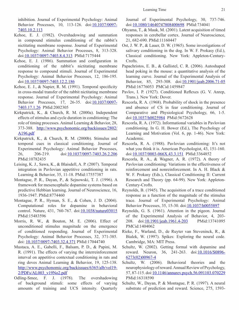
Learning Time 21

inhibition. Journal of Experimental Psychology: Animal Behavior Processes, 10, 113-126. doi:10.1037/0097-7403.10.2.113

Kehoe, E. J. (1982). Overshadowing and summation in compound stimulus conditioning of the rabbit’s nictitating membrane response. Journal of Experimental Psychology: Animal Behavior Processes, 8, 313-328. doi:10.1037/0097-7403.8.4.313 PMid:7175444

Kehoe, E. J. (1986). Summation and configuration in conditioning of the rabbit’s nictitating membrane response to compound stimuli. Journal of Experimental Psychology: Animal Behavior Processes, 12, 186-195. doi:10.1037/0097-7403.12.2.186

Kehoe, E. J., & Napier, R. M. (1991). Temporal specificity in cross-modal transfer of the rabbit nictitating membrane response. Journal of Experimental Psychology: Animal Behavior Processes, 17, 26-35. doi:10.1037/0097-7403.17.1.26 PMid:2002305

Kirkpatrick, K., & Church, R. M. (2000a). Independent effects of stimulus and cycle duration in conditioning: The role of timing processes. Animal Learning & Behavior, 28, 373-388. http://www.psychonomic.org/backissues/2802/A196.pdf

Kirkpatrick, K., & Church, R. M. (2000b). Stimulus and temporal cues in classical conditioning. Journal of Experimental Psychology: Animal Behavior Processes, 26, 206-219. doi:10.1037/0097-7403.26.2.206 PMid:10782435

Leising, K. J., Sawa, K., & Blaisdell, A. P. (2007). Temporal integration in Pavlovian appetitive conditioning in rats. Learning & Behavior, 35, 11-18. PMid:17557387

Montague, P. R., Dayan, P., & Sejnowski, T. J. (1996). A framework for mesencephalic dopamine systems based on predictive Hebbian learning. Journal of Neuroscience, 16, 1936-1947. PMid:8774460

Montague, P. R., Hyman, S. E., & Cohen, J. D. (2004). Computational roles for dopamine in behavioral control. Nature, 431, 760-767. doi:10.1038/nature03015 PMid:15483596

Morris, R. W., & Bouton, M. E. (2006). Effect of unconditioned stimulus magnitude on the emergence of conditioned responding. Journal of Experimental Psychology: Animal Behavior Processes, 32, 371-385. doi: 10.1037/0097-7403.32.4.371 PMid:17044740

Mustaca, A. E., Gabelli, F., Balsam, P. D., & Papini, M. R. (1991). The effects of varying the interreinforcement interval on appetitive contextual conditioning in rats and ring doves Animal Learning & Behavior, 19, 125-138. http://www.psychonomic.org/backissues/6365/alb/vol19-2/PDFs/AL003_v19No2.pdf

Odling-Smee, F. J. (1978). The overshadowing of background stimuli: some effects of varying amounts of training and UCS intensity. Quarterly

Journal of Experimental Psychology, 30, 737-746. doi:10.1080/14640747808400698 PMid:734041

Ohyama, T., & Mauk, M. (2001). Latent acquisition of timed responses in cerebellar cortex. Journal of Neuroscience, 21, 682-690. PMid:11160447

Ost, J. W. P., & Lauer, D. W. (1965). Some investigations of salivary conditioning in the dog. In W. F. Prokasy (Ed.), Classical conditioning. New York: Appleton-Century-Crofts.

Papachristos, E. B., & Gallistel, C. R. (2006). Autoshaped head poking in the mouse: a quantitative analysis of the learning curve. Journal of the Experimental Analysis of Behavior, 85, 293-308. doi:10.1901/jeab.2006.71-05 PMid:16776053 PMCid:1459847

Pavlov, I. P. (1927). Conditioned Reflexes (G. V. Anrep, Trans.). New York: Dover.

Rescorla, R. A. (1968). Probability of shock in the presence and absence of CS in fear conditioning. Journal of Comparative and Physiological Psychology, 66, 1-5. doi:10.1037/h0025984 PMid:5672628

Rescorla, R. A. (1972). Informational variables in Pavlovian conditioning. In G. H. Bower (Ed.), The Psychology of Learning and Motivation (Vol. 6, pp. 1-46). New York: Academic.

Rescorla, R. A. (1988). Pavlovian conditioning: It’s not what you think it is. American Psychologist, 43, 151-160. doi:10.1037/0003-066X.43.3.151 PMid:3364852

Rescorla, R. A., & Wagner, A. R. (1972). A theory of Pavlovian conditioning: Variations in the effectiveness of reinforcement and nonreinforcement. In A. H. Black & W. F. Prokasy (Eds.), Classical Conditioning II: Current Research and Theory (pp. 64-99). New York: Appleton-Century-Crofts.

Reynolds, B. (1945). The acquisition of a trace conditioned response as a function of the magnitude of the stimulus trace. Journal of Experimental Psychology: Animal Behavior Processes, 35, 15-30. doi:10.1037/h0055897

Reynolds, G. S. (1961). Attention in the pigeon. Journal of the Experimental Analysis of Behavior, 4, 203-208. doi:10.1901/jeab.1961.4-203 PMid:13741095 PMCid:1404062

Rieke, F., Warland, D., de Ruyter van Steveninck, R., & Bialek, W. (1997). Spikes: Exploring the neural code. Cambridge, MA: MIT Press.

Schultz, W. (2002). Getting formal with dopamine and reward. Neuron, 36, 241-263. doi:10.1016/S0896-6273(02)00967-4

Schultz, W. (2006). Behavioral theories and the neurophysiology of reward. Annual Review of Psychology, 57, 87-115. doi:10.1146/annurev.psych.56.091103.070229 PMid:16318590

Schultz, W., Dayan, P. & Montague, P. R. (1997). A neural substrate of prediction and reward. Science, 275, 1593-

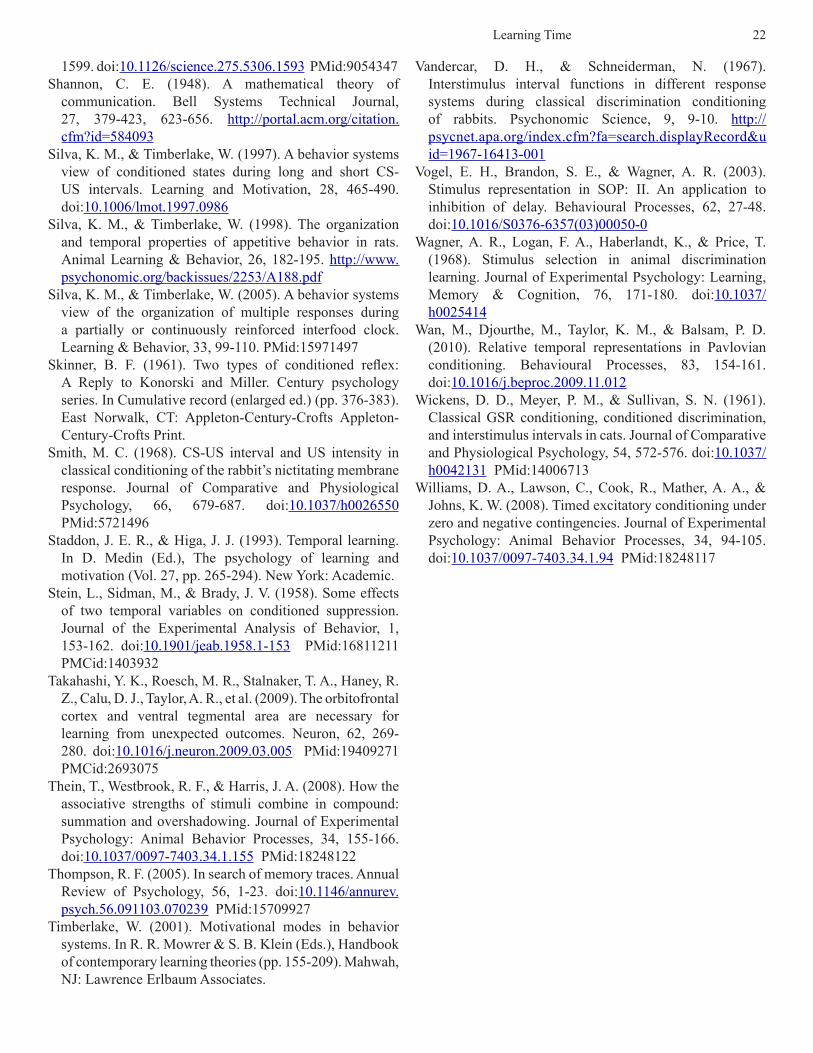
Learning Time 22

1599. doi:10.1126/science.275.5306.1593 PMid:9054347Shannon, C. E. (1948). A mathematical theory of

communication. Bell Systems Technical Journal, 27, 379-423, 623-656. http://portal.acm.org/citation.cfm?id=584093

Silva, K. M., & Timberlake, W. (1997). A behavior systems view of conditioned states during long and short CS-US intervals. Learning and Motivation, 28, 465-490. doi:10.1006/lmot.1997.0986

Silva, K. M., & Timberlake, W. (1998). The organization and temporal properties of appetitive behavior in rats. Animal Learning & Behavior, 26, 182-195. http://www.psychonomic.org/backissues/2253/A188.pdf

Silva, K. M., & Timberlake, W. (2005). A behavior systems view of the organization of multiple responses during a partially or continuously reinforced interfood clock. Learning & Behavior, 33, 99-110. PMid:15971497

Skinner, B. F. (1961). Two types of conditioned reflex: A Reply to Konorski and Miller. Century psychology series. In Cumulative record (enlarged ed.) (pp. 376-383). East Norwalk, CT: Appleton-Century-Crofts Appleton-Century-Crofts Print.

Smith, M. C. (1968). CS-US interval and US intensity in classical conditioning of the rabbit’s nictitating membrane response. Journal of Comparative and Physiological Psychology, 66, 679-687. doi:10.1037/h0026550 PMid:5721496

Staddon, J. E. R., & Higa, J. J. (1993). Temporal learning. In D. Medin (Ed.), The psychology of learning and motivation (Vol. 27, pp. 265-294). New York: Academic.

Stein, L., Sidman, M., & Brady, J. V. (1958). Some effects of two temporal variables on conditioned suppression. Journal of the Experimental Analysis of Behavior, 1, 153-162. doi:10.1901/jeab.1958.1-153 PMid:16811211 PMCid:1403932

Takahashi, Y. K., Roesch, M. R., Stalnaker, T. A., Haney, R. Z., Calu, D. J., Taylor, A. R., et al. (2009). The orbitofrontal cortex and ventral tegmental area are necessary for learning from unexpected outcomes. Neuron, 62, 269-280. doi:10.1016/j.neuron.2009.03.005 PMid:19409271 PMCid:2693075

Thein, T., Westbrook, R. F., & Harris, J. A. (2008). How the associative strengths of stimuli combine in compound: summation and overshadowing. Journal of Experimental Psychology: Animal Behavior Processes, 34, 155-166. doi:10.1037/0097-7403.34.1.155 PMid:18248122

Thompson, R. F. (2005). In search of memory traces. Annual Review of Psychology, 56, 1-23. doi:10.1146/annurev.psych.56.091103.070239 PMid:15709927

Timberlake, W. (2001). Motivational modes in behavior systems. In R. R. Mowrer & S. B. Klein (Eds.), Handbook of contemporary learning theories (pp. 155-209). Mahwah, NJ: Lawrence Erlbaum Associates.

Vandercar, D. H., & Schneiderman, N. (1967). Interstimulus interval functions in different response systems during classical discrimination conditioning of rabbits. Psychonomic Science, 9, 9-10. http://psycnet.apa.org/index.cfm?fa=search.displayRecord&uid=1967-16413-001

Vogel, E. H., Brandon, S. E., & Wagner, A. R. (2003). Stimulus representation in SOP: II. An application to inhibition of delay. Behavioural Processes, 62, 27-48. doi:10.1016/S0376-6357(03)00050-0

Wagner, A. R., Logan, F. A., Haberlandt, K., & Price, T. (1968). Stimulus selection in animal discrimination learning. Journal of Experimental Psychology: Learning, Memory & Cognition, 76, 171-180. doi:10.1037/h0025414

Wan, M., Djourthe, M., Taylor, K. M., & Balsam, P. D. (2010). Relative temporal representations in Pavlovian conditioning. Behavioural Processes, 83, 154-161. doi:10.1016/j.beproc.2009.11.012

Wickens, D. D., Meyer, P. M., & Sullivan, S. N. (1961). Classical GSR conditioning, conditioned discrimination, and interstimulus intervals in cats. Journal of Comparative and Physiological Psychology, 54, 572-576. doi:10.1037/h0042131 PMid:14006713

Williams, D. A., Lawson, C., Cook, R., Mather, A. A., & Johns, K. W. (2008). Timed excitatory conditioning under zero and negative contingencies. Journal of Experimental Psychology: Animal Behavior Processes, 34, 94-105. doi:10.1037/0097-7403.34.1.94 PMid:18248117