Embed Size (px)
Citation preview

Timberland investments in an institutional portfolio Copenhagen and Singapore, March 2013

Copenhagen and Singapore, March 2013
TIMBERLAND INVESTMENTS IN AN INSTITUTIONAL PORTFOLIO 1
Contents
EXECUTIVE SUMMARY................................................................................................ 2
1 INTRODUCTION ....................................................................................................... 4
2 TIMBERLAND RETURN CHARACTERISTICS .................................................... 4
2.1 RETURN DRIVERS ...................................................................................................... 4
2.2 RETURN STRUCTURE ................................................................................................. 6
2.3 CATASTROPHIC LOSS RISKS ...................................................................................... 8
2.4 DISTRIBUTION OF TIMBERLAND RETURNS ................................................................ 8
3 HISTORICAL TIMBERLAND PERFORMANCE ................................................. 10
3.1 TIMBERLAND PERFORMANCE INDEXES ................................................................... 11
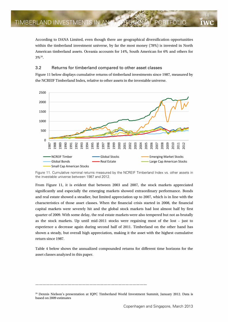
3.2 RETURNS FOR TIMBERLAND COMPARED TO OTHER ASSET CLASSES ...................... 14
3.3 CORRELATIONS OF TIMBERLAND RETURNS TO OTHER ASSET CLASSES ................. 15
3.4 PERFORMANCE MEASUREMENTS ............................................................................ 16
4 IWC’S ASSET ALLOCATION MODEL ................................................................. 19
4.1 EXPECTED RISKS, RETURNS AND CORRELATIONS ................................................... 19
4.2 EFFICIENT FRONTIER ANALYSIS ............................................................................. 20
REFERENCES ................................................................................................................ 21

Copenhagen and Singapore, March 2013
TIMBERLAND INVESTMENTS IN AN INSTITUTIONAL PORTFOLIO 2
Executive Summary
This study emphasizes the attractiveness of timberland investments for long term investors, with
good risk-adjusted returns, inflation protection characteristics, and low correlation to main
assets. Due to this range of attractive performance characteristics and diversification
opportunities from including timberland in a diversified portfolio, institutional timberland
ownership, especially in the USA, has grown significantly in the past 30 years.
The figure below displays cumulative total returns of timberland investments since 1987, as
measured by the NCREIF Timberland Index, relative to other assets in the investable universe.
Timberland has shown a steady, but overall high appreciation, making it the asset with the
highest return since 1987.
Cumulative nominal returns for timberland investment, measured by the NCREIF, relative to other assets in the investable universe between 1987 and 2012. Timberland investment returns can be described as a function of three main drivers:
Biological tree growth
Changes in timber products’ price
Changes in land value.
Ownership of timberland and the attendant biological growth, the flexibility in connection with
timing of entry/exit and timing of harvests, provide investors with an attractive return structure
as these reduce the risk of negative returns and results in a higher upside potential and a
reduced downside risk compared to investments without these characteristics.
Also, returns between professionally managed timberland investment funds are almost normally
distributed. This indicates that when investing in timberland funds, the number of investments
which needs to be made is limited in order to achieve a mean return.
0
500
1000
1500
2000
2500
1987
1988
1989
1990
1991
1992
1993
1994
1995
1996
1997
1998
1999
2000
2001
2002
2003
2004
2005
2006
2007
2008
2009
2010
2011
2012
NCREIF Timber Global Stocks Emerging Market StocksGlobal Bonds Real Estate Large Cap American StocksSmall Cap American Stocks

Copenhagen and Singapore, March 2013
TIMBERLAND INVESTMENTS IN AN INSTITUTIONAL PORTFOLIO 3
For asset allocation purposes, timberland investment return characteristics are attractive:
According to an industry index, timberland in the USA has for the period 1987 –2012
yielded a time weighted return of 12.8% p.a. nominal before asset management fee. For an internationally diversified timberland portfolio, The International Woodland Company A/S (IWC) assumes an average future nominal annual rate of return of 10% - 12% before asset management fees (returns for different strategies may vary significantly from this, e.g. investing only in the US versus investing only outside the US).
Historical standard deviation of US timberlands has been 11.3% p.a. IWC assumes an annual standard deviation of 8% - 10% for an international timberland portfolio.
Timberland returns have historically shown low or negative correlations with returns
from traditional asset classes in an institutional portfolio. IWC expects that timberland will continue to have less than perfect correlations with other asset classes.
The benefits of including timberland in an investment portfolio have been analyzed through
modern portfolio theory. IWC has produced two efficient frontiers: one that allows allocations to
timberland investments, and another where timberland is not included in the portfolio. The
results are shown in the figure below.
From the figure, it is evident that including timberland in a portfolio is beneficial as, for any
given standard deviation, the return from a portfolio including timberland is always superior.
Examples of the risk reduction by including timberland for different annual target returns are
shown in the table below. For example, if timberland is included in a portfolio with a target
return of 8.5%, the expected standard deviation can be reduced from 13.3% to 6.1% p.a.
Return Target Risk Level Change from Base Incl. Timberland
8.0% 5.6%
5.8% Excl. Timberland 11.4% Incl. Timberland
8.5% 6.1%
7.2% Excl. Timberland 13.3% Incl. Timberland
10.0% 6.7%
11.1% Excl. Timberland 17.8%
In IWC’s experience, investors typically target an allocation to timberland from between 2 to 5%
of the overall portfolio.
0%
5%
10%
15%
0% 5% 10% 15% 20% 25% 30%
Annu
al R
etur
n
Standard Deviation/Risk With Timber Without Timber TimberlandEmerging Market Stocks Global Bonds Real EstateSmall Cap American Stocks Large Cap American Stocks Global Stocks

Copenhagen and Singapore, March 2013
TIMBERLAND INVESTMENTS IN AN INSTITUTIONAL PORTFOLIO 4
1 Introduction
Institutional investments in timberland emerged in the USA in the early 1980s. Previously,
institutional ownership of timberland was limited to investments in timber product companies,
which in turn owned timberland to ensure the supply of primary resources.
As opposed to investing in timber product companies, ownership of timberland provides
investors with attractive performance characteristics.
Following the establishment of the first US-based timberland investment management
organization (TIMO) in 1981, institutional timberland investments have grown significantly.
According to AMEC Forest Industry Consulting, the investments have grown from less than USD
1 billion in 1990 to more than USD 30 billion in 20061, while DANA Limited estimates that
institutional investors have invested a total of approximately USD 60 billion as of early 20122.
Timberland Investment Resources, LLC estimated in 2011 that the global investable commercial
timberland exceeds USD 300 billion3, making it possible for the asset class to grow further in the
years to come.
Much literature has been published since the 1980s on the subject of the benefits derived from
including timberland in an institutional investment portfolio. Most of this literature is based on
US institutional investment conditions4.
In Europe, IWC has pioneered institutional timberland investments since its establishment in
1991. Particularly during the past decade, IWC has seen growing interest among European
institutional investors in international timberland investments.
This paper describes the general timberland return characteristics and the diversification
opportunities offered by including timberland in an institutional investment portfolio.
2 Timberland return characteristics
2.1 Return drivers
Timberland investment returns is often described as a function of three main drivers5 –
biological growth, change in timber prices and change in land value – as depicted in Figure 1
below.
———————————————————————————————
1 Merrill Lynch, 2007 2 Neilson, 2012
3 Chung-Hong Fu, 2012
4 Among others: Akers, 2000; Binkley et al., 1996; Caulfield, 1998a; Caulfield and Newman, 1999; Conroy and Miles, 1989; Hancock Timber Resource Group, 2003a; Redmond and Cubbage, 1988; Reinhart, 1985, Zinkhan, 1990; and Zinkhan et al., 1992 5 Caulfield, 1998b

Copenhagen and Singapore, March 2013
TIMBERLAND INVESTMENTS IN AN INSTITUTIONAL PORTFOLIO 5
Figure 1. Sources of Timberland Return6. The split between the return components can vary considerably between individual
investments. Other income sources such as higher and better use (HBU), hunting, mining
royalties, conservation easements, etc., are applicable to some investments.
Biological tree growth
Biological growth is what separates timberland from other types of investments, including
property, and it is estimated to be the most important return driver.
The effect from biological growth on return is two-dimensional. Not only do trees grow in
volume, but as they grow, they also turn into higher value products (called “ingrowth”). The
resulting extra volume and consequent value change over time are, to a large extent,
independent of macroeconomic or financial market conditions (“trees do not read the Financial
Times”).
Figure 2 below illustrates how pine trees biological growth not only provides additional volume
but higher valued products as the tree matures.
Figure 2. Sources of timberland investment returns: significance of biological growth7.
———————————————————————————————
6 RMK Timberland Group 7 IWC internal analysis
Biological growth 65-75%Timber price changes 25-30%Land value changes 2-5%
0
50
100
150
200
250
300
350
400
450
10 12 14 16 18 20 22 24 26 28 30 32 34 36 38 40 42 44 46
Volu
me
(m3/
ha)
Average DBH (cm) Pulpwood Chip & saw Sawtimber

Copenhagen and Singapore, March 2013
TIMBERLAND INVESTMENTS IN AN INSTITUTIONAL PORTFOLIO 6
Timber price change Numerous macroeconomic factors influence the price of timber, including population growth,
GDP per capita, activity in the construction sector, interest rates, and the overall level of
economic activity. Moreover, micro factors such as environmental/legacy issues affect the
stumpage price within regions8. However, it is important to note that during periods of declining
timber prices, biological growth counters the impact of reduced timber prices. Therefore,
timberland investments have a natural built-in hedge against timber price fluctuations.
Furthermore, flexibility exists when it comes to timing the harvest of trees, taking fund life,
potential leverage, etc., into account. By utilizing positive market conditions, management can
maximize the return from the investment.
Changes in land value Historically, land value only represents a small percentage of the total timberland investment
value. Land values are related to local supply and demand conditions and therefore vary
spatially. In addition, price is also partly a function of quality. Nevertheless, increasing
competition for land to be used for agriculture, bioenergy production or recreational use, as well
as for forestry, can provide major upside potential based on land appreciation9.
Furthermore, a study by Washburn10 demonstrates that the strongest indicators of real value of
land over time are the Consumer Price Index (CPI) and the nominal risk-free rate of interest.
During periods of low inflation and relative timber product price stability, timberland prices
tend to change slowly, and vice versa.
2.2 Return structure
The introduction of managerial flexibility through the ownership of timberland, as opposed to
traditional investments (e.g. into timber product companies), can be viewed as investing in two
timing options:
• Entry/exit option: Changes in the value of a timberland property are related to a number
of factors, of which changes in timber prices and presence of timber industry are
particularly important. Managers can utilize timberland market conditions when
entering and exiting the investment and thus affect the return on the investment.
• Harvest option: By utilizing market conditions and harvesting the trees when timber
prices are attractive, management can positively affect the rate of return on the
investment.
If management is assumed to maximize value and utilize varying market conditions, which
means to exercise the options optimally, the return structure of the investment will consequently
be changed.
———————————————————————————————
8 Caulfield, 1998b
9 Dasos Capital Oy, 2012 10 Washburn, 1992

Copenhagen and Singapore, March 2013
TIMBERLAND INVESTMENTS IN AN INSTITUTIONAL PORTFOLIO 7
Figure 3. The effect on return structure of introducing options or flexibility in timberland investments11. As Figure 3 illustrates, the flexibility increases the weighted average return and thus the total
return on investments. The explanation is that the flexibility makes it possible for management
to reduce unfavorable outcomes. In that respect, a timberland investment has an asymmetric
return structure, with a high upside potential and a low downside risk. Historical data, illustrated
in Figure 4 below, seem to support this. The figure compares the annual total rate of return of the
John Hancock Timber Index12 and the NCREIF13 Timberland Index with the MSCI World14 from
1970 to 2012, demonstrating the difference between volatility on the upside (positive returns)
and the downside (negative returns).
Figure 4. John Hancock Timber Index versus MSCI World15, 1970-1987, and NCREIF Timberland Index16 versus MSCI World, 1987-2012.
———————————————————————————————
11 Cordt and Degn, 2003 12 Historic timberland performance figures calculated from the John Hancock Timber Index are based on a model constructed by Hancock Timber Resource Group (HTRG), the largest timberland investment management organization (TIMO) for institutional investors. HTRG manages timberland worldwide valued at about USD 11.4 billion as of December 2012 13 National Council of Real Estate Investment Fiduciaries 14 IWC’s selected benchmark for global stocks
15 The MSCI World Equity Indices are designed to measure the performance of the global equity markets 16 Refer to section 3.1
-40%
-20%
0%
20%
40%
60%
1971
1973
1975
1977
1979
1981
1983
1985
1987
1989
1991
1993
1995
1997
1999
2001
2003
2005
2007
2009
2011
MSCI World Timberland

Copenhagen and Singapore, March 2013
TIMBERLAND INVESTMENTS IN AN INSTITUTIONAL PORTFOLIO 8
The magnitude of the positive green bars (timberland) in Figure 4 is roughly the same as the
magnitude of the positive blue bars (global stocks). In other words, the volatility on the upside is
almost similar. However, there is a significant difference on the downside: the total magnitude of
the blue bars is of completely different dimensions from the magnitude of the green bars.
The conclusion is that returns are highly elastic on the upside, but close to inelastic on the
downside for timberland investments, which is the ideal situation17.
2.3 Catastrophic loss risks
When considering the risks of timberland investments, biotic and climatic factors are often
addressed by investors. Figure 5 below indicates that professionally managed timberland has
hardly experienced adverse natural events.
Figure 5. Percentage of asset value loss out of HTRG’s entire investment pool in North America between 1992 and 201018. Less than 0.45% of the total value of the forest asset has been lost due to insects, storm, or fire in
any given year. A key point is that after a fire has hit, it is estimated that up to 90 percent of the
timber is still merchantable19.
2.4 Distribution of timberland returns
The asymmetric return structure of individual timberland investments, as described above,
should not be confused with the distribution of returns between different timberland
investments (such as institutional timberland investment funds).
If the return distribution between investments is even, the mean and median rates of return will
be identical. This implies that the number of underlying investments to be included in a
portfolio is limited in order to achieve a mean rate of return.
———————————————————————————————
17 Ineichen, 2003
18 Hancock Timber Resource Group, 2011 (the largest timberland investment management organization for institutional investors – see note 12). According to IWC’s knowledge, no such study has been conducted on the average loss outside of the United States 19 Goar, 2001
0.00%0.05%0.10%0.15%0.20%0.25%0.30%0.35%0.40%0.45%
1992
1993
1994
1995
1996
1997
1998
1999
2000
2001
2002
2003
2004
2005
2006
2007
2008
2009
2010
Fire Storm Insects/Disease

Copenhagen and Singapore, March 2013
TIMBERLAND INVESTMENTS IN AN INSTITUTIONAL PORTFOLIO 9
This is not the case when the returns of different investments are unevenly (e.g. lognormal)
distributed, where the median is lower than the mean rate of return. Under those circumstances,
the number of investments to be included in the portfolio is substantially larger. This is
illustrated in Figure 6 below.
Figure 6. Illustration of two different distributions of returns between investments20. Table 1. Distribution of annual returns of US timberland vs. US private equity/buyout funds over a 10 year period (2002-2011)21.
2002 - 2011 Mean Median Max Min Upper Lower Timberland (NCREIF) 7.6% 8.6% 19.4% -4.7% 18.5% -0.6% US Private Equity 4.7% 2.4% 491.4% -100.0% 16.5% -30.5% Table 1 above shows that compared to US private equity, the annual returns of timberland have
not only a higher mean, but also have far smaller “tails”, i.e. is platykurtic. This indicates that
extreme returns are much less likely for timberland than for investments in private equity, which
shows a distribution with larger tails, i.e. is leptokurtic. Therefore, fewer investments in
timberland will lead to a mean rate of returns.
IWC has gathered return data from 116 institutional timberland investment funds and separates
accounts investing mainly in the US. The gross IRRs are reported since inception and may
contain both realized and unrealized returns. The distribution of the return data is displayed in
Figure 7 below.
———————————————————————————————
20 Cordt and Degn, 2003 21 Data from the NCREIF Timberland Index and VentureXpert, respectively

Copenhagen and Singapore, March 2013
TIMBERLAND INVESTMENTS IN AN INSTITUTIONAL PORTFOLIO 10
Figure 7. Return distribution from 116 institutional timberland investment funds and separate accounts reported as annual gross IRR returns since inception as of 2011 year-end22. The figure shows that the distribution of the annual returns is not purely normal, nor lognormal.
This indicates that a timberland portfolio should include more than a few funds, but not as many
as when investing in private equity in order to achieve a mean rate of return.
3 Historical timberland performance
The remainder of this paper focuses on the historical and expected benefits of including
timberland investments in an institutional portfolio.
The historical data are based on reported returns between the first quarter 1987 and the fourth
quarter 2012, and the asset classes employed in the present study are the ones identified in Table
2 below.
Table 2. Asset classes and respective benchmarks used in the asset allocation study. Asset class Benchmark
Timberland Global stocks Large Cap American Stocks Small Cap American Stock Emerging Markets Stocks Global Bonds Real estate CPI Risk-free rate
NCREIF Timberland Index MSCI World Total return* SP 500* Russell 2000* MSCI EM Total Return* and ** EFFAS GBI Global Bond Series*** NCREIF Property Index US CPI LIBOR USD 3 Month
* Including reinvested dividends ** Data only dates back to 1988 *** Data only dates back to 1995
———————————————————————————————
22 IWC internal analysis 2012 based on data provided by TIMOs
05
101520253035404550
<-5%
-5-0
%
0-5%
5-10
%
10-1
5%
15-2
0%
20-2
5%
25-3
0%
30-3
5%
35-4
0%
40-4
5%
45-5
0%
50-5
5%
>55%
No
of fu
nds
Annual Return

Copenhagen and Singapore, March 2013
TIMBERLAND INVESTMENTS IN AN INSTITUTIONAL PORTFOLIO 11
The valuation of private timberland holdings is typically carried out on an annual basis by
specialists, so-called appraisers. There is no centralized auction market that continuously prices
timberland assets, not to say monitors the returns. Consequently, several analysts have designed
models of what the past performance of timberland might have been, had it been possible to
observe and record the data23.
Based on actual returns, two indices have historically reported quarterly and annual returns: the
Timberland Performance Index (TPI) and the NCREIF Timberland Index. The former was
discontinued in 1999; hence, the present study mainly uses the NCREIF Timberland Index which
is denominated in US dollars.
3.1 Timberland performance indexes
The NCREIF Timberland Index has been published since 1994 and includes returns dating back
to 1987. It is a property-based index reporting aggregated returns for the US as well as for four
regional sub-indexes (US South, Pacific Northwest, Northeast and Lake States) as of the end of
2012. The index is based on generally accepted measures of asset valuation. Additionally, the
reported income and appreciation return series conforms to theoretically appropriate concepts
of asset returns.
As of the end of 2012, the index accounted for 15 million acres of forestland (6 million hectares)
and the total value of the 443 properties was about USD 26 billion, a substantial share of
institutional timberland investments in the United States24.
However, there are at least four limitations to the NCREIF Timberland Index:
1. The number of contributing TIMOs has historically been limited and currently the index has eleven contributing members.
2. The index series only dates back to 1987, which is a relatively short period. This will be of less concern over time as more years are added.
3. The index covers only timberland investments in the United States, which as it will be shown later, is not the only market for timberland investments.
4. Only quarterly appreciation returns are reported by the NCREIF. In quarters when properties are not appraised, the appreciation is reported as zero. As a result, the quarterly return series shows a higher volatility than there actually is.
In spite of these limitations, the index is the best available measure of historical performance
and it provides some indication of expected return characteristics for timberland investments.
The annual returns for the NCREIF Timberland Index since 1987 are displayed in Figure 8 below.
———————————————————————————————
23 Binkley et al., 1996 24 NCREIF, 2012 and Washburn, 2003

Copenhagen and Singapore, March 2013
TIMBERLAND INVESTMENTS IN AN INSTITUTIONAL PORTFOLIO 12
Figure 8. Annual reported return (%/year) since 1987 for the NCREIF Timberland Index.
As it can be seen in Figure 8, timberland investments have had good historical performance. The
decomposition shows a steady, although decreasing, income return, while capital appreciation
is more volatile and has even experienced depreciation in 2001 and 2002 and again in 2009-2011.
US timberland investments have historically yielded an annual nominal return of 12.8% since
1987. The median of the returns is 11.1%, indicating a positive skewness of the annual returns.
Figure 9. Histogram of historical return p.a. since 1971 for John Hancock Timberland Index (1971-1986) and the NCREIF Timberland Index (1987-2012). Figure 9 above illustrates that there is a positive skewness in the annual timberland returns,
making a large negative return less likely than a large positive return, and a high average return,
which is in line with the overall characteristics of timberland, an attractive risk-adjusted return.
-15%-10%
-5%0%5%
10%15%20%25%30%35%
1987
1988
1989
1990
1991
1992
1993
1994
1995
1996
1997
1998
1999
2000
2001
2002
2003
2004
2005
2006
2007
2008
2009
2010
2011
2012
Income return Capital Appreciation Mean Median
012345678
(10%
) - (5
%)
(5%
) - 0
%
0% -
5%
5% -
10%
10%
- 15
%
15%
- 20
%
20%
- 25
%
25%
- 30
%
30%
- 35
%
35%
- 40
%
40%
- 45
%
45%
- 50
%
50%
- 55
%
Freq
uenc
y
Annual return

Copenhagen and Singapore, March 2013
TIMBERLAND INVESTMENTS IN AN INSTITUTIONAL PORTFOLIO 13
Figure 10. Annual reported TWRs since 1987 for the regions covered by NCREIF Timberland Index. Figure 10 shows that the annual returns vary within and between the different US regions.
Looking at the inception to date TWRs as of the end of 2012, investments in the US Northeast
yielded 7.4%, 9.6% in US South, and 16.9% in the US Pacific Northwest. The return in the Pacific
Northwest is highly impacted by positive outliers. Correcting for that by looking at the median
instead, the return is 12.6%. The Lake States region was included in the NCREIF index in 2006
and has yielded a 4.0% p.a. since inception.
As previously mentioned, a major drawback of the NCREIF Timberland Index is that it only
consists of data from the US market. For institutional investors, there are alternatives to the US
timberland market, as timberland investments outside the US are continuously getting easier to
access. This means that it is possible for investors to invest in a combination of regions that
matches investors’ preferences. HTRG has estimated annual returns since 1960 on timberland
investments in the main investable regions, based on timber prices during the prior eight
quarters. This gives an indicator of the characteristics of return in the different regions.
Table 3. Regional annual returns between 1960 to 2010 according to HTRG25.
Annual returns US South US PNW US NE Coastal
BC New
Zealand Australia Brazil
Since inception 10.4% 15.5% 8.6% 12.5% 10.6% 10.7% 17.0% Median 12.3% 12.0% 8.7% 12.1% 10.3% 13.0% 14.9% IWC considers Figure 10 as a good proxy of how the returns in the different regions have been
relative to each other. As more and more timberland investment opportunities arise in emerging
markets, like Central America, Asia, and Africa, it should be possible to achieve returns that are
above the NCREIF Timberland Index.
———————————————————————————————
25 In order to make a comparison with the NCREIF Timberland Index, as no figures exist from the outside the US prior to 1975, only returns since 1987 are used. No returns from Brazil prior to 1992 are found. Note that IWC carries out regional studies, where expected future performance, risk and correlations within geographical regions are estimated.
-20%
0%
20%
40%
60%
80%
1987
1988
1989
1990
1991
1992
1993
1994
1995
1996
1997
1998
1999
2000
2001
2002
2003
2004
2005
2006
2007
2008
2009
2010
2011
2012
South Pacific Northwest Northeast Lake States
Copenhagen and Singapore, March 2013
TIMBERLAND INVESTMENTS IN AN INSTITUTIONAL PORTFOLIO 14
According to DANA Limited, even though there are geographical diversification opportunities
within the timberland investment universe, by far the most money (78%) is invested in North
American timberland assets. Oceania accounts for 14%, South American for 6% and others for
3%26.
3.2 Returns for timberland compared to other asset classes
Figure 11 below displays cumulative returns of timberland investments since 1987, measured by
the NCREIF Timberland Index, relative to other assets in the investable universe.
Figure 11. Cumulative nominal returns measured by the NCREIF Timberland Index vs. other assets in the investable universe between 1987 and 2012. From Figure 11, it is evident that between 2003 and 2007, the stock markets appreciated
significantly and especially the emerging markets showed extraordinary performance. Bonds
and real estate showed a steadier, but limited appreciation up to 2007, which is in line with the
characteristics of those asset classes. When the financial crisis started in 2008, the financial
capital markets were severely hit and the global stock markets had lost almost half by first
quarter of 2009. With some delay, the real estate markets were also tempered but not as brutally
as the stock markets. Up until mid-2011 stocks were regaining most of the lost – just to
experience a decrease again during second half of 2011. Timberland on the other hand has
shown a steady, but overall high appreciation, making it the asset with the highest cumulative
return since 1987.
Table 4 below shows the annualized compounded returns for different time horizons for the
asset classes analyzed in this paper.
———————————————————————————————
26 Dennis Nielson’s presentation at IQPC Timberland World Investment Summit, January 2012. Data is based on 2009 estimates
0
500
1000
1500
2000
2500
1987
1988
1989
1990
1991
1992
1993
1994
1995
1996
1997
1998
1999
2000
2001
2002
2003
2004
2005
2006
2007
2008
2009
2010
2011
2012
NCREIF Timber Global Stocks Emerging Market StocksGlobal Bonds Real Estate Large Cap American StocksSmall Cap American Stocks

Copenhagen and Singapore, March 2013
TIMBERLAND INVESTMENTS IN AN INSTITUTIONAL PORTFOLIO 15
Table 4. Annualized compounded returns for the different asset classes utilized in this study as of 2012 year-end. Inception used in inception to date (ITD) return is Q1 1987.
Compounded returns
Timber-land
Global Stocks
Emerging Market Stocks
Large Cap
American Stocks
Small Cap
American Stocks
Global Bonds
Real Estate
1 year 7.75% 16.54% 18.63% 13.41% 14.63% 1.64% 10.54% 3 years 3.00% 7.53% 4.98% 8.55% 10.74% 4.66% 12.63% 5 years 2.66% -0.60% -0.61% -0.58% 2.09% 5.73% 2.13% 10 years 8.17% 8.08% 16.88% 4.95% 8.29% 5.91% 8.44% 15 years 6.57% 4.70% 9.24% 2.60% 4.53% 5.85% 9.20% 20 years 8.90% 7.39% 8.82% 6.11% 6.96% 6.06% 8.85% ITD 12.78% 7.58% 12.22% 7.06% 7.33% 6.57% 7.42% Highest 37.35% 33.76% 79.02% 34.11% 45.37% 19.01% 20.06% Lowest -5.24% -40.33% -53.18% -38.49% -34.80% -6.76% -16.85% In addition, to illustrate timberland investments’ historical attractive returns in terms of
variability characteristics, a chart of the rates of returns and standard deviations for the assets
included in the investable universe has been prepared. The rates of return and standard
deviations are based on the historical return series mentioned in Table 4. The resulting chart is
displayed in Figure 12 below.
Figure 12. Compounded annual rates of return and standard deviations of investable assets based on historical data from the 1987 to 2012. The chart clearly shows that on a historical basis, timberland investments have attractive return
and risk characteristics.
The historical data will be used as a reference point when forecasting the performance of the
asset classes. This will be developed in IWC’s Asset Allocation Model section of this report.
3.3 Correlations of timberland returns to other asset classes
Besides attractive risk and return characteristics, timberland investments have shown low
correlations with the traditional asset classes in the investable universe, which is evidently
beneficial on a portfolio basis.
Timberland
Global Stocks
Emerging Markets Stocks
Large Cap American Stocks
Small Cap American Stocks Global Bonds
Real Estate
4%5%6%7%8%9%
10%11%12%13%14%
0% 5% 10% 15% 20% 25% 30% 35% 40%
Annu
al C
ompo
unde
d re
turn
Annual standard deviation
Copenhagen and Singapore, March 2013
TIMBERLAND INVESTMENTS IN AN INSTITUTIONAL PORTFOLIO 16
Figure 13 below shows the correlations between yearly timberland returns, measured by the
NCREIF Timberland Index, and the remaining investable universe.
Figure 13. Historical yearly correlations with timberland returns between 1987 and 2012. As shown in Figure 13, timberland returns have historically correlated fairly well with inflation,
indicating that timberland investments, to some extent, provide a hedge against inflation. This is
also supported by a study made by Lutz in 2012, which concluded that a geographically
diversified timberland portfolio acts as an inflation hedge27.
Furthermore, timberland returns have correlated only slightly with most asset classes, indicating
that there are sizeable benefits to be achieved by including timberland in a diversified portfolio.
Interesting is the correlation between timberland and real estate returns which is slightly
negative. This is quite remarkable since timberland is often categorized as an alternative real
estate investment. According to the data presented in this study, there are substantial benefits to
be achieved by including timberland in a real estate portfolio28.
3.4 Performance measurements
This section encompasses a range of well-known financial key figures which are measuring the
historical performance of investable assets in different ways.
Based on the risk and return characteristics identified, the Sharpe ratio has been calculated for
each asset in the investable universe using the historical Libor 3M as the risk-free rate of return29.
Figure 14 below illustrates the result of the analysis. As shown in the figure, the excess return to
variability from timberland is attractive, and should stay so even when lowering the expected
return and increasing the standard deviation of timberland returns.
———————————————————————————————
27 Lutz, 2012 28 For more descriptions about the benefits of timberland in a real estate portfolio, see for example Hancock Timber Resource Group, 2003c; and Washburn et al., 2003 29 The Sharpe ratio is often referred to as an excess return to variability measure, and is calculated by subtracting the risk-free rate from the expected rate of return for a portfolio and dividing the result by the
standard deviation of the portfolio returns. Formula is as follows: PFP RR σ/)( −
-10% 0% 10% 20% 30% 40% 50% 60% 70%
Global Stocks
Emerging Market Stocks
Global Bonds
Real Estate
US CPI

Copenhagen and Singapore, March 2013
TIMBERLAND INVESTMENTS IN AN INSTITUTIONAL PORTFOLIO 17
Figure 14. Sharpe Ratio for each asset in the investable universe (risk-free rate of return is obtained using Libor 3M and returns are based on historical data between 1987 and 2012). In order to examine the fluctations in the Sharpe ratios over time, an analysis of each asset’s
Sharpe ratio over a 10 year horizon has been conducted, e.g. 1987-1996, 1988-1997, etc. The
outcome is shown below in Figure 15, where it is clear that the NCREIF Timberland Index
historically has not only had a high average Sharpe ratio, but also timberland investments’
lowest Sharpe ratio is significantly above those of other assets.
Figure 15. Maximum, minimum and average Sharpe Ratios for each asset class over the different 10-year periods between 1987 and 2012.
0% 10% 20% 30% 40% 50% 60% 70% 80%
Timberland
Global Stocks
Emerging Market Stocks
Large Cap American Stocks
Small Cap American Stocks
Global Bonds
Real Estate
-0.5
0.0
0.5
1.0
1.5
2.0
2.5
Timberland GlobalStocks
EmergingMarketStocks
Large CapAmerican
Stocks
Small CapAmerican
Stocks
GlobalBonds
Real Estate FTR

Copenhagen and Singapore, March 2013
TIMBERLAND INVESTMENTS IN AN INSTITUTIONAL PORTFOLIO 18
Another measure of an asset’s performance is by its alpha, which shows if an asset has yielded a
higher or lower return than forecasted according to the CAPM theory30. According to the CAPM-
theory, the return of an asset must be directly correlated to the systematic risk (the risk that
cannot be lowered by diversification). By definition, the market risk, beta (β31) of the market (in
this paper the global market32) is 1.00. A straight (β/return) line, the Security Market Line (SML),
can be drawn from the risk free rate to the market. In a perfect theoretical world, all assets should
be on this line.
Figure 16. Security Market Line and beta/return of assets. Alpha is defined as the superior/inferior return relative to the systematic risk, in other words the
vertical distance from the asset to the SML33.
Figure 17. Alpha of the investable asset classes.
———————————————————————————————
30 Capital Asset Pricing Model
31 ββasset: Cov(rasset; rmarket) / market
2
32 The market is derived based on the asset classes included in this paper, weighted with their approximate relative weight in a global portfolio. 33 αasset: rasset - βasset * rmarket
Timberland
Global Stocks
Emerging Markets Stocks
Large Cap American Stocks
Small Cap American Stocks Global Bonds
Real Estate Market
0%
2%
4%
6%
8%
10%
12%
14%
0.00 0.50 1.00 1.50 2.00 2.50
-10% -8% -6% -4% -2% 0% 2% 4% 6% 8% 10% 12%
Timberland
Global Stocks
Emerging Market Stocks
Large Cap American Stocks
Small Cap American Stocks
Global Bonds
Real Estate
σ

Copenhagen and Singapore, March 2013
TIMBERLAND INVESTMENTS IN AN INSTITUTIONAL PORTFOLIO 19
As shown in Figures 16 and 17, the performance of the historical NCREIF Timberland Index is by
far outperforming the other asset classes in this study. Even with a reduced expected
attractiveness of timberland in the future, the characteristics of timberland should remain
attractive, indicating that a superior return is expected to be so in the future as well.
4 IWC’s Asset Allocation Model
The previous sections have been focusing on historical performance, which are not in full
alignment with future performance expectations. The intention of this section is to show the
expected future benefits of timberland investments in an institutional portfolio. Therefore an
efficient frontier analysis has been carried out using expected performance for timberland and
other asset classes.
4.1 Expected risks, returns and correlations
The data needed for any asset allocation study are estimates of risk defined by the standard
deviation, rate of return, and correlation of any asset combination represented in the investable
universe.
According to IWC analysis, an international diversified timberland portfolio is expected to yield
an annual nominal rate of return of 10.6-11.1% before tax and asset management fees and an
annual standard deviation of 8.0% and 10.0%34. The remainder of the present study will employ
an expected nominal rate of return of 10% p.a. after asset management fees of 1% and an annual
standard deviation of 9.0%.
For this asset allocation study, the investable universe has been defined as: Timberland, Global
stocks, Emerging Market Stocks, Small Cap American Stocks, Large Cap American Stocks, Global
Bonds, and Real Estate. As IWC does not have the expertise to forecast expected return of other
asset classes, a study of 10-15 year expected returns, standard deviations and correlations
prepared by JP Morgan is utilized35. The resulting risks, returns, and correlations are displayed in
Table 5 below.
Table 5. Risks, returns, and correlations for the different asset classes included in the model.
———————————————————————————————
34 IWC internal analysis, 2012 35 JP Morgan Asset Management Long-term Capital Markets Return Assumptions, 2012.
Annual return 10.0% 9.5% 10.3% 9.0% 9.3% 4.3% 8.5%Standard deviation 9.0% 17.0% 27.5% 17.5% 23.0% 8.0% 13.0%
Correlation on quarterly returnsTimberland 1.00 0.05 0.07 0.07 0.06 0.05 0.06Global Stocks 1.00 0.68 0.92 0.80 -0.01 0.24Emerging Market Stocks 1.00 0.55 0.54 0.01 0.23Large Cap American Stocks 1.00 0.88 -0.15 0.20Small Cap American Stocks 1.00 -0.08 0.27Global Bonds 1.00 -0.04Real Estate 1.00
Global Bonds
Global Bonds
Real Estate
Real Estate
Global Stocks
Emerging Market Stocks
Large Cap American Stocks
Emerging Market Stocks
Large Cap American Stocks
Timberland
Timberland Global StocksSmall Cap
American Stocks
Small Cap American Stocks

Copenhagen and Singapore, March 2013
TIMBERLAND INVESTMENTS IN AN INSTITUTIONAL PORTFOLIO 20
4.2 Efficient Frontier Analysis
On the basis of IWC’s asset allocation model, two efficient frontiers have been produced: one
that allows allocations to timberland investments, and another one where timberland is
excluded from the portfolio. The results are shown in Figure 18 below.
Figure 18. Efficient frontiers including and excluding timberland investments. In Figure 18, the green curve is the efficient frontier when timberland is allowed in the portfolio
and the dashed light blue doted curve is the efficient frontier when timberland is excluded from
the portfolio. The efficient frontier is reaching a larger return for a specific risk, when including
timberland in the portfolio, indicating that allowing an allocation to timberland into a portfolio
is beneficial. This is further substantiated by the high optimal allocation to timberland.
The incremental benefits of including timberland in the portfolio are summarized in the table
below which shows the subsequent reduction of risk when including an allocation to timberland
in a diversified portfolio. As an example, the table shows that if we include an optimal allocation
to timberland in a portfolio with a target annual rate of return of 8.5%, the expected standard
deviation can be reduced from 13.3% to 6.1%.
Table 6. Incremental benefits of allowing allocation to timberland.
Return Target Risk Level Change from Base
Incl. Timberland 8.0%
5.6% 5.8%
Excl. Timberland 11.4%
Incl. Timberland 8.5%
6.1% 7.2%
Excl. Timberland 13.3%
Incl. Timberland 10.0%
6.7% 11.1%
Excl. Timberland 17.8% As a result, it is IWC’s belief that timberland investments will in the future continue to have a
positive impact on an institutional portfolio.
0%
5%
10%
15%
0% 5% 10% 15% 20% 25% 30%
Annu
al R
etur
n
Standard Deviation/Risk With Timber Without Timber TimberlandEmerging Market Stocks Global Bonds Real EstateSmall Cap American Stocks Large Cap American Stocks Global Stocks

Copenhagen and Singapore, March 2013
TIMBERLAND INVESTMENTS IN AN INSTITUTIONAL PORTFOLIO 21
References
Akers, K. (2000): Global timber investments: An important role in intuitional portfolios – Paper
from UBS Asset Management, UBS Timber Investors Research, September 2000.
Binkley, C.S., C.F. Raper, and C.L. Washburn (1996): Institutional ownership of US timberland.
History, rationale and implications for forest management – Journal of Forestry 9 (Sep 1996), 21 –
28.
Caulfield, J.P. (1998a): Timberland in institutional portfolios and the question of persistence –
Forest Products Journal, Apr. 1998, 48(4), 23 – 28.
Caulfield, J.P. (1998b): Timberland return drivers and investing styles for an asset that has come
of age – Real Estate Finance, winter 1998, 14(4), 65 – 78.
Caulfield, J.P. and D.H. Newman (1999): Dealing with timberland investment risk: Theory versus
practice for institutional owners – Journal of Forest Economics 5:2 1999, 253 – 268.
Conroy, R. and M. Miles (1989): Commercial forestland in the pension portfolio: the biological
beta – Financial Analysts Journal, Vol. 45, September - October 1989, 46-54.
Cordt, L. and T. Degn (2003): Værdiansættelse af fleksibilitet – DTA eller ROV? –
Kandidatafhandling – Copenhagen Business School (Denmark, unpublished).
Dasos Capital Oy (2012): Future prospects for forest products and timberland investment.
Elton, E., and M. Gruber (1995): Modern Portfolio Theory and Investment Analysis – John Wiley
& Sons, Inc. 1995.
Goar, J. S. (2001). Into the Woods – Bloomberg Wealth Manager.
Hancock Timber Resource Group (2003a): Timberland as a portfolio diversifier – Research Notes
2003.
Hancock Timber Resource Group (2003b): The NCREIF Timberland Property Index – Research
Notes 2003.
Hancock Timber Resource Group (2003c): The benefits of timberland in a real estate portfolio,
revisited – Hancock Timber Research Note, Jun. 2003, N–03–7.
Hancock Timber Resource Group (2003d): Risk from natural hazards for timberland investments
– Hancock Timberland Investor Second Quarter 2003.
Hancock Timber Resource Group (2011): Casualty Losses in Timberland Investments– Hancock
Timberland Investor Second Quarter 2011.
Ineichen, A.M. (2003): Fireflies before the storm – UBS Warburg – AIS Report.
JPMorgan Asset Management Long-term Capital Market Return Assumptions. As of November
30 2008.

Copenhagen and Singapore, March 2013
TIMBERLAND INVESTMENTS IN AN INSTITUTIONAL PORTFOLIO 22
Lutz, J. (ed.) (1999): Measuring timberland performance – Timberland Report 1(2) James W.
Sewal Company.
Lutz, J. (2007): Inflation and Timberland Returns – Update. – Forest Research Notes. Volume 9,
Number 2, 2nd Quarter, 2012.
Merril Lynch (2007): Timber Survey: What will institutional investors do next?
Mercer (2006): Timberland as an investment for institutional portfolios. NCREIF (2008): Timberland Index Detailed Quarterly Performance Reports.
Neilson, D. DANA Limited. Timberland ownership is still only a minute proportion of the total financial market asset base, but ownership is rapidly moving from regional to global; and transaction prices continue to defy gravity -- or do they?
Redmond, C. H. and F. W. Cubbage (1988): Portfolio risk and returns from timber asset
investments – Land economics, Vol. 64(4), Nov. 1988, 325-337.
Reinhart, J. (1985): Institutional investment in U.S. timberlands – Forest Products Journal, 35(5),
13-18.
The International Woodland Company A/S (2005) Global Forestland Investment Study.
The International Woodland Company A/S (2012) Regional Allocation Model (Internal research
paper, not published).
VentureXpert. Thomson Financial.
Washburn, C., C. Binkley, and M.E. Arenow (2003): Timberland can be a useful addition to a
portfolio of commercial properties – PREA Quarterly, Summer 2003, 28 – 31.
Washburn, C.L. (1992): The Determinants of Forest Value in the U.S. South – In Proceedings of
the 1992 Southern Forest Economics Workshop, May 29, 1992.
Washburn, C.L. (2003): Personal comment. Director of Economic Research & Investment
Strategy, Hancock Timber Resource Group, 99 High Street, 26th Floor.
Zinkhan, F. C. (1990): Timberland as an Asset for Institutional Portfolios – Real Estate Review, 19,
69-74.
Zinkhan, F. C., W. R. Sizemore, G. G. Mason, and T. J. Ebner (1992): Timberland investments: a
portfolio perspective – Portland, OR, Timber Press.