Embed Size (px)
Citation preview

Tilburg University
A decision theoretic analysis of the unit root hypothesis using mixtures of ellipticalmodelsKoop, G.; Steel, M.F.J.
Publication date:1991
Link to publication in Tilburg University Research Portal
Citation for published version (APA):Koop, G., & Steel, M. F. J. (1991). A decision theoretic analysis of the unit root hypothesis using mixtures ofelliptical models. (CentER Discussion Paper; Vol. 1991-50). Unknown Publisher.
General rightsCopyright and moral rights for the publications made accessible in the public portal are retained by the authors and/or other copyright ownersand it is a condition of accessing publications that users recognise and abide by the legal requirements associated with these rights.
• Users may download and print one copy of any publication from the public portal for the purpose of private study or research. • You may not further distribute the material or use it for any profit-making activity or commercial gain • You may freely distribute the URL identifying the publication in the public portal
Take down policyIf you believe that this document breaches copyright please contact us providing details, and we will remove access to the work immediatelyand investigate your claim.
Download date: 14. Dec. 2021

~~- ~ r~R DiscussionR
for ~ ~~8414 ~mic Research1991 -i
50
P~
~
~~~~
1~~0JQ~J~ ,
1 ~~~1111119111 1111~IIIIIIIIp!I~;~I6nl
No. 9150
A DECISION THEORETIC ANALYSIS OF THE UNIT ROOTHYPOTHESIS USING MIXTURES OF ELLIPTICAL MODELS
by Gary Koopand Mark F.J. Steel
September 1991
zSSN 09z4-7815

A DECISION THEORETIC ANALYSIS OF THE UNIT ROOT
HYPOTHESIS USING MIXTURES OF ELUPTICAL MODELS
Gary KoopDepanmern of Econank:sBoston UniveraltyBoston MA 02215
and
btark F.J. SteelDepartment o( Econorn~sTMburg UnNerslryP.O. Box 901535000 LE TilburgThe Netherlands
ABSTRACT: This paper develops a formal decision theoret~ approach to testing for a unR root ineconomlc time serles. The approach fs empirk~lly knpiemented by speciíy(ng a loss function based onpredictNe variances; models are chosen so as to minimize expected kiss. In additkxt, the paperbroadens the dass of Ilkelihood functkxts tradftkxtally consklered In the Bayesian unft root Ifterature byi) allowing for departures from nomialiry via the specrtication of a Iikelihood based on general elllpticaldensftles; I~ aliowing for structural breaks to occur; lif) allowing for moving average errors; atá fv) usingmixtures of various submodels to create a very flexible overaA Iikelihood.
Acknowledgements: The first author gratefully ackrw~Medges the hospltaltty of CentER, TYburg UnNersiry,whAe the second author was supported by a resaerch fellowship of the Royal Netherlands Atstdemy ofArts and Sckjnce (KNAW). We also thank Jacek Oskiwalskl for many helpful diacussions and Hermanvan Dijk for kindly provkiing the data.
Please send correspondence to Gary Koop, London School of Economics, Houghton St., London, WC2A2AE, United Kingdom.

x
The economic Iiterature devoted to the Isaue of unlt roota in econom~ tlme serlea hea grownImmensely since the seminal papers of Dickey and Fuller (1979) and Nelson end Plosser (1982).
Although the maJorlty of the Ilterature assumes a dassk~.al econometric perspedNe, a growing Bayeslan
unR root literature has emerged (see DeJong and Whlteman (1991a,b), Phplips (1991), Sima (19tt8), Koop
(1991a,b), Schotman arxl van DI)k (1991a,b), Wago and Tsuruml (1990), ZNot and Phllllps (1991)). In
many cases, Bayeslan resufts dHfer aubstantlally from thetr dasalcal counterparts.
This paper makes a contribution to thla growing body of f3ayeslan unh root IRerature. It
consklers more general classes of models and methods of drawing inferences than presently exist. The
paper uses models that are mbdurea over varkws aubmodels wRh general elliptk~l distrlbutkxu and
differ In both thelr covariance structure and their treatmeru of stnictural breaks. The resttltkp mbced
model is very 8exible and encompasses a wide varlety of dynamk; structures. In addftkxt, the peper uses
a formal decision theoretlc fmmework based on predldNe varlances ard the conservatNe notbn that
it is worse to underestimate than to overestlmate predictNe variances. This approach accords naturally
with a Bayeslan paradlgm and provkfes an expl~k forum for choosing between stationary, unR root, and
expioslve models.
Section t of the paper Introduces our hypothesis of interest and the methodology we use to test
R. Section 2 discusses the sampling model, Sectkx~ 3 the prkx density, and Section 4 the posterbr
denstty. Section 5 treats the decislon problem whYe Sectkxt 8 applies the methods to the extended
Nelson-Plosser data set. Sectlon 7 condudes.
Sectlon 1: What Are Wa Testing?
Our aim Is to determine whether a unR root Is present, le. to test an exact restrlctlon. One
obvbus way is to calculate posterlor odds comparing the model wtth a unft root imposed agalnst the
unrestrk;ted model. This method requlres that an InformatNe (proper) prkx be placed over p, the
coeff~leru whk:h equals one under a unR root. Koop (1991a,b) calculates posterior odds using
IMormatNe natural conjugate prkxs. Schotman and van DiJk (1991a) use proper priors that requlre less
subJectNe prior Input but at the cost that their prkxs are data-based.
Rather than test explk.itly for a unft root, an aftematlve methodology (DeJong and Whiteman
(1991 a,b) and PhGlips (1991)) Is to calculate the poaterlor probabUity that p Is in some region near one.
This method has the advantage that proper prlont are no longer necessary and thus the anatysis may
be made more 'objectNe'. The disadvantage la that the definftion ot p as 'close to one' Is highly
subJectNe. By way of example, ~nsWer Phplfps (1991) wtwcalculates the probabuity that ~ p ~ x.975 and
~ p I t t. The fomier is hlghly sub)ective whereas the latter fs sultable for testing for nonstatkxtaritlea (le.
unR root or explosNe behavkx) but not for the presence oF a unit root per se. In this peper, we use
proper prkxs on p wh~h sAow us to compute posterior odds tor the exact unft root null.
Furthermore we use a decisfon theoretk: iramework to carry out the unit root tests. The loss
3
function used In the decislon analysis is based on predlctNe behavior which can differ cruclally for
stationary (H,: I v I~ 1), unlt root (H,: v-1), and axplosNe (H,: I v I~ 1) models. Hence our decislon
problem Is set up In terms of these three regkms for p.
Sectfon 2: The Likelihood Functfon
Bayeslan methods require the specificatkxt of a Ilkellhood functkxt. PhYlips (1991), for example,
bases his Iikellhood (unction on the fdlowing speclficatkxr.
M-1
Yr' Y'~'vYr-r'~~~Yr-r`~rtii
(~)
wtth c, I.i.d. N(O,i~,
whAe DeJong and Whiteman (1991a) use a dMferent parameterizatkxi. Slnce anelytir,al resulta cannot
always be obtalned for their perameterizatlon and eoctensive Morrte Carlo Integratkm Is requlred, PhYlips'
parameterizatkxi Is preferred (see PhAlips (1991)).'
We expand the dass of conskiered Ilkellhoods In three knportant dlrectlons: a) By relaxing the
normality assumptkxr b) By relaxing the I.I.d. assumption; and c) By allowing for structural breaks (Perron
(1989), Banerfee, Lumsdaine and Stock (1990) and ZNot and PhAlips (1990)). We let y(where Y- (Y,....~YT)')
have any density within the dass of multNariate elliptical densRl~, thereby covering such denskles as
the muKNarlate normal, muttNariate-t and Pearson type-Ii. Moreover, we allow the covariance matrix to
take the form t''V(q), where V(,)) fa any posltNe defkdte symmetrk; matrbc parameterized by a finite vector
q. Technlques for handling extenslons a) and b) are described In Osiewalskl and Steel (1990) and Chib
et al. (1990).
In this paper, no single model need be selected for Nnal analysis. Several dNferent stnx,tural breflks
and structures for V(p) can be chosen, and a supermodel, which is a flnite mixture of the various
submodels, used. We allow V(q) to have varkws stnictures In the ARMA dass. The motivation behind
the Induslon of a moving average componeru Is discussed in Schwert (1987).
Formalizing the kieas descrlbed In the preceding paragraphs, we begin with the model wfth rw
structural breaks (M„). We mix over m differerrt correlation struciures so that each IndNkiual model Is
labelled M„ (1-1,...,m). For each model M,~ we take:
P(y I 9MT~,~,Yp~.M„J- I r~Vw(v11-'~
9wI(Y-hw(Br.~)'T'Yia' (n) (Y-hw(eN))1(2)
' In the empirk~l sectkxi we fdlow DeJong and Whheman (1991a,b) and aet k-3.
4
where gw(.) Is a nonnegatNe functlon wh~h satisfies (for all I and T),
ruR rgw(uJClu-I'(T~2)n-r~~. (3)
In other words, we assume y has a T-variate elliptical density. Note that (3) Is a necessary and sufficientcondftion tor (2) to be a proper densfty, y~ is the vector o( Initlal observatlons (y,,, ...,y~', and hw(9,~
Is a vector of length T with property:
A-,
~hw(eN)Jr' Nt~iDyr-i~ ~~PYf-rj-~
Since we assume this function to be Identk,al for ap covarlance structures, we drop the I subscript andwrite:
hN(eNI -~Y-1 fX~N
where
iY-,'(Yo~Yi,...,Yr-i) ,
r yN ~XN-Y`t ,...XT ,
X~-(~ ,t,~y,-,,...,0 yf-A.IiI),,r
aN'W,I~,W 1....,~1-1)'- W .Y,~,,
and tlence 9N - (o, oN )'For future reference we define:
dw(er,~ ~) -(Y-hN(eN))via~ (n) (Y-hN(BN))
(4)
(5)
The model withou[ stnictural breaks ( M,,) Is then glven by the mbRUre of the probabllftles In (2)over the m covariance structures:
P(y I 9MT~,n,d,Y~,M,J
-~df P(y I 6Mt~,n,Yp,Mw)~r-,
(8)
where d -(d,,...,d„J' is a vector of mixing parameters with d,ZO and F.d,-1.
We obtain the model with structural breaks (M~ by máing over varkws covariance stnicturesQ-1,...,m) and breakpoints ( q-1,...,T-t). Note thet we use the same coverfence atructures as In the
previous model. Although not necessary, doing so slmpltFles the notatlon such that Vw-Va-Vi for IaJ.
Moreover, we conceptually allow for the structural breaks to occur at any point in our sampie. Two types
of structural breaks, level breaks and trend breaks, can occur at anytime q z 1,...,T-1. Perron (1989) arguestor the presence of a level break In 1929 and a trend break In 1973 for moet U.S. mecroeconomic time
series. To reduce the burden of computation only the latter two breaks are Included in the empirk~i
analysis aithough the general notation is retained throughout this section.
5
Me Is a mlxture over models wRh dlfterern structural breakpolnts and covarlance structures (M~.
Note that each of these submodels has the Ilkellhood functlon:
P(y I 8a,~,~,Y~y.My~- I t-~r(o)I z
9y,((Y-hy,(es))~i'(~) (Y-hs„(Bs)Il
where ga,(.) satisfies (3) for aA j, q and T, and
hyo(es)'hs,íes)-PY-t'XrPM~Xa,ap'PY-, ~Xsvas.
We deflne X~ - (X~,....X~)'
and X~ - (DU(q)„ DT(q)~',
where DU(q), z t M t~q and 0 otherwlse Qevel break)
and DT(q), - t-q If t~q and 0 otherwlse (trend break)
Furthermore ao - (d~,de)' and hence
X~-(X„ X~ and a5-(aN apY.
(7)
I n this setup 9, - (p ae)' -(p a„' aó)' -(B„' ap)' and the structural break models have two parameters more
than those lacking structural breaks. In our emplrk~l setup we restrlct d~ to zero for 1973 and take dB
to be zero for 1929, leaving just one parameter In ap for each of the structural break models. For future
reference we deflne
dy,Íes,n)-(Y-h~(e~)~ Yi ~(~)(Y-h,,(Bs)).
7he overall model (M~, mbced over structural breaks and c~varlance structures, Is:
P(y I Ba,~,q.7,K.Yp,Ms)r-,
-~ 7~~ K o P(Y I ev~,7,Yp,My,)~.i ai
(9)
where y -(ry,,...,ry„j' and K-(K,,...,KT-,)' are mixlrtg parameters with yi, wo t 0 v J, q and ï7~ - F.~c,
- 1.
model
Flnally, we mlx over the no-structural-break and structural-break models to obtaln the sampling
P(y I 6a~~~~~a,d,7~K,Yq)-a~d~ P(Y ~ eMT',o,Yq.Mw)i.,
r-,
'(t -a)~ 71~ K 4 P~ I eS,~,n,Yp~,M~~-1 p-t
(10)
swithOsas 1.
To summarize: ( 10) Is the overall samplirg model to be used In thls paper. It mbces over two
models, one wkh and one wkhout structurei breaks. We welght the model wkh no structural breeks overcovariance structures (see (6)) and the model wkh stnictural breaks over covariance structures and
structural breaks (see (9)). Each of the mT submodels In (10) can have a different type d elliptical density.
Not only do our Iikelihoods allow tor nomial, Cauchy and Student-t denskies, but for denskies wkhtruncated tails (eg. Pearson type-II denskles) as well.
It remalns to specHy the choices for Vi(q). Sktce most, H not all the residual autocorrelatk~rt wlil
be removed by Induding the lagged ey,s In the model, V~ Is restr~ted to two cho~es: V, ~ IT and V, -
(1 t n~l, - qA, where q c(-1,1) ard A Is a trkllagonal matrix wkh 2's on the dlagonal and -1's on the off-
diagonal. In other words, we allow the errors to be urtcorrelated (whlch, only for the nomial dlstribution,
Implles Independence) under V, and to exhibk MA(1) behavlor under V,. Chd ( 1990) argues that Ignoring
the MA(1) component of the errors resuks in a blas in dassical estlmates of p equal to q(1-p)~(1 tq) for
Infinke k wh~h tends to drNe resuks towarcls the unlt root for q~0.
Section 3: The Prior Density
A controversy surrounding the use of liayeslan methods Is the rde of prkx informatkm. Many
researchers use prbrs that are noninformative or obJectNe in order toavokf the issue (see DeJong and
Whiteman (1991a,b), Koop (1991a) and PhNlips (1991)). Koop and Steel (t991) discuss the hazards
irndved In the use d such'objectNe' prbrs. Moreover, improper rwnlntormatNe prbrs make k Imposslble
to calculate posterior odds requlred to test for unk roots (see Sectlon 1). For the reasons noted,
noninformative prfors for p are not used in this paper.
An altemative, fdlowing Sctwtmen and van Dyk (1991 a) and Koop (1991 b), Is to Introduce expl~k
prkx Infonnatkxi Into the analysls. Schotman arxl van Dijk minimize the amount d sub)ectNe prbr
information by allowing the prkx to depend on the data, an approach which vk~lates the Iikelihood principle
arxi thus Is avokied here. Koop (1991b) uses natutal con)ugate priors centered over the unk root
restrk:tlon and pertwms a senskivity artalysis wkh respect to the prlor covariance matrhC of the regression
parameters. In this paper a prior Is used which Is uniform In the regresskxi parameters other than p and
In log(i~. As well as being Improper, the prkx is nonktFonnative In certaln dimensions in that the posterior
is proportfonal to the Ifkelihood function. However, before posterkx odds can be calculated, the prkx
must be made proper In the remaining dlmenskms by bounding k. A senskNky analysls can sesUy be
periormed over the chofce of bounding region. We fomialize these steps In the remainder ot thls section.
The prior densky for the parameters d[he sampling model can be written as:
P(es,t',~,a,b,7.K)-P(es.t~,n)P(a)P(ó)P(7)P(K) (11)
7
That Is, we a priorl assume the mbcing parameters tobe Independent deach other and dtheperameters
in each submodel. Since the mbcirtg parameters ared no krteragt to us, we need only spectfy prkx means
whose existence Is assumed (aee Chib et al. (19BO)). In order to be as noninformative as posslble, all
modeis receive equal prior welqht. Specifically, we set
E(a)-1~9; E(ó,)-E(á~-E(y,l-E(y~-1~2 and E(Rd-1~2 for q-1,2.
Full robustness with respect to the cholces for g~(.) and gw(.) is achleved by assuming (see Osiewalaki
and Steel (t990)):
P(ea.t:,~t)-c,T ~(ea,~).
This assumptbn Implles a uniform prior for log(r~. Nde that c, Is a con.atant wh~h cancels out d the
posterlor odds ratio and hence Is irrelevant for our analysis. All that remains Is to specffy P(98,q):
P(es,~)-P(ernarn9)-P(Br I amn)P(ao,rl)-
Since the parameters ao and q are not present in all models, we must ensure that P(ao,q) Is proper. For
the sake d convenlence we assume that P(ao,~)~P(aaP(p)-P(dM)P(ds)P(q) and speclfy:
P(dN) - 1~(,4z-A,) on [A,~) and 0 elsewhereP(dB) - 1l(B,-B,) on [B,,B,] and o elsewhereP(n) - 1l2 on (-1.1) and 0 elsewhere .
(12)
in practtce, [A„A,] and [B„B,] are ctwsen so as to cover the area where the likelihood function Is a priori
assumed to be appreciable (see Prlor Appendfx). Finally, It remalns to speclty
P(A„ I ao,q) - P(aN I P.aa~)P(P I ao.4)-
Since the parameters a„ are present in all models we allow them to have an unbounded un'rform prkx.
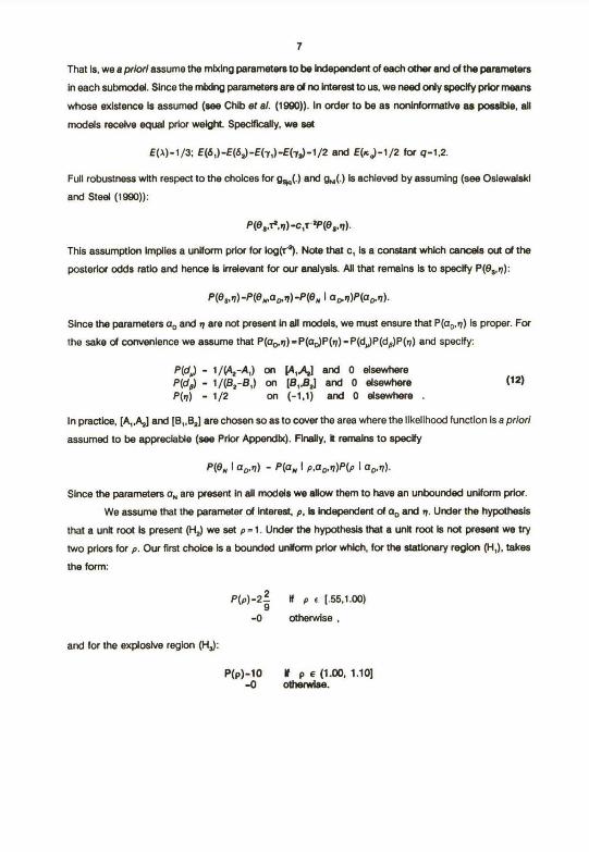
We essume that the parameter d Interest, p, la Independent d ao and q. Under the hypdhesis
that a unft root is present (H~ we set p-1. Urder the hypothesis that a unR root Is not present we try
two priors for p. Our Flrst chok~ Is a bourtded unrtorrn prior wh~h, for the atatlonary repkxt (H,), takes
the form:
P(P)-29 If p e (.55,1.00)
-0 otherwise ,
and for the explosive region (H~:
P(P)-10 N p e(1.00, 1.10]-0 ottterwtse.
8
This type of bounded uniform prkx leads to a truncated Student-t posterlor for p under V, and for p ~ q
under Vx. AltematNely, an Independent Student-t prkx for p wRh Identir.al first two momentsx can be
used to yleld a 2-0 pdy-t posterior density for p(or p ~ 7) (Dreze (1977)). Note that pseudo-random
drawings to be used in the Monte Cado Integration can easUy be made from all these densRies (Richard
and Tompa (19f30)).
Although the first two posterior moments of p may rwt be cruclally aHected by the difference
between priors, Koop er al. (199t ) show that results for n-atep ahead pred~tbn can dt(fer dramatically.'
That Is, predbtNe means and variances wIU exist for any horizon (n) In the case of a bounded unMorm
prior; however the Student prior for p atlows oNy for flnfte predlctNe means (given q) for n up to
approxlmately T, and for finfte predlctive verlancea If n Is less than approximately T~2. In Sectlon 5 we
Introduce a loss functlon based on predlctNe variances whosebefiavior Is expected to dHfer across prbrs
H n Is dose to T~2. t~t course, the tad that moments may not exist will not necessarlly show up dearly
here gNen the inevitable limitatbns of a Monte Carlo analysis whksh uses a finRe number oF repl~atlons.
This concludes our development of aprkx tor the parameters of our sampiing model. It Is worth
emphasizing that, wfth four exceptions, p, q, dM and dp, the priors for all our parameters are
raninformatlve. We believe that the prkxs we aped(y for these exceptlons will not be considered
unreasonable by other researchers.
Section 4: The Posterior Density
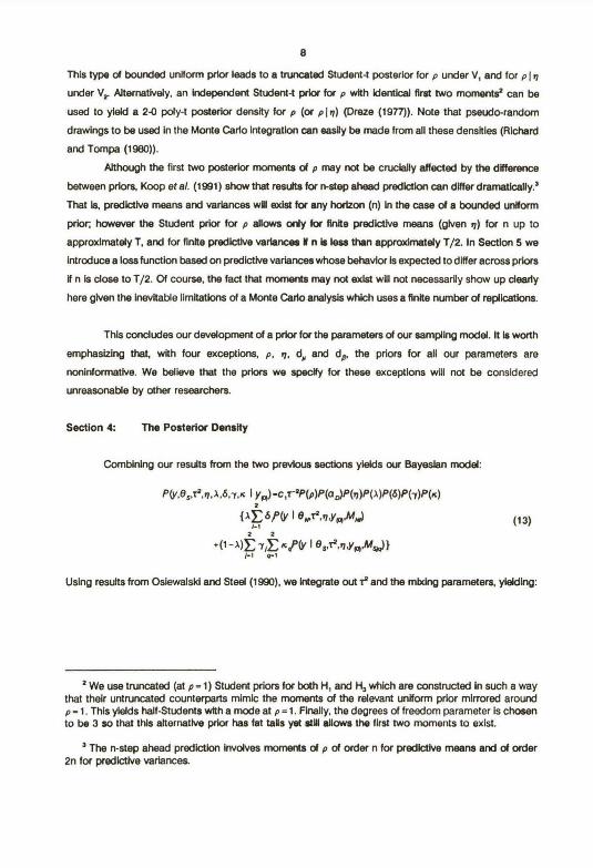
Combining our results from the two prevkxls sectbns ylelds our Bayeslan model:
P(y.9S.~,7,a,ó.7,R I Y~)-c~T-xP(p)P(a~P(7)P(a)P(ó)P(7)P(K)x
{a~óP(v I eMT~.7,Yp,.M'.)~.i
x x
'(t-a)~ 71~K~(yI 8,,~,7J'~,M~}~., o.,
(13)
Using resuKs from Oslewalski and Steel (1990), we kNegrate out tx and the mtxing parameters, yielding:
x We use truncated (at p-1) Student priors for both H, and H, which are constructed In such a waythat their untruncated counterparts mimlc the moments of the relevant uniform prfor mirtored aroundp- t. This ylelds half-Students wfth a mode at p-1. Flnally, the degrees of freedom parameter Is chosento be 3 so that thls alternatlve prkx haa fat taBs yet ~tW ellows the first two moments to exist.
' The n-step ahead prediction Irndves moments of p of order n for pred~tNe means and of order2n for pred~tNe variances.
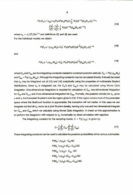
P(Y,95.7 ~ Yp~)-c,P(p)P(ao)P(~){ 3 IY~(7)r'~~Jdw(eM7))-T~2~
3,~ 2~ 2 IV~(o)r'nldsa(es.~)1-'~2}
where c2 z c,I'(T~2)rCT~~ and deflnkbns (5) and (8) ere used.For the IndNidual models we obtaln:
,P(eM~ iY,Yp,M,,,)-CN P(p)P(7)iYi(7~ ~(dw(eM7))-'n
and,
P(es.9 i Y,Ya,My~-Cy;, P(P)P(7)iY~(o)I ~Id~v(Bs,n))-'~: .
(14)
(15)
(18)
where C,~ and C~ are the integrating constants needed to constnrct posterior odds (ie. Cw - P(y ~ yR,M„J
andC~ - P(y ~ y~,M~). Although the integrating constants may be calculated directly, k should be noted
that a„ may be integrated out of (15) and (16) analyt~ally using the properties of mukNariate Student
distributlons. Once a„ is integrated out, the C~,'s and C~'s may be calculated using Monte Car1o
integration. One-d(mensional kttegration Is requlred for calculatlon of C,,,; twotllmensfonal Integration
for C~ and Ce,o; and threeáimenslonal integration for C~. Formally, the posterbr density for ap, given
p and q, is a truncated StudeM-t over the region gNen in (12). If this region covers most of the parameter
space where the likelihood functk~n is appreciable, the truncatkxt will not matter. In this case we can
integrate out the full a9 vector as a Joint Student densky, Ieaving only one and two dimensional integrals
tor Cs,a and C~ which we caiculate using Monte Cario krtegretion. A check on this approximatkxt Is
to pertorm the integration wkh respect to ap numerically by dkect slmulatkxt wkh re)sdkxt.
The IMegrating constant for the sampling model, C- P(y ~ y~), Is given by:
C-s(,L Cwa IL L CyY'
These Integrating constants can be used to calculate the posterior probabAftles ot the various submodels.
P(Mw iY,Y~y)- Cw~6C
P(MN I Y,Y~yI-(CN7tCN7),~
P(M~ I y,y~)- C,~ ~6C
P(My I Y,Yq)-(Cy,~Cy~)~~
P(Msa I Y.Yq)-(Caia`C~~6C.
10The posterkx model probabllRies may Indlcate, among other things, whether structural breaks are present
or H errors exhibR MA(t ) behavlor. ARhough not given here, Inference on the parameters could be obtalned
from weighted averages of (15) and (16) (with a„ posslbly Integrated out), where the welghts are the
relevant model probabllitles.
Under all hypotheses, we use the same general mfxture of submodels for the sampling densiry.
Note, however, that in all cases, the relatNe posterior weights gNen to the submodels depend on the
data.
Sectlon 5: Decision Theory
In the previous sectiona we have described how the posterkx probabAitles of various hypotheses
can be calculated using Bayeslan methods. fiowever, econometricians must frequently make decisions.
For instance, in a pre-testing exercise a decision must hequently be made as to whether a unft root is
present in a series. If present, the series may have to be differenced in a larger VAR model. The Bayeslan
paradigm provides a formal framework for makitig such deciskxts. To make a deciskxt the researcher
specifies a loss function and chooses the actkxt whk:h minimizes expeded loss (see Zellner (1971)). By
focussing on posterior probabYfties, prevbus Bayeslan researchers have impl~itly used a very simple
loss function where all losses attached to Incon-ect decisions are equal. (fhat is, the loss assoclated with
the cholce of a unR root when the series Is statkxtary is equal to that associated with the assumption
of stationarlty when a unit root Is preseM). qassk~l resaerdters use a loas functlon where losses are
asymmetr~, vlz. where the cho~e of a level of slgniflcance Impllcftly deflnes the loss function. Lacking
a measure over the parameter space, dasslcal researchers arv forced to look for, say, dominating
strategies (which are rare) or minimax sdutlons. It Is this lack of fomtal development and justlficatkxi
of a loss functkxt which is, in our opinion, a serlous weakness of previous Bayesian and dassical unit
root studies. This sedion proposes a loss functlon whidt we use to make decisions on whether to accept
or reJect the unR root hypothesis.
Our crfterion for the evaluation of losses associated wfth Incorrect declsions is predictlon. This
criterlon Is ImpoRant because the macroeconom~ tkne serles In this study are frequently used for
prediction (eg. to forecast from VAR models or to calculate impulse responses). The cost oí assuming
stationarity with such models when the serles are reelly ranstatkxtary may be drastically different from
the converse. Since differencea between nonstatkxtary and stationary models are more proraunced for
predfcttve vartances than for predk:tive means, we tiese a loss functk~tt on pred~tNe varlartces. GNen
that the precision of forecasts Is often a crucial Issue we belleve this approach to be a sensible otte.
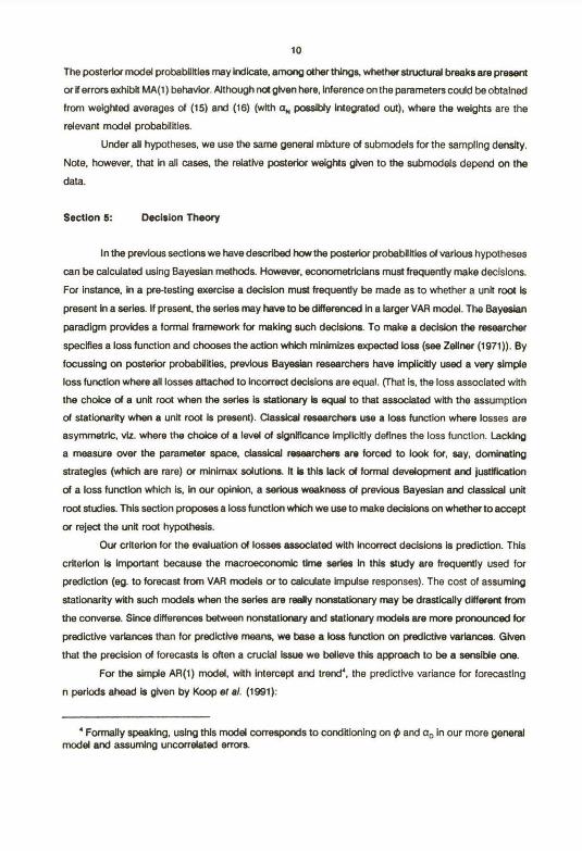
For the simple AR(1) model, with intercept and trerá', the predictive variance for forecasting
n periods ahead Is given by Koop et el. (1991):
' Forrnally speaking, using thls model corresponds to conditloning on ~ and ao In our more generalmodel and assuming uncorrelated errora.
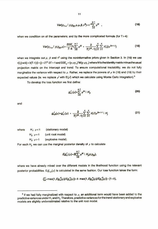
it
n-,
V~RYT.n ~ Y.YRy,P.M.B.t~'~-:F. PL .wo
when we condRion on all the parameters; and by the more complbated fonnuia (for T~4):
~.E n-1 2 n nV~YT.n ~ YYpI.P)-4(~. Py ' ~7q-1)~~ Kf~AP~~~) (19)
when we integrate out N, ~ and r2 using the nonlydomtatNe priors gNen In Sectkxt 3. In (19) we use
r(I,j) ~61jt3(T-1) (i t j) f 2T2-3T t 1 and SSEo s (y-py.,)'M(y-py-,) where M is the Identirymatrix minusthe usual
projection matrix on the intercept and trend. To ensure computational tractability, we do not fully
marginalize the varlance wfth respect to p. Rather, we replace the powers of p In (18) and (19) by thelr
expected values (le. we replace p~ wlth E(p~) which we calculate using Monte Carlo Integratlon).'
To develop the loss functlon we first deflne:
n-1
Dnt(P)'~ PL I HjE.o
and
DnR(P)~8át(P) a ~~-')~~r(~nPSn-F~~ H~
where H,: p ~ 1 (statkxtary model)
Hz: p -1 (unit root model)
H,: p ~ 1 (explosNe model).
For each Hi, we can use the marginal posterlor densky of p to calculate
n-1EDát(P)'QF, D~ I H~YYp~.
Fo
l2~)
where we have already mixed over the different models In the Iikelihood function using the relevant
posterlor probabllftles. Eg',,,,(p) Is calculated In the 9ame fashbn. Our loss tunctlon takea the form:
t'd,-max(~.EDnÁP)IEBn~P))tb ntax(1.Eyn`u(PuEDn.d~P))-(i.b).
' If we had fully marginalized with respect to p, an addRbnal term wouki have been added to thepredlctNe variances under H, and H,. Therefore, predictNevariances forthe trend-stationary and explosfvemodels are slightly underestimated relatfve to the unft root model.
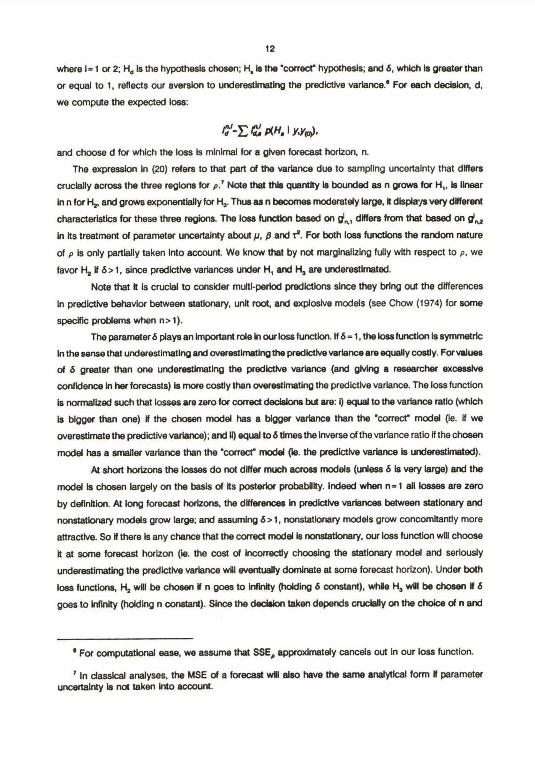
where I~ 1 or 2; H, Is the hypothesis chosen; H~ Is the 'correct' hypdhesis; and d, whid~ is preater than
or equal to 1, reflects our aversion to underestlmatirq the predk;tNe variance.' For each decislon, d,
we compute the expected loss:
~-~ ~~ P(H. I Y.Ypt).
and choose d for which the loss Is m(nlmal for a gNen forecast horizon, n.
The expressbn In (20) refers to that part d the varlance due to sampling uncertainty that differs
cruclally across the three regkxre for p.' Note that tf~ls quar~tlty Is bounded as n prowa for H„ Is Ilnear
In n for Hr and grows exporterttlaily for H,. Thus as n becomea moderately large, It displays very dHterent
characteristics for these three regions. The losa furtation based on q~,~, dNfers from that based on g~„~
in fts treatment of parameter uncertafrny about N, p and r'. For both loas functions the random nature
of p is only partlally taken into account. We know that by not marginalizing fully wfth respect to p, we
favor H, rt ó ~ 1, since predictNe variances under H, and H, are underestlmated.
Note that á is cruclal to conskier muftl-perkxi pred~tions since they bring out the dffferences
In predictNe behavkx between statkxiary, unft root, and explosNe models (see Chow (1974) for some
specific prd~lems when n~ 1).
The parameter d plays an Important rde In our kus function. If d - 1, the k~ss function Is symmetric
In the sense thet underestimatinq and overestimatlnp the predkKNe varlence are equally costly. For values
of d greater than one underestimating the predlctNe variance (and gNing a researcher excesslve
confkience In her forecasts) is more cosUy than overestimating the predictNe varlance. The loss function
is nonnalized such that losses are zero for correct dedsbrw twt are: I) equa! to the varlance ratlo (whlch
is bigger than one) H the chosen model has a bigger varlance than the 'correcC model (le. if we
overestimate the predictive variartce); and ii) equal to d tknes the Inverse d the varfance ratlo if the chosen
model has a smailer varlance than the 'corred' model ( fe. the pred~tNe variance is underestimated).
At short horizons the losses do not differ much acrosa models (urdess d is very large) and the
model b chosen largely on the basis of Rs posterior probabpiry. Indeed when n: t all losses are zero
by deflnftton. At long forecast horizons, the dHferences In predk.tNe variencea between statkxiary ard
nonstatkmary models grow large; and assuminp d ~ 1, nonstatkx~ary models grow concomftanUy more
attractNe. So ff there is any chence that the corred model Is nortstatkxiary, our loss functbn w01 choose
R at some forecast horizon ( le. the cost d Incorrectly choosing the stationary model and seriously
underestimating the predictNe variance wYl ever~tually dominate at some foreqst horizon). Under both
loss fundkxis, H, wBl be chosen M n goes to kdktity (holdirq d constant), wnYe H, wul be dwsert M d
goes to kdinity ( hdding n constant). Sirtce the decislon taken depends cnx~elly on the choice of n and
' For computatkxial aese, we assume that SSE, approximetely cancels out In our loss functfon.
' In dassical analyses, the MSE of a forecaat wll also heve the same anafyt~al form If parameteruncertalnry Is n~ taken Into accour~t.

13
b, we do a senskNfry analysfs over these two parameters.
The decislon theory approach is based on the assumptbn that researchers are Interested In
choosing a particular region for p since they may wlaFt, for Instance, to difference the data. However,
In cases where such a pretest strategy Is not required, we suggest basing predlctlons on a mlxture over
regions for p weighted wkh the relevaM poaterlor probebllkies.
Section 6: Empiricai ResuKs
This sedlon presents evidence on the existence of a unk root in the Nelson-Plosser series. The
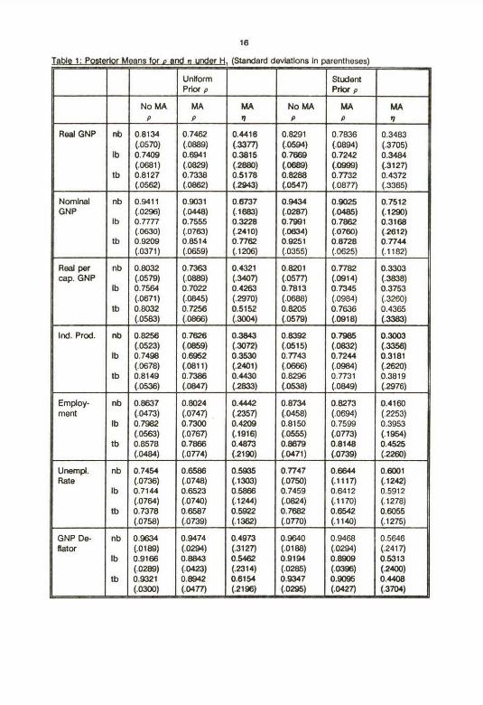
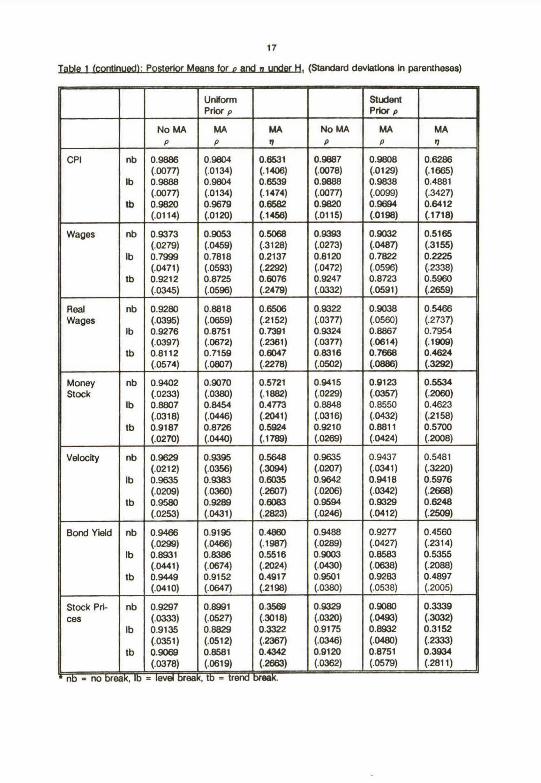
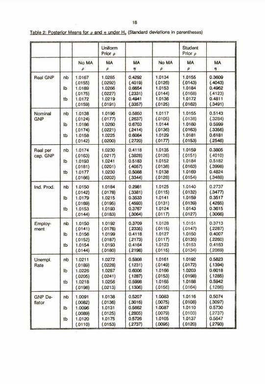
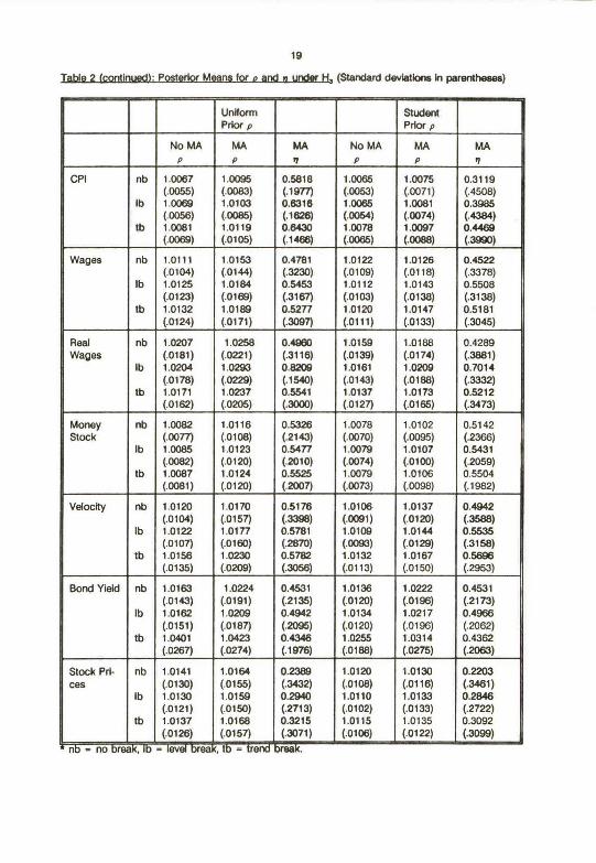
data used are axtended to cover the period untY t9B8 (see Data Appendbc). Tables 1 and 2 present
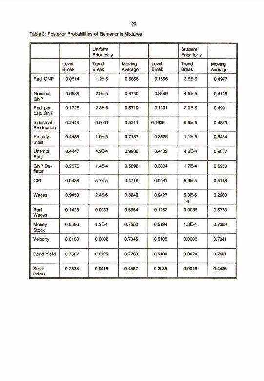
posterior means and standard deviations for p and q under H, and H,, whAe Table 3 presents evidence
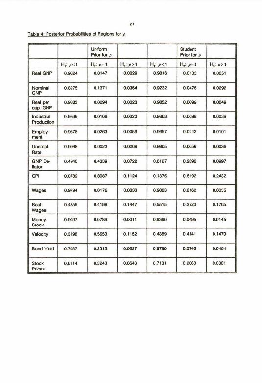
on the presence of structural breaks and moving average errors. Table 4 contalns the posterlor
probabAkles ofH„ H, and H,, and TaWes 5 and 6 aummarize the results of the declslon analysis. Posterkx
odds are calculated for testing the varbus hypotheses wkh respect to p by using the sampling model
weighted over all the submodels. Akhough our primary focus Is on the unk root hypothesis, two subsidiary
questlons are simuitaneously addressed: (1) Is there eviderx:e of one or more structural braaks in our
economlc time series? (2) Is there evidence of MA(i) behavior In the error terms?
Since parameter estimates are only sllghtly relevant to the issues we address in thls paper, we
discuss results onty brieHy. Note Flrst that Tables 1 and 2 support the condusions of Choi (1990): Omkting
the MA(1) component of the error term does Indeed tend to drive estlmates of p towards one In a manner
consistent wkh the asymptot~ bias derNed by Chol. Table 3 contalns the probabAity that an MA(1) error
term Is present as well as the AR(3) component already allowed for In our speciflcatkxi. For many serles
this probabUky is very high and for no series is k small enough to be ignored. Thus Choi's results are
more than Just theoretically Interestfng. The Induskm of a moving average error term wouki appear to
be an important part of any specificatkui. A second polnt worth noting about Tables 1 and 2 Is that
posterior means end standard deviations alone ahouki rat be used to Infer the probability of a hypothesis.
For example, Table 4lndicates that a high probabUky exleta that the real wage series contains a unit root
but the nominal wage does not. This cannot be ascertalned simply by examining the posterior means
and standard deviations in Tables 1 and 2, apdnt whk:h exempirties the hazards of using highest poaterkx
densky intervals for testing purposes.
Wkh respect to structural breaks in Table 3, rate that, aRhough our results are consisterrt wkh
Perron's contentbn that a level break occurred In 19~9 In many macroecorwrnic tlme serles, we find
virtually no evidence for the presence of a trend break In 1973 for any of the series.' As Perron (t989)
notes, models wkh structural breaks tend to yieki less evldence of a unk root.
We do not discuss Table 4 In detaA but we do use the resuks to calculate the expected losses
' Perron Indicates that models wkh a 1973 trend break are mae relevant for post-war quarterly datasets than the long annual data sets used here.

14
requlred for our declslon analysis. For our purposes k b suff~kint to note that resulta show thet trend-
stationarity (H,) Is the most probable hypothesla for most o( the serles (notable exceptkxts are the CPI
and velocity); however, without a fomial loss function k would be rash to rule out the unR root model
at this tlme.
It is worth emphasizing that our loss functlon has two key propertles. First, as long as ó is greater
than one, It Is better to overestlmate than to underestimate predktNe varlances. This property tends to
favor H, over H, and H, over Hz and H,. Indeed as ó goes to Inflnity (holding n constant) H, wlll always
be chosen. Second, there is a tendency In our loss funcclon to favor Hr H, Iies between H, and H, such
that a researcher wAl, loosely speaking, never go too far wrong in dioosing H,. (Poterttial losses would
be very large M, say, H, were ctwsen when H, was the 'corred' model). In fact, as n goes to IMiniry
(hdding ó constant) H2 will always be chosen.' These two propertfes account for most o( the flrdings
In Tables 5 and 6, which present the model chosen for different values of n and ó." Wkh the exception
of the CPI and velocity series and, to a lesser extertt, the GNP deflator and real wage series, H, Is the
model chosen (so long as ó or n is not large). However, dear scope exists for choosing nonstatlonarlty
If underestimating predictNe variances fs feit to be a serbus problem. If ó-100 a researcher would almost
never select the trend-statkxtary modei. There appears to be less sensitNity of our loss function wRh
respect to n. If we restrict attentlon to short- or medium-term forecasts (eg. n ~ 10), only a few cases exlst
where dNferent values of n yleld different conduskxis. A rypk~l example Is real GNP, where, urdess the
researcher Is Interested In forecasting four or more decades Into the future, the trend-statlonary model
Is chosen foró-1 or 10. Only H 6-100 (a strong penatty for underestlmating predictive varlances) Is the
unit root model selected. Overall, we condude that there fs strong evidence In favor of trend-stationarity
for virtually all the series analyzed In thls paper (especlaily as the condftkxiel results gNen In this paper
are blased In favor of Hz); however, as we ehow, researchers with different loss functions may meke
different inferences.
It is krteresting to note that our resufts for ó a 10 correspond dosely to ttase gNen In PhNllps
(1991, repiy) who uses the Phillips-Ploberger posterlor odds test on the same data. The chlet dflference
is that Phillips finds the nominai wage series to contaln a unit root, whereas we only match this finding
if n is very large or ó-100. Note, however, that PhGlips'resuRs are obtalned by using an improper Jeffreys'
prior for p, whereas we use a formal decision theoretic approach based on a strong aversfon to
underestimating predictive variances. Researchera who do not wish to include such an aversion in their
analysis will tend to choose trend-stationarity more often.
` It is worth emphasizing that our fatlure to fully marginallze wfth respect to p favors the unk roothypothesis.
'" Table 5 and 6 correspond to our two loss functions. Because thelr results are very slmllar thefrdifferent treatment of parameter uncertainty in the predictNe variance may not be too important for thepurposes of our analysis for flnfte n. As n goes to ktflrtity these differences may qecome Important (sseKoop et al. ( 1991)).

15
A flnal Issue worth dlscussing Is the senaltNlty oF our results to various priors. Ae descrlbed In
Sectkm 4, we use two differeM priors for p: a haM-Student and a txwnded unHorm prbr. The flrat and
second moments of the halfStudent prior are chosen soas to match the uniform prkx (see footnote 2).
The differences between the two prbrs occur In thkd and hlgher moments. Tables 1 and 2 indk~te that
postedor flrst and second moments do not differ much across the two priors. The remaining tables,
however, Indk;ate somewhet larger dffferences. Thls la eapeclally true of Tables 5 and 6, where In some
cases, the two very similar priors yleld different conduskx~s (eg. Nominai GNP for d s 10 or the GNP
deflator for d~ 1 or 10)." Our decisbn analysls depends upon high order moments of p and our prkxs
dHfer in these high moments. Recall that, whYe all momenta exlet for our bounded uniform prbr, rwne
beyond 2 exlst tor our half-Student prkx. Although Beyesians who use InformetNe priora typk~lly do not
worry about third or higher prkx moments, our anelysis suggests thet care ahould be taken in elk.ltlrp
such prior moments when a decislon analysls whlch krvoNea high order moments Is carrled out. The
effect d prkx moments on the exlstence of predlctNe variances for multi-period forecasting Is formally
analyzed In Koop et al. (1991).
" As described in Section 3, predictNe varlances exlst only for n less than approximately T~2, a factwhlch is Ignored In Tables 5 and 6 where resuRs are occaskmally reported for n~T~2.
16
........ .. . ............ ... ...~.... .... .. ~. ... .. ......... .. ~ ~~.~.....~... ....-.............. t.,........~.......,~
UnMorm StudentPrior p Prior p
No MA MA MA No MA MA MAv v n v a n
Real GNP nb 0.8134 0.7462 0.4418 0.8291 0.7836 0.3483(.0570) (.0889) (.33Tn (.0594) (.0894) (.3705)
Ib 0.7409 0.6941 0.3815 0.7669 0.7242 0.3484(.0681) (.0829) (.2880) (.0689) (.0999) (.3127)
tb 0.8127 0.7338 0.5178 0.8288 0.7732 0.4372(.0562) (.0862) (.2943) (.0547) (.0877) (.3365)
Nominal nb 0.9411 0.9031 0.8737 0.9434 0.9025 0.7512GNP (.0296) (.0448) (.1683) (.0287) (.0485) (.1290)
Ib 0.7777 0.7555 0.3228 0.7991 0.7862 0.3168(.0630) (.0783) (.2410) (.0834) (.0760) (.2612)
tb 0.9209 0.8514 0.7782 0.9251 0.8728 0.7744(.0371) (.0659) (.1206) (.0355) (.0625) (.1182)
Real per nb 0.8032 0.7363 0.4321 0.8201 0.7782 0.3303cap. GNP (.0579) (.0889) (.3407) (.0577) (.0914) (.3838)
Ib 0.7564 0.7022 0.4263 0.7813 0.7345 0.3753(.0671) (.0845) (.2970) (.0688) (.0984) (.3260)
tb 0.8032 0.7256 0.5152 0.8205 0.7636 0.4365(.0583) (.0866) (.3004) (.0579) (.0918) (.3383)
Ind. Prod. nb 0.8256 0.7826 0.3843 0.8392 0.7985 0.3003(.0523) (.0859) (.3072) (.0515) (.0832) (.3356)
Ib 0.7498 0.6952 0.3530 0.7743 0.7244 0.3181(.0678) (.0811) (.2401) (.0666) (.0984) (.2620)
tb 0.8149 0.7386 0.4430 0.8296 0.7731 0.3819(.0536) (.0847) (.2833) (.0538) (.0849) (.2976)
Employ- nb 0.8637 0.8024 0.4442 0.8734 0.8273 0.4160ment (.0473) (.0747) (.2357) (.0458) (.0694) (.2253)
Ib 0.7982 0.7300 0.4209 0.8150 0.7599 0.3953(.0563) (.0767) (.1916) (.0555) (.0773) (.1954)
tb 0.8578 0.7866 0.4873 0.8879 0.8148 0.4525(.0484) (.0774) (.2190) (.0471) (.0739) (.2260)
Unempl. nb 0.7454 0.6586 0.5935 0.7747 0.6644 0.6001Rate (.0736) (.0748) (.1303) (.0750) (.1117) (.1242)
Ib 0.7144 0.6523 0.5866 0.7459 0.6412 0.5912(.0764) (.0740) (.1244) (.0824) (.1170) (.1278)
tb 0.7378 0.6587 0.5922 0.7682 0.6542 0.6055(.0758) (.0739) (.1362) (.0770) (.1140) (.1275)
GNP De- nb 0.9634 0.9474 0.4973 0.9640 0.9468 0.5646flator (.0189) (.0294) (.3127) (.0188) (.0294) (.2417)
Ib 0.9166 0.8843 0.5462 0.9194 0.8909 0.5313(.0289) (.0423) (.2314) (.0285) (.0396) (.2400)
tb 0.9321 0.8942 0.6154 0.9347 0.9095 0.4408(.0300) (.0477) (.2196) (.0295) (.0427) (.3704)
17
T~ble 1(continued): Posterkx Means for n and n under H, (Standard devlatbns In parentheses)
UnHonn StudentPrkx p Prlor p
No MA MA MA No MA MA MAP P 9 P P 7
CPI nb 0.9886 0.9804 0.8531 0.9887 0.9808 0.6286(.oon) (.o13a) (.14a6) (.oo7e) (.o12s) (.1ss5)
Ib 0.9888 0.9804 0.6539 0.9888 0.9838 0.468t(.0077) (.0134) (.1474) (.0077) (.0099) (.3427)
tb 0.9820 0.9679 0.6682 0.9820 0.9694 0.fi412(.0114) (.0120) (.1456) (.0115) (.0198) (.1718)
Wages nb 0.9373 0.9053 0.5068 0.9393 0.9032 0.5165(.0279) (.0459) (.3128) (.0273) (.0487) (.3155)
Ib 0.7999 0.7818 0.2137 0.8120 0.7822 0.2225(.0471) (.0593) (.2292) (.0472) (.0596) (.2338)
tb 0.9212 0.8725 0.6076 0.9247 0.8723 0.5960(.0345) (.0596) (.2479) (.0332) (.0591) (.2659)
Real nb 0.9280 0.8818 0.6506 0.9322 0.9038 0.5466Wages (.0395) (.0659) (.2152) (.0377) (.0560) (.2737)
Ib 0.9276 0.8751 0.7391 0.9324 0.8867 0.7954(.0397) (.0672) (.2381) (.0377) (.0614) (.1909)
tb 0.8112 0.7159 0.6047 0.8316 0.7668 0.4624(.0574) (.0807) (.2278) (.0502) (.0886) (.3292)
Money nb 0.9402 0.9070 0.5721 0.9415 0.9123 0.5534Stock (.0233) (.0380) (.1882) (.0229) (.0357) (.2060)
Ib 0.8807 0.8454 0.4773 0.8848 0.8550 0.4623(.0318) (.0446) (.2041) (.0316) (.0432) (.2158)
tb 0.9187 0.8726 0.5924 0.9210 0.8811 0.5700(.0270) (.0440) (.1789) (.0269) (.0424) (.2008)
Veloclty nb 0.9629 0.9395 0.5648 0.9635 0.9437 0.5481(.0212) (.0356) (.3094) (.0207) (.0341) (.3220)
Ib 0.9635 0.9383 0.6035 0.9642 0.9418 0.5976(.0209) (.0360) (.2607) (.0206) (.0342) (.2668)
tb 0.9580 0.9289 0.6083 0.9594 0.9329 0.6248(.0253) (.0431) (.2823) (.0246) (.0412) (.2509)
Bond Yield nb 0.9466 0.9195 0.4860 0.9488 0.9277 0.4560(.0299) (.0466) (.1987) (.0289) (.0427) (.2314)
Ib 0.8931 0.8386 0.5518 0.9003 0.8583 0.5355(.0441) (.0674) (.2024) (.0430) (.0638) (.2088)
[b 0.9449 0.9152 0.4917 0.9501 0.9283 0.4897(.0410) (.0647) (.2198) (.0380) (.0538) (.2005)
Stock Pri- nb 0.9297 0.8991 0.3569 0.9329 0.9080 0.3339ces (.0333) (.0527) (.3018) (.0320) (.0493) (.3032)
Ib 0.9135 0.8829 0.3322 0.9175 0.8932 0.3152(.0351) (.0512) (.2367~ (.0346) (.0480) (.2333)
tb 0.9069 0.8581 0.4342 0.9120 0.8751 0.3934(.0378) (.0619) (.2663) (.0362) (.0579) (.2811)
n z no rea , - ev rea , t - re ea .
18
Table 2: Posterior Means for a and n under H, (Standard devlations in parentheses)
Un'rform StudentPrior p Prior p
No MA MA MA No MA MA MAP P 9 P P 9
Real GNP nb 1.0167 1.0285 0.429Q 1.0134 1.0155 0.3609(.0155) (.0292) (.4019) (.0126) (.0143) (.4043)
Ib 1.0189 1.0266 0.6854 1.0153 1.0184 0.4962(.0175) (.0227) (.2331) (.0144) (.0168) (.4123)
tb 1.0172 1.0219 0.4la41 1.0136 1.0172 0.4811(.0159) (.0191) (.3357) (.0125) (.0162) (.3491)
Nominal nb 1.0138 1.0196 0.5850 1.0117 1.0155 0.5143GNP (.0124) (.0177) (.2637) (.0105) (.0138) (.3284)
Ib 1.0186 1.0260 0.6703 1.0144 1.0180 0.5999(.0174) (.0221) (.2414) (.0136) (.0183) (.3356)
tb 1.0158 1.0225 0.6064 1.0129 1.0181 0.6181(.0142) (.0200) (.2720) (.0177) (.0153) (.2546)
Real per nb 1.0174 1.0230 0.4118 1.0135 1.0159 0.3805cap. GNP (.0163) (.0217) (.3828) (.0126) (.0151) (.4010)
Ib 1.0193 1.0241 0.5183 1.0152 1.0184 0.5182(.0181) (.0201) (.4057) (.0138) (.0163) (.3998)
tb 1.0177 1.0230 0.5088 1.0138 1.0169 0.4824(.0166) (.0202) (.3344) (.0128) (.0154) (.3488)
Ind. Prod. nb 1.0150 1.0184 0.2981 1.0125 1.0140 0.2737(.0142) (.0178) (.3381) (.0115) (.0132) (.3477)
Ib 1.0179 1.0215 0.3533 1.0141 1.0159 0.3517(.0169) (.0195) (.4593) (.0131) (.0139) (.4285)
tb 1.0153 1.0193 0.3767 1.0124 1.0143 0.3615(.0144) (.0183i (.3064) (.0117) (.0127) (.3066)
Employ- nb 1.0150 1.0192 0.3709 1.0128 1.0151 0.3713ment (.0141) (.0176) (.2335) (.0115) (.0147) (.2287)
Ib 1.0156 1.0199 0.4118 1.0127 1.0150 0.4007
(.0152) (.0187) (.2173) (.0117) (.0135) (.2260)tb 1.0154 1.0193 0.4164 1.0123 1.0153 0.4163
(.0144) (.O1B0) (.2198) (.0115) (.0134) (.2069)
Unempl. nb 1.0211 1.0272 0.5908 1.0161 1.0192 0.5823Rate (.0189) (.0228) (.1231) (.0149) (.0172) (.1394)
Ib 1.0226 1.0287 0.6006 1.0166 1.0203 0.6018(.0205) (.0241) (.1287) (.0153) (.0198) (.1285)
tb 1.0218 1.0256 0.5998 1.0165 1.0188 0.5942(.0198) (.0213) (.1306) (.0156) (.0164) (.1286)
GNP De- nb 1.0091 1.0138 0.5207 1.0083 1.0116 0.5074flator (.0082) (.0136) (.3016) (.0075) (.0108) (.3097)
Ib 1.0096 1.0131 0.5662 1.0087 1.0110 0.5730(.OOli9) (.0125) (.2805) (.0079) (.0103) (.2737)
tb 1.0120 1.0175 0.5726 1.0105 1.0137 0.5647(.Ot 10) (.0153) (.2737) (.0095) (.0120) (.2793)
19
Table 2(contlnued): Posterior Means for n and n under H, (Standard devlatkxis in parerrtheses)
Unfform StudentPrior p Prior p
No MA MA MA No MA MA MAv v n v v n
CPI nb 1.0087 1.0095 0.5818 1.0065 1.0075 0.3119(.0055) (.0083) (.1977) (.0053) (.0071) (.4508)
Ib 1.0069 1.0103 0.6316 1.0065 1.0081 0.3985(.0056) (.0085) (.1626) (.0054) (.0074) (.4384)
tb 1.008t 1.0119 0.8430 1.0078 1.0097 0.4469(.0069) (.0105) (.1466) (.0065) (.0088) (.3990)
Wages nb 1.0111 1.0153 0.4781 1.0122 1.0126 0.4522(.0104) (.0144) (.3230) (.0109) (.0118) (.3378)
Ib 1.0125 1.0184 0.5453 1.0112 1.0143 0.5508(.0123) (.0169) (.3167) (.0103) (.0138) (.3138)
tb 1.0132 1.0189 0.5277 1.0120 1.0147 0.5181(.0124) (.0171) (.3097) (.0111) (.0133) (.3045)
Real nb 1.0207 1.0258 0.4960 1.0159 1.0188 0.4289Wages (.0181) (.0221) (.3116) (.0139) (.0174) (.3881)
Ib 1.0204 1.0293 0.8208 1.0161 1.0209 0.7014(.0178) (.0229) (.1540) (.0143) (.0188) (.3332)
tb 1.0171 1.0237 0.5541 1.0137 1.0173 0.5212(.0162) (.0205) (.3000) (.0127) (.0165) (.3473)
Money nb 1.0082 1.0116 0.5326 1.0078 1.0102 0.5142Stock (.0077) (.0108) (.2143) (.0070) (.0095) (.2366)
Ib 1.0085 1.0123 0.5477 1.0079 1.0107 0.5431(.0082) (.0120) (.2010) (.0074) (.0100) (.2059)
tb 1.0087 1.0124 0.5525 1.0079 1.0106 0.5504(.0081) (.0120) (.2007) (.0073) (.0098) (.1982)
Velocfty nb 1.0120 1.0170 0.5176 1.0106 1.0137 0.4942(.0104) (.0157) (.3398) (.0091) (.0120) (.3588)
Ib 1.0122 1.0177 0.5781 1.0109 1.0144 0.5535(.0107) (.0160) (.2870) (.0093) (.0129) (.3158)
tb 1.0156 1.0230 0.5782 1.0132 1.0167 0.5696(.0135) (.0209) (.3058) (.0113) (.0150) (.2953)
Bond Yield nb 1.0163 1.0224 0.4531 1.0136 1.0222 0.4531(.0143) (.0191) (.2135) (.0120) (.0196) (.2173)
Ib 1.0162 1.0209 0.4942 1.0134 1.0217 0.4966(.0151) (.0187) (.2095) (.0120) (.0196) (.2062)
tb 1.0401 1.0423 0.4346 1.0255 1.0314 0.4362(.0267) (.0274) (.1976) (.0188) (.0275) (.2063)
Stock Pri- nb 1.0141 1.0164 0.2389 1.0120 1.0130 0.2203ces (.0130) (.0155) (.3432) (.0108) (.0116) (.3461)
Ib 1.0130 1.0159 0.2940 1.Oi10 1.0133 0.2846(.0121) (.0150) (.2713) (.0102) (.0133) (.2722)
tb 1.0137 1.0168 0.3215 1.0115 1.0135 0.3092(.0126) (.0157) (.3071) (.O t p6) (.0122) (.3099)
nb - no break, Ib - level break, tb - trenci breek.
20Table 3: Posterior Probabilities of Elements In Mixtures
Unlform StudentPrkx for p Prlor for p
l.evel Trend Movkq Level Trend MovkigBreak Break Average Break Break Average
Real GNP 0.0614 1.2E-5 0.5856 0.1556 3.6E~ 0.4977
Nominai 0.6639 2.9E-5 0.4740 0.8489 4.5E-5 0.4146GNPReal per 0.1728 2.3E-5 0.5719 0.1391 2.0E-5 0.4991cap. GNP
Industrlal 0.2449 0.0001 0.5211 0.1tí~l.ó 9.8E-5 0.4829Production
Employ- 0.4488 1.0E-5 0.7137 0.3626 1.1E-5 0.6454ment
Unempl. 0.4447 4.9E~ 0.9930 0.4102 4.8E-4 0.9857Rate
GNP De- 0.2676 1.4E-4 0.5892 0.3034 1.7E-4 0.5950eatorCPI 0.0438 5.7E~i 0.4718 0.0461 5.9E-5 0.5148
Wages 0.9453 2.4Eó 0.3240 0.9427 5.3E~.~
0.2960
Real 0.1428 O.IX)33 0.5554 0.1252 0.0085 0.5773Wages
Money 0.5586 1.2E-4 0.7550 0.5194 1.3E-4 0.7399Stock
Veloclty 0.01t)8 0.0002 0.7345 0.0108 0.0002 0.7341
Bond Yieid 0.7527 0.0125 0.7763 0.9180 0.0070 0.7661
Stock 0.2838 0.0018 0.4587 0.2935 0.0018 0.4485Pr~es
21
Table 4: Posterlor Probabilitles oi Realons for n
UnHormPrkx for p
StudentPrkx for p
H,: p~1 Hz: p-1 H~: p~t H,: p~1 H:: p-1 H~: p~1
Real GNP 0.9824 0.0147 0.0029 0.9816 0.0133 0.0051
NominaiGNP
0.8275 0.1371 0.0354 0.9232 0.0476 0.0292
Real percap. GNP
0.9883 0.0094 0.0023 0.9852 0.0099 0.0049
IndustrialProduction
0.9869 0.0108 0.0023 0.9863 0.0099 0.0039
Employ-ment
0.9678 0.0263 0.0059 0.9657 0.0242 0.0101
Unempl.Rate
0.9968 0.0023 0.0009 0.9905 0.0059 0.0036
GNP De-flator
0.4940 0.4339 0.0722 0.6107 0.2896 0.0997
CPI 0.0789 0.8087 0.1124 0.1376 0.6192 0.2432
Wages 0.9794 0.0176 0.0030 0.9803 0.0162 0.0035
RealWages
0.4355 0.4198 0.1447 0.5515 0.2720 0.1765
MoneyStock
0.9097 0.0789 0.0011 0.9360 0.0495 0.0145
Velocity 0.3198 0.5650 0.1152 0.4389 0.4141 0.1470
Bond Yleld 0.7057 0.2315 0.0627 0.8790 0.0746 0.0464
StockPrbes
0.6114 0.3243 0.0643 0.7131 0.2068 0.0801
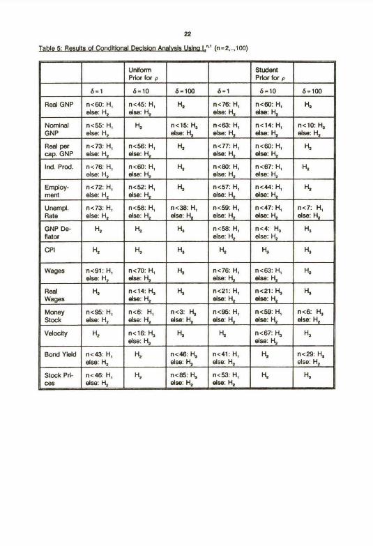
zzTable 5: Results of Conditional Decis(on Analvsis Usinq,Ja"~' (n-2,..,100)
Unlform StudentPrkx for p Prkx for p
b-1 ó-10 ó-100 d-1 b310 á-100
Real GNP nc60: H, nc45: H, Hz nc76: H, nc60: H, Hzelse: H2 else: Hz else: Hz elae: H2
Nominal n~55: H, Hz nc15: H, nc63: H, n~14: H, nc10: H,GNP eise: H2 else: H, else: H, else: Hz else: Hz
Real per nc73: H, nc56: H, Hz nc77: H, nc60: H, Hzcap. GNP else: HZ else: Hz else: H, else: FLr
Ind. Prod. nc76: H, nc60: H, Hy nc80: H, nc87: H, H,else: H, else: H, else: Hz else: Hz
Employ- nc72: H, nc52: H, H, nc57: H, nc44: H, Hpment else: Hz else: Hz else: Hz else: H,
Unempl. n~73: H, nc58: H, nc36: H, n~59: H, nc47: H, n~7: H,Rate else: Hz else: H2 else: H7 else: H2 else: H, slse: Hz
GNP De- H~ Hz H, nc58: H, nc4: H, H,flator else: Hz else: H2
CPI H, H, H, H, H, H,
Wages nc91: H, nc70: H, Fiz nc76: H, nc63: H, H,slse: Hz else: H, slse: H, else: H,
Real Hz nc14: H, H, nc21: H, nc21: H, H,Wages else: H2 else: Hz else: Hz
Money nc95: H, nc6: H, nc3: H, nc95: H, nc59: H, ncó: H,Stock else: HZ else: H, else: HII else: Hz else: Hz else: H,
Velocity Hz nc16: H, H, H, nc67: H, H,else: Hz else: HZ
Bond Yleld n~43: H, Hz nc48: H, nc41: H, H, nc29: H,else: Hz else: H, else: Hz else: Hz
StoCk Pri- n~46: H, Hz nct35: H, nc53: H, H, H,ces else: Hz else: H2 else: H,

23
TaWe 6: ResuRs of Decision Analvsis Usina I.~ ( n~2,..,t00)
Unfform StudentPrkx for p Prkx for p
ó-1 ó-t0 óz100 ó ~1 ó-10 ó~100
Real GNP nc67: H, nc49: H, Hz nc83: H, nc67: H, Hzslse: H2 else: Hz else: H2 else: H2
Nominal nc62: H, Hz nc13: H, nc70: H, nc25: H, nc10: H,GNP else: Hz else: Hz else: H, else: Hz else: H,
Real per nc81: H, nc62: H, H~ nc85: H, nc67: H, Hzcap. GNP else: Hz else: H, else: H, else: Hz
Ind. Prod. nc82: H, n~65: H, Hi nc85: H, nc72: H, H2else: Hz else: HZ else: H, 91se: Hz
Employ- nc80: H, nc57: H, H, nc68: H, nc56: H, nc7: H,ment else: H2 else: Hz else: Hz else: H2 slse: Hz
Unempl. nc60: H, nc63: H, nc41: H, nc62: H, nc49: H, HzRate else: Hz else: HZ else: Hz else: Hz else: H2
GNP De- HZ H, H, nc64: H, nc4: H, H,flator else: H, else: HZ
CPI Hs H, H, Hp H, H,
Wages H, nc78: H, Ht nc83: H, n~69: H, Hzelse: H, else: Hs else: Hz
Real Hz n~13: H, H, nc16: H, nc20: H, H,Wages else: H, else: Hz else: Hz
Money H, ncó: H, nc3: H, H, nc65: H, nc5: H,Stock else: HZ else: Hz else: H, else: H2
Velocity Hz n c 15: H, H, Hz n c 26: H, H,else: H, else: HZ
Bond Yield nc47: H, Hz nc33: H, nc44: H, H, nc23: H,else: HZ else: Hz else: Hz else: HZ
Stock Pri- n~50: H, H, nc58: H, nc56: H, HQ nc71: H,ces el,e H., else: Hz else: H, 61se: H~

2a
Section 7: Conclusions
The paper develops a fomial declsion theoretic approach to testing for unit roots which InvoNes
the use of a loss function based on pred~tNe var~rx~e. It also etdends the dass d Iikellhood functbns
In the Bayeslan unit root Ifterature by using a IIkelRaoci function wh~h isa mb4ure over submodels whk:h
dfffer in covarlance structure and in the treatment of structural breaks. Each of the IndNidual Iikelihoods
mixed into the overall likellhood functkm belongs to the dass of general elllptk~l densRles.
Our empirical results indirate that a hlgh posterfor probabtlity of trend-statlonarRy exists for most
of the econom~ time series. However, N there Is a high coat to underestlmating predictNe varlances, our
decision analysis indicates that trend-stationarity Is not necessar9y the preferred cholce.

zsData Appendix
The data used In this paper are that of Neison and Plosser (1982) updated to 1988 by Herman vanDijk. Primary data sources are listed in Schotman and van Dljk (1991 b). All data are annual U.S. dataWe take natural lops of all series except for the bond yield. The fourteen series are:
1) Real GNP (1909-1988).2) Nominal GNP (1909-1988).3) Real per capne GNP (1909-1988).4) Industrlal productlon (1860-1988).5) Employment (1890-1988).6) Unemployment rate (1890-1988).7) GNP d~lator (1889-1988).8) Consumer Price Index (1860-1988).9) Nominal wages (1900-1988).10) Real waqes (1900-1988).11) Money stock (1889-1988).1z) velocny (18ss-teea).13) Bond yield (1900-1988).14) Common siock prices (1871-1988).
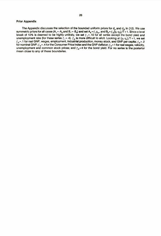
2sPrior Appendix
The Appendix discusses the selection of the bounded uniform prlors for d and dp In (12). We usesymmetric prkxs for all cases (A, a-A, and B, s-Bz) ard set A,- S,yr, and B,.SIICyTy~~T t 1. Since a levelbreak d 1096 Is deemed to be hlghly unlikely, we set S,-.10 for all serles except the bond yleld andunemploymerrt rate (for these serles ~, -.4~. ip Is more dNFlcuit to ellcit. Looking at (yTy~~T t t, we setSzs.t for real GNP, wages, employment, Industrlal productkxi, money stock, and GNP per capita; S,z.2for rwminal GNP; f,-.4 for the Gonsumer Pr~e Index end the GNP deflator; S,-1 for real wages, veloclty,unemployment and common stock prk.es; end S~-4 tor the txxid yleld. For no serles Is the posterkxmean close to any of these boundarles.
27
References
Baillie, R. (1979). 'The Asymptotic Mean Squared Error d Multistep Prediction from the Regression Modelwfth AutoregressNe Enors', Journal oi the Amerlcan StatlsUcal ASSOCIaUon, 74, 175-184.
Baner)ee, A., Lumsdaine, R. and Stock, J. (1990). 'RecursNe and Sequentlal Tests d the Unft Root andTrend Break Hypotheses: Theory and Intematkxiel Evklence', NBER Working Paper No. 3510.
Chib, S., Osiewalski, J. and Steel, M. (1990). 'Regresslon Models Under CompeUrq Covarlance Matrlces:A Bayeslan PerspectNe', CentER Discusslon Paper No. 9063, Tllburg Universtty.
Choi, I. (1990). 'Most U.S. Economic Tlme Series Do Not Have UnR Roots: Nelson and Plosser's (1982)Resufts Reconsfdered', manuscript.
Chow, G. (1974). 'Multiperlod Predictions from Stochastlc Dlfference Equations by Bayesian Methods',In Studles In BayesJan EconometrJcs end StaUstlcs, eda. S. Fienberg and A. Zeliner, Amsterdam: North-Holland, chapter 8.
DeJong, D. and Whiteman, C. (1991a). ~rends and Random Walks in Macro-economic Time Serles: AReconskieration Based on the Ukelihood Principle', forthcoming, Joumal of Monetary Economlcs.
DeJong, D. and Whiteman, C. (1991 b). ~he Temporal StabAlry ot DNkiends and Stock Prices: Evfdencefrom the LJkelihood Functton', American Economlc ReNew, 81, 600.617.
Dickey, D. and Fuller, F. (1979). 'Distributlon of the Estimators for AutoregressNe Time Series wfth a UnRRooC, Journal ot the Amerlcan Statlstlcal AssoclaUon, 74, 427-031.
Dreze. J. (1977). 'Bayeslan Regression Analysls Using Pdy-t DensRles', Joumal ol Econometrlcs, e, 329-354.
Koop, G. (1991a). "Objective' 8ayesian Unft Root Tests', torthcoming, Journal otApplfed Econometrks.
Koop, G. (1991 b). 'Intertemporal Properties of Real Output: A Bayesian Approach', Joumel oi Businessand Economlc Statlstlcs, 9, 253-265.
Koop, G., Osiewalski, J. and Steel, M. (1991). 'Bayeslan l.ong Run Pred~tkxi In Time Serles Models',manuscript.
Koop, G. and Steel, M. (1991). 'A Comment on: To CHticize the Critics: An ObjectNe Bayesian Analysisof Stochastic Trends by Peter C. B. PhAlips', forthcoming, Joumal dApplied Econometrlcs.
Nelson, C. and Ptosser, C. (1982). ~rends and Random Walks In Macroeconomlc Time Serles: SomeEviderx,e and Implications', Journal ol Monetary Ecorromks, 10, 139-1G2.
Osiewalskl, J. and Steel, M. (1990). 'Robust Bayeslan Inference In Elliptical Regressbn Models', CeritERDiscussion Paper No. 9032,TAburg UnNersity.
Perron, P. (19t39). ~he Great Crash, the 06 Price Shodc, and the UnR Root Hypotheslá , Econometrlca,57, 136t-t402.
Phillips, P. (1991). ~o Crrtlcize the Critics: An ObjectNe Bayesian Analysls d Stochastic Trendá,forthcoming, Joumsl o! Applled Econometrlcs.
Rlchard, J. and Tompa, H. (1980). 'On the Evaluation of Pdy-t Densfty Functions', Journal oiEconometrlcs, 12, 335-35t.
28
Schotman, P. and van Dijk, H. (t991a). 'A Bayeslan Anelysis of the UnR Roa In Real Exchange Rates',Joumal ol Economevlcs, 49, 195-238.
Schotman, P. and van DI(k, H. (1991b). 'On Bayeslan Routes to Uni[ Roots', Journal ol AppliedEconometrlcs, forthcoming.
Schwert, W. (1987). 'Effects of Model Speclflcation on Tests for UnR Roots in Macroeconomic Data',Joumal ol Monetary Economfcs, 20, 75-103.
Sims, C. (1988). 'Bayesian Skepticism on UnR Root Econornetrk;s', Joumal dEconomlc Dynamlcs andConvd, 12, 463.47a.
Wago, H. arxl Tsuruml, H. (1990). 'A Bayesian Arrelysis of Statkxiarity and the UnR Root Hypothesls',presented at the 6th World Congress of the Econort~r~ Soclety.
Zellner, A. (1971). An Invoductlon to 8ayeslan 1Merence !n Ecorwmetrfcs (John WAey, New York).
ZNOt, E. and PhAllps,P .( 1990). 'A Bayesian Analysls of Trend Determinatkx~ In Economic Time Serles',manuscrlpt.
Discussion Paper Series, CentER, Tilburg Uníversity, The Netherlands:
(For previous papers please
No. Author(s)
9036 J. Driffill
9037 F, van der Ploeg
9G38 A. Robson
9G39 A. Robson
904o M.R. Baye, G. Tianand J. Zhou
9041 M. Burnovsky andI. Zang
9G42 P.J. Deschamps
consult previous discussion papers.)
Title
The Term Structure of Interest Rates:Structural Stability and Macroeconomic PolicyChanges in the UK
9G43 S. Chib, J. Osiewalskiand M. Steel
9G44 H.A. Keuzenkamp
9045 I.M. Bomze andE.E.C. van Damme
9046 E. van Damme
9047 J. Driffill
9G48 A.J.J. Talman
9G49 H.A. Keuzenkamp andF. van der Ploeg
905o C. Dang endA.J.J. Talman
9051 M. Baye, D. Kovenockand C. de Vries
9052 H. Carlsson andE. van Damme
Budgetary Aspects of Economic and MonetaryIntegration in Europe
Existence of Nash Equilibrium in MixedStrategies for Games where Payoffs Need notBe Continuous in Pure Strategies
An "Informationally Robust Equilibrium" forTwo-Person Nonzero-Sum Games
The Existence of Pure-Strategy NashEquilibrium in Games with Payoffs that arenot Quasiconcave
"Costless" Indirect Regulation of Monopolieswith Substantial Entry Cost
Joint Tests for Regularity andAutocorrelation in Allocation Systems
Posterior Inference on the Degrees of FreedomParameter in Multivariate-t Regression Models
The Probability Approach in Economic Method-ology: On the Relation between Haavelmo's
Legacy and the Methodology of Economics
A Dynamical Characterization of Evolution-arily Stable States
On Dominance Solvable Games and EquilibriumSelection Theories
Changes in Regime and the Term Structure:A Note
General Equilibrium Programming
Saving, Investment, Government Finance andthe Current Account: The Dutch Experience
The D-Triangulation in Simplicial VariableDimension Algorithms on the Unit Simplex forComputing Fixed Points
The All-Pay Auction with Complete Information
Global Games and Equilibrium Selection

No. Author(s)
9053 M. Baye andD. Kovenock
9G54 Th. van de Klundert
9055 P. Kooreman
9056 R. Bartels endD.G. Fiebig
905~ M.R. Veall andK.F. Zimmermann
9058 R. Bartels andD.G. Fiebig
9059 F. van der Ploeg
9060 H. Bester
9061 F. van der Ploeg
9062 E. Bennett andE. ven Damme
9063 S. Chib, J. Usiewalskiand M. Steel
9G64 M. Verbeek andTh. Nijman
9065 F, van der Ploegand A. de Zeeuw
9066 F.C. Drost andTh. E. Nijman
9G67 Y. Dai and D. Talman
9068 Th. Nijman andR. Beetsma
9069 F. van der Ploeg
90~0 E. van Damme
9071 J. Eichberger,H. Haller and F. Milne
Title
How to Sell a Pickup Truck: "Beat-or-Pay"Advertisements as Facilitating Devices
The Ultímate Consequences of the New CrowthTheory; An Introduction to the Views of M.Fitzgerald Scott
Nonparemetric Bounds on the RegressionCoefficients when an Explanatory Variable isCategorized
Integrating Direct Metering and ConditionalDemand Analysis for Estimating End-Use Loads
Evaluating Pseudo-RZ's for Binary ProbitModels
More on the Grouped HeteroskedasticityModel
Chennels of International Policy Transmission
The Role of Collateral in a Model of DebtRenegotiation
Macroeconomic Policy Coordination during theVarious Phases of Economic and MonetaryIntegration in Europe
Demand Commitment Bargaining: - The Case ofApex Games
Regression Models under Competing CovarianceMatrices: A Bayesian Perspective
Cen Cohort Data Be Treated as Genuine PanelData?
International Aspects of Pollution Control
Temporal Aggregation of GARCH Processes
Linear Stationary Point Problems on UnboundedPolyhedra
Empirical Tests of a Simple Pricing Model forSugar Futures
Short-Sighted Politicians and Erosion ofGovernment AssetsFair Division under Asymmetric Information
Naive Bayesien Learning in 2 x 2 MatrixGames

No. Author(s)
9072 G. Alogoskoufis endF. van der Ploeg
9G73 K.C. Fung
9101 A. van Soest9102 A. Barten and
M. McAleer
9103 A. Weber
91G4 G. Alogoskoufis andF. van der Ploeg
9105 R.M.W.J. Beetsma
91G6 C.N. Teulings
9107 E. van Damme
9108 E. van Damme
91G9 G. Alogoskoufis andF. van der Ploeg
9110 L. Samuelson
9111 F. van der Ploeg andTh. van de Klundert
9112 Th. Nijman, F. Palmand C. Wolff
9113 H. Bester
9114 R.P. Gilles, G. Owenend R, van den Brink
9115 F. van der Ploeg
9116 N. Rankin
9117 E. Bomhoff
9118 E. Bomhoff
Title
Endogenous Growth end Overlapping Generations
Strategic Industrial Policy for Cournot andBertrand Oligopoly: Management-LaborCooperation as a Possible Solution to theMarket Structure Dilemma
Minimum Wages, Earnings and Employment
Comparing the Empirical Performance ofAlternative Demend Systema
EMS Credibility
Debts, Deficits and Growth in InterdependentEconomies
Bands and Statistical Properties of EMSExchange Rates
The Dlverging Effects of the Business Cycleon the Expected Duration of Job Search
Refinements of Neah Equilibrium
Equilibrium Selection in 2 x 2 Games
Money and Growth Revisited
Dominated Strategies end Commom Knowledge
Political Trade-off between Growth andGovernment Consumption
Premia in Forward Foreign Exchange asUnobserved Components
Bargaining vs. Price Competition in a Marketwith Quality Uncertainty
Games with Permission Structures: TheConjunctive Approach
Unanticipated Inflation and GovernmentFinance: The Case for an Independent CommonCentral Bank
Exchange Rate Risk and Imperfect CapitalMobility in an Optimising Model
Currency Convertibility: When and How? AContribution to the Bulgarian Debate!
Stability of Velocity in the G-7 Countries: AKalman Filter Approach

No. Author(s)
9119 J. Osiewalski andM. Steel
9120 S. Bhattacharya,J. Glazer andD. Sappington
9121 J.W. Friedman andL. Samuelson
9122 S. Chib, J. Osiewalskiand M. Steel
9123 Th. van de Klundertand L. Meijdam
9124 S. Bhattacharya
9125 J. Thomas
9126 J. Thomasend T. Worrall
9127 T. Gao, A.J.J. Talmanand Z. Wang
9128 S. Altug andR.A. Miller
9129 H. Keuzenkamp andA.P. Barten
Title
Bayesian Marginal Equivalence of EllipticalRegression Models
Licensing and the Shering of Knowledge inResearch Joint Ventures
An Extension of the "Folk Theorem" withContinuous Reaction Functions
A Bayesian Note on Competing CorrelationStructures in the Dynamic Linear RegressionModelEndogenous Growth and Income Distribution
Banking Theory: The Main Ideas
Non-Computable Rational ExpectationsEquilibris
Foreign Direct Investment and the Risk ofExpropriation
Modification of the Kojima-Nishino-ArimaAlgorithm and its Computational Complexity
Human Capital, Aggregate Shocks and PanelData Estimation
Rejection without Falsification - On theHistory of Testing the Homogeneity Cunditionin the Theory of Consumer Demand
913G G. Mailath, L. Samuelson Extensive Form Reasoning in Normal Form Gamesand J. Swinkels
9131 K. Binmore andL. Semuelson
Evolutionary Stability in Repeated GamesPlayed by Finite Automata
9132 L. Samuelson andJ. Zhang
9133 J. Greenberg andS. Weber
9134 F. de Jong andF. van der Ploeg
9135 E. Bomhoff
9136 H. Bester andE. Petrakis
Evolutionary Stability in Asymmetric Games
Stable Coalition Structures with Uni-dimensional Set of Alternatives
Seigniorage, Taxes, Government Debt endthe EMS
Between Price Reform and Privatization -Eastern Europe ín Transition
The Incentives for Cost Reduction in aDifferentiated Industry
No. Author(s)
913~ L. Mirman, L. Samuelsonand E. Schlee
9138 c. Dang
9139 A. de Zeeuw
9140 B. Lockwood
9141 C. Fershtman andA. de Zeeuw
914z J.D. Angrist andG.W. Imbens
9143 A.K. Bera and A. Ullah
9144 B. Melenberg andA. van Soest
9145 C. Imbens andT. Lancaster
9146 Th. van de Klundertand S. Smulders
9147 J. Greenberg
9148 S. van Wijnbergen
9149 S. van Wijnbergen
915G G. Koop endM.F.J. Steel
Title
Strategic Information Manipulation inDuopolies
The D2-Triengulation for ContinuousDeformation Algorithms to Compute Solutionsof Nonlinear Equations
Comment on "Nash and Stackelberg Solutions ina Differential Game Model of Capitalism"
Border Controls and Tax Competition in aCustoms Union
Capital Accumulation and Entry Deterrence: AClarifying Note
Sources of Identifying Informatíon inEvaluation Models
Rao's Score Test in Econometrics
Parametric and Semi-Parametric Modelling ofVacation Expenditures
Efficient Estimation and Stratified Sampling
Reconstructing Growth Theory: A Survey
On the Sensitivity of Von Neuman andMorgenstern Abstract Stable Sets: The Stableand the Individual Stable Bargainin~ Set
Trade Reform, Policy Uncertainty and theCurrent Account: A Non-Expected UtilityApproach
Intertemporal Speculation, Shortages end thePolitical Economy of Price Reform
A Decision Theoretic Analysis of the UnitRoot Hypothesis Using Mixtures of EllipticalModels

P~ R~x 9rn~~ ~~n~ I F TII BURG. THE NETHERLAND;Bibliotheek K. U. Brabantuiiwia~aN i~M imw i~ u~ i u