TIG WELDING SKILL EXTRACTION

USING A MACHINE LEARNING ALGORITHM

by

Shelby Huff

A thesis submitted to the Graduate Council of

Texas State University in partial fulfillment

of the requirements for the degree of

Master of Science with a Major in Engineering

with a concentration in Manufacturing Engineering

December 2017

Committee Members:

Heping Chen, Chair

Young Ju Lee

Jitendra Tate

Ravi Droopad

COPYRIGHT

by

Shelby Huff

2017

FAIR USE AND AUTHOR’S PERMISSION STATEMENT

Fair Use

This work is protected by the Copyright Laws of the United States (Public Law 94-553,

section 107). Consistent with fair use as defined in the Copyright Laws, brief quotations

from this material are allowed with proper acknowledgement. Use of this material for

financial gain without the author’s express written permission is not allowed.

Duplication Permission

As the copyright holder of this work I, Shelby Huff, authorize duplication of this work, in

whole or in part, for educational or scholarly purposes only.

DEDICATION

I would like to dedicate my thesis to my family members and friends for the constant

support and encouragement throughout my pursuit of a Master’s degree.

v

ACKNOWLEDGEMENTS

I would like to thank Dr. Heping Chen for the research opportunity under his

mentorship for over three years. I feel very fortunate for his guidance and support

throughout the development of this thesis. I would also like to thank him for the

postgraduate summer school opportunity in Shenyang, China.

I would like to thank Dr. Young Ju Lee for his guidance in computer coding

algorithms.

I would like to thank Dr. Jitendra Tate and Dr. Vishu Viswanathan for guidance

throughout my postgraduate degree and for teaching me the basics of scientific research. I

would also like to thank Dr. Stand McClellan and Dr. Ravi Droopad for their valuable

insight during the thesis defense.

I want to thank Dr. Ray Cook, Jason Wagner, and Sarah Rivas for their help and

supervision in the research laboratories.

I would like to thank the Graduate College at Texas State University for

the Thesis Research Support Fellowship. The award was used to purchase vital

equipment needed in this thesis experimentation.

vi

TABLE OF CONTENTS

Page

ACKNOWLEDGEMENTS ................................................................................................v

LIST OF TABLES ...........................................................................................................viii

LIST OF FIGURES .......................................................................................................... ix

ABSTRACT ...................................................................................................................... xi

CHAPTER

I. INTRODUCTION ...............................................................................................1

Background .................................................................................................1

Industrial Robots .........................................................................................1

Welding .......................................................................................................5

Artificial Intelligence & Machine Learning ...............................................9

II. LITERATURE REVIEW ................................................................................. 12

Neural Networks ....................................................................................... 12

Support Vector Machines ........................................................................ 16

Gaussian Process Regression .................................................................... 16

Origination of Thesis ................................................................................ 17

III. PROPOSED SOLUTION ............................................................................... 20

Process Modeling ...................................................................................... 20

Gaussian Process Regression .................................................................... 22

IV. EXPERIMENTATION ................................................................................... 26

Robotic TIG Welding Experiments .......................................................... 26

V. RESULTS ........................................................................................................ 33

Training ..................................................................................................... 33

Validation Results ..................................................................................... 36

vii

VI. CONCLUSION............................................................................................... 38

Contribution .............................................................................................. 38

Future Work .............................................................................................. 38

APPENDIX SECTION ..................................................................................................... 40

Appendix B. Mean and Variance of Width for Training Experiments ................. 40

Appendix B. Mean and Variance of Width for Training Experiments ................ 45

Appendix C. Current & Width of Validation Experiments .................................. 50

Appendix D. Mean & Variance of Width for Validation Experiments ................ 50

LITERATURE CITED ..................................................................................................... 51

viii

LIST OF TABLES

Table Page

1. Machine Learning Algorithms used to Model the Welding Process ............................ 18

2. Covariance Functions.................................................................................................... 33

3. Predicted Current and Error of Test Data Set ............................................................... 34

4. Predicted Current and Error of Validation Data Set ..................................................... 36

ix

LIST OF FIGURES

Figure Page

1. Estimated Annual Worldwide Supply of Industrial Robots

2008-2016 and 2017*-2020* ........................................................................................2

2. Types of Industrial Robots ............................................................................................3

3. Estimated Annual Supply of Industrial Robots at Year-end by

Industries Worldwide 2014-2016 .................................................................................4

4. Types of Arc Welding ...................................................................................................6

5. TIG Welding Process Diagram .....................................................................................8

6. Machine Learning Methods ........................................................................................ 10

7. Arc Welding Process Model for Predicting Welding Parameters .............................. 21

8. Gaussian Process Regression ...................................................................................... 22

9. Autonomous TIG Welding System ............................................................................. 26

10. Aluminum Weld Coupons Before & After Grinding ................................................. 27

11. Welding Machine & Input Parameters a) Norstar TIG Machine

b) Torch Parameters c) AC balance ............................................................................ 27

12. Robot Program Parameters ......................................................................................... 28

13. Experiment #4 ............................................................................................................. 29

14. Training Experiment Weld Coupons a) Experiments 1-10 b) Experiments 11-20

c) Experiments 21-30 d) Experiments 31-40 e) Experiments 41-50 .......................... 30

15. Shading in Microsoft Paint ......................................................................................... 31

16. Validation Experiments #1-5 ...................................................................................... 32

17. Test Current vs Predicted Current from Test Data ..................................................... 35

x

18. Prediction Error from Test Data ................................................................................. 35

19. Test Current vs Predicted Current from Validation Data ........................................... 37

20. Prediction Error from Validation Data ....................................................................... 37

xi

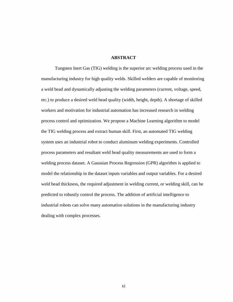
ABSTRACT

Tungsten Inert Gas (TIG) welding is the superior arc welding process used in the

manufacturing industry for high quality welds. Skilled welders are capable of monitoring

a weld bead and dynamically adjusting the welding parameters (current, voltage, speed,

etc.) to produce a desired weld bead quality (width, height, depth). A shortage of skilled

workers and motivation for industrial automation has increased research in welding

process control and optimization. We propose a Machine Learning algorithm to model

the TIG welding process and extract human skill. First, an automated TIG welding

system uses an industrial robot to conduct aluminum welding experiments. Controlled

process parameters and resultant weld bead quality measurements are used to form a

welding process dataset. A Gaussian Process Regression (GPR) algorithm is applied to

model the relationship in the dataset inputs variables and output variables. For a desired

weld bead thickness, the required adjustment in welding current, or welding skill, can be

predicted to robustly control the process. The addition of artificial intelligence to

industrial robots can solve many automation solutions in the manufacturing industry

dealing with complex processes.

1

I. INTRODUCTION

Background

Arc welding is the process of joining two or more metals together using electrical

energy. The two metals are heated by an electric arc and the atoms are fuse together.

Upon cooling, the metals coalesce into one piece that is as strong as the original material

strength. Arc welding is an essential process widely used in the manufacturing industry.

However, the decreasing workforce of skilled workers has significantly hindered

manufacturer’s ability to utilize the welding process. Certification for a professional

welder usually requires technical school instruction and can take several months. In

response, engineers have chosen to use industrial robots to replace the human worker and

increase productivity. Robot automation poses many advantages for simple processes;

however, these machines struggle to automate dynamic processes. Researchers have

attempted to overcome these limitations by equipping robots with artificial intelligence.

Machine learning algorithms enable robots to sense dynamic environments and make

intelligent changes like a human. The engineering challenge of this dissertation is to

automate the welding process using an industrial robot and extract human skill using a

machine learning algorithm.

Industrial Robots

An increase in technology and computing power in the last few decades led to the

use of industrial robots in the manufacturing industry. In 1961, the first prototype

industrial robot was produced by GM by combining three key technology waves: the

invention of Numerically Controlled Machines, popularity of the computer, and the

creation of integrated circuits (Wallen, 2008). Industrial robot development increased

2

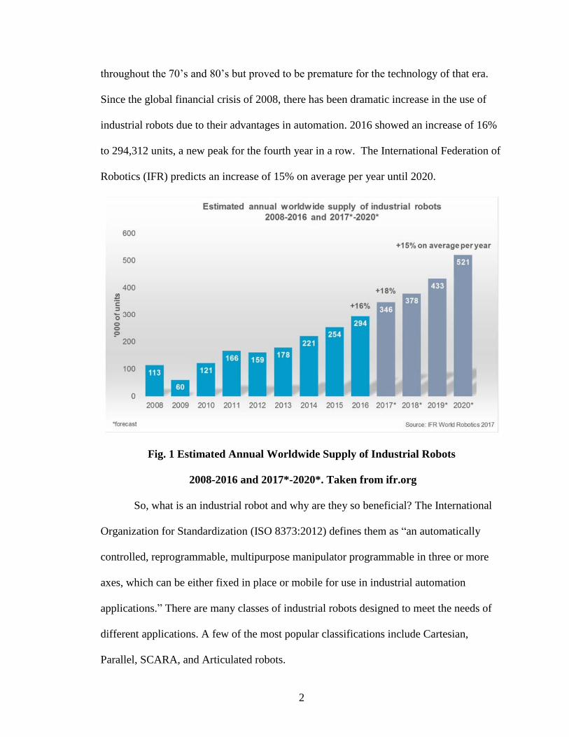
throughout the 70’s and 80’s but proved to be premature for the technology of that era.

Since the global financial crisis of 2008, there has been dramatic increase in the use of

industrial robots due to their advantages in automation. 2016 showed an increase of 16%

to 294,312 units, a new peak for the fourth year in a row. The International Federation of

Robotics (IFR) predicts an increase of 15% on average per year until 2020.

Fig. 1 Estimated Annual Worldwide Supply of Industrial Robots

2008-2016 and 2017*-2020*. Taken from ifr.org

So, what is an industrial robot and why are they so beneficial? The International

Organization for Standardization (ISO 8373:2012) defines them as “an automatically

controlled, reprogrammable, multipurpose manipulator programmable in three or more

axes, which can be either fixed in place or mobile for use in industrial automation

applications.” There are many classes of industrial robots designed to meet the needs of

different applications. A few of the most popular classifications include Cartesian,

Parallel, SCARA, and Articulated robots.

3

Fig 2. Types of Industrial Robots. Taken from ifr.org

Simpler-designed robots with only 4 axes and 4 degrees of freedom like the

Cartesian and SCARA robot can be used for performing simpler manufacturing tasks,

such as a pick and place or stamping operation. Articulated robots with 6 axes and 6

degrees of freedom are used for performing more complex manufacturing tasks, such as:

welding, grinding, painting, assembly, palletizing, heavy material handling, and

4

packaging. The trend of manufacturers integrating automation in the last decade is due to

the many benefits industrial robots possess including: high efficiency, high accuracy,

high quality, 24/7 operational time, hazardous environment immunity, high payload, and

reduced waste.

Of the 294,000 industrial robots used in the manufacturing industry worldwide,

the focus of this dissertation is on welding robots. Welding robots are most popular in the

Automotive and Metal industries.

Fig. 3 Estimated Annual Supply of Industrial Robots at Year-end by

Industries Worldwide 2014-2016. Taken from ifr.org

These two industries can account for 132,000 robots in 2016, which is 45% of the

total supply. All manufacturers can purchase from the most popular industrial robot

brands like Epson, Kawasaki, Fanuc, Kuka, and ABB. These robots can be easily

programmed to automate a simple process; however, a “stock” industrial robot will

struggle to produce consistent quality for dynamic processes under changing parameters,

5

noise, or uncertainties. An automated process failing on the manufacturing line will lower

the throughput and demand human interaction. Intelligent decision-making systems with

human-like capabilities are needed to increase industrial robot’s flexibility. Researchers

propose intelligent solutions by incorporating real time sensors and machine learning

algorithms. Intelligence is vital in a manufacturing process like arc welding where the

process parameters are changing and the system must deal with noise and uncertainties.

Welding

Joining two metals together is a process needed extensively in the manufacturing

industry. Arc welding is the most popular form of metal joining because the strength of a

good quality weld joint is equal to the initial material strength. Skilled welders use

different welding methods depending on the type of material, thickness of material,

available power source, type of weld joint, working environment, and the quality of weld

needed.

6

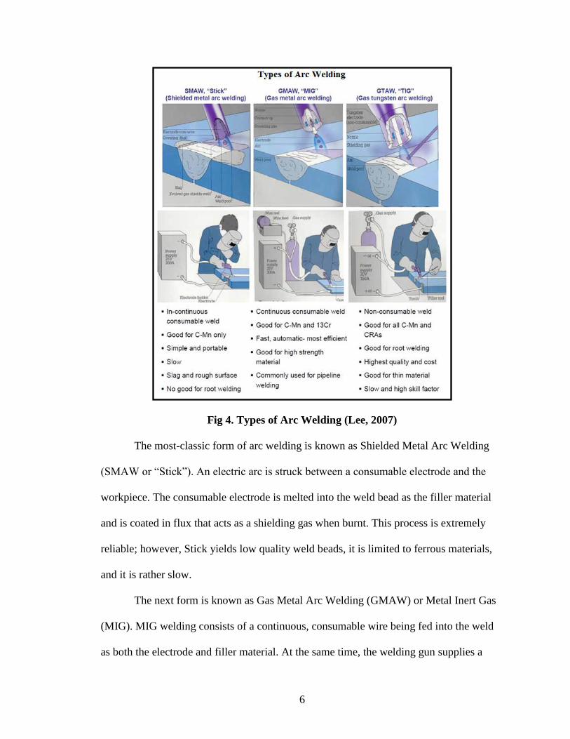
Fig 4. Types of Arc Welding (Lee, 2007)

The most-classic form of arc welding is known as Shielded Metal Arc Welding

(SMAW or “Stick”). An electric arc is struck between a consumable electrode and the

workpiece. The consumable electrode is melted into the weld bead as the filler material

and is coated in flux that acts as a shielding gas when burnt. This process is extremely

reliable; however, Stick yields low quality weld beads, it is limited to ferrous materials,

and it is rather slow.

The next form is known as Gas Metal Arc Welding (GMAW) or Metal Inert Gas

(MIG). MIG welding consists of a continuous, consumable wire being fed into the weld

as both the electrode and filler material. At the same time, the welding gun supplies a

7

protection gas to prevent weld bead contamination. The MIG process is easy to learn, the

welding speeds are fast, and it yields good quality weld beads. However, MIG is limited

to thick materials and mostly only ferrous metals. Also, welding parameters current and

wire feed rate are constant and not designed to adjust during the welding process.

Lastly, Gas Tungsten Arc Welding (GTAW or “TIG”) is the most complex

process of the three. A non-consumable electrode is used to strike an arc and heat the

weld bead area while being protected by inert gas. During the process, the welding torch

is moved at a given speed, torch angle, and distance from the workpiece. At the same

time, consumable metal is fed into the weld bead area for reinforcement if it is needed.

Concurrently, the current can be adjusted to control heat flow. The skill needed of a TIG

welder to simultaneously control the current with a foot pedal, move the electrode torch

with one hand, and add filler material with the opposite hand is what makes this method

difficult to learn. Ironically, the dynamic control of the welding parameters is what

welders prefer once the skill is mastered. TIG welding’s active-parameter control enables

the welder to gain the most heat control of the weld pool compared to Stick or MIG.

Consequently, TIG welding is the preferred arc welding process for thin metals,

nonferrous metals, and most importantly when weld quality is important (Patel, 2014)

Manual TIG welding is a dynamic manufacturing process where the input

welding parameters directly affect the output welding quality. There are many input

welding parameters that the welder is responsible for setting and controlling: 1 Tungsten

electrode material type and diameter, 2 ceramic gas cup size, 3 torch orientation angle, 4

torch travel speed, 5 arc distance, 6 inert gas type, 7 gas flow rate, 8 amount of current, 9

AC balance, etc.

8

Fig 5. TIG Welding Process Diagram (Patel, 2014)

A professional welder can generally preselect ideal parameter settings based off

the material type, thickness, and desired weld quality. Once the welding arc is struck with

the workpiece under the initial parameters, the welder actively monitors the dynamic

weld pool and intelligently adjusts the welding parameters current, travel speed, and arc

distance accordingly. A skilled welder’s intelligent response can decrease inconsistency

in weld bead quality. The weld bead quality can be measured by the 3d weld pool

convexity, the weld bead width, depth of penetration, or mechanical strength. Given a

desired weld bead quality, we attempt to extract human welder’s parameter changing

skill.

Automating a manufacturing process using an industrial robot, the system gains

many advantages. An ABB robot is capable of repeating a programmed weld path with

the accuracy of +/- 0.03mm and up to 2.5m/s (ABB, 2017). Programmers use these

advantages to simulate a virtually perfect human welder. First, we can move the welding

torch at a constant speed. Second, we can program the welding torch at a constant torch

9

angle and constant arc distance. Third, we can control the amount of current discretely.

Fourth, we can repeat the same weld path accurately each time. Once constant input

parameters are established, one isolated input parameter can be adjusted. Finally, sensors

can be used to measure and analyze the relationship between an isolated input parameter

and the resultant weld bead quality.

Artificial Intelligence & Machine Learning

Artificial Intelligence is the science of “creating computer programs or machines

capable of behavior we would regard as intelligent if exhibited by human.” Early

computer science pioneers found success in the 50s 60s by creating computer vision

algorithms and natural language recognition (Kaplan, 2016). However, progress was

plagued by technology limitations. An increase in computational power and large data

sets has revitalized AI development. An increase in AI use can be witnessed in everyday

lives. For example, Google image searches or smartphone speech recognition are two

basic technologies utilizing large datasets. More complex ideas being developed today

include self-driving cars, humanoid robots, and intelligent healthcare systems.

Scientists seek to add intelligent abilities to a computer system through reasoning,

knowledge, planning, learning, natural language processing, and perception (Russel,

1995). Intelligent capabilities can be used by machines to automatically solve complex

problems. In order to solve a problem using a computer (or machine), we need an

algorithm. According to Alpaydin (2014), “an algorithm is a sequence of instructions that

should be carried out to transform the input to output.” The coupling of computer

algorithms and large data sets has led to the development of machine learning algorithms.

Machine Learning (ML) is the process of defining a process model, learning how to

10

optimize the parameters, and ultimately gain descriptive knowledge of a process or make

predictions in the future. Optimization and predictability are two major attributes that can

be utilized by industrial robots since companies are increasingly looking for automated

solutions.

Taking a computer science tool that typically uses theoretical datasets and

applying it to a practical manufacturing process can be challenging. For example:

datasets can include many variable, relationships of inputs and outputs may be nonlinear,

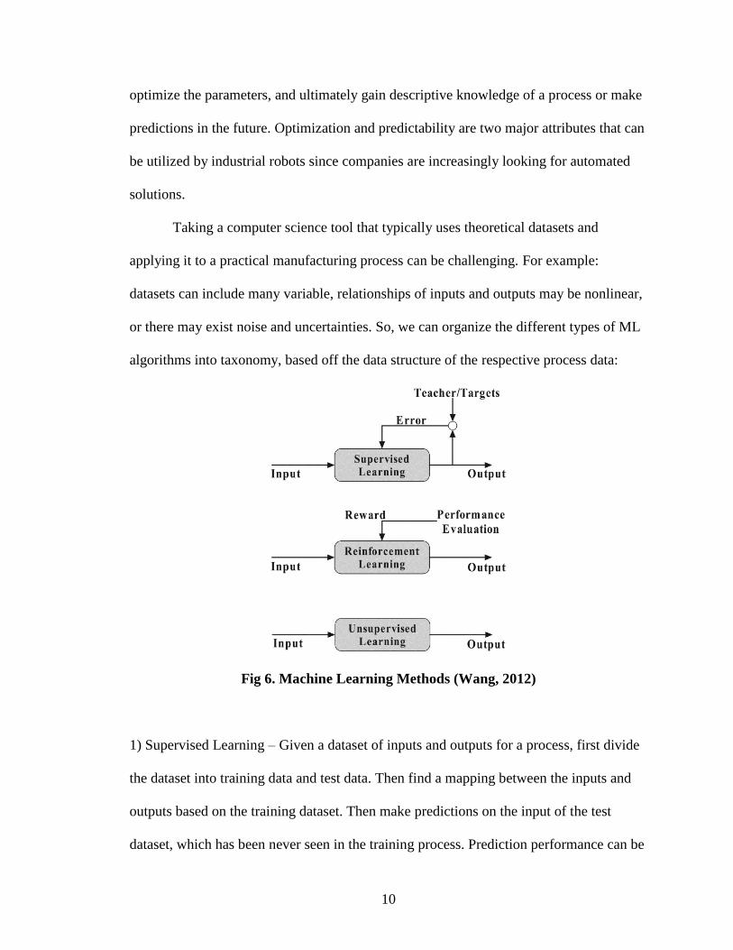
or there may exist noise and uncertainties. So, we can organize the different types of ML

algorithms into taxonomy, based off the data structure of the respective process data:

Fig 6. Machine Learning Methods (Wang, 2012)

1) Supervised Learning – Given a dataset of inputs and outputs for a process, first divide

the dataset into training data and test data. Then find a mapping between the inputs and

outputs based on the training dataset. Then make predictions on the input of the test

dataset, which has been never seen in the training process. Prediction performance can be

11

measured since the output of the training data is already given. Examples of supervised

learning algorithm techniques include: ANOVA, DOE Taguchi, classification, regression,

support vector machines, neural networks, and decision tree.

2) Unsupervised learning – Given a dataset of inputs and outputs for a process, extract

patterns or relationships in the input data. Since this method is open looped, there is no

feedback from the environment. Examples of unsupervised learning algorithm techniques

include: self-organizing maps, clustering.

3) Reinforcement Learning – Given an online system, input and output data is produced

through interaction with the environment. This approach learns a mapping through trial

and error. So, every input action yields a feedback from the environment. The goal is to

maximize the expected cumulative reward. Examples of reinforcement learning algorithm

techniques include: temporal-difference, deep learning.

12

II. LITERATURE REVIEW

Neural Networks

Preliminary studies were done by W. Zhang & Y. Zhang (2012) to model the

human welding process using a statistical technique called autoregressive with exogenous

terms model, similar to “moving averages.” In this experimental setup, a laser camera-

vision system is set up to since the real time 3D weld pool surface of a human welder,

TIG welding a steel pipe. The input to the model is the sensing of the 3D pool surface

quality (weld pool length, width, and convexity). The output of the system is the changes

the human welder makes to the welding parameters (speed, current, and arc distance). It

was discovered that the linear model was insufficient to model a nonlinear welding

process. However, key findings were made that many researchers used later: 1) A human

welder makes adjustments on the welding parameters based on the real time and previous

weld pool surface from approximately 1.5s to 3s previously. 2) A human welder also

makes adjustments on the welding parameters based on the previous adjustments he has

made 1s prior. These characteristics show the arc welding process is a nonlinear and

time-delayed process.

Then, Wang & Liu teamed up with W. Zhang and Y. Zhang (2012) at the

University of Kentucky and took a non-linear modeling approach to modeling the

welding process, called least squares algorithm. The goal here was to predict weld bead

penetration in the form of backside weld bead width. So, Wang et al. used the same TIG

welding process and laser vision system as W. Zhang and Y. Zhang (2012), but modeled

the data differently. The input parameters consisted of real time 3d weld pool surface

quality (weld pool width, length, convexity). Output of the system was the backside

13

width of the resultant weld bead. The least square algorithm was capable of predicting

the backside width with an acceptable variance of s^2=0.39 mm^2. This proved that data

could be extracted from the welding process to predict weld bead quality.

Further research at the University of Kentucky was conducted by Liu, W. Zhang,

and Y. Zhang (2013). The first intelligent human welder modeling and control method

was accomplished using an artificial neural network (ANN). Again, the same TIG

welding process and laser vision system was used for experimentation, but the data

structure was modeled different. The input parameters consist of the real time 3D pool

surface quality extracted (weld pool width, length, and convexity). An Adaptive Neuro-

Fuzzy Inference System (ANFIS) technique was used to learn the welding process and

output the current, with an RMS error of 0.517A. Once the model of the system was

learned, the input and output parameters were swapped in order to control and optimize

weld quality. Given a desired weld bead width, the algorithm suggests an adjustment to

the welding parameters (current, speed, arc length). This study established a foundation

to add human welder’s intelligence into a robotic welding system.

The ANFIS model based predictive control uses nonlinear optimization, which

are not preferred for online industrial applications. Liu and Y. Zhang (2014) then used the

nonlinear ANFIS model to train the system and a linear, model predictive control (MPC)

algorithm to optimize the process. Open-loop control experiments were conducted to

show the controller’s ability to achieve a desired weld bead quality under various

disturbances and initial conditions.

Eventually, Liu, Y. Zhang, and Y. Zhang (2015) accomplished a modeling and

control technique for an online intelligent arc welding system. A dynamic nonlinear

14

ANFIS model was used to train the system and utilized as a nonlinear controller. This

technique achieved faster response time then the linear system used by Liu and Y. Zhang

(2014). The achievement from a supervised learning system to a reinforcement learning

system makes this algorithm useful for practical industry applications.

Wang and Li (2014) were able to borrow data from the University of Kentucky’s

lab and apply three different BP-ANNs to optimize weld bead quality. Wang’s model was

based off of 11 input data parameters: weld pool length, width, half length, half width,

height, section area, concavity, radius, current, arc length, and speed. The output for each

system was backside weld bead width and height. The model was trained using a back-

propagation neural network (BPNN), a principle component analysis based back-

propagation neural network (PCABPNN), and a global best adaptive mutation particle

swarm optimization based back-propagation neural network (GBAMPSO-BPNN) model.

The GBAMPSO-BPNN model was capable of predicting the weld bead width, with an

RMS error of 0.3872mms.

Baskoro, Tandian, Haikal, Edyanto, & Saragih (2016) also applied a BP-ANN to

analyze an automated TIG welding process on stainless steel. A stepper motor was used

to traverse the workpiece at a constant speed and automate the process. A charge-coupled

device (CCD) camera was used to measure the top weld bead with and a ruler was used

to measure the backside weld bead width. Experiments were conducted at a constant

speed and constant current while the CCD measured the top bead width. The ANN was

used to train the model and predict the backside weld bead quality. Baskoro et al. provide

minimal description of the ANN technique other than the fact that it uses back-

propagation. For a target backside weld bead width of 3mm, an absolute error of 0.11mm,

15

0.09mm, and 0.12mm is achieved for only three experiments. This experimental design

using constant current and speed does not show much promise in modeling a dynamic

welding process with changing speed or current.

Another ANN approach by Vinas, Cabrera, and Juarez (2016) was modeled after

an automated MIG welding process using a Fuzzy ARTMAP technique. The architecture

of the ANN uses a combination of Fuzzy Logic and Adaptive Resonance Theory.

Experiments were conducted using a KUKA industrial robot to vary the input parameters

(arc distance, speed, and current). A CCD camera was used to measure the output weld

bead height and width. Automated welding, ANN training, and ANN testing were all

conducted online in 4.5minutes. An average prediction error of 0.169mms was achieved.

A deep neural network (DNN) approach was used by Keshmiri, Zheng, Feng,

Pang, and Chew (2015) to estimate weld bead quality of a MIG welding, SMAW

welding, and TIG welding system. DNN is simply the parallel use of many ANNs. In

Keshmiri et al.’s design four-hidden-layer architecture; the first three layers utilize the

sigmoid function and the fourth layer uses a linear transformation to produce the final

output of the system. Input parameters (voltage, current, speed, and wire-speed were used

to predict the output parameters (depth of penetration and weld bead width). RMSE of

the predicted width for four different datasets were achieved: 0.115mm, 0.15mm,

0.153mm, and 0.124mm. The study shows that DNN’s are capable of modeling various

welding process and produce good results with a limited number of data points.

16

Support Vector Machines

While NNs have proven to dominate the welding optimization research, others

have used statistical learning strategies to model the process. Li, Gao, Wu, Hu, and Wang

first used a Support Vector machine to classify the weld quality of a Metal Active Gas

(MAG) welding process. In this process, the weld shape was not a straight-line weld like

all other researchers, but the input and output variables were similar. Li et al. kept arc

distance, speed, gas flow, and at constant settings while changing the one input variable

current. The goal was to model the relationship with the output weld quality, measured by

a vision-based sensor. The classifier was capable of successfully predicting the groove

state, or weld bead quality, 85% of the time.

So, then Dong, Huff, Cong, Zhang, and Chen (2016) adopted the classification

technique and designed their own Support Vector machine algorithm. TIG welding

experiments were conducted with Liu et al.’s (2013) model for predicting characteristic

performance was used: the input variables were welding parameters, previous welding

parameters, and previous characteristic performance, while the output variable was the

current characteristic performance. More specifically; Dong and Huff’s input variables

were current, previous current and previous weld bead width while the output variable

was weld bead width. Classification of weld bead width was successfully predicted at

95%. Classifiers have proven to model the welding process for a range of values, but not

a discrete value.

Gaussian Process Regression

Next, Dong, Cong*, Liu, Zhang, and Chen (2016) used a regression technique to

model the welding process using Gaussian Process Regression (GPR). GPR regression of

17

welding data had briefly been investigated by D. Sterling, T. Sterling, Zhang, and Chen

(2015) at Texas State University. The GPR was first used to model the welding process

and optimize the parameters for weld bead strength. Dong was able to design a more

complex algorithm using Liu and Zhang’s (2014) modeling technique for predicting

characteristic performance. Using input variables: previous width, previous current, and

previous speed; Dong modeled the relationship with output variables width and

convexity. A maximum prediction error and minimum prediction error of 0.1017mm and

0.0067mm were achieved for width. And a maximum prediction error and minimum

prediction error of 0.0182mm and 0.0024mm were achieved for convexity. The GPR

proved capability of modeling the welding process for a discrete mean value with a

specified variance. Further research by Dong et al. (2017) was done to equip the GPR

algorithm with a Bayesian Optimization Algorithm (BOA). Upper confidence bound and

lower confidence bound techniques were applied to the predicted mean and variance. By

incorporating the BOA, Dong was then capable of modeling the process in real time.

Origination of Thesis

Artificial Intelligence has increased industrial robot welding capabilities through

several machine learning algorithms. Neural Networks based off back propagation have

dominated the welding process modeling and optimization. However, there is a lack of

other machine learning techniques used to solve the problem. Dong and Huff used other

techniques such as SVM and GPR to model and predict the weld bead quality

successfully.

18

Table 1. Machine Learning Algorithms used to Model the Welding Process

Author(s) Algorithm Technique

Welding

Process

Material Output Error

W. Zhang, Y.

Zhang

(2012)

Regression Least Square TIG steel width s2 = 0.39mm2

Liu, W.

Zhang, Y.

Zhang

(2013)

ANN Fuzzy Logic TIG steel current

RMSE = 0.67A

max = 3.83A

Liu, Y.

Zhang

(2014)

ANN Fuzzy Logic TIG steel width max = 0.5mm

Liu, W.

Zhang, Y.

Zhang

(2015)

ANN Fuzzy Logic TIG steel width

RMSE = 0.60A

max = 4.17A

Wang, Li

(2014)

ANN

Back

Propagation

arc, smaw,

TIG

steel width RMSE = 0.3872

Keshmiri et

al. (2015)

DNN

Back

Propagation

TIG,

SMAW

steel,

SS304

width

.124mm or

2.52%

Baskaro et al.

(2016)

ANN

Back

Propagation

TIG SS304 width .09mm or 2%

Vinas et al.

(2016)

ANN

Back

Propagation

MIG steel width 0.169mm avg

19

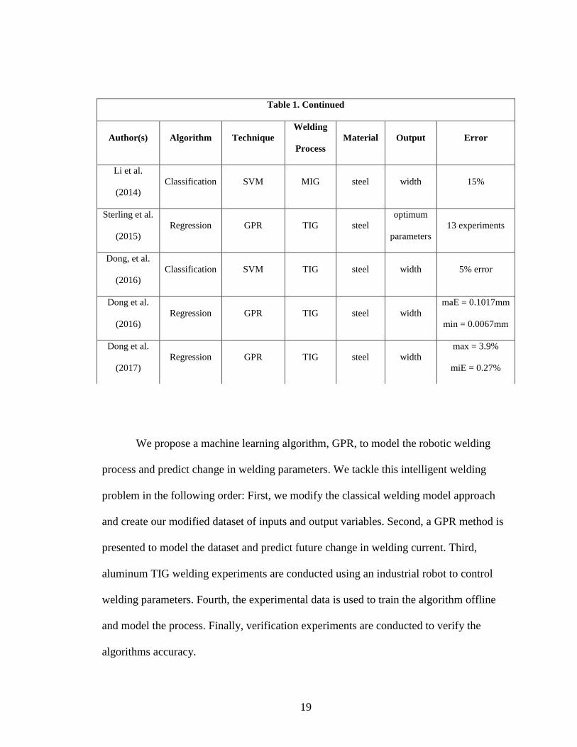
We propose a machine learning algorithm, GPR, to model the robotic welding

process and predict change in welding parameters. We tackle this intelligent welding

problem in the following order: First, we modify the classical welding model approach

and create our modified dataset of inputs and output variables. Second, a GPR method is

presented to model the dataset and predict future change in welding current. Third,

aluminum TIG welding experiments are conducted using an industrial robot to control

welding parameters. Fourth, the experimental data is used to train the algorithm offline

and model the process. Finally, verification experiments are conducted to verify the

algorithms accuracy.

Table 1. Continued

Author(s) Algorithm Technique

Welding

Process

Material Output Error

Li et al.

(2014)

Classification SVM MIG steel width 15%

Sterling et al.

(2015)

Regression GPR TIG steel

optimum

parameters

13 experiments

Dong, et al.

(2016)

Classification SVM TIG steel width 5% error

Dong et al.

(2016)

Regression GPR TIG steel width

maE = 0.1017mm

min = 0.0067mm

Dong et al.

(2017)

Regression GPR TIG steel width

max = 3.9%

miE = 0.27%

20

III. PROPOSED SOLUTION

Process Modeling

Arc welding is a dynamic process with many complex variables that make it

challenging to model. Most significantly; there are several welding parameters (WP)

(current, voltage, speed, arc distance, etc.) that determine the quality of the weld bead

(WQ) (width, depth of penetration, convexity, tensile strength, etc.) The input and output

parameters strongly correlate with each other; however, it is a nonlinear relationship.

Also, the process involves uncertainties including metallurgy, heat transfer, chemical

reaction, arc physics, and electromagnetism. Hence why Wang and Li (2014) label the

arc welding process as a multi-input, multi-output (MIMO), nonlinear, time-varying, and

strong coupled process.

In order to model the process, we must first understand the skill needed by human

welders. The principle of human welder’s intelligence and control is briefly described:

Given a welding task of joining two metals together at a joint, the human must first

evaluate the properties of the workpiece material, the workpiece thickness, and determine

a desired weld bead quality (WQd). Based off prior experience, some initial estimation of

welding parameters (WP) is determined. After an initial welding arc is struck on the

workpiece, the welder evaluates the actual weld bead quality (WQ) with his eyes. Over

time, t, the real time observed data WQ(t), prior observed data WQ(t-1), and prior

welding parameters WP(t-1) used to determine the necessary control action, or change in

WP. The change in WP is human skill required for controlling good quality welds and a

vital skill industrial robots lack.

21

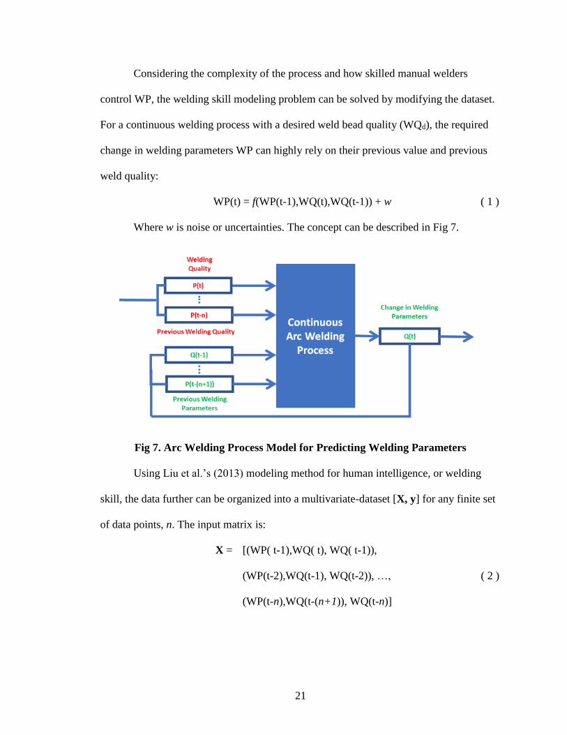
Considering the complexity of the process and how skilled manual welders

control WP, the welding skill modeling problem can be solved by modifying the dataset.

For a continuous welding process with a desired weld bead quality (WQd), the required

change in welding parameters WP can highly rely on their previous value and previous

weld quality:

WP(t) = f(WP(t-1),WQ(t),WQ(t-1)) + w ( 1 )

Where w is noise or uncertainties. The concept can be described in Fig 7.

Fig 7. Arc Welding Process Model for Predicting Welding Parameters

Using Liu et al.’s (2013) modeling method for human intelligence, or welding

skill, the data further can be organized into a multivariate-dataset [X, y] for any finite set

of data points, n. The input matrix is:

X = [(WP( t-1),WQ( t), WQ( t-1)),

(WP(t-2),WQ(t-1), WQ(t-2)), …,

(WP(t-n),WQ(t-(n+1)), WQ(t-n)]

( 2 )

22

The output matrix includes only one n x 1 vector:

y = [WP(t), WP(t-1), …, WP(t-n)] ( 3 )

Once a dataset [X,y] of a process is obtained a model can be trained to learn the

relationship between the inputs and output.

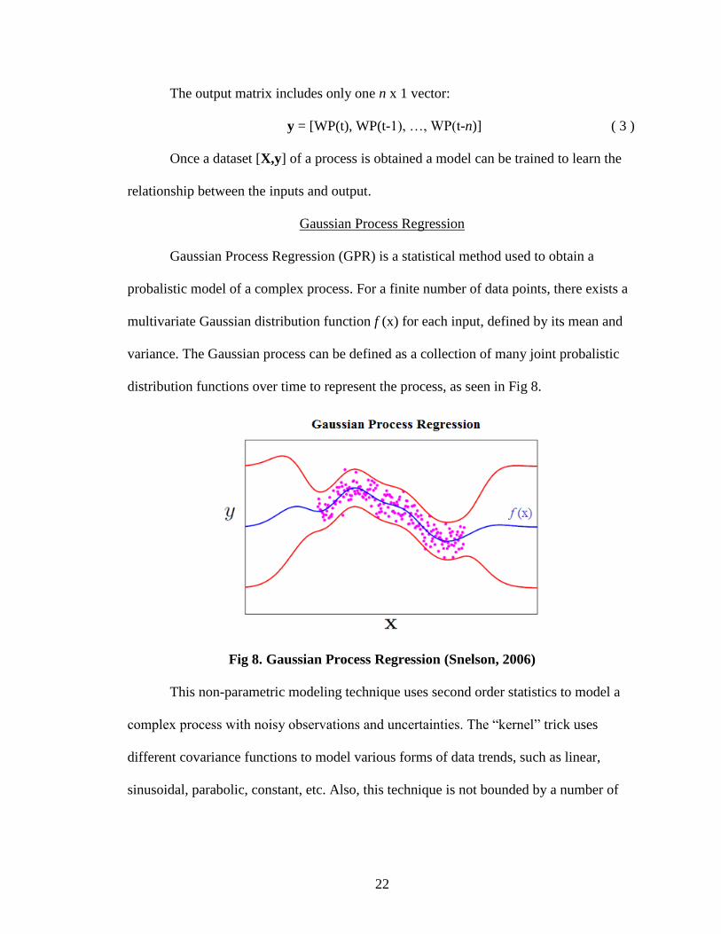
Gaussian Process Regression

Gaussian Process Regression (GPR) is a statistical method used to obtain a

probalistic model of a complex process. For a finite number of data points, there exists a

multivariate Gaussian distribution function f (x) for each input, defined by its mean and

variance. The Gaussian process can be defined as a collection of many joint probalistic

distribution functions over time to represent the process, as seen in Fig 8.

Fig 8. Gaussian Process Regression (Snelson, 2006)

This non-parametric modeling technique uses second order statistics to model a

complex process with noisy observations and uncertainties. The “kernel” trick uses

different covariance functions to model various forms of data trends, such as linear,

sinusoidal, parabolic, constant, etc. Also, this technique is not bounded by a number of

23

input parameters. Hence GPR is a robust tool that can be used to model the multi-input,

multi-output (MIMO), nonlinear, time-varying, and strong coupled TIG welding process.

For a Gaussian Process f(x), a set of multivariate Gaussian random variables F =

{f(x1), f(x2),…, f(xN)] can be defined over X with any finite set of N points {xi∈X}𝑖−1𝑁

where f(xi) has the value of the latent function f(x) at xi∈X and X is defined over ℝD. f(x)

is completely specified by its mean function m(x) and covariance function k(x,x´): f(x) ~

𝒢𝒫(m(x),k(x,x´)) where x and x´ are two arbitrary variables in X.

For a model y = f(x) + w and w ~ N(0, σ𝑛𝟐), the covariance function is

cov(yi,yj) = k(xi,xj) + σn2δij, where δij is the Kronecker delta which is one, if i = j and zero

otherwise. The joint distribution of the observed data set (X, y) and predicted data set

(𝑿∗, 𝐲∗) is

[

𝐲𝐲∗

] ~ N (0, [𝐾(𝐗, 𝐗) + σn

2I 𝐾(𝐗, 𝐗∗)𝐾(𝐗∗, 𝐗) 𝐾(𝐗∗, 𝐗∗)

])

( 4 )

Where K(X´,X´´) (X´ and X´´ refer to X and 𝑿∗) is the covariance matrix whose

element Kij in ith row and jth column equals to k(xi´,xj

´´). By deriving the conditional

distribution, we can obtain:

(y* |X,y,X*) ~ N(μ(y*),V(y*))

μ(y*) = E[y*|X,y,X*] = K(X*,X)[K(X, X) + σn2I]-1y

V(y*) = K(X*, X*) – K(X*, X) [K(X, X) + σn2I]-1K(X, X*)

( 5 )

( 6 )

( 7 )

Where μ(y*) is the predicted mean for y* and V(y*) is the predicted variance. The

covariance function k(x,x´) is a key for determining a GPR model. Among various forms

of covariance functions, a commonly-used one is the Squared Exponential kSE(x,x´)

which is:

24

kSE(x,x´) = σ2 exp(−|𝐱−𝐱′|^2

2𝑙2 ) ( 8 )

Where l is a characteristic length-scale factor controlling how close x and x´ are

and 𝜎2 is the amplitude of the variance. For each covariance function, there are some

hyperparameters θ such as l and 𝜎 for kSE. The goal of model construction is to find a

covariance function k(x,x´,θ) which fits the data set (X,y) best. Suppose f(x) is a

candidate latent function, f in short, for the given data set, the posterior probability is:

p( f |X,y,H,θ) = 𝑝(𝐲,𝐗,𝑓,𝐻,θ) 𝑝(𝑓|𝐗,𝐻,θ)

𝑃(𝐲|𝐗,𝐻,θ) ( 9 )

Where H is the hypothesis on the structure of the covariance function, θ is the

hyperparameters, X, y are the sample data sets and

p(y|X,H,θ) = ∫ p(y|X, f,H,θ) p( f |X,H,θ)df ( 10 )

is the marginal likelihood that refers to the marginalization over the function f.

As mentioned above, in the Gaussian Process Regression f (x) is not given

explicitly. Thus, p(y,X,H,θ) actually refers to the likelihood of H and θ given the data set

(X,y). The Gaussian assumption makes it possible to derive the analytical solution of the

log marginal likelihood:

log P(y|X,H,θ) = - 1

2log|(K+σn

2I)| - 1

2yT(K+σn

2I)-1y - 𝑛

2log2π ( 11 )

Therefore the hyperparameters θ in a covariance function H can be optimized by

maximizing the marginal log likelihood:

θ*= argmaxlog p(y|X,H,θ) ( 12 )

This optimization problem can be solved using different techniques such as

Conjucted Gradient Algorithm or evolutionary algorithms. Nelder-Mead(Simplex)

25

method is utilized which is effective and uses only the value of log p(y|X,H,θ). Once

k(x,x´,θ) is known, equation (7) can be used to make a prediction for a new input x*.

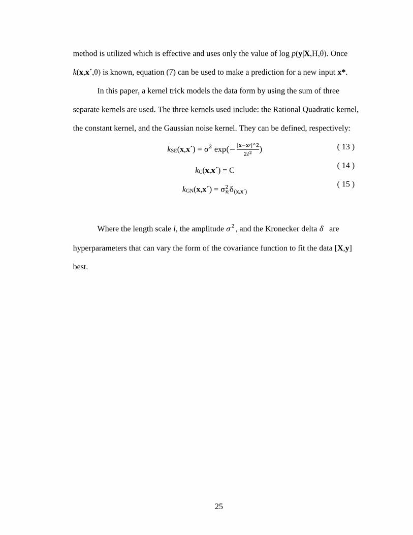
In this paper, a kernel trick models the data form by using the sum of three

separate kernels are used. The three kernels used include: the Rational Quadratic kernel,

the constant kernel, and the Gaussian noise kernel. They can be defined, respectively:

kSE(x,x´) = σ2 exp(−|𝐱−𝐱′|^2

2𝑙2 )

kC(x,x´) = C

kGN(x,x´) = σ𝑛2 δ(𝐱,𝐱´)

( 13 )

( 14 )

( 15 )

Where the length scale l, the amplitude 𝜎2 , and the Kronecker delta 𝛿 are

hyperparameters that can vary the form of the covariance function to fit the data [X,y]

best.

26

IV. EXPERIMENTATION

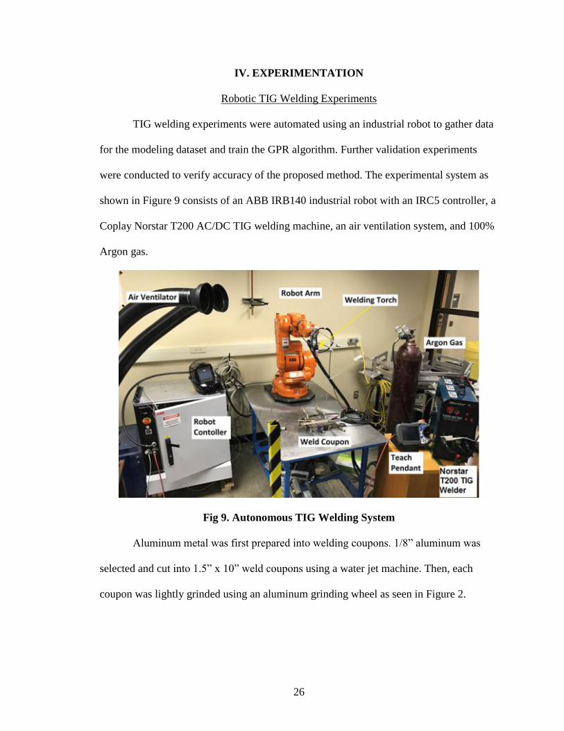
Robotic TIG Welding Experiments

TIG welding experiments were automated using an industrial robot to gather data

for the modeling dataset and train the GPR algorithm. Further validation experiments

were conducted to verify accuracy of the proposed method. The experimental system as

shown in Figure 9 consists of an ABB IRB140 industrial robot with an IRC5 controller, a

Coplay Norstar T200 AC/DC TIG welding machine, an air ventilation system, and 100%

Argon gas.

Fig 9. Autonomous TIG Welding System

Aluminum metal was first prepared into welding coupons. 1/8” aluminum was

selected and cut into 1.5” x 10” weld coupons using a water jet machine. Then, each

coupon was lightly grinded using an aluminum grinding wheel as seen in Figure 2.

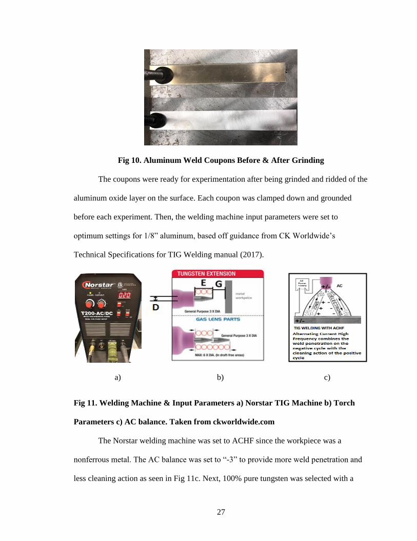
27

Fig 10. Aluminum Weld Coupons Before & After Grinding

The coupons were ready for experimentation after being grinded and ridded of the

aluminum oxide layer on the surface. Each coupon was clamped down and grounded

before each experiment. Then, the welding machine input parameters were set to

optimum settings for 1/8” aluminum, based off guidance from CK Worldwide’s

Technical Specifications for TIG Welding manual (2017).

a) b) c)

Fig 11. Welding Machine & Input Parameters a) Norstar TIG Machine b) Torch

Parameters c) AC balance. Taken from ckworldwide.com

The Norstar welding machine was set to ACHF since the workpiece was a

nonferrous metal. The AC balance was set to “-3” to provide more weld penetration and

less cleaning action as seen in Fig 11c. Next, 100% pure tungsten was selected with a

28

diameter, measurement D in Fig. 11, of 3/32”. The welding torch was setup with a #7

ceramic cup and the tungsten extension distance, or measurement E in Fig. 11, was set to

9/32”. Current on the machine was set to the initial current of each experiment.

After the weld coupons were prepared and the machine parameters were set, a

robot program was written using the program RobotStudio to carry out the welding

experiments. ABB’s robot programming language RAPID was used.

Fig 12. Robot Program Parameters

The welding torch was programmed to move to a point in space, point A seen in

Fig.12, at the beginning of the weld coupon. The vertical torch angle was set to 75° from

the horizontal weld plane. Then the arc distance, point G seen in Fig. 12, was set to 0.05”.

Finally, the welding torch was programmed to move in a straight line to point B in Fig 12

with a constant speed of 0.1181”, or 3mm/s.

29

A total of 50 welding experiments were conducted, Fig. 14. For each experiment,

the welding current was set to an initial random current value while traveling the first

3.3”, then adjusted to a second random current value while traveling the next 3.3”, and

then adjusted to a third random current value for the last 3.3”. For example, in Fig 13 the

current in welding experiment #4 is initially 79A, changes to 83A, and then changes to

55A.

Fig 13. Experiment #4

A total of 50 welding experiments were conducted as seen in Fig 14:

a) Experiment 1-10 b) Experiment 11-20

30

c) Experiment 21-30 b) Experiment 31-40

e) Experiment 41-50

Fig 14. Training Experiment Weld Coupons a) Experiments 1-10 b) Experiments

11-20 c) Experiments 21-30 d) Experiments 31-40 e) Experiments 41-50

31

After the experiments were completed, an image processing code was used to

measure the weld bead width.

Fig 15. Shading in Microsoft Paint

A 1280 x 960 pixel resolution photo was taken of the top of the weld bead. Then,

Microsoft Paint was used to manually shade everything pure black in the picture that was

not part of the weld bead. Using computer software Matlab, the code interposed which

pixels were pure black and which were weld bead. For a given horizontal row of pixels,

the number of weld bead pixels yielded the pixel width of the weld bead. The pixel width

was then calibrated with the pixel length of 1” on a ruler. Finally, a weld bead width

value was measured for each current value. This method was used for the first five

experiments. The width was also measured using a manual set of calipers. Since the

manual shading was required for image processing and the width measurements with the

calipers were more straight forward, caliper measurements were performed for all the

32

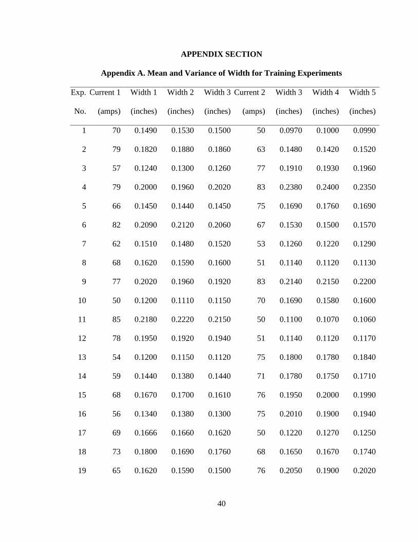
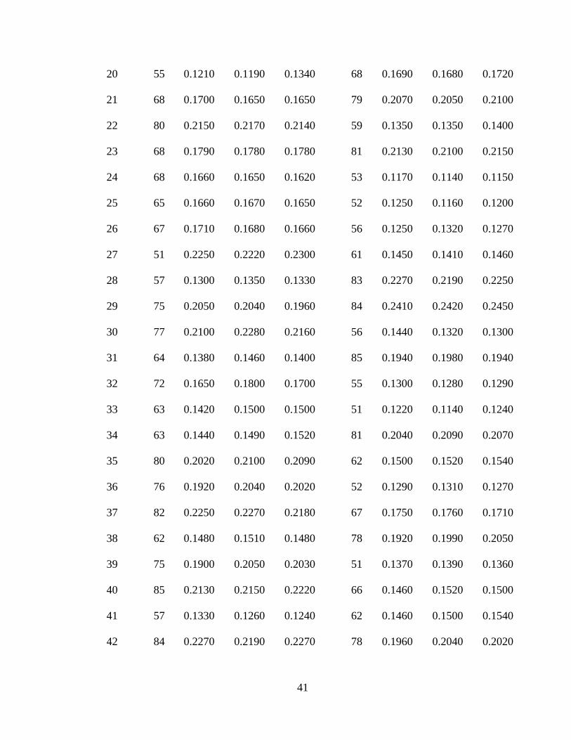
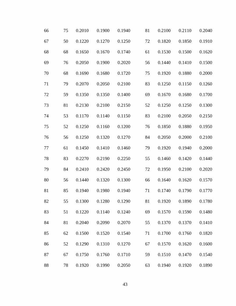
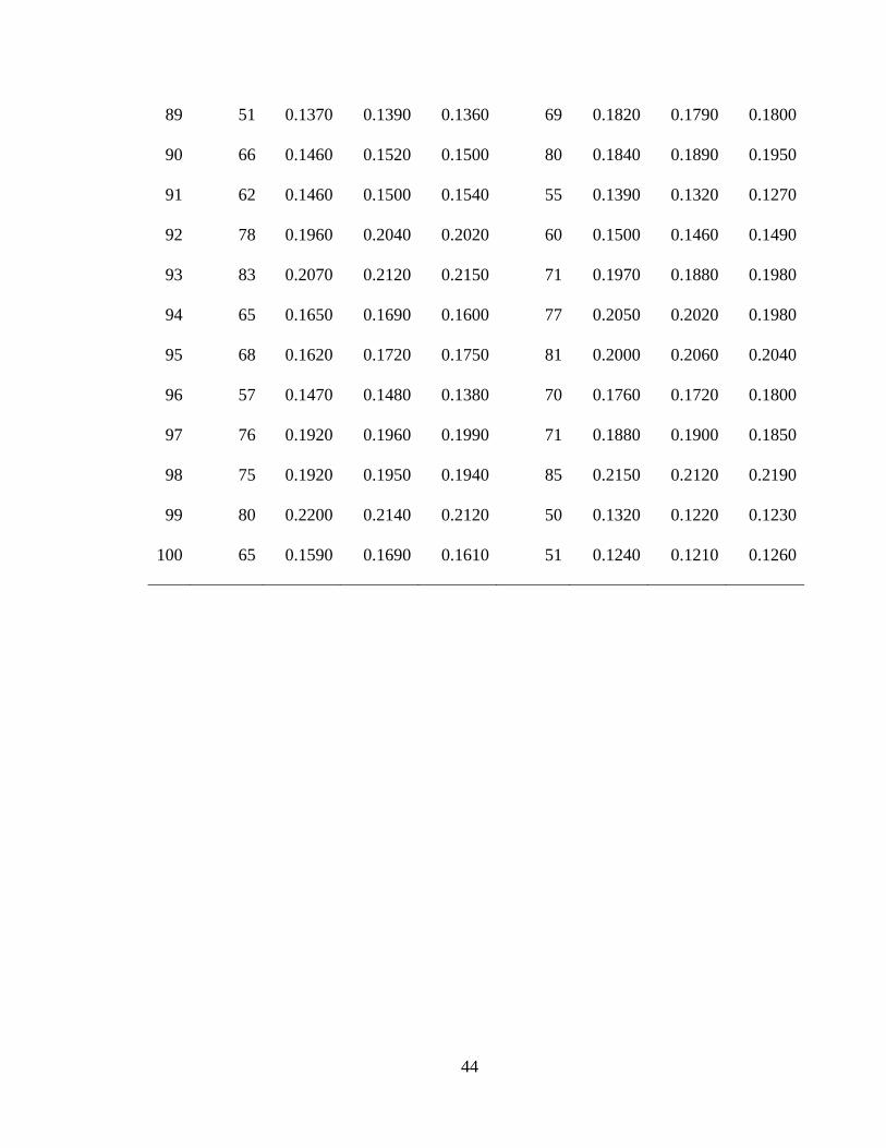
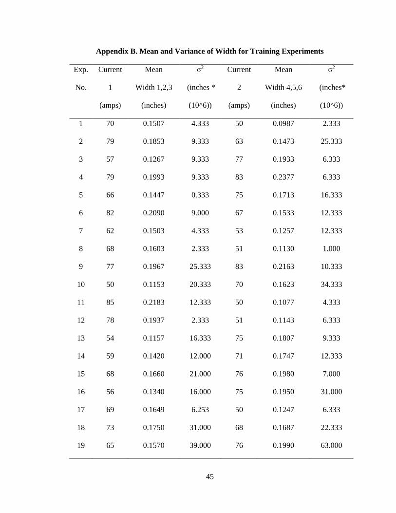
data. For each current value, three width measurements were recorded, found in

Appendix A. The width measurement’s mean and variance can be found in Appendix B.

Welding currents and weld bead widths from experiments 1-50, 2 datasets each, were

used to create the data set [x,y] of size 100x4. The multivariable input [x] has a size of

100x3 and the output variable [y] has a size 100x1. 90/100 randomly selected data points

in the data set [x,y] were used to create the training data set [trainX, trainY] and the

remaining 10/100 data points were used for the testing data set [testX, testY].

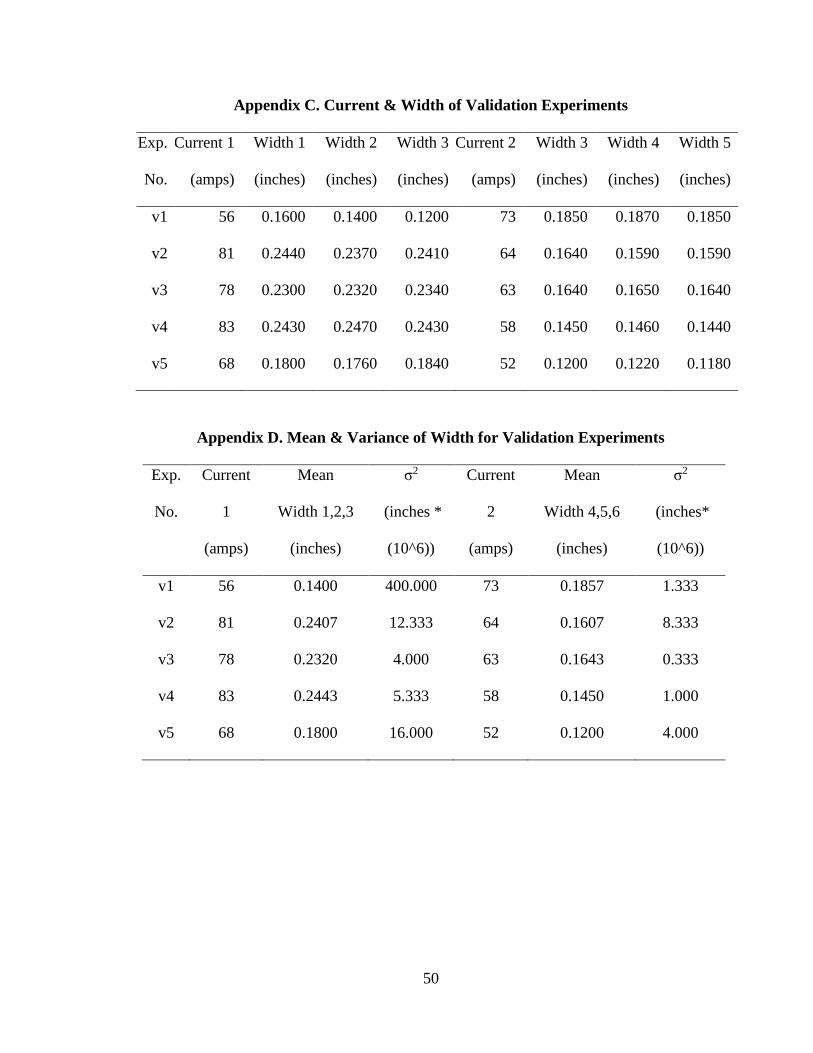
Finally, five more validation experiments were performed. However, the initial

current was set to some random value while traveling the first 5” and then adjusted the

algorithm’s predicted current value for the last 5”. The previous current, current, previous

width, and width were used to create the new testing data set [valX, valY] of size 5x4.

The raw data can be found in Appendix C and the mean and variance can be found in

Appendix D.

Fig 16. Validation Experiments #1-5

33

V. RESULTS

Training Results

A modeling algorithm was written on Matlab, equipped with an open source

toolbox: “Gaussian Process Regression for Machine Learning.” (Rasmussen & Nickisch,

2017) The following kernel functions were used with their respective optimal

hyperparameters.

Table 2. Covariance Functions

Name Function

covConst Constant

covSEiso Squared Exponential

covNoise Gaussian Noise

The GPR model was trained using [trainX,trainY]. Applying the GPR model to

the input [testX], predictions were made of output variable [testY]. The prediction results

are shown in Table 3.

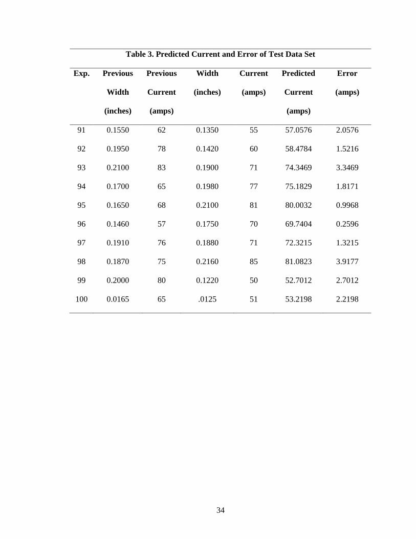
34

Table 3. Predicted Current and Error of Test Data Set

Exp. Previous

Width

(inches)

Previous

Current

(amps)

Width

(inches)

Current

(amps)

Predicted

Current

(amps)

Error

(amps)

91 0.1550 62 0.1350 55 57.0576 2.0576

92 0.1950 78 0.1420 60 58.4784 1.5216

93 0.2100 83 0.1900 71 74.3469 3.3469

94 0.1700 65 0.1980 77 75.1829 1.8171

95 0.1650 68 0.2100 81 80.0032 0.9968

96 0.1460 57 0.1750 70 69.7404 0.2596

97 0.1910 76 0.1880 71 72.3215 1.3215

98 0.1870 75 0.2160 85 81.0823 3.9177

99 0.2000 80 0.1220 50 52.7012 2.7012

100 0.0165 65 .0125 51 53.2198 2.2198

35

Figure 17. Test Current vs Predicted Current from Test Data

Figure 18. Prediction Error from Test Data

Ten predictions of the width were made using the trained GPR model. The root

mean square error for the test data is 2.2679A and the maximum error is 3.9177A. These

results show the algorithm is capable of predicting current accurately.

45

50

55

60

65

70

75

80

85

90

1 2 3 4 5 6 7 8 9 10

Cu

rre

nt

(am

ps)

Test Current vs Predicted Currentfrom Test Data

TestCurrent(amps

PredictedCurrent(amps)

0.0000

0.5000

1.0000

1.5000

2.0000

2.5000

3.0000

3.5000

4.0000

4.5000

1 2 3 4 5 6 7 8 9 10

Prediction Error (amps)

36

Validation Results

In order to verify the GPR model is accurate and the predictions on the training

data weren’t a mistake, validation experiments were run. The GPR model, trained from

the training dataset, was used to make predictions on the validation dataset. Given the

input [valX], predictions were made of output variable [testY]. The results are shown in

Table 4.

Table 4. Predicted Current and Error of Validation Data Set

Exp. Previous

Width

(inches)

Previous

Current

(amps)

Width

(inches)

Test

Current

(amps)

Predicted

Current

(amps)

Error

(amps)

v1 0.1400 56 0.1850 73 72.1065 0.8935

v2 0.2410 81 0.1620 64 68.1439 4.1439

v3 0.2300 78 0.1640 63 64.1410 1.1410

v4 0.2430 83 0.1450 58 56.1850 1.8150

v5 0.1800 68 0.1200 52 54.8713 2.8713

37

Figure 19. Test Current vs Predicted Current from Validation Data

Figure 20. Prediction Error from Validation Data

The average mean square error for the validation data is 2.4824A and the

maximum error is 4.1439A. Results indicate the proposed method can accurately predict

the welding current based off previous welding current, previous weld bead width, and

current weld bead width.

50

55

60

65

70

75

1 2 3 4 5

Cu

rre

nt

(am

ps)

Test Current vs Predicted Current from Validation Data

TestCurrent(amps)

PredictedCurrent(amps)

0.0000

0.5000

1.0000

1.5000

2.0000

2.5000

3.0000

3.5000

4.0000

4.5000

1 2 3 4 5

Prediction Error (amps)

38

VI. CONCLUSION

Contribution

In this research, an intelligent automated TIG welding system is developed,

incorporating a welding manufacturing process, industrial robot automation, and a

machine learning algorithm. A GPR algorithm is proposed to model the welding process

and extract welder’s skill. To demonstrate the effectiveness, we perform aluminum TIG

welding experiments with an industrial robot. The robot is capable of controlling welding

parameters and producing a consistent dataset. The dataset is further modified to yield

future changes in welding current for a desired weld bead thickness. The GPR technique

uses the modified dataset to train the algorithm and make prediction. Validation

experiments were performed for verification.

Given a desired weld bead thickness, the required change in current can be

estimated with good accuracy using the GPR method. The RMSE and maximum

prediction error are 2.4824A and 4.1439A, respectively. This automated welder response

model can deal well with noise and uncertainties in the TIG welding process. The model

can control the TIG welding process by adjusting the current parameter to maintain a

consistent weld bead width. To our knowledge, this is the first machine learning

algorithm used to model aluminum TIG welding.

Future Work

Future investigations in this area may: 1) include variations in speed, arc distance,

and material thickness; 2) develop an online system capable of sensing and making

predictions efficiently enough for real time application; 3) attach a wire feeder to the

autonomous welding system and weld two pieces of metal together for industrial

39

solutions; 4) apply the GPR algorithm to other dynamic manufacturing processes and also

other fields of study, such as economics or statistics data sets.

40

APPENDIX SECTION

Appendix A. Mean and Variance of Width for Training Experiments

Exp.

No.

Current 1

(amps)

Width 1

(inches)

Width 2

(inches)

Width 3

(inches)

Current 2

(amps)

Width 3

(inches)

Width 4

(inches)

Width 5

(inches)

1 70 0.1490 0.1530 0.1500 50 0.0970 0.1000 0.0990

2 79 0.1820 0.1880 0.1860 63 0.1480 0.1420 0.1520

3 57 0.1240 0.1300 0.1260 77 0.1910 0.1930 0.1960

4 79 0.2000 0.1960 0.2020 83 0.2380 0.2400 0.2350

5 66 0.1450 0.1440 0.1450 75 0.1690 0.1760 0.1690

6 82 0.2090 0.2120 0.2060 67 0.1530 0.1500 0.1570

7 62 0.1510 0.1480 0.1520 53 0.1260 0.1220 0.1290

8 68 0.1620 0.1590 0.1600 51 0.1140 0.1120 0.1130

9 77 0.2020 0.1960 0.1920 83 0.2140 0.2150 0.2200

10 50 0.1200 0.1110 0.1150 70 0.1690 0.1580 0.1600

11 85 0.2180 0.2220 0.2150 50 0.1100 0.1070 0.1060

12 78 0.1950 0.1920 0.1940 51 0.1140 0.1120 0.1170

13 54 0.1200 0.1150 0.1120 75 0.1800 0.1780 0.1840

14 59 0.1440 0.1380 0.1440 71 0.1780 0.1750 0.1710

15 68 0.1670 0.1700 0.1610 76 0.1950 0.2000 0.1990

16 56 0.1340 0.1380 0.1300 75 0.2010 0.1900 0.1940

17 69 0.1666 0.1660 0.1620 50 0.1220 0.1270 0.1250

18 73 0.1800 0.1690 0.1760 68 0.1650 0.1670 0.1740

19 65 0.1620 0.1590 0.1500 76 0.2050 0.1900 0.2020

41

20 55 0.1210 0.1190 0.1340 68 0.1690 0.1680 0.1720

21 68 0.1700 0.1650 0.1650 79 0.2070 0.2050 0.2100

22 80 0.2150 0.2170 0.2140 59 0.1350 0.1350 0.1400

23 68 0.1790 0.1780 0.1780 81 0.2130 0.2100 0.2150

24 68 0.1660 0.1650 0.1620 53 0.1170 0.1140 0.1150

25 65 0.1660 0.1670 0.1650 52 0.1250 0.1160 0.1200

26 67 0.1710 0.1680 0.1660 56 0.1250 0.1320 0.1270

27 51 0.2250 0.2220 0.2300 61 0.1450 0.1410 0.1460

28 57 0.1300 0.1350 0.1330 83 0.2270 0.2190 0.2250

29 75 0.2050 0.2040 0.1960 84 0.2410 0.2420 0.2450

30 77 0.2100 0.2280 0.2160 56 0.1440 0.1320 0.1300

31 64 0.1380 0.1460 0.1400 85 0.1940 0.1980 0.1940

32 72 0.1650 0.1800 0.1700 55 0.1300 0.1280 0.1290

33 63 0.1420 0.1500 0.1500 51 0.1220 0.1140 0.1240

34 63 0.1440 0.1490 0.1520 81 0.2040 0.2090 0.2070

35 80 0.2020 0.2100 0.2090 62 0.1500 0.1520 0.1540

36 76 0.1920 0.2040 0.2020 52 0.1290 0.1310 0.1270

37 82 0.2250 0.2270 0.2180 67 0.1750 0.1760 0.1710

38 62 0.1480 0.1510 0.1480 78 0.1920 0.1990 0.2050

39 75 0.1900 0.2050 0.2030 51 0.1370 0.1390 0.1360

40 85 0.2130 0.2150 0.2220 66 0.1460 0.1520 0.1500

41 57 0.1330 0.1260 0.1240 62 0.1460 0.1500 0.1540

42 84 0.2270 0.2190 0.2270 78 0.1960 0.2040 0.2020

42

43 56 0.1450 0.1500 0.1370 83 0.2070 0.2120 0.2150

44 83 0.2150 0.2300 0.2280 65 0.1650 0.1690 0.1600

45 56 0.1390 0.1280 0.1220 68 0.1620 0.1720 0.1750

46 77 0.2020 0.2170 0.1950 57 0.1470 0.1480 0.1380

47 60 0.1560 0.1510 0.1520 76 0.1920 0.1960 0.1990

48 68 0.1770 0.1800 0.1820 75 0.1920 0.1950 0.1940

49 53 0.1220 0.1270 0.1250 80 0.2200 0.2140 0.2120

50 57 0.1290 0.1370 0.1410 65 0.1590 0.1690 0.1610

51 50 0.0970 0.1000 0.0990 90 0.2980 0.2150 0.2140

52 63 0.1480 0.1420 0.1520 85 0.2280 0.2220 0.2300

53 77 0.1910 0.1930 0.1960 60 0.1550 0.1610 0.1630

54 83 0.2380 0.2400 0.2350 55 0.1420 0.1400 0.1410

55 75 0.1690 0.1760 0.1690 60 0.1350 0.1340 0.1410

56 67 0.1530 0.1500 0.1570 55 0.1160 0.1170 0.1170

57 53 0.1260 0.1220 0.1290 78 0.1820 0.1850 0.1800

58 51 0.1140 0.1120 0.1130 81 0.1900 0.1960 0.1890

59 83 0.2140 0.2150 0.2200 74 0.1850 0.2000 0.1920

60 70 0.1690 0.1580 0.1600 77 0.1930 0.1960 0.1990

61 50 0.1100 0.1070 0.1060 71 0.1590 0.1630 0.1750

62 51 0.1140 0.1120 0.1170 82 0.1950 0.2000 0.2050

63 75 0.1800 0.1780 0.1840 57 0.1470 0.1500 0.1520

64 71 0.1780 0.1750 0.1710 52 0.1310 0.1350 0.1250

65 76 0.1950 0.2000 0.1990 53 0.1340 0.1380 0.1400

43

66 75 0.2010 0.1900 0.1940 81 0.2100 0.2110 0.2040

67 50 0.1220 0.1270 0.1250 72 0.1820 0.1850 0.1910

68 68 0.1650 0.1670 0.1740 61 0.1530 0.1500 0.1620

69 76 0.2050 0.1900 0.2020 56 0.1440 0.1410 0.1500

70 68 0.1690 0.1680 0.1720 75 0.1920 0.1880 0.2000

71 79 0.2070 0.2050 0.2100 83 0.1250 0.1150 0.1260

72 59 0.1350 0.1350 0.1400 69 0.1670 0.1680 0.1700

73 81 0.2130 0.2100 0.2150 52 0.1250 0.1250 0.1300

74 53 0.1170 0.1140 0.1150 83 0.2100 0.2050 0.2150

75 52 0.1250 0.1160 0.1200 76 0.1850 0.1880 0.1950

76 56 0.1250 0.1320 0.1270 84 0.2050 0.2000 0.2100

77 61 0.1450 0.1410 0.1460 79 0.1920 0.1940 0.2000

78 83 0.2270 0.2190 0.2250 55 0.1460 0.1420 0.1440

79 84 0.2410 0.2420 0.2450 72 0.1950 0.2100 0.2020

80 56 0.1440 0.1320 0.1300 66 0.1640 0.1620 0.1570

81 85 0.1940 0.1980 0.1940 71 0.1740 0.1790 0.1770

82 55 0.1300 0.1280 0.1290 81 0.1920 0.1890 0.1780

83 51 0.1220 0.1140 0.1240 69 0.1570 0.1590 0.1480

84 81 0.2040 0.2090 0.2070 55 0.1370 0.1370 0.1410

85 62 0.1500 0.1520 0.1540 71 0.1700 0.1760 0.1820

86 52 0.1290 0.1310 0.1270 67 0.1570 0.1620 0.1600

87 67 0.1750 0.1760 0.1710 59 0.1510 0.1470 0.1540

88 78 0.1920 0.1990 0.2050 63 0.1940 0.1920 0.1890

44

89 51 0.1370 0.1390 0.1360 69 0.1820 0.1790 0.1800

90 66 0.1460 0.1520 0.1500 80 0.1840 0.1890 0.1950

91 62 0.1460 0.1500 0.1540 55 0.1390 0.1320 0.1270

92 78 0.1960 0.2040 0.2020 60 0.1500 0.1460 0.1490

93 83 0.2070 0.2120 0.2150 71 0.1970 0.1880 0.1980

94 65 0.1650 0.1690 0.1600 77 0.2050 0.2020 0.1980

95 68 0.1620 0.1720 0.1750 81 0.2000 0.2060 0.2040

96 57 0.1470 0.1480 0.1380 70 0.1760 0.1720 0.1800

97 76 0.1920 0.1960 0.1990 71 0.1880 0.1900 0.1850

98 75 0.1920 0.1950 0.1940 85 0.2150 0.2120 0.2190

99 80 0.2200 0.2140 0.2120 50 0.1320 0.1220 0.1230

100 65 0.1590 0.1690 0.1610 51 0.1240 0.1210 0.1260

45

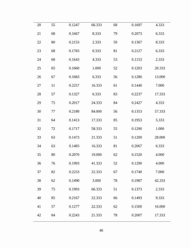
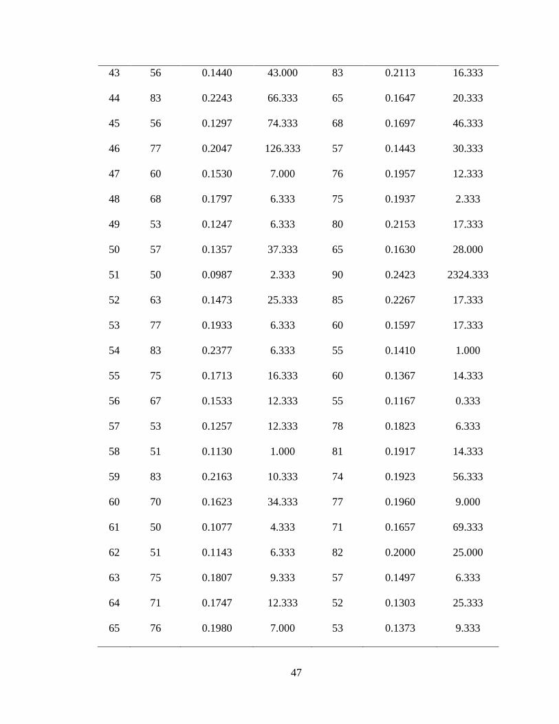
Appendix B. Mean and Variance of Width for Training Experiments

Exp.

No.

Current

1

(amps)

Mean

Width 1,2,3

(inches)

σ2

(inches *

(10^6))

Current

2

(amps)

Mean

Width 4,5,6

(inches)

σ2

(inches*

(10^6))

1 70 0.1507 4.333 50 0.0987 2.333

2 79 0.1853 9.333 63 0.1473 25.333

3 57 0.1267 9.333 77 0.1933 6.333

4 79 0.1993 9.333 83 0.2377 6.333

5 66 0.1447 0.333 75 0.1713 16.333

6 82 0.2090 9.000 67 0.1533 12.333

7 62 0.1503 4.333 53 0.1257 12.333

8 68 0.1603 2.333 51 0.1130 1.000

9 77 0.1967 25.333 83 0.2163 10.333

10 50 0.1153 20.333 70 0.1623 34.333

11 85 0.2183 12.333 50 0.1077 4.333

12 78 0.1937 2.333 51 0.1143 6.333

13 54 0.1157 16.333 75 0.1807 9.333

14 59 0.1420 12.000 71 0.1747 12.333

15 68 0.1660 21.000 76 0.1980 7.000

16 56 0.1340 16.000 75 0.1950 31.000

17 69 0.1649 6.253 50 0.1247 6.333

18 73 0.1750 31.000 68 0.1687 22.333

19 65 0.1570 39.000 76 0.1990 63.000

46

20 55 0.1247 66.333 68 0.1697 4.333

21 68 0.1667 8.333 79 0.2073 6.333

22 80 0.2153 2.333 59 0.1367 8.333

23 68 0.1783 0.333 81 0.2127 6.333

24 68 0.1643 4.333 53 0.1153 2.333

25 65 0.1660 1.000 52 0.1203 20.333

26 67 0.1683 6.333 56 0.1280 13.000

27 51 0.2257 16.333 61 0.1440 7.000

28 57 0.1327 6.333 83 0.2237 17.333

29 75 0.2017 24.333 84 0.2427 4.333

30 77 0.2180 84.000 56 0.1353 57.333

31 64 0.1413 17.333 85 0.1953 5.333

32 72 0.1717 58.333 55 0.1290 1.000

33 63 0.1473 21.333 51 0.1200 28.000

34 63 0.1483 16.333 81 0.2067 6.333

35 80 0.2070 19.000 62 0.1520 4.000

36 76 0.1993 41.333 52 0.1290 4.000

37 82 0.2233 22.333 67 0.1740 7.000

38 62 0.1490 3.000 78 0.1987 42.333

39 75 0.1993 66.333 51 0.1373 2.333

40 85 0.2167 22.333 66 0.1493 9.333

41 57 0.1277 22.333 62 0.1500 16.000

42 84 0.2243 21.333 78 0.2007 17.333

47

43 56 0.1440 43.000 83 0.2113 16.333

44 83 0.2243 66.333 65 0.1647 20.333

45 56 0.1297 74.333 68 0.1697 46.333

46 77 0.2047 126.333 57 0.1443 30.333

47 60 0.1530 7.000 76 0.1957 12.333

48 68 0.1797 6.333 75 0.1937 2.333

49 53 0.1247 6.333 80 0.2153 17.333

50 57 0.1357 37.333 65 0.1630 28.000

51 50 0.0987 2.333 90 0.2423 2324.333

52 63 0.1473 25.333 85 0.2267 17.333

53 77 0.1933 6.333 60 0.1597 17.333

54 83 0.2377 6.333 55 0.1410 1.000

55 75 0.1713 16.333 60 0.1367 14.333

56 67 0.1533 12.333 55 0.1167 0.333

57 53 0.1257 12.333 78 0.1823 6.333

58 51 0.1130 1.000 81 0.1917 14.333

59 83 0.2163 10.333 74 0.1923 56.333

60 70 0.1623 34.333 77 0.1960 9.000

61 50 0.1077 4.333 71 0.1657 69.333

62 51 0.1143 6.333 82 0.2000 25.000

63 75 0.1807 9.333 57 0.1497 6.333

64 71 0.1747 12.333 52 0.1303 25.333

65 76 0.1980 7.000 53 0.1373 9.333

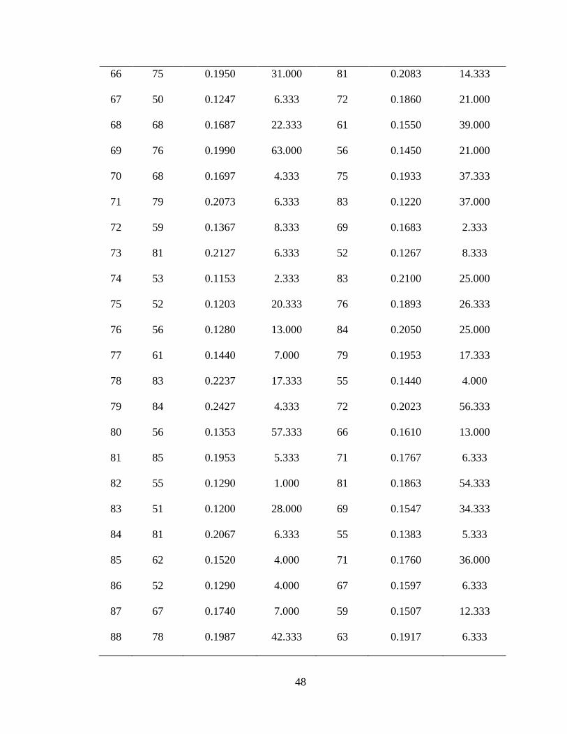
48

66 75 0.1950 31.000 81 0.2083 14.333

67 50 0.1247 6.333 72 0.1860 21.000

68 68 0.1687 22.333 61 0.1550 39.000

69 76 0.1990 63.000 56 0.1450 21.000

70 68 0.1697 4.333 75 0.1933 37.333

71 79 0.2073 6.333 83 0.1220 37.000

72 59 0.1367 8.333 69 0.1683 2.333

73 81 0.2127 6.333 52 0.1267 8.333

74 53 0.1153 2.333 83 0.2100 25.000

75 52 0.1203 20.333 76 0.1893 26.333

76 56 0.1280 13.000 84 0.2050 25.000

77 61 0.1440 7.000 79 0.1953 17.333

78 83 0.2237 17.333 55 0.1440 4.000

79 84 0.2427 4.333 72 0.2023 56.333

80 56 0.1353 57.333 66 0.1610 13.000

81 85 0.1953 5.333 71 0.1767 6.333

82 55 0.1290 1.000 81 0.1863 54.333

83 51 0.1200 28.000 69 0.1547 34.333

84 81 0.2067 6.333 55 0.1383 5.333

85 62 0.1520 4.000 71 0.1760 36.000

86 52 0.1290 4.000 67 0.1597 6.333

87 67 0.1740 7.000 59 0.1507 12.333

88 78 0.1987 42.333 63 0.1917 6.333

49

89 51 0.1373 2.333 69 0.1803 2.333

90 66 0.1493 9.333 80 0.1893 30.333

91 62 0.1500 16.000 55 0.1327 36.333

92 78 0.2007 17.333 60 0.1483 4.333

93 83 0.2113 16.333 71 0.1943 30.333

94 65 0.1647 20.333 77 0.2017 12.333

95 68 0.1697 46.333 81 0.2033 9.333

96 57 0.1443 30.333 70 0.1760 16.000

97 76 0.1957 12.333 71 0.1877 6.333

98 75 0.1937 2.333 85 0.2153 12.333

99 80 0.2153 17.333 50 0.1257 30.333

100 65 0.1630 28.000 51 0.1237 6.333

v1 56 0.1400 400.000 73 0.1857 1.333

v2 81 0.2407 12.333 64 0.1607 8.333

v3 78 0.2320 4.000 63 0.1643 0.333

v4 83 0.2443 5.333 58 0.1450 1.000

v5 68 0.1800 16.000 52 0.1200 4.000

50

Appendix C. Current & Width of Validation Experiments

Exp.

No.

Current 1

(amps)

Width 1

(inches)

Width 2

(inches)

Width 3

(inches)

Current 2

(amps)

Width 3

(inches)

Width 4

(inches)

Width 5

(inches)

v1 56 0.1600 0.1400 0.1200 73 0.1850 0.1870 0.1850

v2 81 0.2440 0.2370 0.2410 64 0.1640 0.1590 0.1590

v3 78 0.2300 0.2320 0.2340 63 0.1640 0.1650 0.1640

v4 83 0.2430 0.2470 0.2430 58 0.1450 0.1460 0.1440

v5 68 0.1800 0.1760 0.1840 52 0.1200 0.1220 0.1180

Appendix D. Mean & Variance of Width for Validation Experiments

Exp.

No.

Current

1

(amps)

Mean

Width 1,2,3

(inches)

σ2

(inches *

(10^6))

Current

2

(amps)

Mean

Width 4,5,6

(inches)

σ2

(inches*

(10^6))

v1 56 0.1400 400.000 73 0.1857 1.333

v2 81 0.2407 12.333 64 0.1607 8.333

v3 78 0.2320 4.000 63 0.1643 0.333

v4 83 0.2443 5.333 58 0.1450 1.000

v5 68 0.1800 16.000 52 0.1200 4.000

51

LITERATURE CITED

ABB. (2017). IRB 140 Industrial Robot [Technical Data Sheet pdf]. Retrieved from

http://new.abb.com/products/robotics/industrial-robots/irb-140

Alpaydin, E. (2014) Introduction to machine learning. Cambridge, MA: The MIT Press.

Baskaro, A., Tandian, R., Haikal, Edyanto, A., & Saragih, A. (2016). Automatic

Tungsten Inert Gas Welding Using Machine Vision and Neural Network on

Material SS304. International Conference on Advanced Computer Science and

Information Systems (ICACSIS), pp. 427-432.

CK Worldwide. (2017). Technical Guide Specifications for TIG Welding. [pdf

document]. Retrieved from

http://www.ckworldwide.com/Form%20116%20%20Technical%20Guide.pdf

Dong, H., Huff, S., Cong, M., Zhang, Y., Chen, H. (2016). Backside Weld Bead Shape

Modeling using Support Vector Machine (Unpublished report). Texas State

University, San Marcos, TX.

Dong, H., Cong*, M., Liu, Y., Zhang, Y., Chen, H. (2016) Predicting Characteristic

Performance for Arc Welding Process. IEEE International Conference on Cyber

Technology in Automation, Control, and Intelligent Systems (CYBER), pp 7-12.

Dong, H., Cong*, M., Zhang, Y., Liu, Y., Chen, H. (2017) IEEE International

Conference on Robotics Automation (ICRA), pp 1794-1799.

International Federation of Robotics. (2016). Industrial Robots 2016 [pdf document].

Retrieved from

https://ifr.org/img/office/Industrial_Robots_2016_Chapter_1_2.pdf

52

International Federation of Robotics. (2017). Executive Summary World Robotics 2017

Industrial Robots. [pdf document] Retrieved from

https://ifr.org/downloads/press/Executive_Summary_WR_2017_Industrial_Robot

s.pdf

Industrial robot. (2016). International Organization for Standardization online. ISO

8373:2012(en). Retrieved from https://www.iso.org/obp/ui/#iso:std:iso:8373:ed-

2:v1:en

Kaplan, J. (2016) Artificial intelligence: What Everyone Needs to Know. New York, NY:

Oxford University Press.

Keshmiri, S., Zheng, X., Feng, L., Pang, C., & Chew, C. (2015). Application of Deep

Neural Network in Estimation of the Weld Bead Parameters. IEEE/RSJ

International Conference on Intelligent Robots and Systems (IROS), pp. 3518-

3523.

Lee, Jaeyoung. (2007). Introduction to Offshore Pipelines & Risers [pdf document].

Retrieved from https://www.scribd.com/doc/238620580/Introduction-to-Offshore-

Pipelines-Risers-Jaeyoung-Lee.

Li, W., Gao, K., Wu, J., Hu, T., Wang, J. (2014). SVM-based information fusion for weld

deviation extraction and weld groove state identification in rotating arc narrow

gap MAG welding. The International Journal of Advanced Manufacturing

Technology, vol. 74, pp. 1355-1364.

Liu, Y.K., Zhang, W.J., & Zhang, Y. M. (2013). Neuro-fuzzy based human intelligence

modeling and robust control in Gas Tungsten Arc Welding Process. American

Control Conference (ACC), pp. 5631-5636.

53

Liu, Y.K., & Zhang, Y.M. (2014). Model-Based Predictive Control of Weld Penetration

in Gas Tungsten Arc Welding. IEEE Transactions on Control Systems

Technology, vol. 22, no. 3, pp. 955-966.

Liu, Y.K., Zhang, W.J., & Zhang, Y.M. (2015). Dynamic Neuro-Fuzzy-Based Human

Intelligence Modeling and Control in GTAW. IEEE Transactions on Automation

Science and Engineering, vol. 12, no. 1, pp. 324-335.

Patel, R. B., & Patel, N. S. (2014). A Review of Parametric Optimization of Tig Welding.

International Journal of Computational Engineering Research, 04, pp 27-31.

Rasmussen, C. E., Nickisch, H. (2017). Code from the Rasmussen and Williams:

Gaussian Process for Machine Learning book [Software]. Available from

http://www.gaussianprocess.org/gpml/code/matlab/doc/index.html

Russel, S. J., Norvig, P. (1995) Artificial Intelligence: A Modern Approach. Upper

Saddle River, NJ: Prentice Hall Publishing.

Snelson, E. (2006) Tutorial: Gaussian process models for machine learning [pdf

document]. Retrieved from http://mlg.eng.cam.ac.uk/tutorials/06/es.pdf

Sterling, D., Sterling, T., Zhang, Y., Chen, H. (2015). Welding Parameter Optimization

Based on Process Regression Bayesian Optimization Algorithm. IEEE

International Conference on Automation Science and Engineering (CASE), pp.

1490-1496.

Vinas, J., Cabrera, R., Juarez, I. (2016). On-line learning of welding bead geometry in

industrial robots. International Journal of Advanced Manufacturing Technology,

vol. 83, pp. 217-231.

54

Wallen, Johanna. (2008, May 8). The history of the industrial robot. Technical report

from Automatic Control at Linkopings universitet, LiTH-ISY-R-2853, 6-10.

Retrieved from

http://liu.divaportal.org/smash/get/diva2:316930/FULLTEXT01.pdf

Wang , S., Chaovalitwongse, W., & Babuska, R (2012). Machine learning algorithms in

bipedal robot control. IEEE Transactions on Systems Man and Cybernetics Part

C: Applications and Reviews, vol. 42, no. 5, pp. 728-743.

Wang, X., Li, R. (2014). Intelligent modelling of back-side weld bead geometry using

weld pool surface characteristic parameters. Journal of Intelligent Manufacturing,

vol. 25, no. 6, pp. 1301-1313.

Wang, X., Liu, Y.K., Zhang, W.J., & Zhang, Y. M. (2012). Estimation of weld

penetration using parameterized three-dimensional weld pool surface in gas

tungsten arc welding. IEEE International Symposium on Industrial Electronics

(ISIE2012), pp. 835-840.

Zhang, W.J., & Zhang, Y. M. (2012). Modeling of Human Welder Response to 3D Weld

Pool Surface: Part I-Principles. Welding Journal 91(11): 310-s to 318-s.