Tidal Wetland Vegetation in the San Francisco Bay Estuary: Modeling Species Distributions with Sea-Level Rise

By

Lisa Marie Schile

A dissertation submitted in partial satisfaction of the

requirements for the degree of

Doctor of Philosophy

in

Environmental Science, Policy, and Management

in the

Graduate Division

of the

University of California, Berkeley

Committee in Charge:

Professor Maggi Kelly, Chair Professor Katharine Suding

Professor Wayne Sousa

Fall 2012

Tidal Wetland Vegetation in the San Francisco Bay Estuary: Modeling Species Distributions with Sea-Level Rise

Copyright © 2012

by

Lisa Marie Schile

1  

Abstract

Tidal Wetland Vegetation in the San Francisco Bay Estuary: Modeling Species Distributions with Sea-Level Rise

by

Lisa Marie Schile

Doctor of Philosophy in Environmental Science, Policy, and Management

University of California, Berkeley

Professor Maggi Kelly, Chair

Tidal wetland ecosystems are dynamic coastal habitats that, in California, often occur at the complex nexus of aquatic environments, diked and leveed baylands, and modified upland habitat. Because of their prime coastal location and rich peat soil, many wetlands have been reduced, degraded, and/or destroyed, and yet their important role in carbon sequestration, nutrient and sediment filtering, flood control, and as habitat requires us to further research, conserve, and examine their sustainability, particularly in light of predicted climate change. Predictions of regional climate change effects for the San Francisco Bay Estuary present a future with reduced summer freshwater input and increased sea levels, resulting in higher estuarine salinities throughout the growing season, increased saline influence in brackish and freshwater marshes, and increased depth and duration of inundation. Experimentally testing, monitoring across scales, and spatially modeling the responses of dominant wetland vegetation to the substantial predicted climate change effects are among the critical threads of knowledge needed to understand how this estuary and others along the Pacific coast might respond to significant changes in physical drivers and community interactions. My dissertation research focused on possibilities for wetland resilience in a changing climate in the San Francisco Bay Estuary across scales and using a suite of methodologies. Tidal wetland resilience to predicted sea-level rise requires an understanding of both individual plant and community-level responses in addition their interactions with sediment supply and adjacent land uses. Through a large field experiment simulating sea-level rise, I found that wetland plants have a high tolerance for increases in inundation in the short term and that community interactions need to be incorporated into plant responses to increased sea-level rise. Scaling measurements of plant production up to the site level and across landscapes requires the integration of field measurements with remotely sensed measurements. Investigating remote sensing techniques of measuring carbon stock, I found that the presence of dense standing plant litter common in Pacific coast freshwater wetlands can hinder the ability to find a reliable way of measuring plant production remotely. Finally, I was able to successfully calibrate an ecogeomorphic mechanistic model for wetland accretion across four

2  

wetlands in the San Francisco Bay Estuary and examine potential wetland resiliency under a range of sea-level rise scenarios. At sea-level rise rates 100 cm/century and lower, wetlands remained vegetated. Once sea levels rise above 100 cm, marshes begin to lose ability to maintain elevation, and the presence of adjacent upland habitat becomes increasingly important for marsh migration. Results from this study emphasize that the wetland landscape in the bay is threatened with rising sea levels, and there are a limited number of wetlands that will be able to migrate to higher ground as sea levels rise. Despite these challenges, my dissertation presents a robust and new understanding of how tidal wetlands might respond to predicted climate change.  

i  

T A B L E O F C O N T E N T S

List of Figures .................................................................................................................. ii List of Tables ................................................................................................................... iv Acknowledgements ........................................................................................................ v Chapter One

Resiliency of tidal wetlands in San Francisco Bay Estuary to predicted climate change ............................................................................. 1

Chapter Two

Can community structure track sea-level rise? Stress and competitive controls in tidal wetlands ...................................................... 16

Chapter Three

Accounting for non-photosynthetic vegetation in remote sensing based estimates of carbon flux in wetlands ....................................... 35

Chapter Four

Modeling tidal wetland distribution with sea-level rise: evaluating the role of vegetation in marsh resiliency ................................................. 47

Chapter Five

Conclusion and directions for future research ............................................................ 75 References ...................................................................................................................... 79

ii  

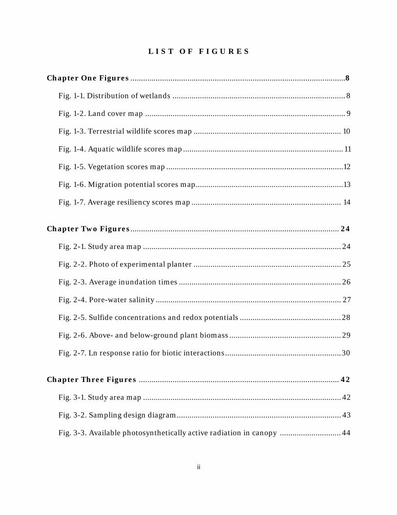
L I S T O F F I G U R E S Chapter One Figures ...................................................................................................... 8

Fig. 1-1. Distribution of wetlands .................................................................................. 8

Fig. 1-2. Land cover map ............................................................................................... 9

Fig. 1-3. Terrestrial wildlife scores map ...................................................................... 10

Fig. 1-4. Aquatic wildlife scores map ............................................................................ 11

Fig. 1-5. Vegetation scores map ....................................................................................12

Fig. 1-6. Migration potential scores map ...................................................................... 13

Fig. 1-7. Average resiliency scores map ....................................................................... 14

Chapter Two Figures ................................................................................................... 24

Fig. 2-1. Study area map .............................................................................................. 24

Fig. 2-2. Photo of experimental planter ...................................................................... 25

Fig. 2-3. Average inundation times ............................................................................. 26

Fig. 2-4. Pore-water salinity ........................................................................................ 27

Fig. 2-5. Sulfide concentrations and redox potentials ................................................ 28

Fig. 2-6. Above- and below-ground plant biomass ..................................................... 29

Fig. 2-7. Ln response ratio for biotic interactions ....................................................... 30

Chapter Three Figures ............................................................................................... 42

Fig. 3-1. Study area map .............................................................................................. 42

Fig. 3-2. Sampling design diagram .............................................................................. 43

Fig. 3-3. Available photosynthetically active radiation in canopy ............................. 44

iii  

Fig. 3-4. Relationship between photosynthetically active radiation and spectral indices .......................................................................................................................... 45 Fig. 3-5. Correlation matrices of photosynthetically active radiation and spectral indices .......................................................................................................................... 46

Chapter Four Figures ................................................................................................. 58

Fig. 4-1. Study area map and initial wetland habitat distributions ............................ 58

Fig. 4-2. Plant biomass along elevation gradient ........................................................ 59

Fig. 4-3. Histogram of plant biomass .......................................................................... 60

Fig. 4-4. Percent cover of habitat types with sea-level rise ......................................... 61

Fig. 4-5. Percent cover of habitat types with sea-level rise ........................................ 62

Fig. 4-6. Maps of habitat types with century sea-level rise at China Camp ................ 63

Fig. 4-7. Maps of habitat types with century sea-level rise at Coon Island ................ 64

Fig. 4-8. Maps of habitat types with century sea-level rise at Rush Ranch ................ 65

Fig. 4-9. Maps of habitat types with century sea-level rise at Browns Island ............ 66

Fig. 4-10. Model calibration with soil cores accretion rates ....................................... 67

Fig. 4-11. Percent cover of habitat types with 24 cm/ century sea-level rise ............. 68

Fig. 4-12. Maps of habitat types with century sea-level rise at Rush Ranch .............. 69

iv  

L I S T O F T A B L E S

Chapter One Tables ...................................................................................................... 15

Table 1-1. Ranks of land cover types ............................................................................. 15

Chapter Two Tables ...................................................................................................... 31

Table 2-1. Tidal metrics ................................................................................................ 31

Table 2-2. Statistical results of physical processes analyses ...................................... 32

Table 2-3. Statistical results of biomass analyses ....................................................... 33

Table 2-4. Statistical results of biotic interaction analyses ......................................... 34

Chapter Four Tables .................................................................................................... 70

Table 4-1. Study site characteristics ............................................................................ 70

Table 4-2. Area of habitat types .................................................................................... 71

Table 4-3. Model inputs ............................................................................................... 72

Table 4-4. Relative elevation key for habitat types ..................................................... 73

Table 4-5. Model calibration results with soil core accretion rates ........................... 74

v  

A C K N O W L E D G E M E N T S

I would like to truly thank my advisor, Maggi Kelly, and committee members, Wayne Sousa and Katharine Suding, for their thoughtful guidance and support throughout my tenure as a graduate student. I am now a stronger scientist, more skilled researcher, and immensely better public speaker. My research was funded under California Bay-Delta Authority Agreement No. U-04-SC-005, CALFED Science Program Grant #1037, and the NASA New Investigator Program in Earth Sciences Grant Number # NNH10A086I. This work was conducted in part while I was a member of the working group on “Tidal Wetland Carbon Sequestration and Greenhouse Gas Emissions Model” at the National Center for Ecological Analysis and Synthesis (NCEAS). Without permission from the California Department of Fish and Wildlife, the East Bay Regional Park District, the Solano Land Trust, and the San Francisco Bay National Estuarine Research Reserve System, I would have been unable to conduct my field research. The statements, findings, conclusions and recommendations in this dissertation are mine and do not necessarily reflect the views of the aforementioned organizations. Any use of trade, firm, or product names is for descriptive purposes only and does not imply endorsement by the U.S. Government. This dissertation would not have been possible without the support of many amazing people. I truly appreciate the logistical help from James Morris, V. Thomas Parker, Kristin Byrd, Diana Stralberg, and Lisamarie Windham-Myers. Your assistance and knowledge has strengthened the quality and breadth of my research. Ryan Halwachs, Eyvan Borgnis, Sophie Kolding, and Andrea Torres were instrumental in helping with field work. Brooke Buchanan, Melissa Waters, Daniel Markovski, Diana Benner, Marilyn Latta, the Santa Cruz crew, Sarah Wagner, Ed Cissel, Brian Wickcliff, and Theresa Engle kept me grounded both during and after work. I am forever thankful for all of the volunteers that helped pound over 150 meters of 2x4 off of the side of the boat and move 3 cubic meters of mud multiple times. I particularly want to thank Nancy and Charles Schile; without their help, I would still be rinsing and sorting roots and rhizomes. Finally, I want to extend a special thank you to John Callaway for his constant encouragement, guidance, and field support. I could not have done this research without you.

1  

C H A P T E R O N E

Resiliency of tidal wetlands in San Francisco Bay Estuary to predicted climate change

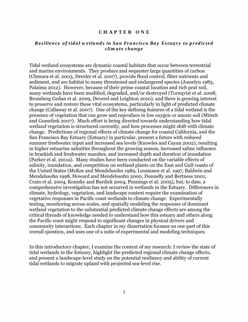
Tidal wetland ecosystems are dynamic coastal habitats that occur between terrestrial and marine environments. They produce and sequester large quantities of carbon (Chmura et al. 2003, Drexler et al. 2007), provide flood control, filter nutrients and sediment, and are habitat to many threatened and endangered species (Josselyn 1983, Palaima 2012). However, because of their prime coastal location and rich peat soil, many wetlands have been modified, degraded, and/or destroyed (Tornqvist et al. 2008, Bromberg Gedan et al. 2009, Deverel and Leighton 2010), and there is growing interest to preserve and restore these vital ecosystems, particularly in light of predicted climate change (Callaway et al. 2007). One of the key defining features of a tidal wetland is the presence of vegetation that can grow and reproduce in low oxygen or anoxic soil (Mitsch and Gosselink 2007). Much effort is being directed towards understanding how tidal wetland vegetation is structured currently, and how processes might shift with climate change. Predictions of regional effects of climate change for coastal California, and the San Francisco Bay Estuary (Estuary) in particular, present a future with reduced summer freshwater input and increased sea levels (Knowles and Cayan 2002), resulting in higher estuarine salinities throughout the growing season, increased saline influence in brackish and freshwater marshes, and increased depth and duration of inundation (Parker et al. 2011a). Many studies have been conducted on the variable effects of salinity, inundation, and competition on wetland plants on the East and Gulf coasts of the United States (McKee and Mendelssohn 1989, Lessmann et al. 1997, Baldwin and Mendelssohn 1998, Howard and Mendelssohn 2000, Donnelly and Bertness 2001, Crain et al. 2004, Konisky and Burdick 2004, Pennings et al. 2005), but, to date, a comprehensive investigation has not occurred in wetlands in the Estuary. Differences in climate, hydrology, vegetation, and landscape context require the examination of vegetative responses in Pacific coast wetlands to climate change. Experimentally testing, monitoring across scales, and spatially modeling the responses of dominant wetland vegetation to the substantial predicted climate change effects are among the critical threads of knowledge needed to understand how this estuary and others along the Pacific coast might respond to significant changes in physical drivers and community interactions. Each chapter in my dissertation focuses on one part of this overall question, and uses one of a suite of experimental and modeling techniques.

In this introductory chapter, I examine the context of my research: I review the state of tidal wetlands in the Estuary, highlight the predicted regional climate change effects, and present a landscape-level study on the potential resiliency and ability of current tidal wetlands to migrate upland with projected sea-level rise.

2  

Importance of Tidal Marshes of San Francisco Bay Estuary

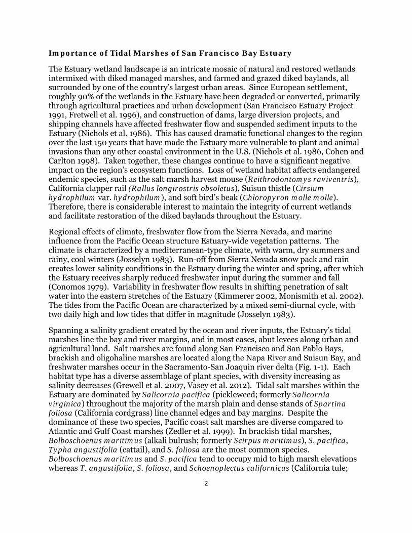
The Estuary wetland landscape is an intricate mosaic of natural and restored wetlands intermixed with diked managed marshes, and farmed and grazed diked baylands, all surrounded by one of the country’s largest urban areas. Since European settlement, roughly 90% of the wetlands in the Estuary have been degraded or converted, primarily through agricultural practices and urban development (San Francisco Estuary Project 1991, Fretwell et al. 1996), and construction of dams, large diversion projects, and shipping channels have affected freshwater flow and suspended sediment inputs to the Estuary (Nichols et al. 1986). This has caused dramatic functional changes to the region over the last 150 years that have made the Estuary more vulnerable to plant and animal invasions than any other coastal environment in the U.S. (Nichols et al. 1986, Cohen and Carlton 1998). Taken together, these changes continue to have a significant negative impact on the region’s ecosystem functions. Loss of wetland habitat affects endangered endemic species, such as the salt marsh harvest mouse (Reithrodontomys raviventris), California clapper rail (Rallus longirostris obsoletus), Suisun thistle (Cirsium hydrophilum var. hydrophilum), and soft bird’s beak (Chloropyron molle molle). Therefore, there is considerable interest to maintain the integrity of current wetlands and facilitate restoration of the diked baylands throughout the Estuary.

Regional effects of climate, freshwater flow from the Sierra Nevada, and marine influence from the Pacific Ocean structure Estuary-wide vegetation patterns. The climate is characterized by a mediterranean-type climate, with warm, dry summers and rainy, cool winters (Josselyn 1983). Run-off from Sierra Nevada snow pack and rain creates lower salinity conditions in the Estuary during the winter and spring, after which the Estuary receives sharply reduced freshwater input during the summer and fall (Conomos 1979). Variability in freshwater flow results in shifting penetration of salt water into the eastern stretches of the Estuary (Kimmerer 2002, Monismith et al. 2002). The tides from the Pacific Ocean are characterized by a mixed semi-diurnal cycle, with two daily high and low tides that differ in magnitude (Josselyn 1983).

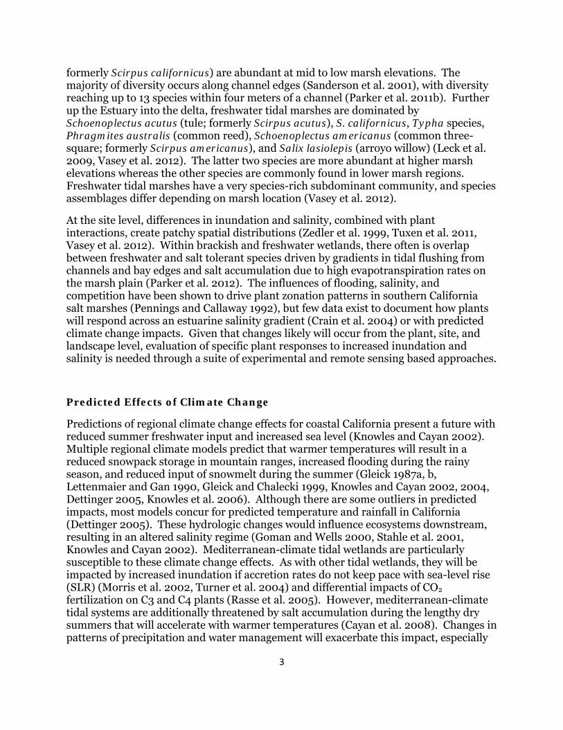
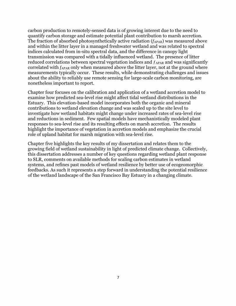
Spanning a salinity gradient created by the ocean and river inputs, the Estuary’s tidal marshes line the bay and river margins, and in most cases, abut levees along urban and agricultural land. Salt marshes are found along San Francisco and San Pablo Bays, brackish and oligohaline marshes are located along the Napa River and Suisun Bay, and freshwater marshes occur in the Sacramento-San Joaquin river delta (Fig. 1-1). Each habitat type has a diverse assemblage of plant species, with diversity increasing as salinity decreases (Grewell et al. 2007, Vasey et al. 2012). Tidal salt marshes within the Estuary are dominated by Salicornia pacifica (pickleweed; formerly Salicornia virginica) throughout the majority of the marsh plain and dense stands of Spartina foliosa (California cordgrass) line channel edges and bay margins. Despite the dominance of these two species, Pacific coast salt marshes are diverse compared to Atlantic and Gulf Coast marshes (Zedler et al. 1999). In brackish tidal marshes, Bolboschoenus maritimus (alkali bulrush; formerly Scirpus maritimus), S. pacifica, Typha angustifolia (cattail), and S. foliosa are the most common species. Bolboschoenus maritimus and S. pacifica tend to occupy mid to high marsh elevations whereas T. angustifolia, S. foliosa, and Schoenoplectus californicus (California tule;

3  

formerly Scirpus californicus) are abundant at mid to low marsh elevations. The majority of diversity occurs along channel edges (Sanderson et al. 2001), with diversity reaching up to 13 species within four meters of a channel (Parker et al. 2011b). Further up the Estuary into the delta, freshwater tidal marshes are dominated by Schoenoplectus acutus (tule; formerly Scirpus acutus), S. californicus, Typha species, Phragmites australis (common reed), Schoenoplectus americanus (common three-square; formerly Scirpus americanus), and Salix lasiolepis (arroyo willow) (Leck et al. 2009, Vasey et al. 2012). The latter two species are more abundant at higher marsh elevations whereas the other species are commonly found in lower marsh regions. Freshwater tidal marshes have a very species-rich subdominant community, and species assemblages differ depending on marsh location (Vasey et al. 2012).

At the site level, differences in inundation and salinity, combined with plant interactions, create patchy spatial distributions (Zedler et al. 1999, Tuxen et al. 2011, Vasey et al. 2012). Within brackish and freshwater wetlands, there often is overlap between freshwater and salt tolerant species driven by gradients in tidal flushing from channels and bay edges and salt accumulation due to high evapotranspiration rates on the marsh plain (Parker et al. 2012). The influences of flooding, salinity, and competition have been shown to drive plant zonation patterns in southern California salt marshes (Pennings and Callaway 1992), but few data exist to document how plants will respond across an estuarine salinity gradient (Crain et al. 2004) or with predicted climate change impacts. Given that changes likely will occur from the plant, site, and landscape level, evaluation of specific plant responses to increased inundation and salinity is needed through a suite of experimental and remote sensing based approaches.

Predicted Effects of Climate Change

Predictions of regional climate change effects for coastal California present a future with reduced summer freshwater input and increased sea level (Knowles and Cayan 2002). Multiple regional climate models predict that warmer temperatures will result in a reduced snowpack storage in mountain ranges, increased flooding during the rainy season, and reduced input of snowmelt during the summer (Gleick 1987a, b, Lettenmaier and Gan 1990, Gleick and Chalecki 1999, Knowles and Cayan 2002, 2004, Dettinger 2005, Knowles et al. 2006). Although there are some outliers in predicted impacts, most models concur for predicted temperature and rainfall in California (Dettinger 2005). These hydrologic changes would influence ecosystems downstream, resulting in an altered salinity regime (Goman and Wells 2000, Stahle et al. 2001, Knowles and Cayan 2002). Mediterranean-climate tidal wetlands are particularly susceptible to these climate change effects. As with other tidal wetlands, they will be impacted by increased inundation if accretion rates do not keep pace with sea-level rise (SLR) (Morris et al. 2002, Turner et al. 2004) and differential impacts of CO2 fertilization on C3 and C4 plants (Rasse et al. 2005). However, mediterranean-climate tidal systems are additionally threatened by salt accumulation during the lengthy dry summers that will accelerate with warmer temperatures (Cayan et al. 2008). Changes in patterns of precipitation and water management will exacerbate this impact, especially

4  

given the increased societal demands for water in a semi-arid climate (Cloern et al. 2011).

Sea levels are expected to rise as more snow and ice sheets melt and oceans thermally expand with predicted increases in temperature (Intergovernmental Panel on Climate Change 2007). Most tidal marshes accumulate 2-8 mm of sediment per year (Stevenson et al. 1986, Reed 1995, Callaway et al. 1996, Callaway et al. 2012), and this compensates for current (2-3 mm per year) increases in sea-level rise (SLR), compaction, and subsidence. However, SLR is projected to increase up to 100 cm over the next 100 years (Intergovernmental Panel on Climate Change 2007, National Research Council 2012), with some projections as high as 180 cm (Vermeer and Rahmstorf 2009). Tidal marshes will either maintain elevations through mineral and organic matter accretion, migrate inland to adjacent terrestrial areas, or face increased inundation (Donnelly and Bertness 2001, Morris et al. 2002). Substantial data from Louisiana, Chesapeake Bay, and modeling studies have shown that as increases in relative sea level get close to 10 to 12 mm/yr, most marshes cannot keep pace and vegetation eventually may be inundated and converted to open water/mudflats (Baumann et al. 1984, Kearney and Stevenson 1991, Boesch et al. 1994, Morris et al. 2002, Rasse et al. 2005, Stralberg et al. 2011).

Although it may be possible for marsh accretion in the San Francisco Bay to keep up with SLR (Orr et al. 2003, Callaway et al. 2012), studies have shown a decline in bay sediments over time due to dams and river diversions (Foxgrover et al. 2004, Schoellhamer 2011) and predict further declines (Cloern et al. 2011), and future large-scale tidal marsh restoration projects may further deplete existing bay sediments. Increases in water salinity on the order of five to seven parts per thousand can result in a reduction in plant biomass and diversity, particularly in brackish and freshwater marshes (Parker et al. 2012, Vasey et al. 2012), which reduces the organic matter input available for wetland accretion. Furthermore, in the highly urbanized Estuary system, tidal wetlands are restricted in terms of adjacent terrestrial habitats for upslope migration in response to SLR. These factors present a complicated and uncertain future for the resiliency of tidal wetlands in the Estuary in the face of predicted sea-level rise rates up to 180 cm in the next century.

Wetland Landscape Context

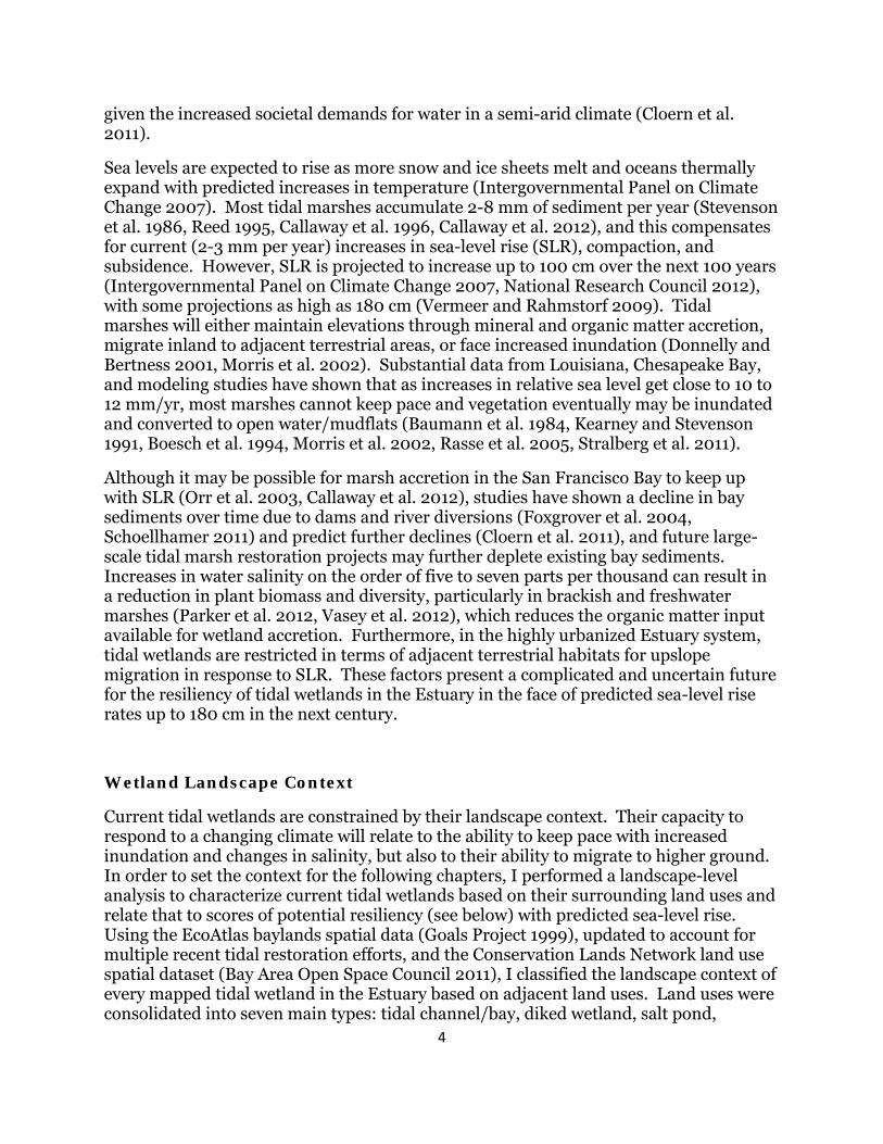
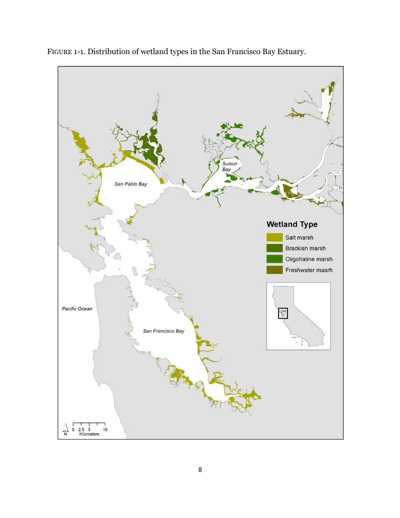
Current tidal wetlands are constrained by their landscape context. Their capacity to respond to a changing climate will relate to the ability to keep pace with increased inundation and changes in salinity, but also to their ability to migrate to higher ground. In order to set the context for the following chapters, I performed a landscape-level analysis to characterize current tidal wetlands based on their surrounding land uses and relate that to scores of potential resiliency (see below) with predicted sea-level rise. Using the EcoAtlas baylands spatial data (Goals Project 1999), updated to account for multiple recent tidal restoration efforts, and the Conservation Lands Network land use spatial dataset (Bay Area Open Space Council 2011), I classified the landscape context of every mapped tidal wetland in the Estuary based on adjacent land uses. Land uses were consolidated into seven main types: tidal channel/bay, diked wetland, salt pond,

5  

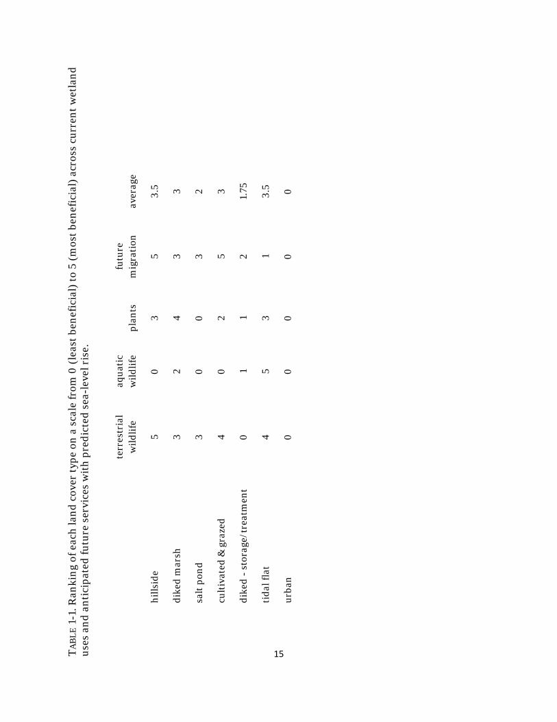
cultivated and/or grazed bayland, storage/treatment pond, hillside, and urban (Fig. 1-2). The diked wetland category encompassed managed marshes, muted marshes, diked wetlands, and managed diked wetlands. Cultivated and/or grazed baylands incorporated farmed, grazed, and filled baylands. The urban category included both urban and rural residential areas. Salt ponds are former tidal wetlands that have been diked and managed for salt production. Surrounding land use types for each wetland polygon were identified by creating a ten meter buffer around the wetland in ArcMap 10.0 (ESRI Inc. 2010), intersecting and then joining the buffer with surrounding landcover types; results were summarized for each wetland. Each land use type was scored on a scale of 0 (no benefit) to 5 (most benefit) based on ecosystem services for four metrics: current value for terrestrial wildlife (resident and breeding birds; mammals), aquatic wildlife, and vegetation, and future benefit for either direct marsh migration or availability after removing levees or if some other management modification occurred. An average resiliency score was also calculated. The five resiliency scores were applied to each tidal wetland depending on surrounding land use and average scores were used if multiple land uses occurred around a wetland. The scores for each metric were mapped at the Estuary-level.

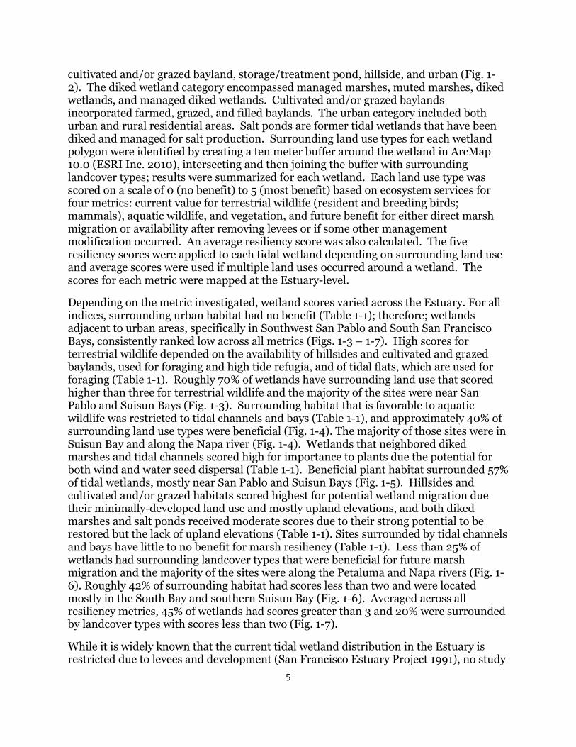
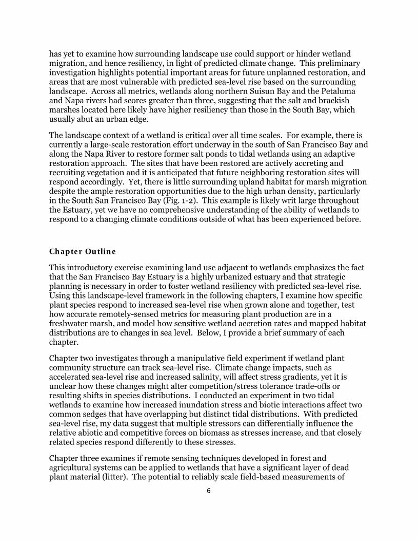
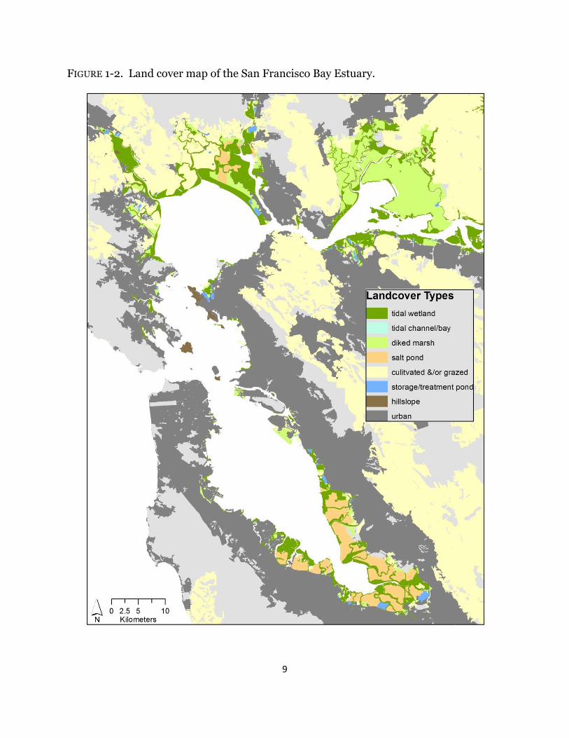
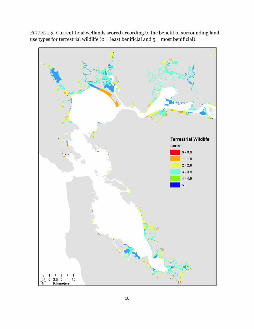
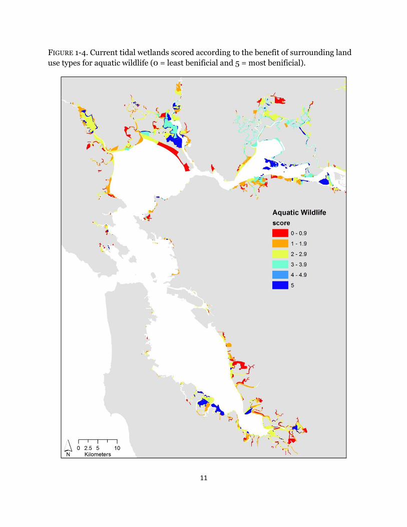
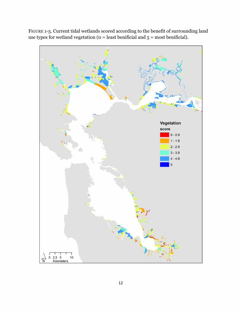
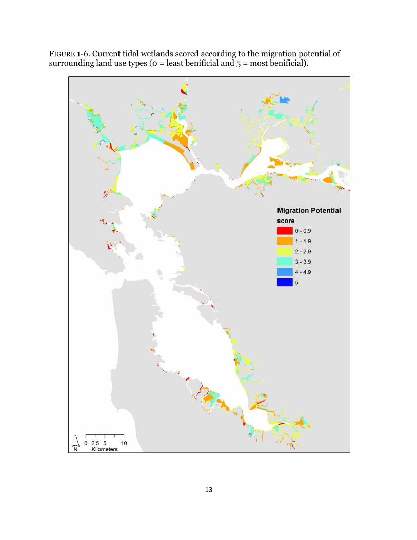
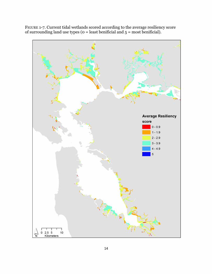
Depending on the metric investigated, wetland scores varied across the Estuary. For all indices, surrounding urban habitat had no benefit (Table 1-1); therefore; wetlands adjacent to urban areas, specifically in Southwest San Pablo and South San Francisco Bays, consistently ranked low across all metrics (Figs. 1-3 – 1-7). High scores for terrestrial wildlife depended on the availability of hillsides and cultivated and grazed baylands, used for foraging and high tide refugia, and of tidal flats, which are used for foraging (Table 1-1). Roughly 70% of wetlands have surrounding land use that scored higher than three for terrestrial wildlife and the majority of the sites were near San Pablo and Suisun Bays (Fig. 1-3). Surrounding habitat that is favorable to aquatic wildlife was restricted to tidal channels and bays (Table 1-1), and approximately 40% of surrounding land use types were beneficial (Fig. 1-4). The majority of those sites were in Suisun Bay and along the Napa river (Fig. 1-4). Wetlands that neighbored diked marshes and tidal channels scored high for importance to plants due the potential for both wind and water seed dispersal (Table 1-1). Beneficial plant habitat surrounded 57% of tidal wetlands, mostly near San Pablo and Suisun Bays (Fig. 1-5). Hillsides and cultivated and/or grazed habitats scored highest for potential wetland migration due their minimally-developed land use and mostly upland elevations, and both diked marshes and salt ponds received moderate scores due to their strong potential to be restored but the lack of upland elevations (Table 1-1). Sites surrounded by tidal channels and bays have little to no benefit for marsh resiliency (Table 1-1). Less than 25% of wetlands had surrounding landcover types that were beneficial for future marsh migration and the majority of the sites were along the Petaluma and Napa rivers (Fig. 1-6). Roughly 42% of surrounding habitat had scores less than two and were located mostly in the South Bay and southern Suisun Bay (Fig. 1-6). Averaged across all resiliency metrics, 45% of wetlands had scores greater than 3 and 20% were surrounded by landcover types with scores less than two (Fig. 1-7).

While it is widely known that the current tidal wetland distribution in the Estuary is restricted due to levees and development (San Francisco Estuary Project 1991), no study

6  

has yet to examine how surrounding landscape use could support or hinder wetland migration, and hence resiliency, in light of predicted climate change. This preliminary investigation highlights potential important areas for future unplanned restoration, and areas that are most vulnerable with predicted sea-level rise based on the surrounding landscape. Across all metrics, wetlands along northern Suisun Bay and the Petaluma and Napa rivers had scores greater than three, suggesting that the salt and brackish marshes located here likely have higher resiliency than those in the South Bay, which usually abut an urban edge.

The landscape context of a wetland is critical over all time scales. For example, there is currently a large-scale restoration effort underway in the south of San Francisco Bay and along the Napa River to restore former salt ponds to tidal wetlands using an adaptive restoration approach. The sites that have been restored are actively accreting and recruiting vegetation and it is anticipated that future neighboring restoration sites will respond accordingly. Yet, there is little surrounding upland habitat for marsh migration despite the ample restoration opportunities due to the high urban density, particularly in the South San Francisco Bay (Fig. 1-2). This example is likely writ large throughout the Estuary, yet we have no comprehensive understanding of the ability of wetlands to respond to a changing climate conditions outside of what has been experienced before.

Chapter Outline

This introductory exercise examining land use adjacent to wetlands emphasizes the fact that the San Francisco Bay Estuary is a highly urbanized estuary and that strategic planning is necessary in order to foster wetland resiliency with predicted sea-level rise. Using this landscape-level framework in the following chapters, I examine how specific plant species respond to increased sea-level rise when grown alone and together, test how accurate remotely-sensed metrics for measuring plant production are in a freshwater marsh, and model how sensitive wetland accretion rates and mapped habitat distributions are to changes in sea level. Below, I provide a brief summary of each chapter.

Chapter two investigates through a manipulative field experiment if wetland plant community structure can track sea-level rise. Climate change impacts, such as accelerated sea-level rise and increased salinity, will affect stress gradients, yet it is unclear how these changes might alter competition/stress tolerance trade-offs or resulting shifts in species distributions. I conducted an experiment in two tidal wetlands to examine how increased inundation stress and biotic interactions affect two common sedges that have overlapping but distinct tidal distributions. With predicted sea-level rise, my data suggest that multiple stressors can differentially influence the relative abiotic and competitive forces on biomass as stresses increase, and that closely related species respond differently to these stresses.

Chapter three examines if remote sensing techniques developed in forest and agricultural systems can be applied to wetlands that have a significant layer of dead plant material (litter). The potential to reliably scale field-based measurements of

7  

carbon production to remotely-sensed data is of growing interest due to the need to quantify carbon storage and estimate potential plant contribution to marsh accretion. The fraction of absorbed photosynthetically active radiation (fAPAR) was measured above and within the litter layer in a managed freshwater wetland and was related to spectral indices calculated from in-situ spectral data, and the difference in canopy light transmission was compared with a tidally influenced wetland. The presence of litter reduced correlations between spectral vegetation indices and ƒAPAR and was significantly correlated with fAPAR only when measured above the litter layer, not at the ground where measurements typically occur. These results, while demonstrating challenges and issues about the ability to reliably use remote sensing for large-scale carbon monitoring, are nonetheless important to report.

Chapter four focuses on the calibration and application of a wetland accretion model to examine how predicted sea-level rise might affect tidal wetland distributions in the Estuary. This elevation-based model incorporates both the organic and mineral contributions to wetland elevation change and was scaled up to the site level to investigate how wetland habitats might change under increased rates of sea-level rise and reductions in sediment. Few spatial models have mechanistically modeled plant responses to sea-level rise and its resulting effects on marsh accretion. The results highlight the importance of vegetation in accretion models and emphasize the crucial role of upland habitat for marsh migration with sea-level rise.

Chapter five highlights the key results of my dissertation and relates them to the growing field of wetland sustainability in light of predicted climate change. Collectively, this dissertation addresses a number of key questions regarding wetland plant response to SLR, comments on available methods for scaling carbon estimates in wetland systems, and refines past models of wetland resilience by better use of ecogeomorphic feedbacks. As such it represents a step forward in understanding the potential resilience of the wetland landscape of the San Francisco Bay Estuary in a changing climate.

8  

FIGURE 1-1. Distribution of wetland types in the San Francisco Bay Estuary.

9  

FIGURE 1-2. Land cover map of the San Francisco Bay Estuary.

10  

FIGURE 1-3. Current tidal wetlands scored according to the benefit of surrounding land use types for terrestrial wildlife (0 = least benificial and 5 = most benificial).

11  

FIGURE 1-4. Current tidal wetlands scored according to the benefit of surrounding land use types for aquatic wildlife (0 = least benificial and 5 = most benificial).

12  

FIGURE 1-5. Current tidal wetlands scored according to the benefit of surrounding land use types for wetland vegetation (0 = least benificial and 5 = most benificial).

13  

FIGURE 1-6. Current tidal wetlands scored according to the migration potential of surrounding land use types (0 = least benificial and 5 = most benificial).

14  

FIGURE 1-7. Current tidal wetlands scored according to the average resiliency score of surrounding land use types (0 = least benificial and 5 = most benificial).

     15 TA

BL

E 1

-1. R

anki

ng

of e

ach

lan

d c

over

typ

e on

a s

cale

fro

m 0

(le

ast

ben

efic

ial)

to

5 (m

ost

ben

efic

ial)

acr

oss

curr

ent

wet

lan

d

use

s an

d a

nti

cip

ated

fu

ture

ser

vice

s w

ith

pre

dic

ted

sea

-lev

el r

ise.

terr

estr

ial

wil

dli

fe

aqu

atic

w

ild

life

p

lan

ts

futu

re

mig

rati

on

aver

age

hil

lsid

e 5

0

3 5

3.5

dik

ed m

arsh

3

2 4

3

3

salt

pon

d

3 0

0

3

2

cult

ivat

ed &

gra

zed

4

0

2

5 3

dik

ed -

sto

rage

/tre

atm

ent

0

1 1

2 1.

75

tid

al f

lat

4

5 3

1 3.

5

urb

an

0

0

0

0

0

 

 

16  

C H A P T E R T W O

Can community structure track sea-level rise? Stress and competitive controls in tidal wetlands

The relative importance of abiotic and biotic factors often shifts along stress gradients, with biotic interactions changing from competition to facilitation with increasing physiological stress. Climate change impacts, such as accelerated sea-level rise and increased salinity, will affect stress gradients, yet it is unclear how these changes might alter competition/stress tolerance trade-offs or resulting shifts in species distributions. I conducted an experiment in two tidal wetlands to examine how increased inundation stress and biotic interactions affect two common sedges, Schoenoplectus acutus and Schoenoplectus americanus, that have overlapping but distinct tidal distributions. As hypothesized, S. acutus, which occupies low marsh habitats, best tolerated inundation stress, regardless of neighbors. Contrary to predictions, facilitation of either species was not documented with increased inundation stress. At the fresher site, S. americanus was competitively superior to S. acutus at the highest elevation. Schoenoplectus americanus never out-competed S. acutus at the saltier site and had reduced biomass with competition at every elevation. The competitive superiority of the stress tolerator (S. acutus) at the saltier site was not predicted by the stress/competition trade-off model and points to important synergies between multiple stressors. With predicted sea-level rise, my data suggest that multiple stressors can differentially influence the relative abiotic and competitive forces on biomass as stresses increase. Introduction The role of abiotic and biotic stresses on structuring plant communities and distributions has been widely examined (Pennings and Callaway 1992, Greiner La Peyre et al. 2001, Hillyer and Silman 2010) and often is complex (Guo and Pennings 2012). In many ecosystems, abiotic stresses and biotic interactions bound the lower and upper distributions, respectively, along gradients (Connell 1961, Crain et al. 2004). The effect of biotic interactions has been demonstrated to shift from competition to facilitation as abiotic stress increases (Bertness and Callaway 1994) and can vary depending on the nature of the abiotic stress and species involved (Maestre et al. 2009). Little is known, however, about the role of accelerated climate change in the context of trade-offs between stress tolerance, competition, and facilitation (Gilman et al. 2010, Maestre et al. 2010, Adler et al. 2012). Changes in climate are predicted to influence plant communities through shifts in temperature, carbon dioxide concentrations, sea level, precipitation, and nitrogen, among others, which are apparent already through changes in distribution, productivity, and phenology (Parmesan and Yohe 2003, Zavaleta et al. 2003, Jump and Peñuelas 2005). With predicted accelerated climate change, the influence and impact of abiotic stress, competition, and facilitation are likely to shift (Brooker 1996, Suttle et al. 2007), yet many uncertainties remain regarding how species distribution and abundance will be affected.

 

17  

Estuaries are a model habitat to study species interactions along stress gradients due to the clear identification of dominant stressors present (Pennings and Callaway 1992), the compact nature of the gradient, and the significant negative effects of predicted climate change (Donnelly and Bertness 2001). Sea levels are predicted to rise between 0.4 and 1.8 m by 2100 (Vermeer and Rahmstorf 2009), and concurrent with this rise are increases in salinity (Cloern et al. 2011). Tidal wetlands are a key ecosystem within coastal environments that produce and sequester significant quantities of carbon (Bridgham et al. 2006). Marshes respond to changes in sea level through accretion by mineral and organic inputs and by migrating up or down-slope (Morris et al. 2002). Therefore, understanding how biotic and abiotic factors interact to affect both above- and below-ground biomass and species distributions is key to predicting how these systems will fare with accelerated rates of sea-level rise. While greenhouse experiments provide essential information on plant growth under controlled conditions (Greiner La Peyre et al. 2001, Cherry et al. 2009), here I test the effect of increased abiotic stresses and biotic interactions on plant growth under field conditions, which often are difficult to realistically simulate. I chose two cosmopolitan wetland sedge species, Schoenoplectus acutus (Muhl. ex Bigelow) Á. Löve & D. Löve var. occidentalis (S. Watson) S.G. Sm. and Schoenoplectus americanus (Pers.) Volkart ex Schinz & R. Keller, that have adjacent, slightly overlapping tidal distributions in the San Francisco Bay estuary, California, USA, and different rhizome and stem morphology. A common mid and high species marsh, S. americanus has been studied widely under a variety of climate change and competition scenarios along the Atlantic coast and Gulf of Mexico, including flooding, increased carbon dioxide concentrations, and nutrient addition (Broome et al. 1995, Erickson et al. 2007, Langley et al. 2009, Kirwan and Guntensbergen 2012); however, field experiments have not specifically addressed how sea-level rise affects abiotic and biotic interactions. Little is known about the responses of S. acutus, which is characteristic of lower marsh zones, to increased inundation and neighbor interactions in tidal systems. In this paper, I investigated the individual and combined effects of increased inundation and biotic interactions on above- and below-ground biomass of S. acutus and S. americanus at two tidal wetlands that differ slightly in salinity. I grew the plants at elevations lower than current distributions to simulate sea-level rise. Based on current marsh distributions, I hypothesized that: 1) S. acutus would have better performance than S. americanus under conditions of increased inundation without competition (better stress tolerator); 2) S. americanus would have a competitive advantage at higher elevations due to the clumping rhizome growth pattern, and dominance throughout the marsh plain (better competitor); and 3) S. acutus would facilitate the growth of its congener at the lowest elevations (increased facilitation with stress). I employed a unique experimental design that allowed us to test these hypotheses under field conditions across existing elevations and those not currently found within marshes to reflect potential future conditions.

 

18  

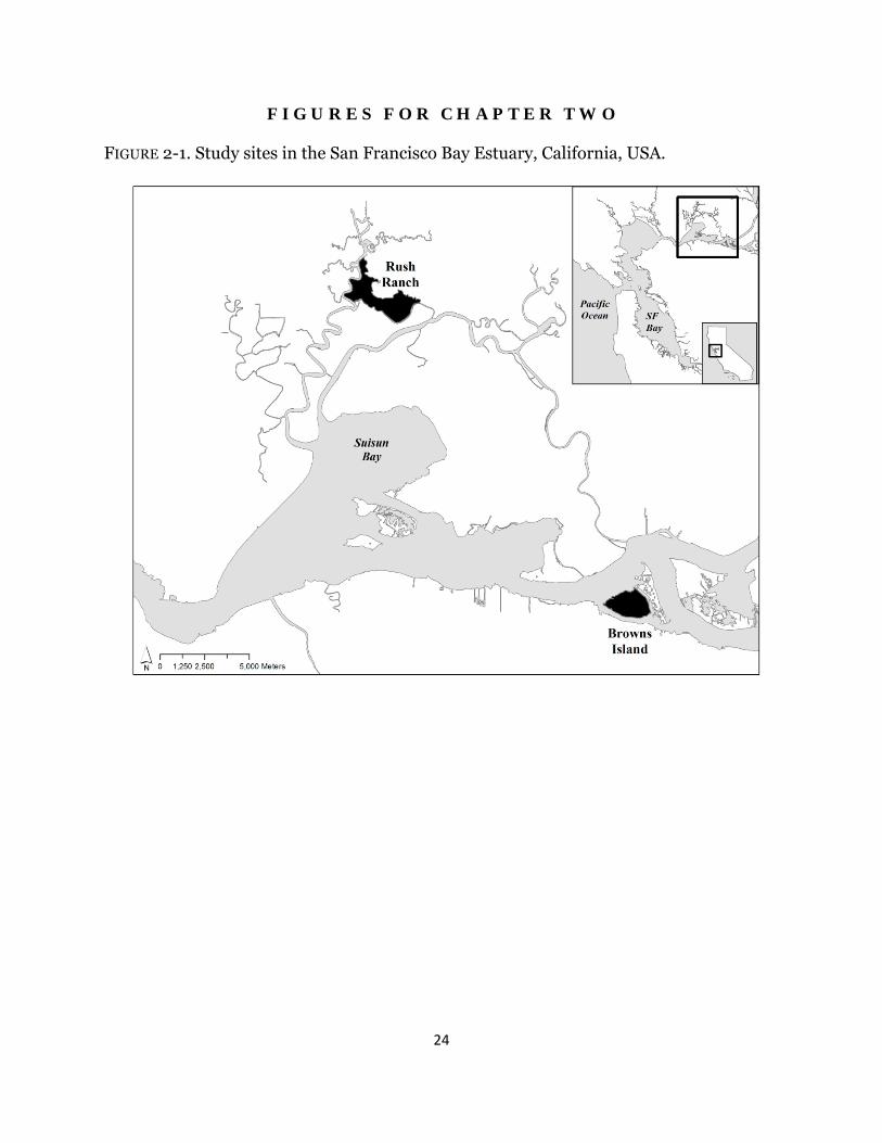
Materials and Methods Site Description I conducted the experiment within two historic brackish tidal wetlands: Browns Island (latitude: 38°2′ N, longitude: 121°51′ W) and Rush Ranch Open Space Preserve (here-after called Rush Ranch; latitude: 38°11′ N, longitude: 122°01′ W (Fig. 2-1). Both sites have mixed semi-diurnal tides. Water salinity fluctuates seasonally, with the lowest and highest salinities found in the early spring and early fall, respectively, and the magnitude depends on winter precipitation and river flow (Enright and Culberson 2009). The average water salinity between 2008 and 2011 was 1.5 and 4.3 ‰ at Browns Island and Rush Ranch, respectively (L. Schile, unpublished data). Species description Schoenoplectus acutus (hardstem tule) dominates along tidal channel, river, and lake margins and forms stands of erect 1.5-3 m tall stems. Rhizomes are 1.5-4 cm wide and grow linearly with few branches (Wildová et al. 2007). Schoenoplectus americanus (Olney’s bulrush) forms solid stands across mid and high marshes. Stems are 0.3-1.8 m tall, and rhizomes are 0.5-2 cm wide, forming both clumps and runners (Ikegami et al. 2007). Both species reproduce predominantly through clonal growth. Experimental Design Experimental planters, named marsh organs (Morris 2007), were constructed to grow both species at five fixed elevations in tidal channels (Fig. 2-2). I established three species treatments at each elevation: one rhizome of each species was planted individually and one rhizome of each species was planted together to examine the role of biotic interactions. To construct marsh organs, 15 cm diameter PVC pipes were cut into five different lengths in 15 cm increments from 45 to 105 cm, window screens were glued to each pipe bottom to allow for drainage, and pipes were bolted together in rows of three in descending height to form a flat-bottomed structure and bolted into a wood frame. At each wetland, seven south-facing channel locations were chosen adjacent to the marsh edge, and three support beams were pounded to resistance into the channel bottom, onto which the marsh organ was mounted. The top row elevation was set at 1.5 m NAVD88, which was determined based on the lower range of marsh elevations for S. acutus and S. americanus, and surveyed using a real-time kinetic global positioning system unit with vertical accuracy of 2-5 cm. Sediment to fill the pipes was collected from unvegetated mudflats within each marsh. Rhizome and Data Collection In April 2010, rhizomes of both species were collected from multiple locations at Browns Island, washed, and grown in fresh water in a greenhouse. In February 2011, all rhizomes and shoots were clipped to a standard length and weighed, and rhizomes were planted at both sites in early March. Every month from April to September 2011, each stem was measured and total stem length and stem density was calculated. Pore-water salinity, pore-water sulfides, and redox potential were collected at both sites within the same week. In one randomly-selected pipe in every row, pore-water was collected 15 cm deep. Salinity was measured and two to five mL of pore-water was mixed immediately with a sulfur anti-oxidant buffer solution in a vacuum-evacuated vial. Sulfide

 

19  

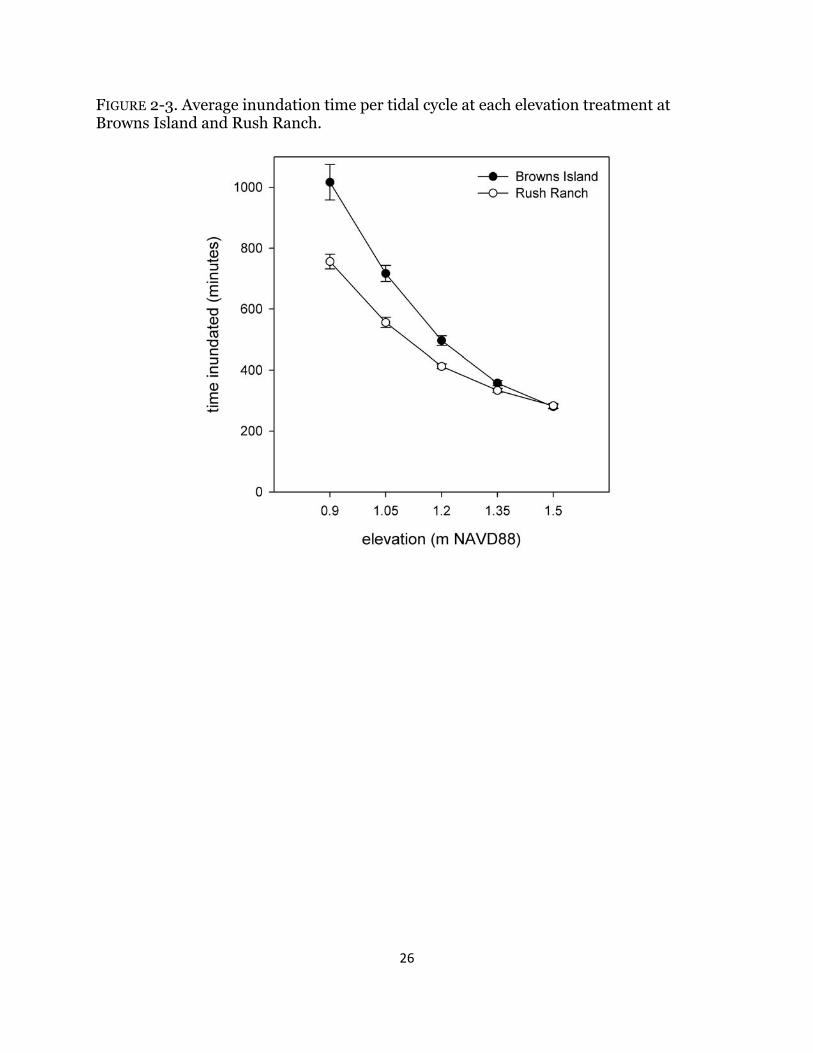
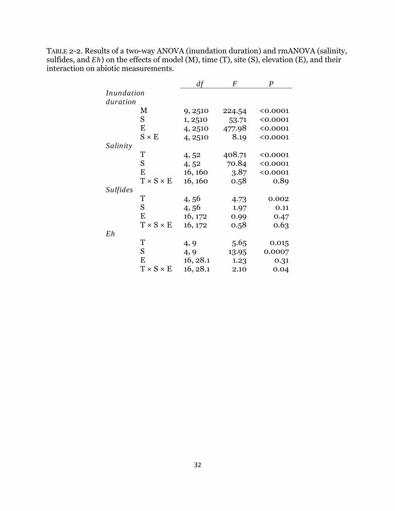
concentrations were measured in the lab and compared against a standard curve. One organ at each site was randomly chosen to collect redox measurements, Eh, in every pipe. Platinum-tipped redox electrodes were placed 15 cm deep, left for a day to equilibrate, and measurements were taken during the bottom of the low tide. Eh was calculated by adding the field voltage to a correction factor for the reference electrode (+200 mV). No pore-water or Eh measurements were taken in August. Channel water level stations were installed at both sites and recorded water salinity and depth every 15 minutes relative to meters NAVD88. The time inundated was calculated for each marsh organ elevation at both sites between March and September and common tidal metrics were computed. Beginning at the end of September through the beginning of November, all above-ground biomass was clipped, and marsh organ pipes were removed. Above-ground biomass was washed, sorted by species and live and dead shoots, dried at 70°C for two days, and weighed. Below-ground biomass was removed from the pipes, washed thoroughly over a 2-mm screen, sorted by species, roots, and rhizomes, dried at 70°C for three days, and weighed. Data Analysis All data were analyzed using SAS 9.2 (SAS 2009); data transformations, when needed, are noted below, and all data met conditions of normality and homogeneity of variance. All post-hoc comparisons were made using Tukey’s least square means test. To examine differences in abiotic variables, the average number of minutes that each elevation treatment was inundated was analyzed using a two way analysis of variance (ANOVA). The data were log transformed. The effects of elevation and site on pore-water salinity, sulfides, and Eh over time were analyzed using a repeated-measures ANOVA (rmANOVA). Salinity and sulfides were square-root transformed. A simple linear regression was run to test for effects of initial wet biomass on total harvested plant biomass. To address my first hypothesis at each site, differences in above-ground, below-ground, total biomass between species and amongst elevations were analyzed using a two-way ANOVA, and all variables were square-root transformed. We ran the same analysis with the same transformation to assess differences in the above-ground, below-ground, and total biomass of plants grown together. To address my second and third hypotheses, the natural log response ratio (lnRR) was calculated at every elevation for each species: lnRR = ln (biomass with neighbors / biomass without neighbors) (Suding et al. 2003). Values less than zero indicate competition, whereas values greater than zero indicate facilitation. The lnRR was calculated for total biomass (above- and below-ground biomass) of each species within every organ row, and the treatment effects of elevation and site were analyzed using a one-way t-test (null expectation zero). Differences in lnRR among species at each elevation and site were analyzed using an ANOVA with planned comparisons. Results Variability in abiotic effects Inundation duration increased significantly with decreasing elevation, and the effect differed by site (Fig. 2-3). The bottom three elevations at Browns Island were inundated

 

20  

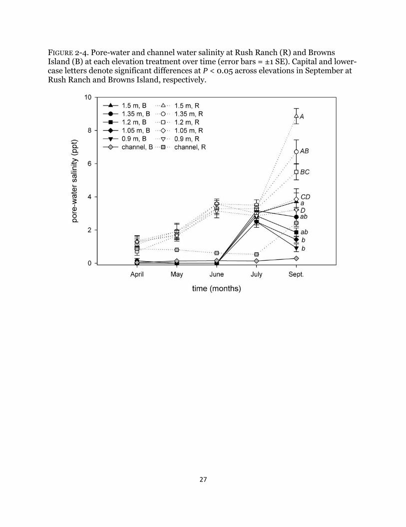
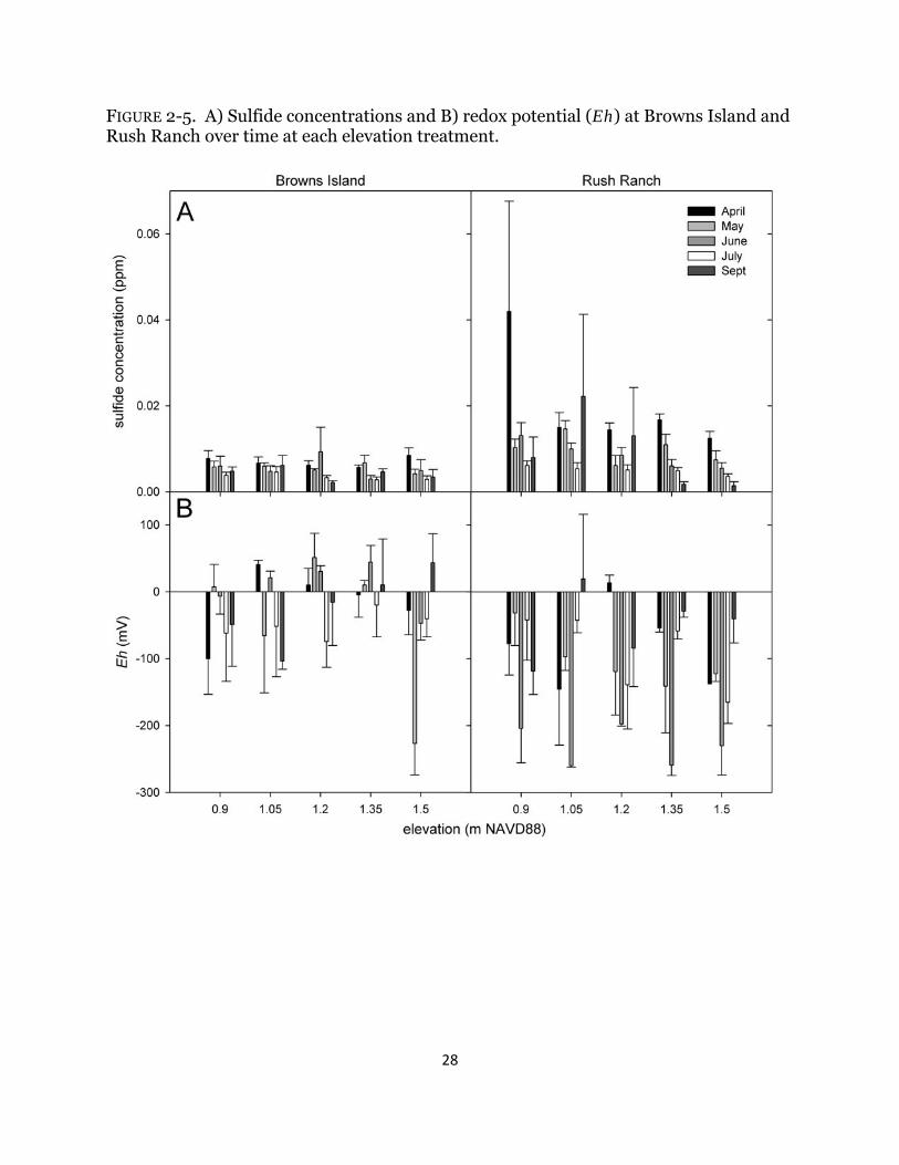
longer than at Rush Ranch (P < 0.004 for all comparisons), although no significant difference was detected between sites at the top two elevations (P > 0.90 for both comparisons). All tidal metrics calculated were greater at Rush Ranch than at Browns Island (Table 2-1), resulting in an increased depth of 11 cm across all elevations. Pore-water salinity was consistently higher at Rush Ranch and increased over time and only varied significantly among elevations in September (Table 2-2; Fig. 2-4). Both pore-water sulfide concentrations and Eh varied over time but there was no consistent or significant trend (Table 2-2; Fig. 2-5). Combined, sulfide concentrations were higher at Rush Ranch than Browns Island, but only marginally (P = 0.0663). Abiotic effects on biomass There was no significant relationship between the initial biomass and total harvested biomass for S. americanus (data not shown; Browns Island: F1,68 = 1.25, P = 0.27; Rush Ranch: F1,68 = 0.33, P = 0.57) or for S. acutus at Browns Island (F1,68 = 1.69, P = 0.20). There was a significant relationship for S. acutus at Rush Ranch; however, initial biomass explained very little variation in the final total biomass (F1,67 = 4.56, P = 0.036; R2 = 0.05).

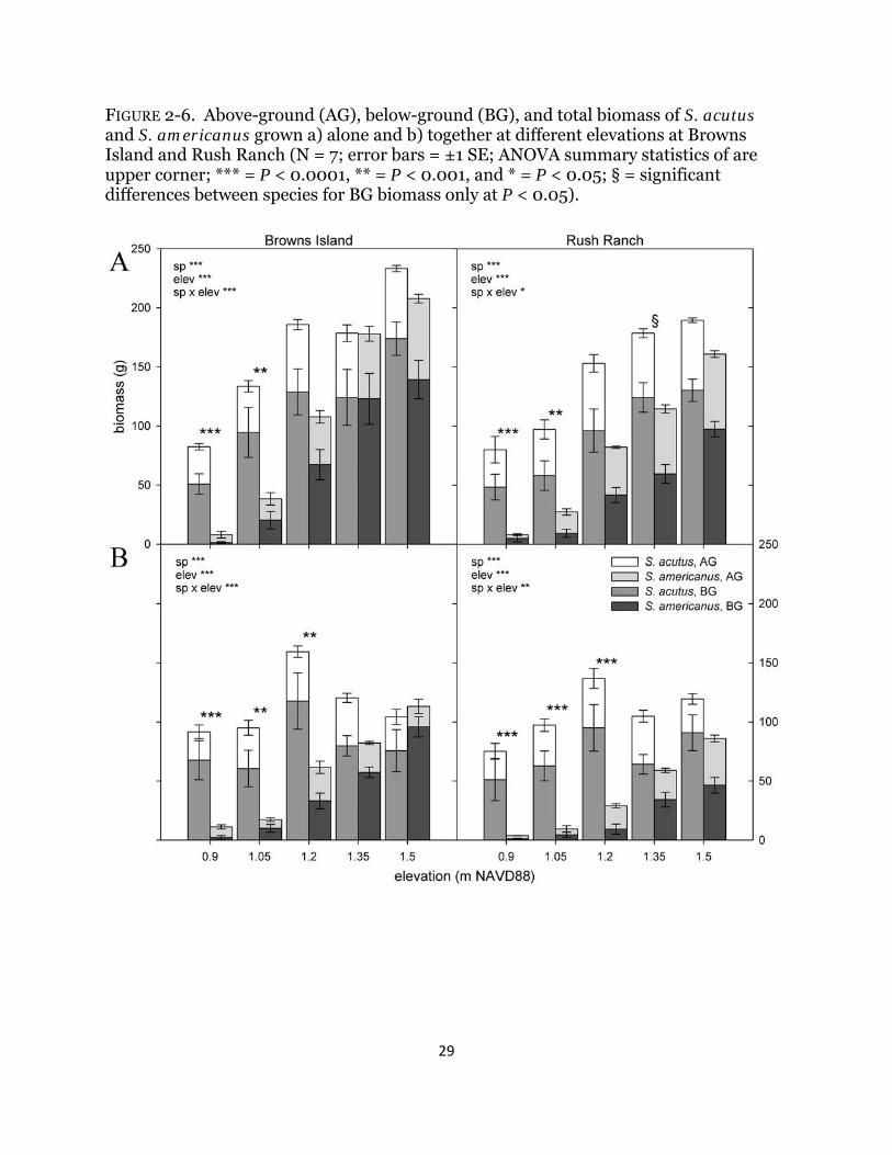
When grown alone, S. americanus had a greater reduction in biomass with increased inundation at both sites than S. acutus (Browns Island: F9,70 = 7.37, P < 0.0001; Rush Ranch: F9,69 = 3.00, P = 0.03; Fig. 2-6a). Total biomass of S. acutus was markedly greater than its congener at the bottom two elevations at both sites (Fig. 2-6a). Total biomass of S. americanus at both sites decreased significantly with decreasing elevation (P < 0.03) except that the top two and subsequent lower pair did not differ significantly (P > 0.2). At Browns Island, total biomass of S. acutus at the lowest elevation was significantly less than its biomass at all other elevations (P < 0.03) except for the elevation above it (P = 0.7); otherwise, total biomass did not differ significantly across elevations (P > 0.7). At Rush Ranch, S. acutus biomass did not differ across the top three or bottom three elevations (P > 0.4) but biomass was greater in the top two elevations than the bottom two (P < 0.02). Similar trends were detected with above- and below-ground biomass (Table 2-3).

When grown together, S. americanus similarly had a greater reduction in biomass than S. acutus with increased inundation at both sites (Browns Island: F9,67 = 8.53, P < 0.0001; Rush Ranch: F9,69 = 3.96, P = 0.006; Fig. 2-6b). Total biomass of S. americanus was significantly lower than S. acutus at the lowest three elevations within each site (P < 0.001; Fig. 2-6b). At both sites, total biomass of S. americanus significantly declined with decreasing elevation in that biomass at each elevation was greater than those below (P < 0.02) but not different than the elevation directly above it (P > 0.2). Total biomass of S. acutus did not differ significantly across elevations within either site (P > 0.2). Similar trends were observed with above- and below-ground biomass (Table 2-3).

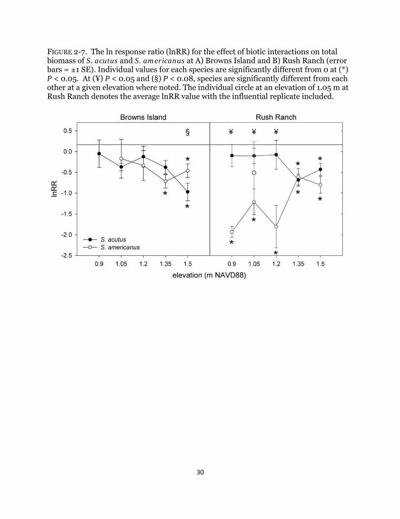
Biotic effects on biomass The presence of neighbors reduced total biomass of both species, particularly at the highest elevation, and biomass did not increase with the presence of neighbors at any elevation across both sites (Table 2-4; Figs. 2-6b & 2-7). Schoenoplectus acutus was more negatively affected by the presence of its congener at the highest elevation at

 

21  

Browns Island compared to any other site/elevation combination (Table 2-4; Fig. 2-7). Although the lnRR for S. acutus was significantly lower than zero (indicating a reduction of biomass and competitive effects) over the top two elevations at Rush Ranch, it did not perform worse than S. americanus at any elevation (Table 2-4; Fig. 2-7). At Rush Ranch, the saltier site, the lnRR for S. americanus was significantly lower than zero for all but one elevation, and S. americanus was more negatively affected by competition compared to its congener at the lowest three elevations (Table 2-4; Fig. 2-7); biomass at the fresher site, Browns Island, was reduced only at the top two elevations. The average lnRR for S. americanus at the middle elevation at Rush Ranch was influenced strongly by one replicate where plant performance was exceptionally great in the presence of S. acutus compared to that when grown alone (Fig. 2-7). The replicate was not found to be an outlier (Grubb’s test for outliers, G = 1.68 standard deviations from the mean), but when it was removed from the analysis, a significant negative effect of competition was detected (t2 = -4.97, P = 0.04) and the species performed worse than its congener (F1,7 = 8.34; P = 0.02; Fig. 2-7). Discussion Influence of increased inundation on biomass My first objective was to document individual plant responses to increased inundation under field conditions and I detected different effects on the biomass of both species. The trend was consistent across wetlands with different salinity regimes, although the magnitude was greater at the saltier site. In support of my first hypothesis, S. acutus, the low marsh species, was better adapted to increased inundation both with and without neighbors and could tolerate growing at elevations 80 cm lower than its current average marsh elevation. Biomass of the marsh plain species S. americanus, however, was greatly reduced when grown with increased inundation and decreased even more when grown with S. acutus; surviving plants had a 93% reduction in biomass (Fig. 2-6). These findings are comparable to other studies that investigated the response S. americanus to abiotic stress (Seliskar 1990, Broome et al. 1995, Kirwan and Guntenspergen 2012). Despite a reduction in biomass at the lowest elevations, both species still displayed a remarkably broad tolerance to increased average inundation up to eight hours in duration (Fig. 2-3). Importance of biotic interactions along stress gradients I predicted that S. americanus would have greater biomass and competitive ability at higher elevations due to its rhizome morphology and overall marsh dominance (hypothesis 2), yet my data reflect this only with the most benign conditions in this experiment: the top elevation at the fresher site (Figs. 2-6 & 2-7). Within the marsh organs, S. americanus was grown at elevations that were lower than its current marsh distribution; therefore, any consistent competitive advantage could have been overwhelmed by negative inundation effects and salinity. At the two lowest organ elevations at Browns Island, S. americanus had a reduction in biomass and this appeared to be due to inundation stress and not competitive interactions (Fig. 2-7). Greiner La Peyre et al. (2001) documented a similar pattern with fresh and brackish marsh plants with increased salinity stress. At the saltier site, however, S. americanus was competitively inferior to the stress tolerator, S. acutus, across most elevations (Fig.

 

22  

2-7), and the negative effect of competition was amplified with increased inundation. This result is contrary to what I predicted (hypothesis 3) and an unexpected result: facilitation, which has been shown to increase with increased abiotic stress in salt, brackish, and freshwater marshes in other regions (Bertness and Callaway 1994, Halpern et al. 2007, Luo et al. 2010, Guo and Pennings 2012), was not detected at any elevation. Soil redox potential did not differ significantly across elevations (Fig. 2-5) suggesting no detectible change in root soil aeration, which could have ameliorated stress from soil anaerobicity (Hacker and Bertness 1999). Implications with climate change This experiment increased inundation depths between 0.2 and 0.9 m relative to current average plant elevations, values that are within the lower range of 2100 predictions of 0.4 to 1.8 m increases (Vermeer and Rahmstorf 2009), and I documented significant negative effects on plant biomass and community interactions. Wetlands will respond to increases in sea level through increased sediment deposition (Morris et al. 2002) and plant growth (Cherry et al. 2009, Langley et al. 2009) to maintain their elevation. These factors, combined with upland migration, would reduce the negative impact of increasing sea levels. However, there are limits to these responses (Kirwan et al. 2010), and growing evidence suggests that a reduction in suspended sediment concentrations (Ibàñez et al. 1996, Cloern et al. 2011), reduced biomass due to individual plant responses and competitive interactions (this study), and a limited amount of available upland habitat (Stralberg et al. 2011) present a future of shifting plant dominance, restriction in distribution, and reduction in wetland extent. I documented a decrease in biomass in both species at the site with higher channel water and pore-water salinities (Table 2-2; Fig. 2-4), and the difference in channel water salinity was only 3 ‰. I likely can attribute the reduced biomass to increased salinity since other environmental factors did not differ significantly between sites (Table 2-2), although I cannot say this conclusively due to the absence of replicate sites within each salinity range in this estuary. Water salinity in the San Francisco Bay estuary, as with other estuaries, is variable among years and with freshwater management practices and concentrations are predicted to increase between 3 and 5 ‰ by 2100 (Cloern et al. 2011). Estuary-level decreases in biomass are likely to occur as a result of combined increases in inundation and salinity, and previous work has documented decreases in site-level biomass with increased salinity (Crain et al. 2004, Craft et al. 2008). The implications for marsh sustainability and carbon sequestration under increased inundation depths are significant. I observed a reduction in biomass for both species examined, which implies a reduced carbon stock for below-ground sequestration and a decrease in the organic matter contribution to marsh accretion. When species are exposed to the stressor that is ultimate limiting at the edge of its range, differential effects of biotic interactions might occur (Maestre et al. 2009, Guo and Pennings 2012). I did not demonstrate shifts in the nature of biotic interactions in this study and found that increased inundation, competition, and salinity compromised the ability of both species, particularly the mid marsh species, to grow. My results point to the importance of synergies between multiple stressors, which are predicted to increase in intensity with

 

23  

climate change, that can differentially influence the relative abiotic and competitive forces on biomass as stresses increase.

 

24  

F I G U R E S F O R C H A P T E R T W O

FIGURE 2-1. Study sites in the San Francisco Bay Estuary, California, USA.

 

25  

FIGURE 2-2. Example of an installed marsh organ before sediment and plants were added.

 

26  

FIGURE 2-3. Average inundation time per tidal cycle at each elevation treatment at Browns Island and Rush Ranch.

 

27  

FIGURE 2-4. Pore-water and channel water salinity at Rush Ranch (R) and Browns Island (B) at each elevation treatment over time (error bars = ±1 SE). Capital and lower-case letters denote significant differences at P < 0.05 across elevations in September at Rush Ranch and Browns Island, respectively.

 

28  

FIGURE 2-5. A) Sulfide concentrations and B) redox potential (Eh) at Browns Island and Rush Ranch over time at each elevation treatment.

 

29  

FIGURE 2-6. Above-ground (AG), below-ground (BG), and total biomass of S. acutus and S. americanus grown a) alone and b) together at different elevations at Browns Island and Rush Ranch (N = 7; error bars = ±1 SE; ANOVA summary statistics of are upper corner; *** = P < 0.0001, ** = P < 0.001, and * = P < 0.05; § = significant differences between species for BG biomass only at P < 0.05).

 

30  

FIGURE 2-7. The ln response ratio (lnRR) for the effect of biotic interactions on total biomass of S. acutus and S. americanus at A) Browns Island and B) Rush Ranch (error bars = ±1 SE). Individual values for each species are significantly different from 0 at (*) P < 0.05. At (¥) P < 0.05 and (§) P < 0.08, species are significantly different from each other at a given elevation where noted. The individual circle at an elevation of 1.05 m at Rush Ranch denotes the average lnRR value with the influential replicate included.

 

31  

T A B L E S F O R C H A P T E R T W O TABLE 2-1. Tidal metrics in meters NAVD88 at the study sites (MHHW = mean higher high water; MHW = mean high water; MLHW = mean lower high water; MTL = mean tide level; MHLW = mean higher low water; MLW = mean low water; MLLW = mean lower low water).

Site MHHW MHW MLHW MTL MHLW MLW MLLW Browns Island 1.90 1.76 1.62 1.31 1.03 0.84 0.63 Rush Ranch 2.01 1.87 1.73 1.29 0.93 0.69 0.46

 

32  

TABLE 2-2. Results of a two-way ANOVA (inundation duration) and rmANOVA (salinity, sulfides, and Eh) on the effects of model (M), time (T), site (S), elevation (E), and their interaction on abiotic measurements.

df F P Inundation duration

M 9, 2510 224.54 <0.0001 S 1, 2510 53.71 <0.0001 E 4, 2510 477.98 <0.0001 S × E 4, 2510 8.19 <0.0001

Salinity T 4, 52 408.71 <0.0001 S 4, 52 70.84 <0.0001 E 16, 160 3.87 <0.0001 T × S × E 16, 160 0.58 0.89

Sulfides T 4, 56 4.73 0.002 S 4, 56 1.97 0.11 E 16, 172 0.99 0.47 T × S × E 16, 172 0.58 0.63

Eh T 4, 9 5.65 0.015 S 4, 9 13.95 0.0007 E 16, 28.1 1.23 0.31 T × S × E 16, 28.1 2.10 0.04

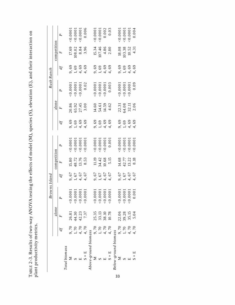
       33TA

BL

E 2

-3. R

esu

lts

of t

wo-

way

AN

OV

A t

esti

ng

the

effe

cts

of m

odel

(M

), s

pec

ies

(S),

ele

vati

on (

E),

an

d t

hei

r in

tera

ctio

n o

n

pla

nt

pro

du

ctiv

ity

met

rics

.

Bro

wn

s Is

lan

d

R

ush

Ra

nch

al

one

com

pet

itio

n

alon

e co

mp

etit

ion

d

f F

P

d

f F

P

d

f F

P

d

f F

P

T

ota

l bio

ma

ss

M

9, 7

0

26.8

1 <

0.0

00

1 9

, 67

15.8

0

<0

.00

01

9, 6

9 20

.86

<0

.00

01

9, 6

9

17.6

9 <

0.0

00

1 S

1, 7

0

44.3

0

<0

.00

01

1, 6

7 4

8.7

2 <

0.0

00

1 1,

69

6

5.9

2 <

0.0

00

1 1,

69

108

.02

<0

.00

01

E

4, 7

0

42.2

3 <

0.0

00

1 4,

67

13.7

6 <

0.0

00

1 4,

69

27

.45

<0

.00

01

4, 6

9 8

.84

<0

.00

01

S ×

E

4, 7

0

7.37

<

0.0

00

1 4,

67

8.5

3 <

0.0

00

1 4,

69

3.

00

0

.02

4, 6

9

3.9

6 0

.00

6

Abo

ve-g

rou

nd

bio

ma

ss

M

9, 7

0

25.3

5 <

0.0

00

1 9

, 67

11.1

9

<0

.00

01

9, 6

9 14

.60

<

0.0

00

1 9

, 69

15

.34

<0

.00

01

S 1,

70

33

.13

<0

.00

01

1, 6

7 34

.42

<0

.00

01

1, 6

9

54.6

1 <

0.0

00

1 1,

69

10

7.46

<

0.0

00

1 E

4,

70

38

.10

<

0.0

00

1 4,

67

10.6

8

<0

.00

01

4, 6

9

14.5

9 <

0.0

00

1 4

, 69

4

.86

0.0

02

S ×

E

4, 7

0

10.7

8

<0

.00

01

4, 6

7 5.

15

0.0

01

4, 6

9

4.6

2 0

.00

3 4

, 69

2.

80

0

.03

Bel

ow-g

rou

nd

bio

ma

ss

M

9, 7

0

22.0

6

<0

.00

01

9, 6

7 14

.68

<

0.0

00

1 9

, 69

22

.31

<0

.00

01

9, 6

9

18.0

8

<0

.00

01

S 1,

70

39

.28

<

0.0

00

1 1,

67

42.

77

<0

.00

01

1, 6

9 6

4.0

8

<0

.00

01

1, 6

9

103.

38

<0

.00

01

E

4, 7

0

35.1

5 <

0.0

00

1 4,

67

13.2

2 <

0.0

00

1 4,

69

32

.11

<0

.00

01

4, 6

9

10.5

2 <

0.0

00

1 S

× E

4,

70

5.

04

0.0

01

4, 6

7 8

.18

<

0.0

00

1 4,

69

2.

06

0

.09

4,

69

4.

31

0.0

04

 

       34TA

BL

E 2

-4. R

esu

lts

of t

he

lnR

R t

est

for

the

dir

ecti

on a

nd

str

engt

h o

f bi

otic

inte

ract

ion

s an

d s

pec

ies

dif

fere

nce

s on

tot

al

pla

nt

biom

ass

wh

en g

row

n a

t B

row

ns

Isla

nd

(B

) an

d R

ush

Ran

ch (

R)

acro

ss f

ive

elev

atio

ns.

(*

see

resu

lts

abou

t re

mov

al o

f ou

tlie

r)

S. a

cutu

s

S. a

mer

ica

nu

s

Spec

ies

com

par

ison

Site

el

evat

ion

(m

) d

f t-

valu

e P

d

f t-

valu

e P

d

f F

P

B

0

.90

6

0

.62

0.5

6 1

- -

1, 6

1.

32

0.2

9 B

1.

05

6

-2.3

4

0.0

5 4

-0.3

7 0

.73

1, 1

0

0.8

0

.39

B

1.

20

6

-0.4

9

0.6

4 5

-0.9

3 0

.39

1,

11

0.2

5 0

.63

B

1.35

6

-2

.34

0

.05

6

-4.4

0

.00

5 1,

12

2.2

0.1

6 B

1.

50

5 -4

.58

0

.00

6 5

-2.8

2 0

.04

1, 1

0

2.7

0.0

8

R

0.9

0

6

-0.3

7 0

.72

1 -1

4.9

3 0

.04

1, 7

12

.18

0

.01

R

1.0

5 5

-0.5

6 0

.60

3*

-0

.68

0

.55

1, 8

* 0

.4

0.5

4 R

1.

20

6

-0.2

2 0

.83

5 -3

.52

0.0

2 1,

11

8.1

2 0

.02

R

1.35

6

-4

.76

0

.00

3 6

-3

.06

0

.02

1, 1

2 0

.11

0.7

5 R

1.

50

6

-2.9

2 0

.03

6

-4

0.0

07

1, 1

2 2.

23

0.1

6  

 

35  

C H A P T E R T H R E E

Accounting for non-photosynthetic vegetation in remote sensing based estimates of carbon flux in wetlands

Monitoring productivity in coastal wetlands is important due to their high carbon sequestration rates and potential role in climate change mitigation. I tested agricultural- and forest-based methods for estimating the fraction of absorbed photosynthetically active radiation (ƒAPAR), a key parameter for modeling gross primary productivity (GPP), in a restored managed wetland with a dense litter layer of non-photosynthetic vegetation, and I compared the difference in canopy light transmission between a tidally influenced wetland and the managed wetland. The presence of litter reduced correlations between spectral vegetation indices and ƒAPAR. In the managed wetland, a two-band vegetation index incorporating simulated World View-2 or Hyperion green and near infrared bands collected with a field spectroradiometer significantly correlated with fAPAR only when measured above the litter layer and not at the ground where measurements typically occur. Measures of GPP in these systems are difficult to capture via remote sensing, and require an investment of sampling effort, practical methods for measuring green leaf area, and accounting for background effects of litter and water. Introduction Understanding carbon dynamics in ecosystems, specifically plant production and carbon sequestration, is of increasing significance in light of accelerated climate change (Crooks et al. 2010). In particular, monitoring carbon in freshwater wetlands (temperate peatlands) is critical, as they generate among the greatest annual rates of net primary productivity and soil carbon storage in natural ecosystems (Miller and Fujii 2010). With the added importance of mitigating climate change and offsetting greenhouse gas emissions, policy makers are focusing on these wetlands and opportunities for their restoration, preservation, and avoiding their loss (Crooks et al. 2010), since they often have been modified, degraded, and/or destroyed (Deverel and Rojstaczer 1996, Tornqvist et al. 2008). Managed restoration of subsided peatlands is considered one of the more promising climate change mitigation activities for wetland ecosystems (Emmett-Mattox et al. 2011). Remote sensing, which has been used often for long-term monitoring of changes in wetland area (Byrd et al. 2004, Tuxen et al. 2007), vegetation classification (Klemas 2011) and carbon stocks (Ravindranath and Ostwald 2007), might help in addressing the need to estimate the productivity of these restored wetlands. Extensive field measurements of plant biophysical characteristics such as live biomass, leaf area index (LAI), and fraction of absorbed photosynthetically active radiation (ƒAPAR) have been collected in agricultural systems (Gitelson 2012, Peng and Gitelson 2012) and forests (Maselli et al. 2009, Penuelas et al. 2011, Wu et al. 2012). Whereas such vegetation metrics can be measured in wetlands, linking these field measurements

 

36  

to remotely sensed data and generating estimates at regional scales are challenging due to the small size, local spatial variability, and varying seasonal and annual patterns of wetlands and wetland vegetation (Phinn 1998, Zhang et al. 1997). In addition, background effects of senesced non-photosynthetic vegetation (litter), floating aquatic vegetation, and inundation influence the relationship between spectral reflectance and field measurements (Kearney et al. 2009, Numata 2012). Litter and soil have high spectral signatures throughout the 400-2500 nanometer (nm) range and can dominate the reflectance of canopies of low coverage; therefore, neglecting these background effects can generate erroneous estimation of biophysical characteristics such as biomass when using remotely sensed data (Numata 2012). Integrating the effect of all physiologically active absorbing pigments present in a vegetated canopy, ƒAPAR is a key variable in light use efficiency (LUE) and other plant productivity models (Middleton et al. 2012) that relates canopy structure to function from the leaf to landscape scale (Asner et al. 1998). Accurate ƒAPAR measurements are important to the performance of LUE models and estimates of gross primary productivity (GPP) (Cook et al. 2009, Middleton et al. 2012) and need to be adjusted for the proportion of green leaf area to total leaf area, which is complicated when there is a significant amount of litter (Gitelson 2012, Middleton et al. 2012). ƒAPAR can be estimated from spectral indices such as the normalized difference vegetation index (NDVI) or simple band ratios but it is affected by background effects (Todd and Hoffer 1998). Different NDVI-type two band vegetation indices (TBVIs) using band combinations other than red and near infra-red (NIR) may perform better. A TBVI for bands i and j is calculated according to equation (1):

TBVIij = (Rj - Ri) ⁄ (Rj + Ri) where Ri and Rj are the reflectance values of bands i and j

Findings within irrigated rice fields (Inoue et al. 2008) suggest highly linear relationships with ƒAPAR using blue (410 and 420 nm) or green (550 nm) and near-infrared (720 nm) wavelengths for an entire growing period, with no dependence on phenology; however, rice fields have no standing litter and very distinct growth and senescence periods, where the effect of litter is separated in time as opposed to natural ecosystems. The goal of this study was to test the application of agricultural- and forest-based methods for estimating ƒAPAR in a heterogeneous wetland environment with a significant litter layer. My main questions were: 1) How does the presence of dense litter influence light transmission through the canopy? 2) How does ƒAPAR in a managed restored wetland compare to a tidally influenced wetland with a sparse litter layer? 3) How does the presence of a dense litter layer influence the strength of correlation between ƒAPAR and hyperspectral and multispectral indices calculated with field spectrometer reflectance data? Answers to these questions will inform wetland managers of the accuracies and errors associated with the use of remote sensing for wetland productivity estimates.

 

37  

Methods Site Description Field measurements were collected at two sites in the Sacramento-San Joaquin River Delta, San Francisco Bay Estuary, California, USA: Twitchell Island and Sherman Lake (Fig. 3-1). Sampling at Twitchell Island (38º 6’ N, 121º 39’ W) was completed within a 6-ha experimental freshwater wetland system created in 1997 to examine hydrologic controls on peat accretion and carbon sequestration rates (Miller et al. 2008, Miller and Fujii 2010). A network of boardwalks was built within the wetland to reduce disturbance. Twitchell Island is dominated by Schoenoplectus acutus and a variety of Typha species and their hybrids. Schoenoplectus acutus is characterized by tall rounded green stems growing one to four meters tall with an erectophile leaf angle distribution that maximizes exposure to light and photosynthetic rates (Rocha and Goulden 2009). Because the site is managed for maximizing peat accretion, a dense litter layer one to two meters tall, composed primarily of dead S. acutus stems, has accumulated over several years. In contrast, Sherman Lake (38º 02’ N, 121º 48’ W) is a freshwater tidal wetland with a similar species composition along channel edges. The site was chosen to test if litter densities were different in a tidally influenced site and how litter influences light transmission through the canopy and associated ƒAPAR measurements. Data Collection Ground-based measurements Twenty nine 1 m2 field plots were established across Twitchell Island within 1.5 m of a boardwalk; 15 plots were established along tidal channel edges at Sherman Lake. Data collection for ƒAPAR calculations occurred at Twitchell Island on 22 July and 30 September 2011 and at Sherman Lake on 23 October 2011. Measurements were collected during a high tide at Sherman Lake to replicate water conditions at Twitchell Island. A LI-COR LI-190 point quantum sensor and a LI-COR LI-191 line quantum sensor were used to collect PARincoming (Qb) and PARtransmitted (Qa), respectively, where PAR is photosynthetically active radiation. At Twitchell Island, live stem height and diameter were measured to calculate LAI and biomass using allometric equations (Miller and Fujii 2010). Water depth was measured in all plots and ranged from 10 to 110 cm. Within each plot, three canopy heights were established for measuring Qa: at the top of the litter layer (high), at the water surface (low), and at a mid-litter height halfway between the first two heights (mid; Fig. 3-2). Starting at the water level and moving up, the line quantum sensor was placed at each height and readings were averaged over a 15 second period. Qb was collected immediately after the last Qa measurement. The percentage of live plant material relative to all plant material above and along the sensor length at each elevation was visually estimated in order to calculate ƒAPAR for photosynthetic material (Daubenmire 1959). Given the three Qa measurements, ƒAPAR-high, ƒAPAR-mid, and ƒAPAR-low were calculated and adjusted for the percent coverage of green vegetation (Vl) at each height according to equation (2) (Wharton et al. 2009).

 

38  

ƒAPAR = [1 – (Qa / Qb)]*Vl

Field spectroradiometer readings Together with ƒAPAR measurements, canopy reflectance spectra were obtained at Twitchell Island over each plot near midday using an ASD Inc. FieldSpec Pro FR portable spectroradiometer. Spectral readings were obtained at every 1.4 nm over 350–1000 nm and 2 nm over 1000–2500 nm using a 25° field of view foreoptics. Readings were taken at nadir 4 m above the vegetation canopy using a 3 m optical fiber cable. Spectral reflectance values were derived as the ratio of reflected radiance to incident radiance estimated from the reflected radiance from a calibrated white reference, which was collected every 10 minutes. At each sample location, ten reflectance measurements, each an average of 12 spectra, were collected and then averaged using ViewSpec™ Pro 6.1.10 (Analytical Spectral Devices, Inc, Boulder, CO, USA). Field spectroradiometer data could not be collected at Sherman Lake due to difficult site access. To compare the effectiveness of broadband vs. narrowband indices in predicting ƒAPAR, I simulated eight Digital Globe World View-2 (WV-2) bands and 164 hyperspectral Hyperion bands with the field spectroradiometer data from Twitchell Island. WV-2 bands include a coastal blue, blue, green, yellow, red, red edge, and two near infrared bands and have 2 m spatial resolution. Hyperion is a hyperspectral satellite sensor on the National Aeronautics and Space Administration Earth Observing One (NASA EO-1) with 30 m resolution and 242 bands each 10 nm-wide. The simulated Hyperion bands covered the ranges 422–1300 nm, 1443–1795 nm, and 1998–2400 nm. Water absorption regions of the spectrum with high noise were removed from analysis. For both simulated datasets, I calculated all possible TBVI using all band combinations (Thenkabail et al. 2004) for a total of 28 WV-2 and 13 366 Hyperion indices. Data Analysis Using SAS 9.2 (SAS Inc 2009), I ran a two-way analysis of variance with planned comparisons using arc-sine square-root transformed data to investigate how site, month of measurement at Twitchell, and sensor position within the litter layer influence light transmission through the canopy and ƒAPAR. All post-hoc comparisons were made using Tukey’s least square means test. Using Stata (StataCorp LP 1985-2009), I ran pairwise correlations to calculate the correlation (r) between all TBVIs for both simulated WV-2 and Hyperion bands and the three ƒAPAR values: ƒAPAR-high, ƒAPAR-mid, and ƒAPAR-low. Coefficients of determination (R2) were calculated for the highest TBVI-ƒAPAR

correlations. Linear and second order exponential fits were tested. For band Combinations with the highest correlation at Twitchell Island, I ran multiple linear regressions with water depth and plant biomass as covariates to determine if the strength of the TBVI-ƒAPAR relationship improved.

 

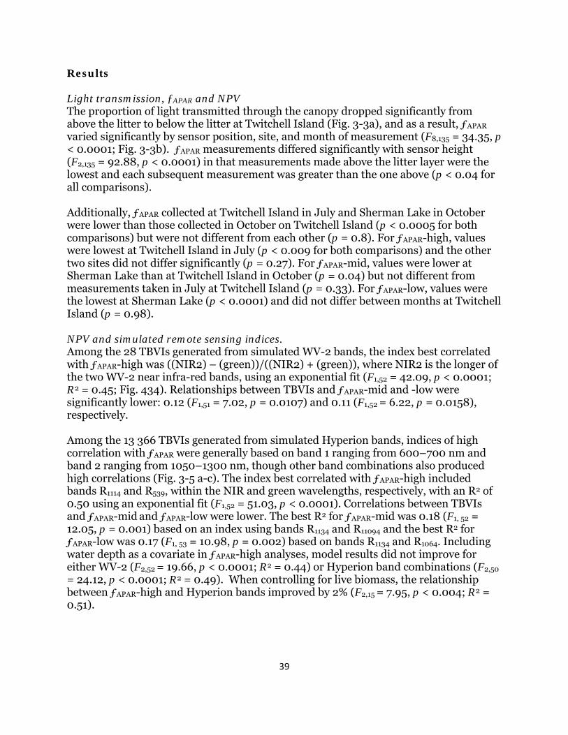
39  

Results Light transmission, ƒAPAR and NPV The proportion of light transmitted through the canopy dropped significantly from above the litter to below the litter at Twitchell Island (Fig. 3-3a), and as a result, ƒAPAR varied significantly by sensor position, site, and month of measurement (F8,135 = 34.35, p < 0.0001; Fig. 3-3b). ƒAPAR measurements differed significantly with sensor height (F2,135 = 92.88, p < 0.0001) in that measurements made above the litter layer were the lowest and each subsequent measurement was greater than the one above (p < 0.04 for all comparisons). Additionally, ƒAPAR collected at Twitchell Island in July and Sherman Lake in October were lower than those collected in October on Twitchell Island (p < 0.0005 for both comparisons) but were not different from each other (p = 0.8). For ƒAPAR-high, values were lowest at Twitchell Island in July (p < 0.009 for both comparisons) and the other two sites did not differ significantly (p = 0.27). For ƒAPAR-mid, values were lower at Sherman Lake than at Twitchell Island in October (p = 0.04) but not different from measurements taken in July at Twitchell Island (p = 0.33). For ƒAPAR-low, values were the lowest at Sherman Lake (p < 0.0001) and did not differ between months at Twitchell Island (p = 0.98). NPV and simulated remote sensing indices. Among the 28 TBVIs generated from simulated WV-2 bands, the index best correlated with ƒAPAR-high was ((NIR2) – (green))/((NIR2) + (green)), where NIR2 is the longer of the two WV-2 near infra-red bands, using an exponential fit (F1,52 = 42.09, p < 0.0001; R2 = 0.45; Fig. 434). Relationships between TBVIs and ƒAPAR-mid and -low were significantly lower: 0.12 (F1,51 = 7.02, p = 0.0107) and 0.11 (F1,52 = 6.22, p = 0.0158), respectively. Among the 13 366 TBVIs generated from simulated Hyperion bands, indices of high correlation with ƒAPAR were generally based on band 1 ranging from 600–700 nm and band 2 ranging from 1050–1300 nm, though other band combinations also produced high correlations (Fig. 3-5 a-c). The index best correlated with ƒAPAR-high included bands R1114 and R539, within the NIR and green wavelengths, respectively, with an R2 of 0.50 using an exponential fit (F1,52 = 51.03, p < 0.0001). Correlations between TBVIs and ƒAPAR-mid and ƒAPAR-low were lower. The best R2 for ƒAPAR-mid was 0.18 (F1, 52 = 12.05, p = 0.001) based on an index using bands R1134 and R11094 and the best R2 for ƒAPAR-low was 0.17 (F1, 53 = 10.98, p = 0.002) based on bands R1134 and R1064. Including water depth as a covariate in ƒAPAR-high analyses, model results did not improve for either WV-2 (F2,52 = 19.66, p < 0.0001; R2 = 0.44) or Hyperion band combinations (F2,50

= 24.12, p < 0.0001; R2 = 0.49). When controlling for live biomass, the relationship between ƒAPAR-high and Hyperion bands improved by 2% (F2,15 = 7.95, p < 0.004; R2 = 0.51).

 

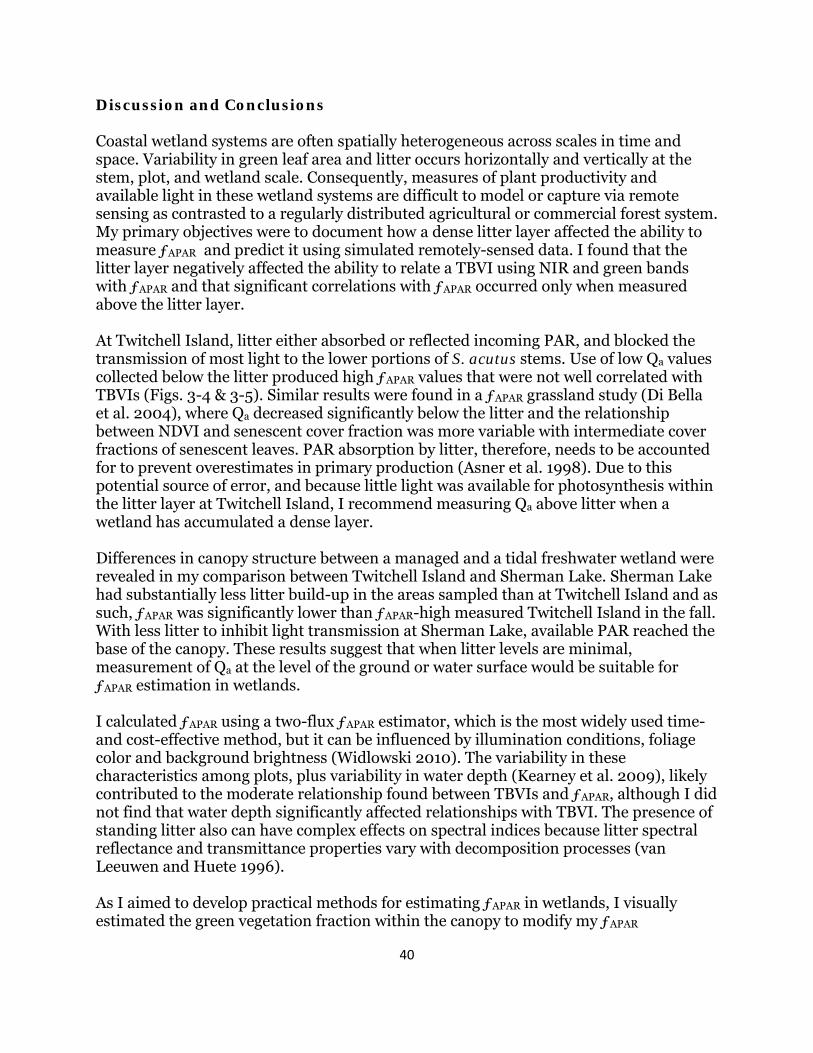
40  

Discussion and Conclusions Coastal wetland systems are often spatially heterogeneous across scales in time and space. Variability in green leaf area and litter occurs horizontally and vertically at the stem, plot, and wetland scale. Consequently, measures of plant productivity and available light in these wetland systems are difficult to model or capture via remote sensing as contrasted to a regularly distributed agricultural or commercial forest system. My primary objectives were to document how a dense litter layer affected the ability to measure ƒAPAR and predict it using simulated remotely-sensed data. I found that the litter layer negatively affected the ability to relate a TBVI using NIR and green bands with ƒAPAR and that significant correlations with ƒAPAR occurred only when measured above the litter layer. At Twitchell Island, litter either absorbed or reflected incoming PAR, and blocked the transmission of most light to the lower portions of S. acutus stems. Use of low Qa values collected below the litter produced high ƒAPAR values that were not well correlated with TBVIs (Figs. 3-4 & 3-5). Similar results were found in a ƒAPAR grassland study (Di Bella et al. 2004), where Qa decreased significantly below the litter and the relationship between NDVI and senescent cover fraction was more variable with intermediate cover fractions of senescent leaves. PAR absorption by litter, therefore, needs to be accounted for to prevent overestimates in primary production (Asner et al. 1998). Due to this potential source of error, and because little light was available for photosynthesis within the litter layer at Twitchell Island, I recommend measuring Qa above litter when a wetland has accumulated a dense layer. Differences in canopy structure between a managed and a tidal freshwater wetland were revealed in my comparison between Twitchell Island and Sherman Lake. Sherman Lake had substantially less litter build-up in the areas sampled than at Twitchell Island and as such, ƒAPAR was significantly lower than ƒAPAR-high measured Twitchell Island in the fall. With less litter to inhibit light transmission at Sherman Lake, available PAR reached the base of the canopy. These results suggest that when litter levels are minimal, measurement of Qa at the level of the ground or water surface would be suitable for ƒAPAR estimation in wetlands. I calculated ƒAPAR using a two-flux ƒAPAR estimator, which is the most widely used time- and cost-effective method, but it can be influenced by illumination conditions, foliage color and background brightness (Widlowski 2010). The variability in these characteristics among plots, plus variability in water depth (Kearney et al. 2009), likely contributed to the moderate relationship found between TBVIs and ƒAPAR, although I did not find that water depth significantly affected relationships with TBVI. The presence of standing litter also can have complex effects on spectral indices because litter spectral reflectance and transmittance properties vary with decomposition processes (van Leeuwen and Huete 1996). As I aimed to develop practical methods for estimating ƒAPAR in wetlands, I visually estimated the green vegetation fraction within the canopy to modify my ƒAPAR

 

41  

calculations, and this potentially was the greatest source of error. For more precise measurements, green leaf and total leaf area should be measured to quantify the fraction of absorbed light that is used for photosynthesis (Gitelson 2012). However, LAI is difficult to quantify accurately due to spatial and temporal variability in leaf qualities (this study, data not shown; Weiss et al. 2004). Direct measurement such as destructive sampling is time consuming while indirect optical methods such as the use of commercial optical instruments have been found to underestimate (Guo and Si 2008) or overestimate (Schile, unpublished data) LAI due to the complexity of natural canopy architecture. My results have implications for successful large-scale accurate quantification of plant productivity in managed restored wetlands. Vegetated indices derived from simulated hyperspectral Hyperion bands performed only slightly better at predicting ƒAPAR than indices derived from simulated broadband WV-2 bands (R2 = 0.50 vs. R2 = 0.45). These results suggest that the WV-2 imagery may be suitable and practical for mapping ƒAPAR, given the challenge of obtaining hyperspectral imagery. In addition, the high spatial resolution of WV-2 (2 m) compared to that of Hyperion (30 m) would enable greater discrimination of green and standing dead vegetation cover in these heterogeneous sites. Coastal vegetated ecosystems including the wetlands described in this study will potentially play a larger role in future climate change mitigation due to their large carbon sequestration potential (Crooks et al. 2010, Pendleton et al. 2012). Accurate landscape scale estimates of ƒAPAR will require a greater investment in sampling effort, practical methods for quantifying green leaf area, and quantifying the effects of litter and water inundation on vegetation indices, which will aid in the development of robust indices that can be applied to other wetland sites and across larger extents for estimates of productivity and carbon storage potential.

 

42  

F I G U R E S F O R C H A P T E R T H R E E FIGURE 3-1. Sherman Lake and Twitchell Island in the Sacramento-San Joaquin River Delta, California, USA.

 

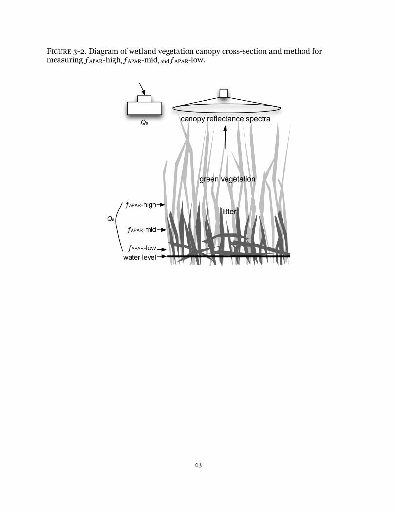
43  

FIGURE 3-2. Diagram of wetland vegetation canopy cross-section and method for measuring ƒAPAR-high, ƒAPAR-mid, and ƒAPAR-low.

 

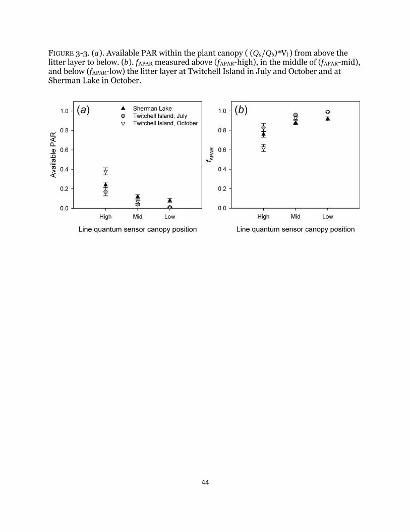
44  

FIGURE 3-3. (a). Available PAR within the plant canopy ( (Qa/Qb)*Vl ) from above the litter layer to below. (b). fAPAR measured above (fAPAR-high), in the middle of (fAPAR-mid), and below (fAPAR-low) the litter layer at Twitchell Island in July and October and at Sherman Lake in October.

 

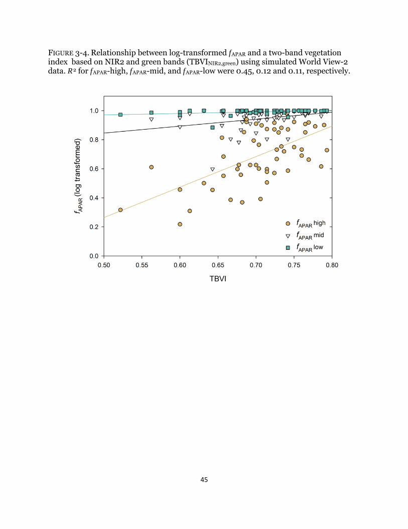
45  

FIGURE 3-4. Relationship between log-transformed fAPAR and a two-band vegetation index based on NIR2 and green bands (TBVINIR2,green) using simulated World View-2 data. R2 for fAPAR-high, fAPAR-mid, and fAPAR-low were 0.45, 0.12 and 0.11, respectively.

 

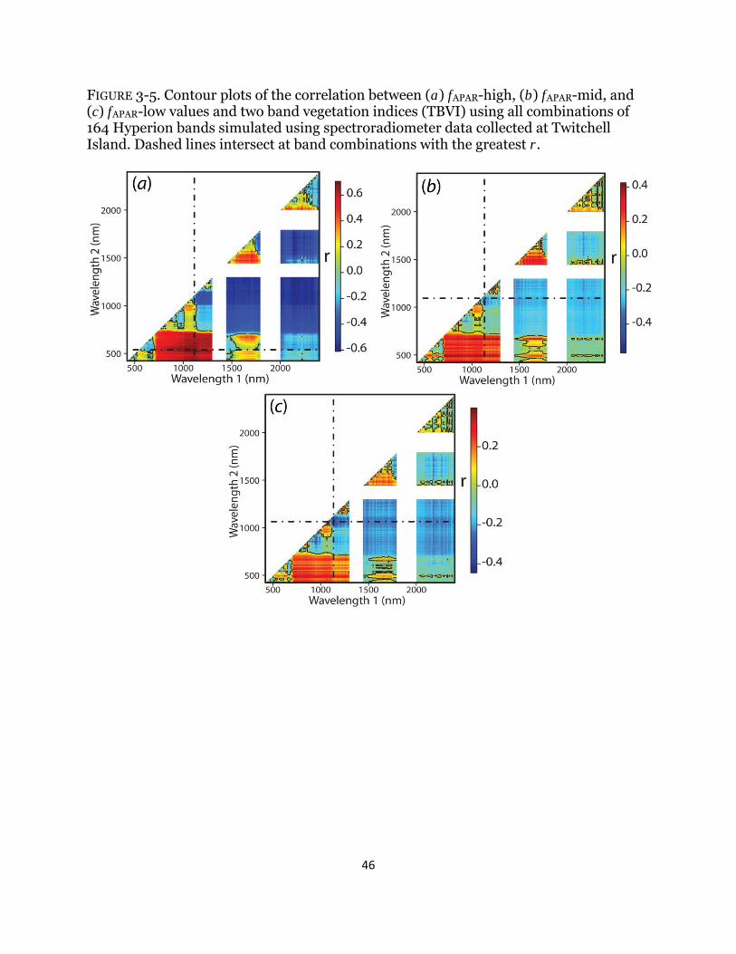
46  

FIGURE 3-5. Contour plots of the correlation between (a) fAPAR-high, (b) fAPAR-mid, and (c) fAPAR-low values and two band vegetation indices (TBVI) using all combinations of 164 Hyperion bands simulated using spectroradiometer data collected at Twitchell Island. Dashed lines intersect at band combinations with the greatest r.

 

47  

C H A P T E R F O U R

Modeling tidal wetland distribution with sea-level rise: evaluating the role of vegetation in marsh resiliency

Tidal wetlands maintain elevation with sea-level rise through feedbacks between mineral and organic matter inputs. With decreased plant production under increased inundation, projected reductions in suspended sediment concentrations, and little available upland habitat for marsh migration, multiple uncertainties exist about the resiliency of tidal wetlands with projected sea-level rise. To examine wetland resiliency, we used a rich plant productivity data set and measurements of physical properties to calibrate the Marsh Equilibrium Model (MEM), a mechanistic elevation-based soil cohort model, at four tidal wetland sites along a salinity gradient in the San Francisco Bay Estuary. Two of the wetlands have available adjacent upland habitat, and two are islands. Varying century sea-level rise rates (24, 52, 100, 165, and 180 cm) and suspended sediment concentrations (100%, 50%, and 25% of estimated current concentrations), I simulated marsh accretion across vegetated elevations for 100 years and applied the results to high resolution digital elevation models of each wetland to quantify and map changes in habitat distributions. At low levels of sea-level rise and mid and high sediment levels, all wetlands maintained vegetated elevations and shifted towards mid/high marsh elevations. As century sea-level rise was increased to 100 cm and above, wetlands began to lose elevation relative to sea level and shift to low marsh-dominated elevations, and mid/high marsh habitats were found only in former upland habitats. At the highest sea-level rise rate and lowest suspended sediment concentration, wetlands drowned, and the only vegetated areas occurred in former upland habitat. Consequently, the two island sites were less resilient than those with upland habitat, regardless of plant productivity. Future management decisions should emphasize access to upland habitat as rates of sea-level rise increase. INTRODUCTION Sea levels are projected to rise by 20 to 180 cm over the next century (IPCC 2007, Rahmstorf 2007, Vermeer and Rahmstorf 2009, Grinsted et al. 2010, National Research Council 2012) and the resiliency of tidal wetlands in the face of this sea level rise is uncertain in many respects. Historically, tidal wetlands have responded to changes in sea level through upland migration (Warren and Niering 1993, Donnelly and Bertness 2001, Elsey-Quirk et al. 2011) and via accretion through feedbacks with increased mineral (Krone 1987, Reed 1995, Marion et al. 2009) and organic matter input (Morris and Haskin 1990, Turner et al. 2000, Morris et al. 2002, Mudd et al. 2010). However, with current and projected reductions in the suspended sediment concentrations that drive mineral accretion (Syvitski et al. 2005, Cloern et al. 2011, Schoellhamer 2011) and decreased plant productivity with increased inundation (Kirwan and Guntenspergen 2012, Voss et al. 2012), it is uncertain whether wetlands can maintain vegetated

 

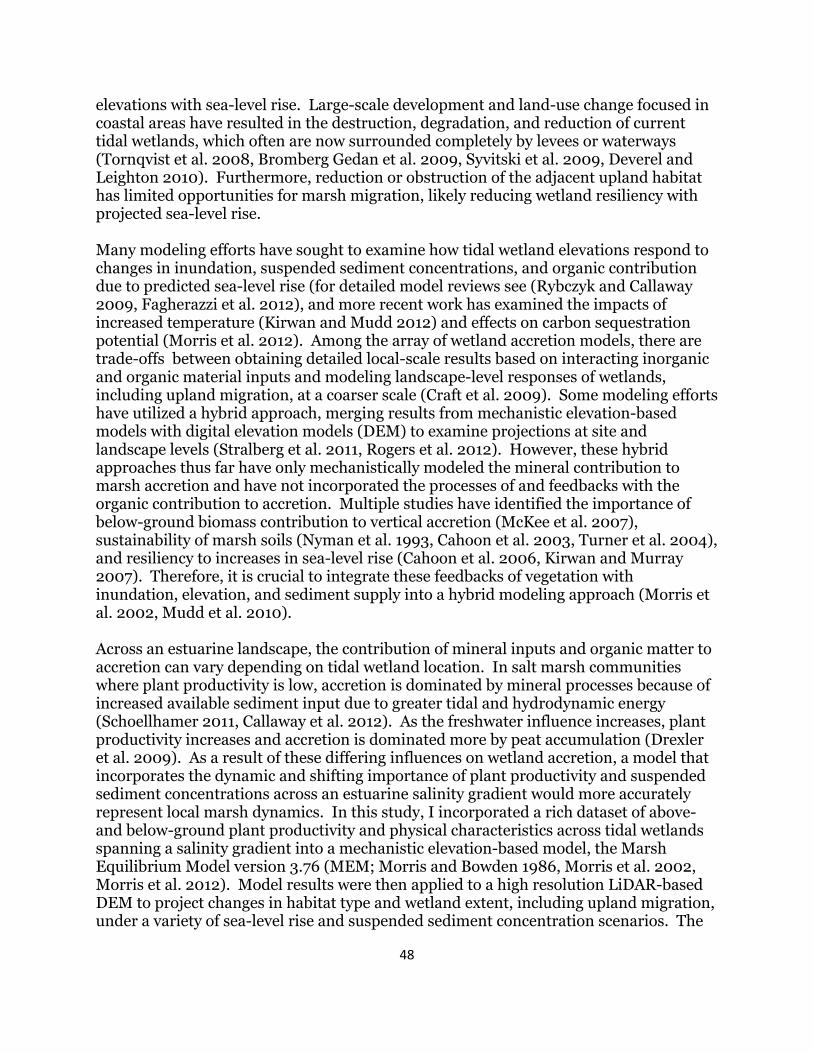
48  

elevations with sea-level rise. Large-scale development and land-use change focused in coastal areas have resulted in the destruction, degradation, and reduction of current tidal wetlands, which often are now surrounded completely by levees or waterways (Tornqvist et al. 2008, Bromberg Gedan et al. 2009, Syvitski et al. 2009, Deverel and Leighton 2010). Furthermore, reduction or obstruction of the adjacent upland habitat has limited opportunities for marsh migration, likely reducing wetland resiliency with projected sea-level rise. Many modeling efforts have sought to examine how tidal wetland elevations respond to changes in inundation, suspended sediment concentrations, and organic contribution due to predicted sea-level rise (for detailed model reviews see (Rybczyk and Callaway 2009, Fagherazzi et al. 2012), and more recent work has examined the impacts of increased temperature (Kirwan and Mudd 2012) and effects on carbon sequestration potential (Morris et al. 2012). Among the array of wetland accretion models, there are trade-offs between obtaining detailed local-scale results based on interacting inorganic and organic material inputs and modeling landscape-level responses of wetlands, including upland migration, at a coarser scale (Craft et al. 2009). Some modeling efforts have utilized a hybrid approach, merging results from mechanistic elevation-based models with digital elevation models (DEM) to examine projections at site and landscape levels (Stralberg et al. 2011, Rogers et al. 2012). However, these hybrid approaches thus far have only mechanistically modeled the mineral contribution to marsh accretion and have not incorporated the processes of and feedbacks with the organic contribution to accretion. Multiple studies have identified the importance of below-ground biomass contribution to vertical accretion (McKee et al. 2007), sustainability of marsh soils (Nyman et al. 1993, Cahoon et al. 2003, Turner et al. 2004), and resiliency to increases in sea-level rise (Cahoon et al. 2006, Kirwan and Murray 2007). Therefore, it is crucial to integrate these feedbacks of vegetation with inundation, elevation, and sediment supply into a hybrid modeling approach (Morris et al. 2002, Mudd et al. 2010). Across an estuarine landscape, the contribution of mineral inputs and organic matter to accretion can vary depending on tidal wetland location. In salt marsh communities where plant productivity is low, accretion is dominated by mineral processes because of increased available sediment input due to greater tidal and hydrodynamic energy (Schoellhamer 2011, Callaway et al. 2012). As the freshwater influence increases, plant productivity increases and accretion is dominated more by peat accumulation (Drexler et al. 2009). As a result of these differing influences on wetland accretion, a model that incorporates the dynamic and shifting importance of plant productivity and suspended sediment concentrations across an estuarine salinity gradient would more accurately represent local marsh dynamics. In this study, I incorporated a rich dataset of above- and below-ground plant productivity and physical characteristics across tidal wetlands spanning a salinity gradient into a mechanistic elevation-based model, the Marsh Equilibrium Model version 3.76 (MEM; Morris and Bowden 1986, Morris et al. 2002, Morris et al. 2012). Model results were then applied to a high resolution LiDAR-based DEM to project changes in habitat type and wetland extent, including upland migration, under a variety of sea-level rise and suspended sediment concentration scenarios. The

 

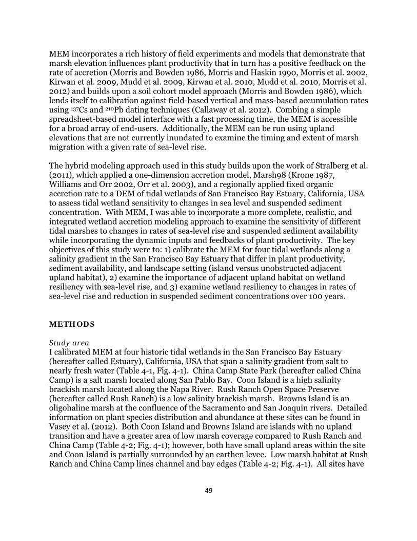
49  

MEM incorporates a rich history of field experiments and models that demonstrate that marsh elevation influences plant productivity that in turn has a positive feedback on the rate of accretion (Morris and Bowden 1986, Morris and Haskin 1990, Morris et al. 2002, Kirwan et al. 2009, Mudd et al. 2009, Kirwan et al. 2010, Mudd et al. 2010, Morris et al. 2012) and builds upon a soil cohort model approach (Morris and Bowden 1986), which lends itself to calibration against field-based vertical and mass-based accumulation rates using 137Cs and 210Pb dating techniques (Callaway et al. 2012). Combing a simple spreadsheet-based model interface with a fast processing time, the MEM is accessible for a broad array of end-users. Additionally, the MEM can be run using upland elevations that are not currently inundated to examine the timing and extent of marsh migration with a given rate of sea-level rise. The hybrid modeling approach used in this study builds upon the work of Stralberg et al. (2011), which applied a one-dimension accretion model, Marsh98 (Krone 1987, Williams and Orr 2002, Orr et al. 2003), and a regionally applied fixed organic accretion rate to a DEM of tidal wetlands of San Francisco Bay Estuary, California, USA to assess tidal wetland sensitivity to changes in sea level and suspended sediment concentration. With MEM, I was able to incorporate a more complete, realistic, and integrated wetland accretion modeling approach to examine the sensitivity of different tidal marshes to changes in rates of sea-level rise and suspended sediment availability while incorporating the dynamic inputs and feedbacks of plant productivity. The key objectives of this study were to: 1) calibrate the MEM for four tidal wetlands along a salinity gradient in the San Francisco Bay Estuary that differ in plant productivity, sediment availability, and landscape setting (island versus unobstructed adjacent upland habitat), 2) examine the importance of adjacent upland habitat on wetland resiliency with sea-level rise, and 3) examine wetland resiliency to changes in rates of sea-level rise and reduction in suspended sediment concentrations over 100 years. METHODS Study area I calibrated MEM at four historic tidal wetlands in the San Francisco Bay Estuary (hereafter called Estuary), California, USA that span a salinity gradient from salt to nearly fresh water (Table 4-1, Fig. 4-1). China Camp State Park (hereafter called China Camp) is a salt marsh located along San Pablo Bay. Coon Island is a high salinity brackish marsh located along the Napa River. Rush Ranch Open Space Preserve (hereafter called Rush Ranch) is a low salinity brackish marsh. Browns Island is an oligohaline marsh at the confluence of the Sacramento and San Joaquin rivers. Detailed information on plant species distribution and abundance at these sites can be found in Vasey et al. (2012). Both Coon Island and Browns Island are islands with no upland transition and have a greater area of low marsh coverage compared to Rush Ranch and China Camp (Table 4-2; Fig. 4-1); however, both have small upland areas within the site and Coon Island is partially surrounded by an earthen levee. Low marsh habitat at Rush Ranch and China Camp lines channel and bay edges (Table 4-2; Fig. 4-1). All sites have

 

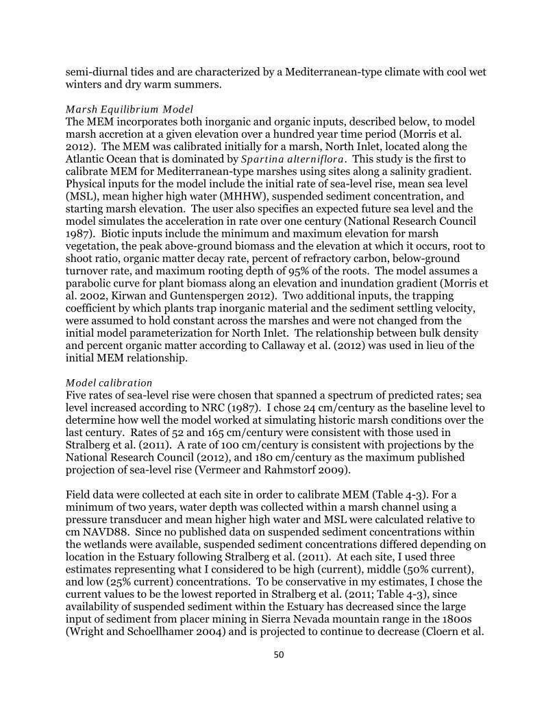
50  

semi-diurnal tides and are characterized by a Mediterranean-type climate with cool wet winters and dry warm summers. Marsh Equilibrium Model The MEM incorporates both inorganic and organic inputs, described below, to model marsh accretion at a given elevation over a hundred year time period (Morris et al. 2012). The MEM was calibrated initially for a marsh, North Inlet, located along the Atlantic Ocean that is dominated by Spartina alterniflora. This study is the first to calibrate MEM for Mediterranean-type marshes using sites along a salinity gradient. Physical inputs for the model include the initial rate of sea-level rise, mean sea level (MSL), mean higher high water (MHHW), suspended sediment concentration, and starting marsh elevation. The user also specifies an expected future sea level and the model simulates the acceleration in rate over one century (National Research Council 1987). Biotic inputs include the minimum and maximum elevation for marsh vegetation, the peak above-ground biomass and the elevation at which it occurs, root to shoot ratio, organic matter decay rate, percent of refractory carbon, below-ground turnover rate, and maximum rooting depth of 95% of the roots. The model assumes a parabolic curve for plant biomass along an elevation and inundation gradient (Morris et al. 2002, Kirwan and Guntenspergen 2012). Two additional inputs, the trapping coefficient by which plants trap inorganic material and the sediment settling velocity, were assumed to hold constant across the marshes and were not changed from the initial model parameterization for North Inlet. The relationship between bulk density and percent organic matter according to Callaway et al. (2012) was used in lieu of the initial MEM relationship. Model calibration Five rates of sea-level rise were chosen that spanned a spectrum of predicted rates; sea level increased according to NRC (1987). I chose 24 cm/century as the baseline level to determine how well the model worked at simulating historic marsh conditions over the last century. Rates of 52 and 165 cm/century were consistent with those used in Stralberg et al. (2011). A rate of 100 cm/century is consistent with projections by the National Research Council (2012), and 180 cm/century as the maximum published projection of sea-level rise (Vermeer and Rahmstorf 2009). Field data were collected at each site in order to calibrate MEM (Table 4-3). For a minimum of two years, water depth was collected within a marsh channel using a pressure transducer and mean higher high water and MSL were calculated relative to cm NAVD88. Since no published data on suspended sediment concentrations within the wetlands were available, suspended sediment concentrations differed depending on location in the Estuary following Stralberg et al. (2011). At each site, I used three estimates representing what I considered to be high (current), middle (50% current), and low (25% current) concentrations. To be conservative in my estimates, I chose the current values to be the lowest reported in Stralberg et al. (2011; Table 4-3), since availability of suspended sediment within the Estuary has decreased since the large input of sediment from placer mining in Sierra Nevada mountain range in the 1800s (Wright and Schoellhamer 2004) and is projected to continue to decrease (Cloern et al.

 

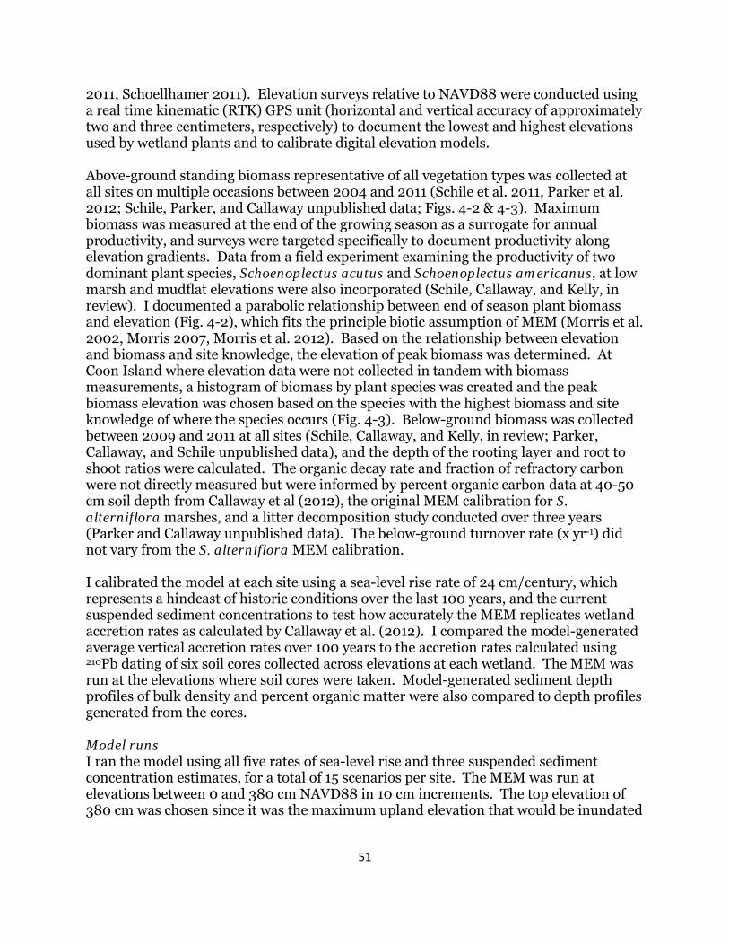
51  

2011, Schoellhamer 2011). Elevation surveys relative to NAVD88 were conducted using a real time kinematic (RTK) GPS unit (horizontal and vertical accuracy of approximately two and three centimeters, respectively) to document the lowest and highest elevations used by wetland plants and to calibrate digital elevation models. Above-ground standing biomass representative of all vegetation types was collected at all sites on multiple occasions between 2004 and 2011 (Schile et al. 2011, Parker et al. 2012; Schile, Parker, and Callaway unpublished data; Figs. 4-2 & 4-3). Maximum biomass was measured at the end of the growing season as a surrogate for annual productivity, and surveys were targeted specifically to document productivity along elevation gradients. Data from a field experiment examining the productivity of two dominant plant species, Schoenoplectus acutus and Schoenoplectus americanus, at low marsh and mudflat elevations were also incorporated (Schile, Callaway, and Kelly, in review). I documented a parabolic relationship between end of season plant biomass and elevation (Fig. 4-2), which fits the principle biotic assumption of MEM (Morris et al. 2002, Morris 2007, Morris et al. 2012). Based on the relationship between elevation and biomass and site knowledge, the elevation of peak biomass was determined. At Coon Island where elevation data were not collected in tandem with biomass measurements, a histogram of biomass by plant species was created and the peak biomass elevation was chosen based on the species with the highest biomass and site knowledge of where the species occurs (Fig. 4-3). Below-ground biomass was collected between 2009 and 2011 at all sites (Schile, Callaway, and Kelly, in review; Parker, Callaway, and Schile unpublished data), and the depth of the rooting layer and root to shoot ratios were calculated. The organic decay rate and fraction of refractory carbon were not directly measured but were informed by percent organic carbon data at 40-50 cm soil depth from Callaway et al (2012), the original MEM calibration for S. alterniflora marshes, and a litter decomposition study conducted over three years (Parker and Callaway unpublished data). The below-ground turnover rate (x yr-1) did not vary from the S. alterniflora MEM calibration. I calibrated the model at each site using a sea-level rise rate of 24 cm/century, which represents a hindcast of historic conditions over the last 100 years, and the current suspended sediment concentrations to test how accurately the MEM replicates wetland accretion rates as calculated by Callaway et al. (2012). I compared the model-generated average vertical accretion rates over 100 years to the accretion rates calculated using 210Pb dating of six soil cores collected across elevations at each wetland. The MEM was run at the elevations where soil cores were taken. Model-generated sediment depth profiles of bulk density and percent organic matter were also compared to depth profiles generated from the cores. Model runs I ran the model using all five rates of sea-level rise and three suspended sediment concentration estimates, for a total of 15 scenarios per site. The MEM was run at elevations between 0 and 380 cm NAVD88 in 10 cm increments. The top elevation of 380 cm was chosen since it was the maximum upland elevation that would be inundated

 

52  

by a 180 cm increase in sea level. Results were interpolated evenly for every centimeter of elevation in between each model run. Spatial Analyses A DEM for each site was created using the 2009-2011 California Coastal Conservancy’s Coastal LiDAR Project data (Department of Commerce et al. 2012), which is a more recent DEM that what was used in Stralberg et al (2011). The DEM was generated at a 1 m2 spatial resolution with the vertical datum NAVD88 GEOID09 model for orthometric heights. To account for the effects of vegetation on DEMs created using LiDAR data (Hladik and Alber 2012), elevations were adjusted between 0 and 70 cm lower when necessary based on comparison with comprehensive RTK elevation surveys across all sites, vegetation maps (Tuxen et al. 2011), and knowledge of vegetation distribution, height of live vegetation, and height of dense standing dead vegetation. Elevations were clipped to 390 cm NAVD and lower to restrict the DEM to elevations relevant for the analysis, since both China Camp and Rush Ranch have large areas of unobstructed adjacent upland habitat that extends well above marsh elevations (Table 4-2). All values were rounded up to the nearest whole cm. A mask was created in ArcMap 10 (ESRI Inc. 2010) to remove tidal channels from the analysis since MEM works most accurately when applied to areas with laminar, not turbulent, flow (Morris et al. 2012). For each site beginning with the initial elevation at time zero, modeled elevations were compiled for runs that were 20, 50, 70 and 100 years into the future, corresponding to years 2010, 2030, 2060, 2080, and 2110, respectively. Using ArcMap Model Builder (ESRI Inc. 2010), modeled elevations from each time period were applied to the DEM and then transformed relative to the corresponding MSL using the equation: (marsh elevation – MSL) / (MHHW – MSL). I assumed that there was no change in the relationship between MSL and MHHW over time. In order to classify the DEM into marsh habitat type, I determined cut-off elevations for transitions between mudflat, low marsh, mid/high marsh, and upland habitat based on elevation surveys of current distributions of each habitat type relative to MSL (Table 4-4; see Fig. 4-1 for starting conditions). I chose not to differentiate between mid and high marsh habitat since it does not always correspond with elevation alone. The area of each habitat type was calculated for every model scenario and time period. At the site level, I evaluated the stability of the distributions of current wetland habitats over time using the 24 cm/century sea-level rise and current suspended sediment concentrations as a way of assessing model calibration/accuracy at that spatial scale. I assumed that marsh conditions have been relatively stable over the last 100 years and, as such, that the model results will show little change in habitat distribution with the 24 cm/century rise. RESULTS Under the mid and high suspended sediment concentrations, all marshes responded similarly under the two lower (24 and 52 cm/century) and two higher (165 and 180

 

53  

cm/century) SLR scenarios, respectively, and the 100 cm/century SLR scenario had intermediate results (Figs. 4 & 5). As such, I chose to map changes in the spatial distribution of marsh habitats after 100 years for the 52, 100, and 180 cm/century SLR for the low and high suspended sediment concentrations (Figs. 4-6 – 4-9). Model Calibration Model-generated output for the 24 cm/century sea-level rise scenario simulating historic conditions were consistently within the range of soil core-based accretion rates and bulk density, and percent organic matter depth profiles data (Table 4-5 & Fig. 4-10). Additionally, marsh habitat distributions changed little over 100 years with both the mid and high suspended sediment concentrations (Fig 4-11). Mid and High Suspended Sediment Concentrations With increasing rates of SLR, there was a trend of conversion from mid/high marsh elevations to low marsh elevations across all sites, and the timing of the conversion occurred sooner as SLR increased (Figs. 4-4 & 4-5). In the 52 cm/century SLR scenario, low marsh elevations tended to accrete to mid/high marsh elevations, covering between 74 and 99% of the marsh after 100 years (Figs. 4-4 & 4-5). With 100 cm/century SLR, elevations at all sites were indicative of low marsh habitat, covering roughly 90% after 100 years (Figs. 4-4 & 4-5). Under the 165 and 180 cm/century SLR scenarios, all marshes showed signs of losing elevation relative to sea level, most significantly in the island sites that had lower initial starting elevations. At China Camp and Rush Ranch, the dominant marsh elevations shifted from mid/high marsh to low marsh conditions after 70 years (Figs. 4-4a & 4-5a) whereas elevations at the two island sites, Coon and Browns Islands, shifted after 50 years (Figs. 4-4b & 4-5b). After 100 years, Browns Island showed marked signs of drowning, as evidenced by the predominance of unvegetated habitat (97%) at the mid suspended sediment concentration (Figs. 4-5b & 4-9e). Less than 1% of mid/high marsh elevations remained at the two island sites after 100 years (Figs. 4-4b, 4-5b, 4-7e, & 4-9e) and the only remaining mid/high marsh habitat at China Camp and Rush Ranch were in areas that were formerly upland habitat (Figs. 4-6e & 4-8e). Low Suspended Sediment Concentrations Under the lowest suspended sediment concentrations, differences among sites were more exaggerated. Under the 24 and 52 cm/century SLR scenarios, China Camp exhibited little response to SLR and resembled current marsh conditions even after 100 years (Figs. 4-1 & 4-6b). Low marsh elevations dominated after 70 years under the 100 cm/century SLR scenario and after 50 years under both the 165 and 180 cm/century scenarios. Eighty eight percent of China Camp was at elevations indicative of unvegetated habitat with 180 cm of SLR after 100 years (Figs. 4-4a & 4-6f); the only vegetated areas occurred in formerly upland habitat (Fig. 4-6f). Coon Island began to shift to a low marsh-dominated system after 70 years in the 52 cm/century SLR scenario and after 50 years in the 100 cm/century scenario (Fig. 4-4b). Marsh drowning began to occur after 100 years with the 100 cm SLR scenario (Fig. 4-7d), and was dominated by unvegetated elevations after 70 years at the higher two SLR rates (Fig. 4-4b); only a

 

54  

small strip of vegetation remained along a levee after 100 years with 180cm SLR (Fig. 4-7f). At the two lower salinity sites that had overall higher plant productivity and lower suspended sediment concentrations, wetlands failed to keep pace with sea-level rise as rates increased and began to drown. Rush Ranch marsh habitat changed little over 100 years under the 52 cm/century SLR scenario (Figs. 4-5a & 4-8b). After 100 years for the 100 cm/century sea-level rise rate, the marsh was dominated by low marsh elevations and mid/high marsh habitat was located only in former upland areas (Figs. 4-5a & 4-8d). Low marsh dominance occurred after 70 years under the highest two SLR scenarios and marked wetland drowning occurred after 100 years; the majority of vegetated habitat occurred in former upland areas (Figs. 4-5a & 4-7f). Browns Island low marsh elevations increased to 90% cover after 100 years in the 52 cm SLR scenario (Figs. 4-5b & 4-8b) and dominated the landscape after 70 years under the 100 cm/century SLR scenario (Fig. 4b). Less than 1% of mid/high marsh habitat remained after 50 years in the 165 and 180 cm/century scenarios (Fig. 4-5b) and 98% of Browns Island was unvegetated after 100 years with a 180 cm SLR (Fig. 4-9f). DISCUSSION Effects of plant productivity on marsh resiliency Across four sites that differ in plant productivity, salinity, and suspended sediment concentrations, I was able to successfully calibrate MEM and run a variety of sea-level rise and suspended sediment concentration scenarios to assess marsh resiliency over 100 years. I demonstrated a parabolic relationship with productivity along an elevation gradient, which is a key assumption for successful calibration of MEM (Morris et al. 2002). In this study, wetland resiliency to increased sea-level rise after 100 years was greater when both the organic and mineral contributions to accretion were mechanistically modeled compared to a study where only the mineral contributions were mechanistically modeled (see Stralberg et al. 2011 and http://data.prbo.org/apps /sfbslr/ for maps of results). Although it is difficult to make direct model comparisons between Stralberg et al. (2011) and this current study to explore model differences due to use of different DEMs, I can examine the influence and importance of plant productivity in accretion with results from MEM. Using a suspended sediment concentration of 25 mg/L, a concentration that was modeled across all sites, and a 180 cm/century of SLR, the brackish wetlands with the higher productivity largely maintained vegetated elevations on the marsh plain after 100 years (Figs. 4-9f & 4-12) compared to the salt marsh sites with lower plant productivity (Figs 4-6f & 4-7f), which had drowned after 100 years. In order to apply MEM successfully across an estuary, data on plant productivity need to be collected at multiple marsh locations to account for effects of salinity on production. Often, this is a labor intensive practice, particularly for measurements of below-ground biomass, but it is crucial in order to more accurately model marsh accretion (Kirwan and Murray 2007, Mudd et al. 2010), particularly in freshwater sites with low soil bulk

 

55  

density (Kirwan and Mudd 2012). Intensive field data collection and model calibration at a few sites that are characteristic of a suite of wetlands within that salinity range, as demonstrated in this study, allows for the app1ication of the model at the estuary level. I chose to only focus on four sites for the sea-level rise scenarios to examine the model and mapped results more critically. Effect of landscape position and elevation on marsh resiliency A striking difference across sites was the availability of adjacent upland habitat for wetland migration. Under the highest sea-level rise scenarios, mid/high marsh elevations, and in some cases the only vegetated marsh habitat for the entire marsh, were entirely restricted to what was initially upland habitat (Figs. 4-6f, 4-7f, & 4-9f). The island sites that lacked extensive upland habitat either had no mid/high marsh habitat after 100 years or were almost entirely drowned. As such, these island sites are less resilient to loss under sea-level rise, regardless of plant productivity and suspended sediment concentration. Initial marsh plain elevation also played a role in wetland resiliency with increased rates of sea-level rise. Both Coon and Browns Islands had starting elevations that, on average, were lower than the other sites and had a broader coverage of low marsh habitat (Table 4-2; Fig. 4-1). Initially, this translated into an increase in mid/high marsh elevation at the expense of low marsh elevations across all sea-level rise scenarios because of accelerated accretion rates to equilibrate with sea-level rise, which has been documented in other modeling studies (Morris et al. 2002, Mudd et al. 2009, Kirwan and Mudd 2012) and field studies (Nyman et al. 2006, McKee et al. 2007). However, the increase in sea level resulted in the inability for the wetlands to keep pace with sea-level rise and the elevation shifted towards low marsh elevations again. This change in elevation over time was not apparent China Camp and Rush Ranch since there was minimal low marsh coverage under initial conditions (Fig. 4-1). Additionally, both of these upland-bordering sites have broad marsh plains with relatively uniform elevations and large-scale shifts in habitat type occurred rather abruptly when the threshold points were crossed. Ultimately, the starting marsh elevation affected the initial rate of habitat conversion but the net result after 100 years was similar across sites. Effect of suspended sediment concentration on marsh resiliency Accretion rates could not keep pace with high rates of sea-level rise when suspended sediment concentrations were low, a finding supported by other models (Kirwan et al. 2010). A reduction in suspended sediment concentrations at the saltier sites, which have lower plant productivity, resulted in an inability of the wetland to maintain current elevations with sea-level rise; this effect was not as marked in the less saline sites. These results are corroborated by field studies that documented higher bulk density values in salt marshes; they require more mineral input to maintain elevations relative to sea-level rise (Nyman et al. 1990, Thom 1992). A reduction in suspended sediment in the salt marshes resulted in an earlier conversion to low marsh elevations under the 100 cm/century SLR scenario and almost complete marsh drowning under the 180 cm/century SLR scenario. Under the 24, 52, and 100 cm/century SLR scenarios, a reduction in suspended sediment did not result in a large difference in modeled results

 

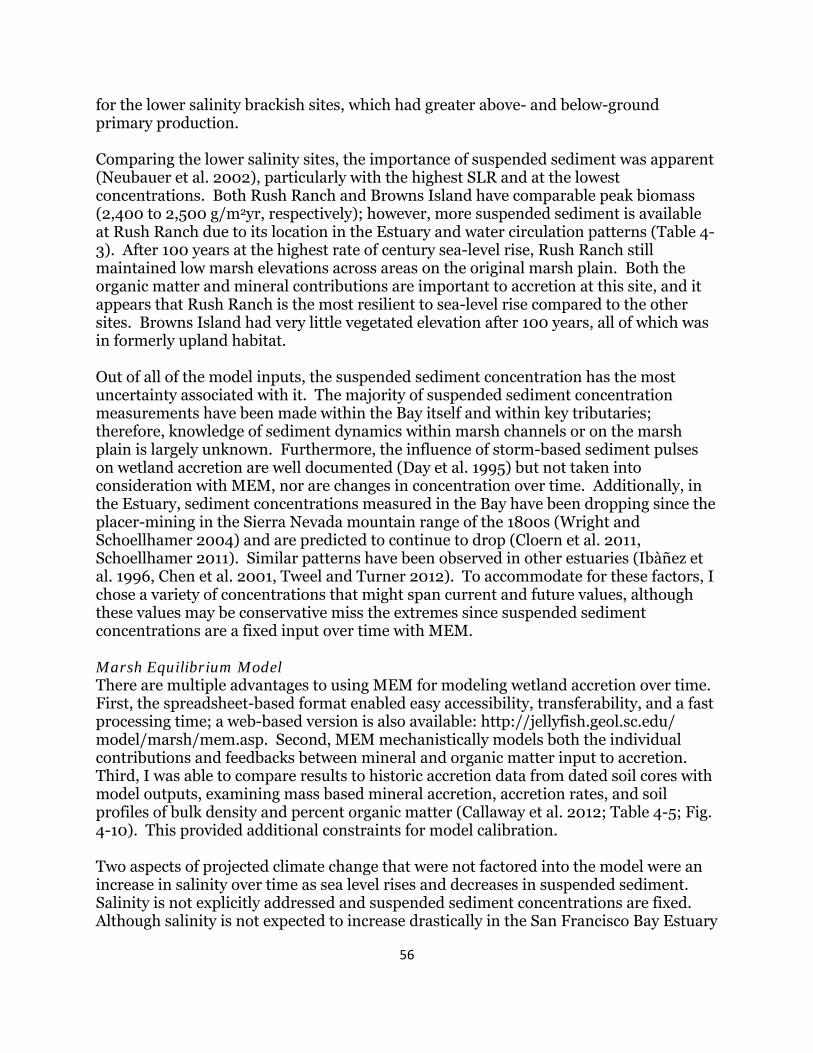
56  

for the lower salinity brackish sites, which had greater above- and below-ground primary production. Comparing the lower salinity sites, the importance of suspended sediment was apparent (Neubauer et al. 2002), particularly with the highest SLR and at the lowest concentrations. Both Rush Ranch and Browns Island have comparable peak biomass (2,400 to 2,500 g/m2yr, respectively); however, more suspended sediment is available at Rush Ranch due to its location in the Estuary and water circulation patterns (Table 4-3). After 100 years at the highest rate of century sea-level rise, Rush Ranch still maintained low marsh elevations across areas on the original marsh plain. Both the organic matter and mineral contributions are important to accretion at this site, and it appears that Rush Ranch is the most resilient to sea-level rise compared to the other sites. Browns Island had very little vegetated elevation after 100 years, all of which was in formerly upland habitat. Out of all of the model inputs, the suspended sediment concentration has the most uncertainty associated with it. The majority of suspended sediment concentration measurements have been made within the Bay itself and within key tributaries; therefore, knowledge of sediment dynamics within marsh channels or on the marsh plain is largely unknown. Furthermore, the influence of storm-based sediment pulses on wetland accretion are well documented (Day et al. 1995) but not taken into consideration with MEM, nor are changes in concentration over time. Additionally, in the Estuary, sediment concentrations measured in the Bay have been dropping since the placer-mining in the Sierra Nevada mountain range of the 1800s (Wright and Schoellhamer 2004) and are predicted to continue to drop (Cloern et al. 2011, Schoellhamer 2011). Similar patterns have been observed in other estuaries (Ibàñez et al. 1996, Chen et al. 2001, Tweel and Turner 2012). To accommodate for these factors, I chose a variety of concentrations that might span current and future values, although these values may be conservative miss the extremes since suspended sediment concentrations are a fixed input over time with MEM. Marsh Equilibrium Model There are multiple advantages to using MEM for modeling wetland accretion over time. First, the spreadsheet-based format enabled easy accessibility, transferability, and a fast processing time; a web-based version is also available: http://jellyfish.geol.sc.edu/ model/marsh/mem.asp. Second, MEM mechanistically models both the individual contributions and feedbacks between mineral and organic matter input to accretion. Third, I was able to compare results to historic accretion data from dated soil cores with model outputs, examining mass based mineral accretion, accretion rates, and soil profiles of bulk density and percent organic matter (Callaway et al. 2012; Table 4-5; Fig. 4-10). This provided additional constraints for model calibration. Two aspects of projected climate change that were not factored into the model were an increase in salinity over time as sea level rises and decreases in suspended sediment. Salinity is not explicitly addressed and suspended sediment concentrations are fixed. Although salinity is not expected to increase drastically in the San Francisco Bay Estuary

 

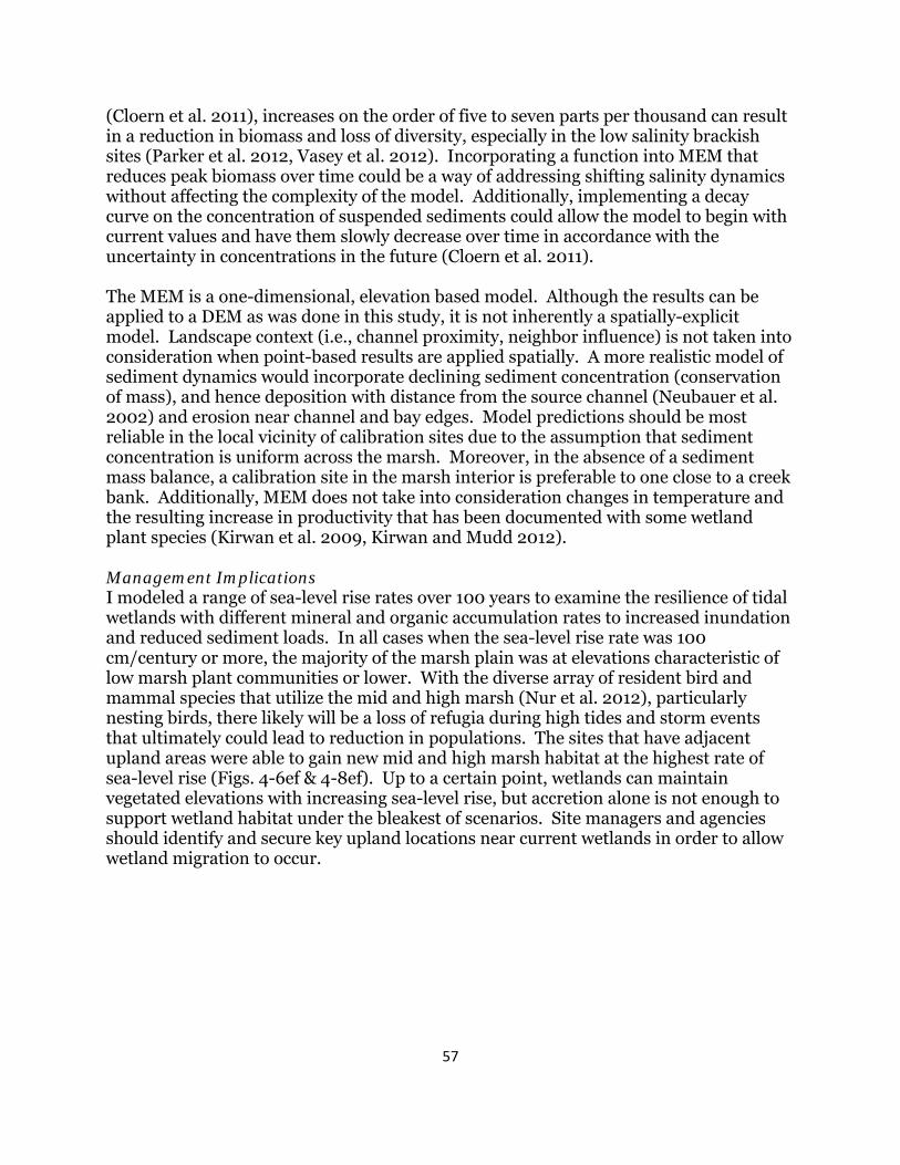
57  

(Cloern et al. 2011), increases on the order of five to seven parts per thousand can result in a reduction in biomass and loss of diversity, especially in the low salinity brackish sites (Parker et al. 2012, Vasey et al. 2012). Incorporating a function into MEM that reduces peak biomass over time could be a way of addressing shifting salinity dynamics without affecting the complexity of the model. Additionally, implementing a decay curve on the concentration of suspended sediments could allow the model to begin with current values and have them slowly decrease over time in accordance with the uncertainty in concentrations in the future (Cloern et al. 2011). The MEM is a one-dimensional, elevation based model. Although the results can be applied to a DEM as was done in this study, it is not inherently a spatially-explicit model. Landscape context (i.e., channel proximity, neighbor influence) is not taken into consideration when point-based results are applied spatially. A more realistic model of sediment dynamics would incorporate declining sediment concentration (conservation of mass), and hence deposition with distance from the source channel (Neubauer et al. 2002) and erosion near channel and bay edges. Model predictions should be most reliable in the local vicinity of calibration sites due to the assumption that sediment concentration is uniform across the marsh. Moreover, in the absence of a sediment mass balance, a calibration site in the marsh interior is preferable to one close to a creek bank. Additionally, MEM does not take into consideration changes in temperature and the resulting increase in productivity that has been documented with some wetland plant species (Kirwan et al. 2009, Kirwan and Mudd 2012). Management Implications I modeled a range of sea-level rise rates over 100 years to examine the resilience of tidal wetlands with different mineral and organic accumulation rates to increased inundation and reduced sediment loads. In all cases when the sea-level rise rate was 100 cm/century or more, the majority of the marsh plain was at elevations characteristic of low marsh plant communities or lower. With the diverse array of resident bird and mammal species that utilize the mid and high marsh (Nur et al. 2012), particularly nesting birds, there likely will be a loss of refugia during high tides and storm events that ultimately could lead to reduction in populations. The sites that have adjacent upland areas were able to gain new mid and high marsh habitat at the highest rate of sea-level rise (Figs. 4-6ef & 4-8ef). Up to a certain point, wetlands can maintain vegetated elevations with increasing sea-level rise, but accretion alone is not enough to support wetland habitat under the bleakest of scenarios. Site managers and agencies should identify and secure key upland locations near current wetlands in order to allow wetland migration to occur.

 

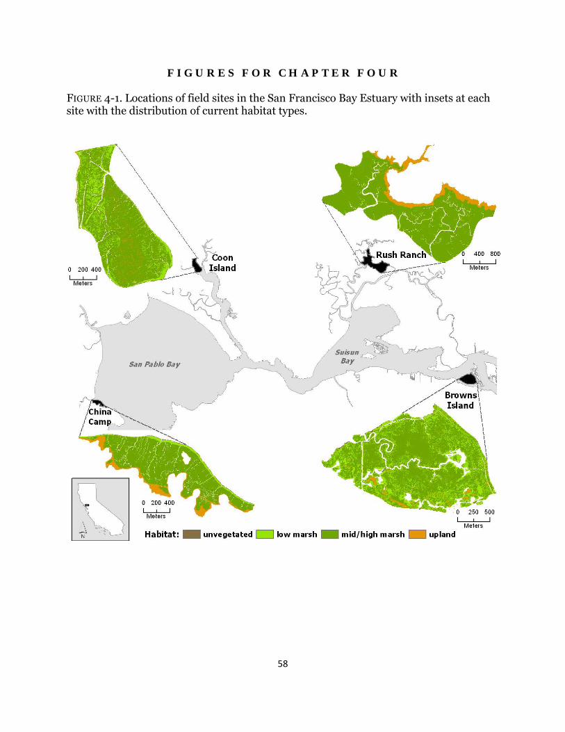
58  

F I G U R E S F O R C H A P T E R F O U R

FIGURE 4-1. Locations of field sites in the San Francisco Bay Estuary with insets at each site with the distribution of current habitat types.

 

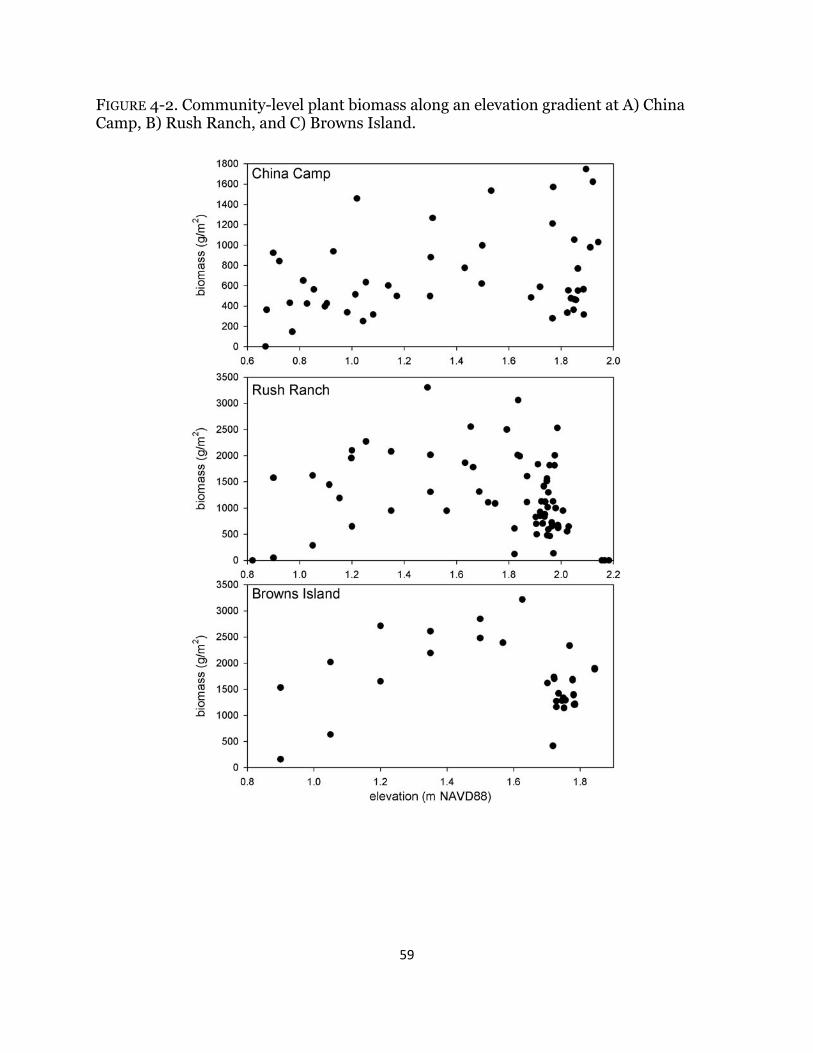
59  

FIGURE 4-2. Community-level plant biomass along an elevation gradient at A) China Camp, B) Rush Ranch, and C) Browns Island.

 

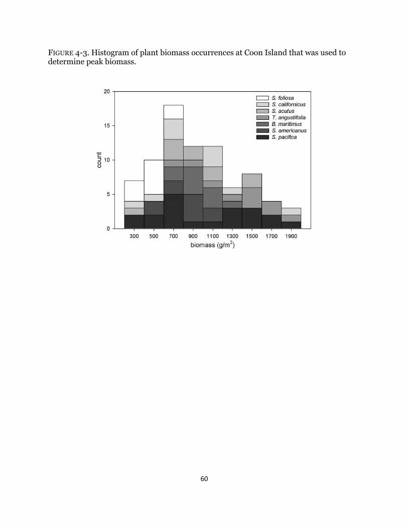
60  

FIGURE 4-3. Histogram of plant biomass occurrences at Coon Island that was used to determine peak biomass.

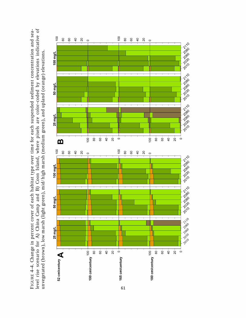
     61FIG

UR

E 4

-4.

Ch

ange

in

per

cen

t co

ver

of e

ach

hab

itat

typ

e ov

er t

ime

for

each

su

spen

ded

sed

imen

t co

nce

ntr

atio

n a

nd

sea

-le

vel

rise

sce

nar

io f

or A

) C

hin

a C

amp

an

d B

) C

oon

Isl

and

, w

her

e p

ixel

s ar

e co

lor-

cod

ed b

y el

evat

ion

s in

dic

ativ

e of

u

nve

geta

ted

(br

own

), lo

w m

arsh

(li

ght

gree

n),

mid

/hig

h m

arsh

(m

ediu

m g

reen

), a

nd

up

lan

d (

oran

ge)

elev

atio

ns.

 

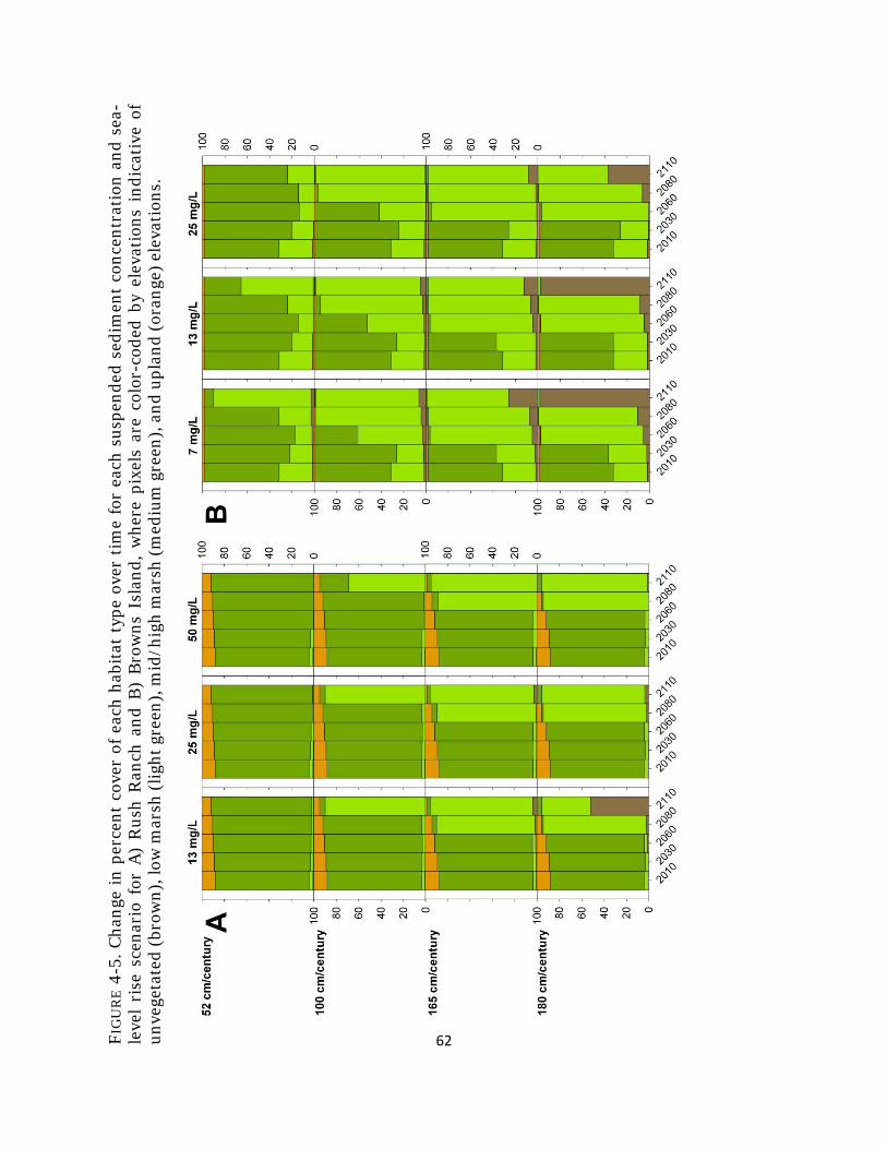
     62FIG

UR

E 4

-5.

Ch

ange

in

per

cen

t co

ver

of e

ach

hab

itat

typ

e ov

er t

ime

for

each

su

spen

ded

sed

imen

t co

nce

ntr

atio

n a

nd

sea

-le

vel

rise

sce

nar

io f

or A

) R

ush

Ran

ch a

nd

B)

Bro

wn

s Is

lan

d,

wh

ere

pix

els

are

colo

r-co

ded

by

elev

atio

ns

ind

icat

ive

of

un

vege

tate

d (

brow

n),

low

mar

sh (

ligh

t gr

een

), m

id/h

igh

mar

sh (

med

ium

gre

en),

an

d u

pla

nd

(or

ange

) el

evat

ion

s.

 

 

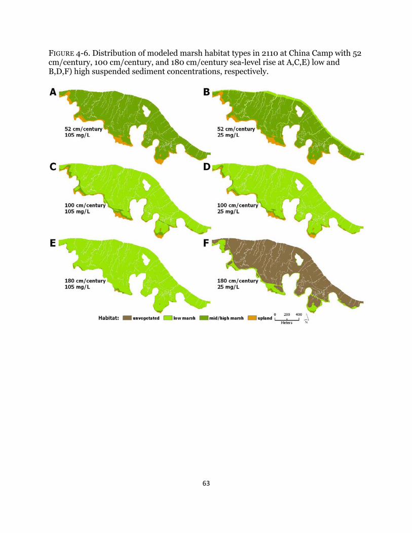
63  

FIGURE 4-6. Distribution of modeled marsh habitat types in 2110 at China Camp with 52 cm/century, 100 cm/century, and 180 cm/century sea-level rise at A,C,E) low and B,D,F) high suspended sediment concentrations, respectively.

 

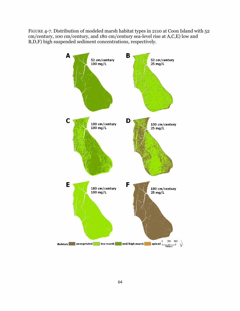
64  

FIGURE 4-7. Distribution of modeled marsh habitat types in 2110 at Coon Island with 52 cm/century, 100 cm/century, and 180 cm/century sea-level rise at A,C,E) low and B,D,F) high suspended sediment concentrations, respectively.

 

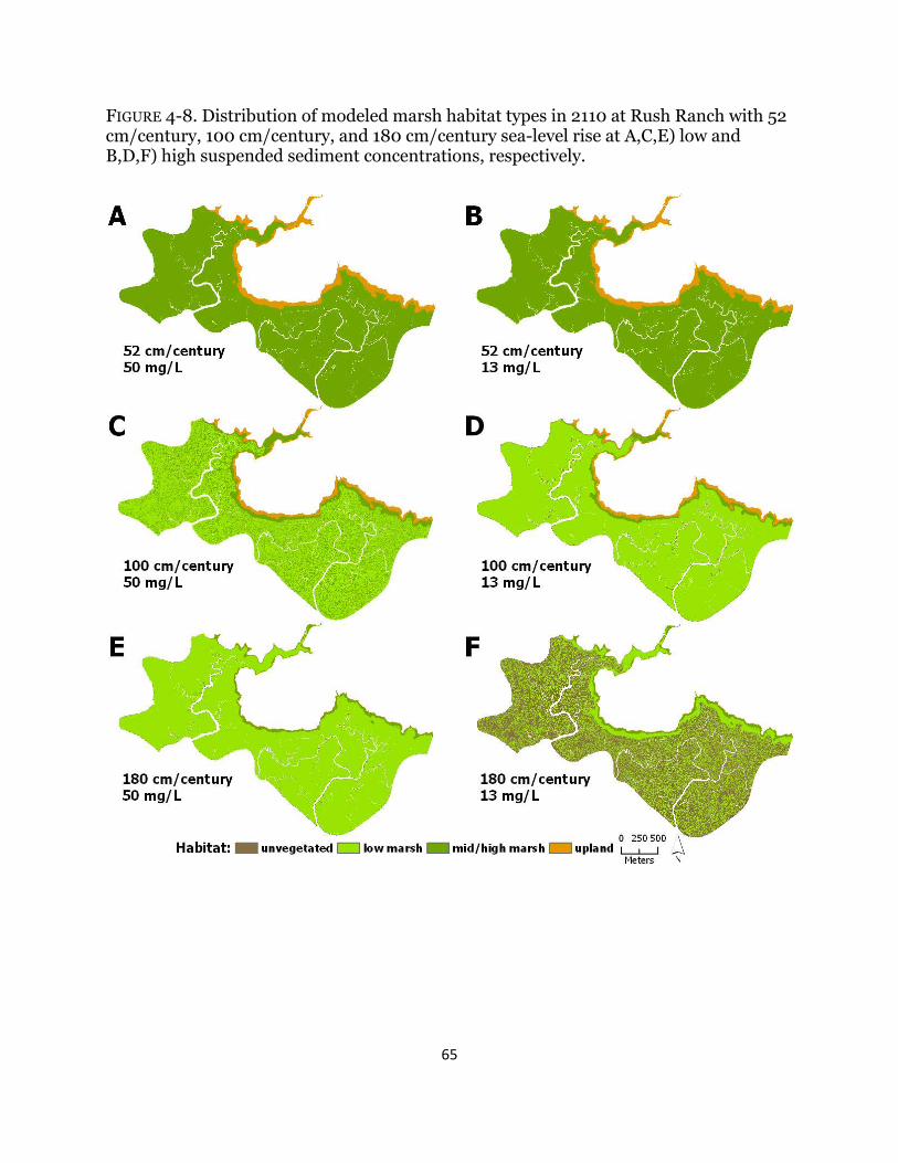
65  

FIGURE 4-8. Distribution of modeled marsh habitat types in 2110 at Rush Ranch with 52 cm/century, 100 cm/century, and 180 cm/century sea-level rise at A,C,E) low and B,D,F) high suspended sediment concentrations, respectively.

 

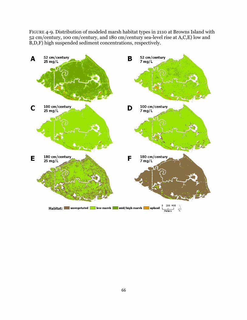
66  

FIGURE 4-9. Distribution of modeled marsh habitat types in 2110 at Browns Island with 52 cm/century, 100 cm/century, and 180 cm/century sea-level rise at A,C,E) low and B,D,F) high suspended sediment concentrations, respectively.

 

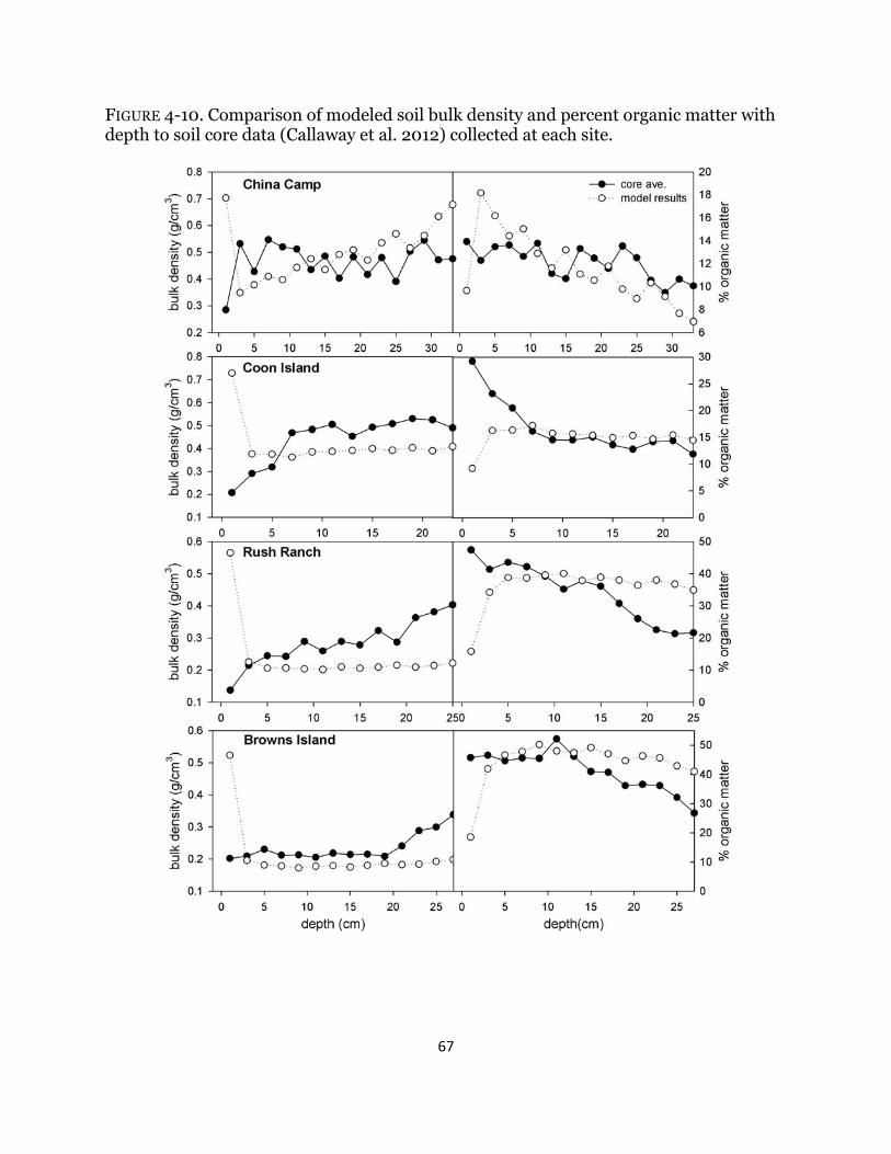
67  

FIGURE 4-10. Comparison of modeled soil bulk density and percent organic matter with depth to soil core data (Callaway et al. 2012) collected at each site.

 

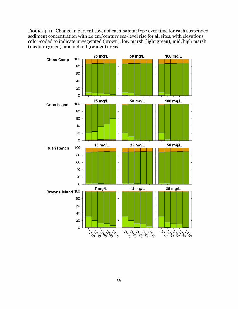
68  

FIGURE 4-11. Change in percent cover of each habitat type over time for each suspended sediment concentration with 24 cm/century sea-level rise for all sites, with elevations color-coded to indicate unvegetated (brown), low marsh (light green), mid/high marsh (medium green), and upland (orange) areas.

 

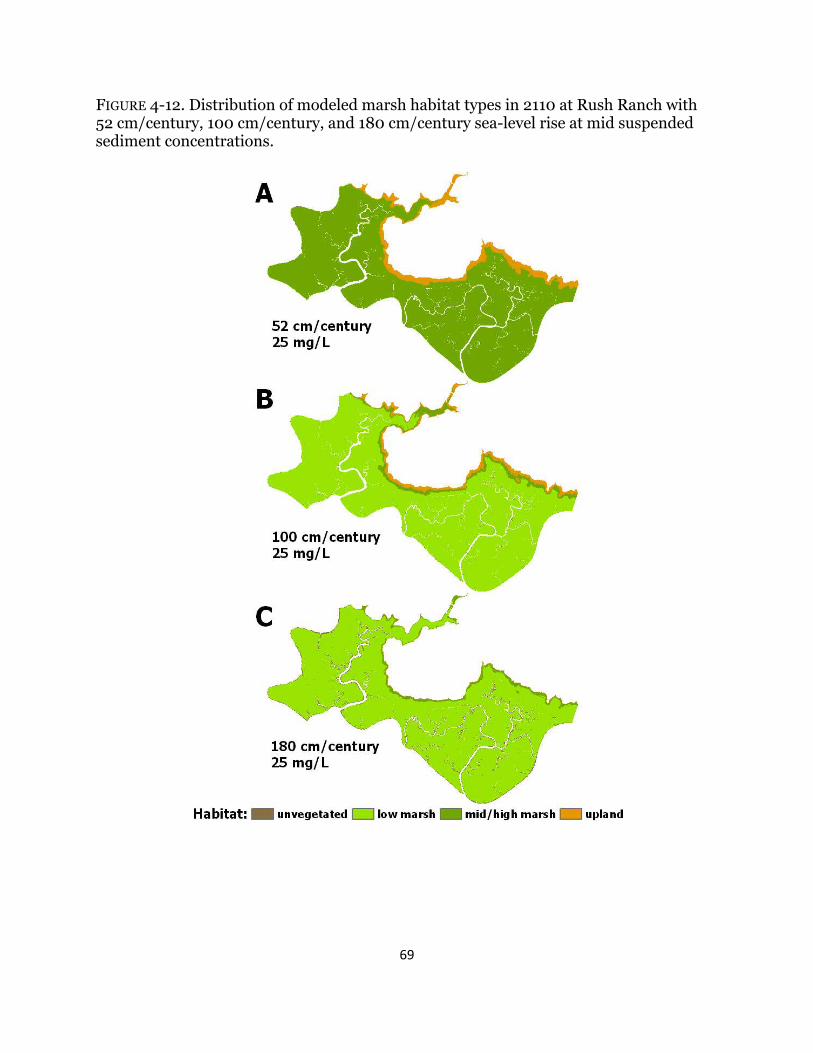
69  

FIGURE 4-12. Distribution of modeled marsh habitat types in 2110 at Rush Ranch with 52 cm/century, 100 cm/century, and 180 cm/century sea-level rise at mid suspended sediment concentrations.

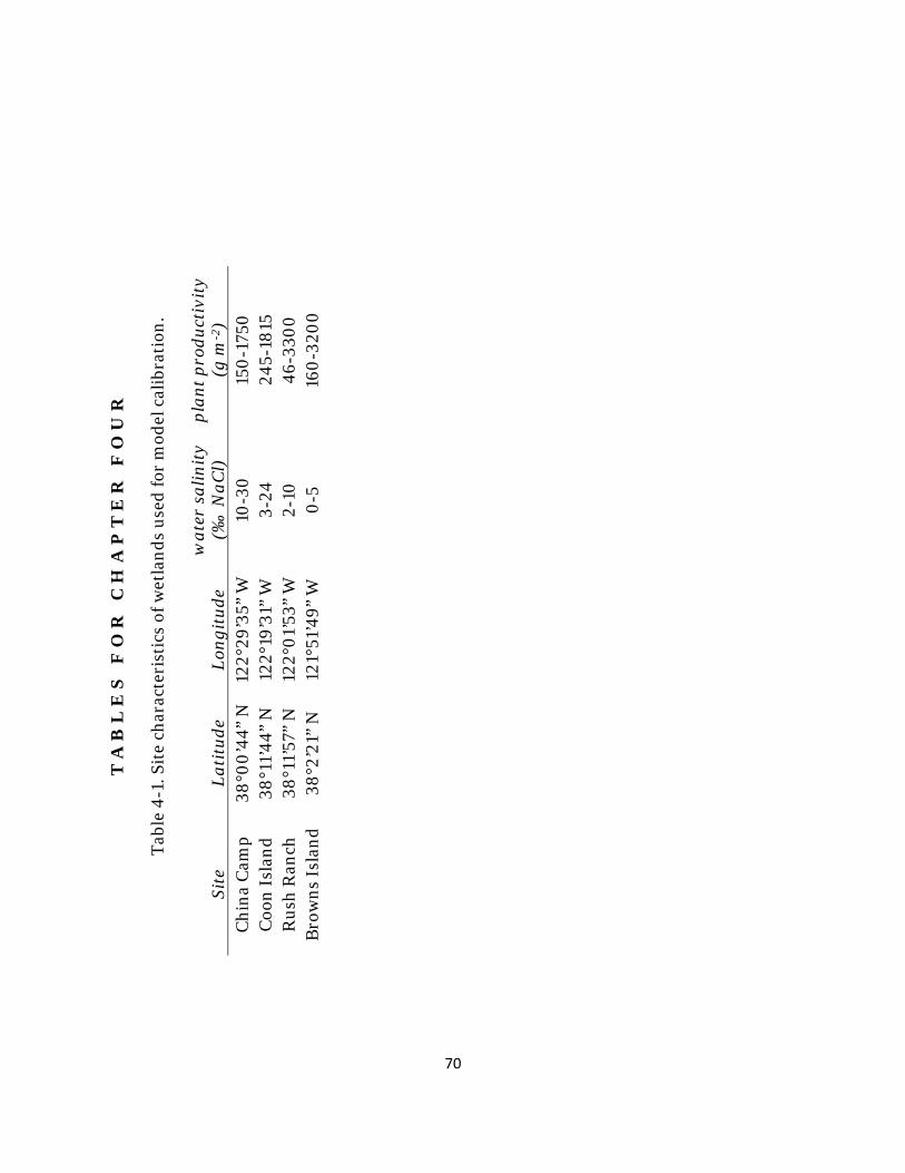
       70

T A

B L

E S

F

O R

C

H A

P T

E R

F

O U

R

Tab

le 4

-1. S

ite

char

acte

rist

ics

of w

etla

nd

s u

sed

for

mod

el c

alib

rati

on.

Site

L

ati

tud

e L

ong

itu

de

wa

ter

sali

nit

y (‰

Na

Cl)

p

lan

t p

rod

uct

ivit

y

(g m

-2)

Ch

ina

Cam

p

38°0

0’4

4”

N

122°

29’3

5” W

10

-30

15

0-1

750

C

oon

Isl

and

38

°11’

44

” N

12

2°19

’31”

W

3-24

24

5-18

15

Ru

sh R

anch

38

°11’

57”

N

122°

01’

53”

W

2-10

4

6-3

300

B

row

ns

Isla

nd

38

°2’2

1” N

12

1°51

’49

” W

0

-5

160

-320

0

 

 

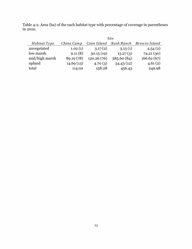
71  

Table 4-2. Area (ha) of the each habitat type with percentage of coverage in parentheses in 2010.

Site

Habitat Type China Camp Coon Island Rush Ranch Browns Island unvegetated 1.02 (1) 3.17 (2) 3.13 (1) 4.54 (2) low marsh 9.11 (8) 30.15 (19) 13.27 (3) 74.21 (30) mid/high marsh 89.19 (78) 120.26 (76) 385.60 (84) 166.62 (67) upland 14.69 (13) 4.70 (3) 54.43 (12) 4.61 (2) total 114.02 158.28 456.43 249.98

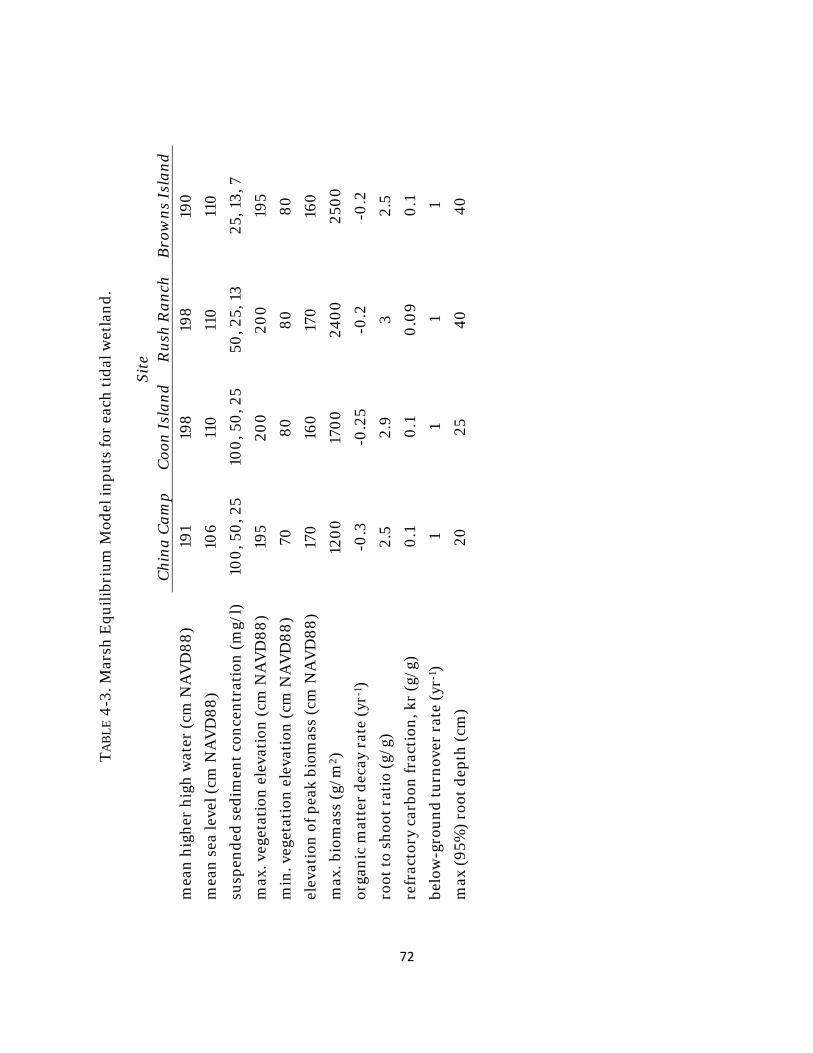
  72

TA

BL

E 4

-3. M

arsh

Equ

ilib

riu

m M

odel

inp

uts

for

eac

h t

idal

wet

lan

d.

 

Site

C

hin

a C

am

p

Coo

n I

sla

nd

R

ush

Ra

nch

B

row

ns

Isla

nd

m

ean

hig

her

hig

h w

ater

(cm

NA

VD

88

) 19

1 19

8

198

19

0

mea

n s

ea le

vel (

cm N

AV

D8

8)

106

11

0

110

11

0

susp

end

ed s

edim

ent

con

cen

trat

ion

(m

g/l)

10

0, 5

0, 2

5 10

0, 5

0, 2

5 50

, 25,

13

25, 1

3, 7

max

. veg

etat

ion

ele

vati

on (

cm N

AV

D8

8)

195

200

20

0

195

min

. veg

etat

ion

ele

vati

on (

cm N

AV

D8

8)

70

80

8

0

80

elev

atio

n o

f p

eak

biom

ass

(cm

NA

VD

88

) 17

0

160

17

0

160

max

. bio

mas

s (g

/m2 )

12

00

17

00

24

00

25

00

orga

nic

mat

ter

dec

ay r

ate

(yr-

1 )

-0.3

-0

.25

-0.2

-0

.2

root

to

shoo

t ra

tio

(g/g

) 2.

5 2.

9

3 2.

5

refr

acto

ry c

arbo

n f

ract

ion

, kr

(g/g

) 0

.1

0.1

0

.09

0

.1

belo

w-g

rou

nd

tu

rnov

er r

ate

(yr-

1 )

1 1

1 1

max

(9

5%)

root

dep

th (

cm)

20

25

40

4

0

 

73  

TABLE 4-4. Relative elevation key for determining cut-offs between habitat types.

Site China Camp Coon Island Rush Ranch Browns Island

unvegetated < -0.3 < -0.3 < -0.3 < -0.3 low marsh -0.3 - 0.7 -0.3 - 0.65 -0.3 - 0.74 -0.3 - 0.75 mid/high marsh 0.7 - 1.049 0.65 - 1.01 0.74 - 1.03 0.75 - 1.06 upland > 1.049 > 1.01 > 1.03 > 1.06

 

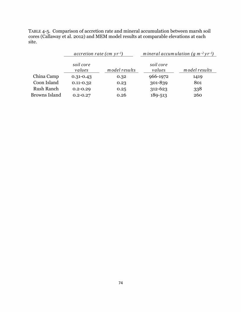
74  

TABLE 4-5. Comparison of accretion rate and mineral accumulation between marsh soil cores (Callaway et al. 2012) and MEM model results at comparable elevations at each site.

accretion rate (cm yr-1) mineral accumulation (g m-2 yr-1)

soil core values model results

soil core values model results

China Camp 0.31-0.43 0.32 966-1972 1419 Coon Island 0.11-0.32 0.23 301-839 801 Rush Ranch 0.2-0.29 0.25 312-623 338

Browns Island 0.2-0.27 0.26 189-513 260

 

75  

C H A P T E R F I V E

Conclusions and directions for future research

Tidal wetland ecosystems are dynamic coastal habitats that, in California, often occur at the complex nexus of aquatic environments, altered baylands, and modified upland habitat. Because of their prime coastal location and rich peat soil, many wetlands have been reduced, degraded, and/or destroyed, and yet their importance in carbon sequestration, nutrient and sediment filtering, flood dampening, and as habitat requires us to examine their maintenance and persistence in light of predicted climate change. My dissertation research focused on possibilities for wetland resilience in a changing climate in the San Francisco Bay Estuary across scales and using a suite of methodologies. I used several approaches – field experimentation, remote sensing, and modeling – to examine ways in which wetland plants might respond to accelerated sea-level rise, but also to understand how to measure and monitor their response across scales to a changing climate. Below, I highlight key findings from my research and discuss areas of future research and refinement.

Summary of Key Findings 1. Wetland plants have a high tolerance for increases in inundation. In Chapter Two, I examined wetland plant tolerances to increased inundation at depths comparable to projected century-end sea-level rise rates. While there are limits to growth and survival of any plant under increased inundation, results from this field experiment suggest that over the short term, wetland plant species can tolerate inundation rates greater than what they currently experience. Despite differences in tolerance, both of the widespread sedge species that I examined grew at water depths up to 60 cm deeper than they currently experience, even when water salinity levels were slightly increased. These results highlight that currently established populations of these species can likely persist with increased inundation rates in the face of accelerated rising sea levels, potentially increasing wetland resiliency over time. Both above and below-ground productivity will decrease as inundation levels increase, yet their ability to grow in spite of this is promising for short-term resistance to change. 2. Community interactions need to be incorporated into plant responses to increased sea-level rise. Examining plant community responses in a changing climate with no historic analogue presents challenges in understanding the direction and magnitude of species’ responses to climate change. Currently, both facilitation and competition can occur among species, typically, under both stressful and benign conditions, respectively. Through my field experiment investigating plant responses to increased inundation rates associated with predicted sea-level rise (detailed in Chapter Two), I discovered that a species more tolerant of increased inundation was also a better competitor as inundation and salinity stress increased. This finding was not predicted by current ecological theory and would not have been documented through investigation of single species responses. This result highlights that plant interactions currently seen in tidal wetlands are likely to

 

76  

change as stresses increase, and stress tolerance may directly affect the overall outcome of competitive interactions. 3. Litter cannot be ignored when estimating plant production using remotely sensed data. Many large-scale carbon assessment projects in wetlands are underway and there is a growing need to quantify plant production on large spatial scales for both carbon monitoring and incorporation into climate change modeling. Applying remote sensing methods used in forestry and agricultural systems for assessing primary production, I measured the fraction of photosynthetically active radiation, a key parameter for modeling gross primary productivity, at different heights within a very dense litter layer in a managed freshwater marsh and related values to spectral indices derived from in-situ field spectrometer data (Chapter Three). While I documented correlations between specific spectral indices and field data, a significant relationship only occurred when field measurements were taken above the litter layer, not at the ground surface where measurements normally occur. These methods calibrated from field measurements show promise, but are not yet reliable enough for widespread use. Better accounting of litter effects need to occur before wide-scale remotely sensed carbon measurements can be reliable in tidal wetlands. 4. Models of wetland resiliency require mechanistic modeling of both organic matter and mineral contribution to accretion. A broad suite of modeling efforts have occurred to investigate wetland resiliency with predicted increases in sea-level rise, and the majority of studies that apply results from the detailed one-dimensional models to at a wetland or estuary-wide scale do not incorporate the ecogeomorphic feedbacks affecting mineral and organic matter accretion with elevation. In Chapter Four, I used a rich dataset of plant productivity and physical processes in concert with an elevation-based soil cohort model that mechanistically models the individual effects and interactions of mineral input and organic matter on accretion. My results highlighted that inclusion of this interaction in examining predicted accelerated sea-level rise effects on marsh elevations gave a less pessimistic outcome than did models that use only model dynamics of mineral input. 5. Adjacent upland habitat is key for wetland resiliency. By applying projections of wetland elevation change with predicted sea-level rise at four tidal wetland sites, I found that wetlands with available adjacent upland habitat maintained vegetated elevations that could support mid and high marsh bird and mammal species. Under the highest rate of sea-level rise, formerly upland habitat contained the only vegetated areas. However, as shown in Chapter One, fixed land use activities on diked former baylands surrounding most of the San Francisco Bay Estuary precludes opportunities for marsh migration. In other parts of the estuary there are places for wetlands to migrate. Emphasis should be placed on obtaining and preserving these upland habitats for future wetland migration. Tidal wetland resilience to predicted sea-level requires an understanding of both individual plant and community-level responses in addition their interactions with

 

77  

sediment supply and adjacent land uses. Through each of these chapters, my results suggest promise for the future wetland landscape of San Francisco Bay Estuary, as well as multiple challenges. Wetland plants have the morphological and physiological adaptations to allow them to persist in environments that are regularly inundated and often salty, which are, respectively, oxygen-poor and toxic for most plant species. While I did discover that wetland plants can tolerate increased inundation up to and at least 60 cm higher than current depths, there are limits to the magnitude of inundation both in plant production and survival, which my field experiment and accretion modeling support. Scaling measurements of plant production up to the site level and across landscapes requires the integration of field measurements with remotely sensed measurements. In my investigation to test remotely sensed methods of measuring carbon stock, I was challenged in finding a reliable way of monitoring plant production remotely and currently measures of carbon storage will have to rely on intensive field work. More work will need to be conducted in this arena. Finally, while I was able to successfully calibrate a mechanistic model for wetland accretion across four wetlands in the San Francisco Bay Estuary, it is clear that the wetland landscape in the bay is threatened with rising sea levels, and there are a limited number of wetlands that will be able to migrate to higher ground as sea levels rise. Despite these challenges, my dissertation presents a robust and new understanding of how tidal wetlands might respond to predicted climate change. Directions for future research While my dissertation research begins to address tidal wetland resiliency in the face of sea-level rise, there are key aspects that could be expanded on for future research. My work examining the potential benefits of surrounding land use types on tidal wetlands could be improved by incorporating an elevation dataset into the model to highlight upland regions. This could further elucidate potential areas for wetland migration. Second, the field experiment investigating plant responses to increased rates of sea-level rise discussed in Chapter Two should be expanded to investigate more species common throughout the Estuary, examine how productivity changes when plants are grown alone and together, and incorporate more sites that have broader differences in salinity. Third, a network of plots needs to be established for regular measurement of suspended sediment concentrations within and across tidal wetlands. There is a dearth of data available from Pacific coast marshes. This is a key data gap yet one of the most critical of inputs into wetland accretion modeling. Models for widespread data collection across a suite of wetlands has occurred along the coast of the Gulf of Mexico (Coastwide Reference Monitoring System) and could similarly be applied in the San Francisco Bay Estuary. Fourth, incorporating lessons learned from the field experiment and review of modeling literature and data needs, another field experiment could be conducted to examine differences in accretion rates at each elevation within the experimental planters. A concurrent greenhouse experiment conducted under similar inundation regimes could

 

78  

be incorporated to isolate the plant’s role in accretion in the absence of suspended sediment. Fifth, efforts into developing a spatially explicit version of the mechanistic model used in Chapter 4 would significantly increase its ability to more accurately replicate marsh dynamics. Currently, individual points within a marsh do not interact as they would in a hydrodynamic model. With this improvement, however, the level of model complexity and processing time increases and its accessibility to wetland managers and practitioners might decrease. In the interim, a simple, point-based approach could be improved by adjusting sediment concentrations with channel distance, based on field measurements This dissertation addresses a number of key questions regarding wetland plant response to SLR, comments on available methods for scaling carbon estimates in wetland systems, and refines past models of wetland resilience by better use of ecogeomorphic feedbacks. As such it represents a step forward in understanding the potential resilience of the wetland landscape of the San Francisco Bay Estuary in a changing climate.

 

79  

R E F E R E N C E S

Adler, P. B., H. J. Dalgleish, and S. P. Ellner. 2012. Forecasting plant community impacts of climate variability and change: when do competitive interactions matter? Journal of Ecology 100:478-487.

Asner, G. P., C. A. Wessman, and S. Archer. 1998. Scale dependence of absorption of photosynthetically active radiation in terrestrial ecosystems. Ecological Applications 8:1003-1021.

Baldwin, A. and I. A. Mendelssohn. 1998. Effects of salinity and water level on coastal marshes: an experimental test of disturbance as a catalyst for vegetation change. Aquatic Botany 61:255-268.

Baumann, R. H., J. W. Day, Jr., and C. A. Miller. 1984. Mississippi deltaic wetland survival: Sedimentation versus coastal submergence. Science 224:1093-1095.

Bay Area Open Space Council. 2011. The Conservation Lands Network: San Francisco Bay area upland habitat goals project report. Berkeley, CA.

Bertness, M. D. and R. Callaway. 1994. Positive interactions in communities. TRENDS in Ecology and Evolution 9:191-193.

Boesch, D. F., M. N. Josselyn, A. J. Mehta, J. T. Morris, W. K. Nuttle, C. A. Simenstad, and D. J. P. Swift. 1994. Scientific assessment of coastal wetland loss, restoration and management in Louisiana. Journal of Coastal Research 20:1-103.

Bridgham, S. D., J. P. Megonigal, J. K. Keller, N. B. Bliss, and C. Trettin. 2006. The carbon balance of North American wetlands. Wetlands 26:889-916.

Bromberg Gedan, K., B. R. Silliman, and M. D. Bertness. 2009. Centuries of human-driven change in salt marsh ecosystems. Annual Review of Marine Science 1:117-141.

Brooker, R. W. 1996. Plant-plant interactions and environmental change. New Phytologist 171:271-284.

Broome, S. W., I. A. Mendelssohn, and K. L. McKee. 1995. Relative growth of Spartina patens (Ait.) Muhl. and Scirpus olneyi Gray occurring in a mixed stand as affected by salinity and flodding depth. Wetlands 15:20-30.

Byrd, K. B., N. M. Kelly, and E. Van Dyke. 2004. Decadal changes in a Pacific estuary: a multi-source remote sensing approach for historical ecology. GIScience and Remote Sensing 41:347-370.

 

80  

Cahoon, D. R., P. Hensel, J. Rybczyk, K. L. McKee, C. E. Proffitt, and B. C. Perez. 2003. Mass tree mortality leads to mangrove peat collapse at Bay Islands, Honduras after Hurrican Mitch. Journal of Ecology 91:1093-1105.

Cahoon, D. R., P. F. Hensel, T. Spencer, D. J. Reed, K. L. McKee, and N. Saintilan. 2006. Coastal wetland vulnerability to relative sea-level rise: wetland elevation trends and process controls. Pages 271-292 in J. T. A. Verhoeven, D. Beltman, R. Bobbink, and D. F. Whigham, editors. Wetlands and Natural Resource Management: Ecological Studies. Springer, Berlin.

Callaway, J. C., E. L. Borgnis, R. E. Turner, and C. S. Milan. 2012. Carbon sequestration and sediment accretion in San Francisco Bay tidal wetlands. Estuaries and Coasts 35:1163-1181.

Callaway, J. C., J. A. Nyman, and R. D. DeLaune. 1996. Sediment accretion in coastal wetlands: A review and a simulation model of processes. Current Topics in Wetland Biogeochemistry 2:2-23.

Callaway, J. C., V. T. Parker, M. C. Vasey, and L. M. Schile. 2007. Emerging issues for the restoration of tidal marsh ecosystems in the context of predicted climate change. Madrono 54:234-248.

Cayan, D. R., E. P. Maurer, M. D. Dettinger, M. Tyree, and K. Hayhoe. 2008. Climate change scenarios for the California region. Climatic Change 87:21-42.

Chen, Z. Y., J. F. Li, H. T. Shen, and Z. H. Wang. 2001. Yangtze River of China: historical analysis of discharge variability and sediment flux. Geomorphology 41:77-91.

Cherry, J. A., K. L. McKee, and J. B. Grace. 2009. Elevated CO2 enhances biological contributions to elevation change in coastal wetlands by offsetting stressors associated with sea-level rise. Journal of Ecology 97:67-77.

Chmura, G. L., S. C. Anisfeld, D. R. Cahoon, and J. C. Lynch. 2003. Global carbon sequestration in tidal, saline wetland soils. Global Biogeochemical Cycles 17:1111.

Cloern, J. E., N. Knowles, L. R. Brown, D. Cayan, M. D. Dettinger, T. L. Morgan, D. H. Schoellhamer, M. T. Stacey, M. van der Wegen, R. W. Wagner, and A. D. Jassby. 2011. Projected evolution of California's San Francisco Bay-Delta river system in a century of climate change. PloS ONE 6:e24465.

Cohen, A. N. and J. T. Carlton. 1998. Accelerating invasion rate in a highly invaded estuary. Science 279:555-558.

 

81  

Connell, J. H. 1961. The influence of interspecific competition and other factors on the distribution of the barnacle Chthamalus stellatus. Ecology 42:710-723.

Conomos, T. J. 1979. Properties and circulation of San Francisco Bay waters. In San Francisco Bay: the urbanized estuary. Pages 47-84 in T. J. Conomos, editor. San Francisco Bay: the Urbanized Estuary. Pacific Division of the American Association for the Advancement of Science, San Francisco.

Cook, B. D., P. V. Bolstad, E. Næsset, R. S. Anderson, S. Garrigues, J. T. Morisette, J. Nickeson, and K. J. Davis. 2009. Using LiDAR and QuickBird data to model plant production and quantify uncertainties associated with wetland detection and land cover generalizations. Remote Sensing of Environment 113:2366-2379.

Craft, C., J. Clough, J. Ehman, S. Joye, R. Park, S. Pennings, H. Guo, and M. Machmuller. 2008. Forecasting the effects of accelerated sea-level rise on tidal marsh ecosystem services. Frontiers in Ecology and the Environment 7:73-78.

Craft, C., J. Clough, J. Ehman, S. Joye, R. Park, S. Pennings, H. Y. Guo, and M. Machmuller. 2009. Forecasting the effects of accelerated sea-level rise on tidal marsh ecosystem services. Frontiers in Ecology and the Environment 7:73-78.

Crain, C. M., B. R. Silliman, S. L. Bertness, and M. D. Bertness. 2004. Physical and biotic drivers of plant distribution across estuarine salinity gradients. Ecology 85:2539-2549.

Crooks, S., S. Emmett-Mattox, and J. Findsen. 2010. Findings of the National Blue Ribbon Panel on the development of a greenhouse gas offset protocol for tidal wetlands restoration and management: Action plan to guide protocol development. Page 15 pp. Restore America's Estuaries, Philip Williams & Associates, Ltd., and Science Applications International Corporation.

Daubenmire, R. F. 1959. Canopy coverage method of vegetation analysis. Northwest Science 33:43-64.

Day, J. W., Jr., D. Pont, P. F. Hensel, and C. Ibañez. 1995. Impacts of sea-level rise on deltas in the Gulf of Mexico and the Mediterranean: The importance of pusling events to sustainability. Estuaries 18:636-647.

Department of Commerce, National Oceanic and Atmospheric Administration, National Ocean Service, and Coastal Services Center. 2012. 2009-2011 California Coastal Conservancy Coastal LiDAR Project. NOAA's Ocean Service Coastal Services Center, Charleston, SC.

 

82  

Dettinger, M. D. 2005. From climate change spaghetti to climate-change distributions for 21st century California. San Francisco Estuary and Watershed Science 3.

Deverel, S. J. and D. A. Leighton. 2010. Historic, recent, and future subsidence, Sacramento-San Joaquin Delta, California, USA. San Francisco Estuary and Watershed Science 8:23 pp.

Deverel, S. J. and S. Rojstaczer. 1996. Subsidence of agricultural lands in the Sacramento San Joaquin Delta, California: Role of aqueous and gaseous carbon fluxes. Water Resources Research 32:2359-2367.

Di Bella, C. M., J. M. Paruelo, J. E. Becerra, C. Bacour, and F. Baret. 2004. Effect of senescent leaves on NDVI-based estimates of fAPAR: experimental and modelling evidences. International Journal of Remote Sensing 25:5415-5427.

Donnelly, J. P. and M. D. Bertness. 2001. Rapid shoreward encroachment of salt marsh cordgrass in response to accelerated sea-level rise. Proceedings of the National Academy of Science 98:14218-14223.

Drexler, J. Z., C. S. de Fontaine, and T. A. Brown. 2009. Peat accretion histories during the past 6,000 years in marshes of the Sacramento-San Joaquin Delta of California, USA. Estuaries and Coasts 32:871-892.

Drexler, J. Z., C. S. d. Fontaine, and D. L. Knifong. 2007. Age Determination of the Remaining Peat in the Sacramento–San Joaquin Delta, California, USA USGS.

Elsey-Quirk, T., D. M. Seliskar, C. K. Sommerfield, and J. L. Gallagher. 2011. Salt marsh carbon pool distribution in a mid-Atlantic lagoon, USA: sea level rise implications. Wetlands 31.

Emmett-Mattox, S., S. Crooks, and J. Findsen. 2011. Grasses and gases. The Environmental Forum 28:30-35.

Enright, C. and S. D. Culberson. 2009. Salinity trends, variability, and control in the northern reach of the San Francisco Estuary. San Francisco Estuary & Watershed Science 7:1-28.

Erickson, J. E., J. P. Megonigal, G. Peresta, and B. G. Drake. 2007. Salinity and sea-level mediate elevated CO2 effects on C3-C4 plant interactions and tissue nitrogen in a Chesapeake Bay tidal wetland. Global Change Biology 13:202-215.

ESRI Inc. 2010. Environmental Science Research Institute.

 

83  

Fagherazzi, S., M. L. Kirwan, S. M. Mudd, G. G. Guntenspergen, S. Temmerman, A. D'Alpaos, J. van den Koppel, J. Rybczyk, E. Reyes, C. Craft, and J. Clough. 2012. Numerical models of salt marsh evolution: ecological, geomorphic, and climatic factors. Reviews of Geophysics 50:RG1002.

Foxgrover, A. C., S. A. Higgins, M. K. Ingraca, B. E. Jaffe, and R. E. Smith. 2004. Deposition, erosion, and bathymetric change in South San Francisco Bay: 1858-1983. U.S. Geological Survey Open-File Report.

Fretwell, J. D., J. S. Williams, and P. J. Redman, editors. 1996. National Water Summary on Wetland Resources, Washington, DC.

Gilman, S. E., M. C. Urban, J. J. Tewksbury, G. W. Gilchrist, and R. D. Holt. 2010. A framework for community interactions under climate change. Trends in Ecology & Evolution 25:325-331.

Gitelson, A. A. 2012. Remote sensing estimation of crop biophysical characteristics at various scales. Pages 329-360 in P. S. Thenkabail, J. G. Lyon, and A. Huete, editors. Hyperspectral remote sensing of vegetation. CRC Press, Boca Raton.

Gitelson, A. A., Y. Peng, J. G. Masek, D. C. Rundquist, S. Verma, A. Suyker, J. M. Baker, J. L. Hatfield, and T. Meyers. 2012. Remote estimation of crop gross primary production with Landsat data. Remote Sensing Of Environment 121:404-414.

Gleick, P. H. 1987a. The development and testing of a water-balance model for climate impact assessment: Modeling the Sacramento Basin. Water Resources Research 23:1049-1061.

Gleick, P. H. 1987b. Regional hydrologic consequences of increases in atmospheric carbon dioxide and other trace gases. Climatic Change 10:137-161.

Gleick, P. H. and E. L. Chalecki. 1999. The impacts of climatic changes for water resources of he Colorado and Sacramento-San Joaquin river basins. Journal of the American Water Resources Association 35:1429-1441.

Goals Project. 1999. Baylands ecosystem habitat goals: A report of habitat recommendations prepared by the San Francisco Bay Area Wetlands Ecosystem Goals Project. U.S. Environmental Protection Agency, San Francisco, CA.

Goman, M. and L. Wells. 2000. Trends in the river flow affecting the northeastern reach of the San Francisco Bay Estuary over the past 7000 years. Quarternary Research 54:206-217.

 

84  

Greiner La Peyre, M. K., J. B. Grace, E. Hahn, and I. A. Mendelssohn. 2001. The importance of competition in regulation plant species abundance along a salinity gradient. Ecology 82:62-69.

Grewell, B. J., J. C. Callaway, and W. R. Ferren. 2007. Estuarine wetlands. Pages 124-154 in M. G. Barbour, T. Keeler-Wolf, and A. A. Schoenherr, editors. Terrestrial Vegetation of California, 3rd edition. University of California Press, Berkeley.

Grinsted, A., J. C. Moore, and S. Jevrejeva. 2010. Reconstructing sea level from paleo and projected temperatures 200 to 2100 AD. Climate Dynamics 34:461–472.

Guo, H. and S. C. Pennings. 2012. Mechanisms mediating plant distributions across estuarine landscapes in a low-latitude tidal estuary. Ecology 93:90-100.

Guo, X. and B. C. Si. 2008. Characterizing LAI spatial and temporal variability using a wavelet approach. Pages 31-34 in XXIst International Society for Photogrammetry and Remote Sensing Congress, Technical Commission VII. ISPRS, Beijing.

Hacker, S. D. and M. D. Bertness. 1999. Experimental evidence for factors maintaining plant species diversity in a New England salt marsh. Ecology 80:2064-2073.

Halpern, B. S., B. R. Silliman, J. D. Olden, J. P. Bruno, and M. D. Bertness. 2007. Incorporating positive interactions in aquatic restoration and conservation. Frontiers in Ecology and the Environment 5:153-160.

Hillyer, R. and M. R. Silman. 2010. Changes in species interactions across a 2.5 km elevation gradient: effects on plant migration in repsonse to climate change. Global Change Biology 16:3205-3214.

Hladik, C. and M. Alber. 2012. Accuracy assessment and correction of a LIDAR-derived salt marsh digital elevation model. Remote Sensing Of Environment 121:224-235.

Howard, R. J. and I. A. Mendelssohn. 2000. Structure and composition of oligohaline marsh plant communities exposed to salinity pulses. Aquatic Botany 68:143-164.

Ibàñez, C., N. Prat, and A. Canicio. 1996. Changes in the hydrology and sediment transport produced by large dams on the lower Ebro river and its estuary. Regulated Rivers: Research and Management 12:51-62.

Ikegami, M., D. F. Whigam, and M. J. A. Werger. 2007. Responses of rhizome length and ramet production to resource availability in the clonal sedge Scirpus olneyi A. Gray. Plant Ecology 189:247-259.

 

85  

Inoue, Y., J. Penuelas, A. Miyata, and M. Mano. 2008. Normalized difference spectral indices for estimating photosynthetic efficiency and capacity at a canopy scale derived from hyperspectral and CO2 flux measurements in rice. Remote Sensing of Environment 112:156-172.

Intergovernmental Panel on Climate Change. 2007. Summary for Policymakers. Cambridge University Press, Cambridge, UK and New York, USA.

Josselyn, M. 1983. The ecology of San Francisco Bay tidal marshes: a community profile. FWS 10BS-82/23, U.S. Fish and Wildlife Service, Division of Biological Services, Washington, D.C.

Jump, A. S. and J. Peñuelas. 2005. Running to stand still: adaptation and the response of plants to rapid climate change. Ecology Letters 8:1010-1020.

Kearney, M. S. and J. C. Stevenson. 1991. Island land loss and marsh vertical accretion rate evidence for historical sea-level changes in Chesapeake Bay. Journal of Coastal Research 7:403-415.

Kearney, M. S., D. Stutzer, K. Turpie, and J. C. Stevenson. 2009. The effects of tidal inundation on the reflectance characteristics of coastal marsh vegetation. Journal of Coastal Research 25:1177-1186.

Kimmerer, W. 2002. Physical, biological, and management responses to variable freshwater flow into the San Francisco Estuary. Estuaries and Coasts 25:1275-1290.

Kirwan, M. L., G. G. Guntenspergen, and J. T. Morris. 2009. Latitudinal trends in Spartina alterniflora productivity and the response of coastal marshes to global change. Global Change Biology 15:1982-1989.

Kirwan, M. L. and G. R. Guntenspergen. 2012. Feedbacks between inundation, root production, and shoot growth in a rapidly submerging brackish marsh. Journal of Ecology 100:764-770.

Kirwan, M. L., G. R. Guntenspergen, A. D'Alpaos, and J. T. Morris. 2010a. Limits on the adaptability of coastal marshes to rising sea level. Geophysical Research Letters 37:L23401.

Kirwan, M. L., G. R. Guntenspergen, A. D'Alpaos, J. T. Morris, S. M. Mudd, and S. Temmerman. 2010b. Limits on the adaptability of coastal marshes to rising sea level. Geophysical Research Letters 37:L23401.

 

86  

Kirwan, M. L. and S. M. Mudd. 2012. Response of salt-marsh carbon accumulation to climate change. Nature 489:550-554.

Kirwan, M. L. and A. B. Murray. 2007. A coupled geomorphic and ecological model of tidal marsh evolution. Proceedings of the National Academy of Science 104:6118-6122.

Klemas, V. 2011. Remote sensing of wetlands: case studies comparing practical techniques. Journal of Coastal Research 27:418-427.

Knowles, N. and D. R. Cayan. 2002. Potential effects of global warming on the Sacramento/San Joaquin watershed and the San Francisco estuary. Geophysical Research Letters 29:1-5.

Knowles, N. and D. R. Cayan. 2004. Elevational dependence of projected hydrologic changes in the San Francisco Estuary and watershed. Climatic Change 62:319-336.

Knowles, N., M. D. Dettinger, and D. R. Cayan. 2006. Trends in snowfall versus rainfall in the Western United States. Journal of Climate 19:4545-4559.

Konisky, R. A. and D. M. Burdick. 2004. Effects of stressors on invasive and halophytic plants of New England salt marshes: a framework for predicting response to tidal restoration. Wetlands 24:434-447.

Krone, R. B. 1987. A method for simulating historic marsh elevations. Pages 316-323 in N. C. Krause, editor. Coastal Sediments '87. American Society of Civil Engineers, New York, NY.

Langley, J. A., K. L. McKee, D. R. Cahoon, J. A. Cherry, and J. P. Megonigal. 2009. Elevated CO2 stimulates marsh elevation gain, counterbalancing sea-level rise. Proceedings of the National Academy of Sciences 106:6182-6186.

Leck, M. A., V. T. Parker, L. M. Schile, and D. F. Whigam. 2009. Plant communities of tidal freshwater wetlands of the continental USA and southeaster Canada. Pages 41-58 in A. Barendregt, D. F. Whigam, and A. Baldwin, editors. Tidal Freshwater Wetlands. Backhys Publishers, Leiden.

Lessmann, J. M., I. A. Mendelssohn, M. W. Hester, and K. L. McKee. 1997. Population variation in growth response to flooding in three marsh species. Ecological Engineering 8:31-47.

 

87  

Lettenmaier, D. P. and T. Y. Gan. 1990. Hydrologic sensitivities of the Sacramento-San Joaquin River basin, California, to global warming. Water Resources Research 26:69-86.

Luo, W., Y. Xie, X. Che, F. Li, and X. Qin. 2010. Competition and facilitation in three marsh plants in response to a water-level gradient. Wetlands 30:525-530.

Maestre, F. T., M. A. Bowker, C. Escolar, M. D. Puche, S. Soliveres, S. Maltez-Mouro, P. García-Palacios, A. P. Castillo-Monroy, I. Martínez, and A. Escudero. 2010. Do biotic interactions modulate ecosystem functioning along stress gradients? Insights from semi-arid plant and biological soil-crust communities. Philosophical Transactions of the Royal Society of London, Series B 365:2057-2070.

Maestre, F. T., R. M. Callaway, F. Valladares, and C. J. Lortie. 2009. Refining the stress-gradient hypothesis for competition and facilitation in plant communities. Journal of Ecology 97:199-205.

Marion, C., E. J. Anthony, and A. Trentesaux. 2009. Short-term (<=2 yrs) estuarine mudflat and saltmarsh sedimentation: high-resolution data from ultrasonic altimetery, rod surface-elevation table, and filter traps. Estuarine, Coastal and Shelf Science 83:475-484.

Maselli, F., D. Papale, N. Puletti, G. Chirici, and P. Corona. 2009. Combining remote sensing and ancillary data to monitor the gross productivity of water-limited forest ecosystems. Remote Sensing of Environment 113:657-667.

McKee, K. L., D. R. Cahoon, and I. C. Feller. 2007. Caribbean mangroves adjust to rising sea level through biotic controls on change in soil elevation. Global Ecology and Biogeography 16:545-556.

McKee, K. L. and I. A. Mendelssohn. 1989. Response of a fresh-water marsh plant community to increased salinity and increased water level. Estuarine and Coastal Marine Science 11:27-40.

Middleton, E. M., K. F. Huemmrich, Y. Cheng, and H. A. Margolis. 2012. Spectral bioindicators of photosynthetic efficiency and vegetation stress. Pages 265-288 in P. S. Thenkabail, J. G. Lyon, and A. Huete, editors. Hyperspectral remote sensing of vegetation. CRC Press, Boca Raton.

Miller, R. L., M. S. Fram, R. Fujii, and G. Wheeler. 2008. Subsidence reversal in a re-established wetland in the Sacramento-San Joaquin Delta, California, USA. San Francisco Estuary and Watershed Science.

 

88  

Miller, R. L. and R. Fujii. 2010. Plant community, primary productivity, and environmental conditions following wetland re-establishment in the Sacramento-San Joaquin Delta, California. Wetland Ecology and Management 18:1-16.

Monismith, S. G., W. Kimmerer, J. R. Burau, and M. T. Stacey. 2002. Structure and flow-induced variability of the subtidal salinity field in northern San Francisco Bay. Journal of Physical Oceanography 32:3003-3019.

Morris, J. T. 2007. Estimating net primary production of salt marsh macrophytes. Oxford University Press, New York, NY.

Morris, J. T. and W. B. Bowden. 1986. A mechanistic, numerical model of sedimentation, mineralization and decomposition for marsh sediments. Soil Science Society of America Journal 50:96-105.

Morris, J. T., J. Edwards, S. Crooks, and E. Reyes. 2012. Assessment of carbon sequestration potential in coastal wetlands. Pages 517-531 in R. Lal, K. Lorenz, R. Huttl, B. U. Schneider, and J. von Braun, editors. Recarbonization of the biosphere: ecosystems and the global carbon cycle. Springer, New York.

Morris, J. T. and B. Haskin. 1990. A 5-yr record of aerial primary production and stand characteristics of Spartina alterniflora. Ecology 71:2209-2217.

Morris, J. T., P. V. Sundareshwar, C. T. Nietch, B. Kjerfve, and D. R. Cahoon. 2002. Responses of coastal wetlands to rising sea level. Ecology 83:2869-2877.

Mudd, S. M., A. D'Alpaos, and J. T. Morris. 2010. How does vegetation affect sedimentation on tidal marshes? Investigating particle capture and hydrodynamic controls on biologically mediated sedimentation. Journal of Geophysical Research 115:F03029.

Mudd, S. M., S. M. Howell, and J. T. Morris. 2009. Impact of dynamic feedbacks between sedimentation, sea-level rise, and biomass production on near-surface marsh stratigraphy and carbon accumulation. Estuarine, Coastal and Shelf Science 82:377-389.

National Research Council. 2012. Sea-level rise for the coasts of California, Oregon, and Washington: past, present, and future. The National Academies Press, Washington, D.C.

National Research Council. Committee on the Engineering Implications of Changes in Relative Mean Sea Level. 1987. Responding to changes in sea leve: engineering implications. National Academy Press, Washington D.C.

 

89  

Neubauer, S. C., I. C. Anderson, J. A. Constantine, and S. A. Kuehl. 2002. Sediment deposition and accretion in a mid-Atlantic (U.S.A.) tidal freshwater marsh. Estuarine, Coastal and Shelf Science 54:713-727.

Nichols, F. H., J. E. Cloern, S. N. Luoma, and D. H. Peterson. 1986. The modification of an estuary. Science 231:567-573.

Numata, I. 2012. Characterization on pastures using field and imaging spectrometers. Pages 207-226 in P. S. Thenkabail, J. G. Lyon, and A. Huete, editors. Hyperspectral remote sensing of vegetation. CRC Press, Boca Raton.

Nur, N., L. Salas, S. Veloz, J. Wood, L. Liu, and B. G. 2012. Assessing vulnerability of tidal marsh birds to climate change through the analysis of population dynamics and viability. Technical Report. Version 1.0. Report to the California Landscape Conservation Cooperative., PRBO Conservation Science, Petaluma.

Nyman, J. A., R. D. DeLaune, and W. H. Patrick. 1990. Wetland soil formation in the rapidly subsiding Mississippi river deltaic plain: mineral and organic matter relationships. Estuarine, Coastal and Shelf Science 31:57-69.

Nyman, J. A., R. D. DeLaune, H. H. Roberts, and W. H. Patrick, Jr. 1993. Relationship between vegetation and soil formation in a rapidly submerging coastal marsh. Marine Ecology Progress Series 96:269-278.

Nyman, J. A., R. J. Walters, R. D. Delaune, and W. H. Patrick. 2006. Marsh vertical accretion via vegetative growth. Estuarine, Coastal and Shelf Science 69:370-380.

Orr, M., S. Crooks, and P. B. Williams. 2003. Will restored tidal marshes be sustainable? San Francisco Estuary and Watershed Science 1:1-33.

Palaima, A., editor. 2012. Ecology, Conservation, and Restoration of Tidal Marshes: the San Francisco Estuary. University of California Press, Berkeley, CA.

Parker, V. T., J. C. Callaway, L. M. Schile, M. C. Vasey, and E. R. Herbert. 2012. Tidal vegetation: spatial and temporal dynamics. Pages 97-111 in A. Palaima, editor. Ecology, Conservation, and Restoration of Tidal Marshes: the San Francisco Estuary. University of California Press, Berkeley, CA.

Parker, V. T., E. R. Herbert, J. C. Callaway, L. M. Schile, and M. C. Vasey. 2011a. Impact of climate change on San Francisco Bay-Delta tidal wetlands. Pages 239-244 in J. W. Willoughby, B. K. Orr, K. A. Schierenbeck, and N. J. Jensen, editors. California Native Plant Society 2009 Conservation Conference Proceedings: Strategies and Solutions. California Native Plant Society, Sacramento, CA.

 

90  

Parker, V. T., L. M. Schile, M. C. Vasey, and J. C. Callaway. 2011b. Efficiency in assessment and monitoring methods: scaling down gradient-directed transects. Ecosphere 2:99.

Parmesan, C. and G. Yohe. 2003. A globally coherent fingerprint of climate change impacts across natural systems. Nature 421:37-42.

Pendleton, L., D. C. Donato, B. C. Murray, S. Crooks, W. A. Jenkins, S. Sifleet, C. Craft, J. W. Fourqurean, J. B. Kauffman, N. Marbà, P. Megonigal, E. Pidgeon, D. Herr, D. Gordon, and A. Baldera. 2012. Estimating global “Blue Carbon” emissions from conversion and degradation of vegetated coastal ecosystems. Page e43542 PLoS ONE. Public Library of Science.

Peng, Y. and A. A. Gitelson. 2012. Remote estimation of gross primary productivity in soybean and maize based on total crop chlorophyll content. Remote Sensing of Environment 117:440-448.

Pennings, S. C. and R. M. Callaway. 1992. Salt marsh plant zonation: the relative importance of competition and physical factors. Ecology 73:681-690.

Pennings, S. C., M. Grant, and M. D. Bertness. 2005. Plant zonation in low-latitude salt marshes: disentangling the roles of flooding, salinity, and competition. Journal of Ecology 93:159-167.

Penuelas, J., M. F. Garbulsky, and I. Filella. 2011. Photochemical reflectance index (PRI) and remote sensing of plant CO2 uptake. New Phytologist 191:596-599.

Phinn, S. R. 1998. A framework for selecting appropriate remotely sensed data dimensions for environmental monitoring and management. International Journal of Remote Sensing 19:3457-3463.

Rahmstorf, S. 2007. A semi-empirical approach to projecting future sea-level rise. Science 315:368-370.

Rasse, D. P., G. Peresta, and B. G. Drake. 2005. Seventeen years of elevated CO2 exposure in a Chesapeake Bay wetland: sustained by contrasting responses of plant growth and CO2 uptake. Global Change Biology 11:369-377.

Ravindranath, N. H. and M. Ostwald. 2007. Remote sensing and GIS techniques for terrestrial carbon inventory. Pages 181-199 in M. Beniston, editor. Carbon Inventory Methods: Handbook for Greenhouse Gas Inventory, Carbon Mitigation and Roundwood Production Projects. Springer, Netherlands.

 

91  

Reed, D. J. 1995. The response of coastal marshes to sea-level rise: Survival or submergence. Earth Surface Processes and Landforms 20:39-48.

Rocha, A. V. and M. L. Goulden. 2009. Why is marsh productivity so high? New insights from eddy covariance and biomass measurements in a Typha marsh. Agricultural and Forest Meteorology 149:159-168.

Rogers, K., N. Saintilan, and C. Copeland. 2012. Modelling wetland surface elevation dynamics and its application to forecasting the effect of sea-level rise on estuarine wetlands. Ecological Modelling 244:148-157.

Rybczyk, J. M. and J. C. Callaway. 2009. Surface elevation models. Pages 835-853 in G. M. E. Perillo, E. Wolanski, D. Cahoon, and M. M. Brinson, editors. Coastal Wetlands: an integrated ecosystem approach. Elsevier, Amsterdam, The Netherlands.

San Francisco Estuary Project. 1991. Status and trends report on wetlands and related habitats in the San Francisco Estuary : Public report. San Francisco Estuary Project, Oakland, Calif.

Sanderson, E. W., T. C. Foin, and S. L. Ustin. 2001. A simple empirical model of salt marsh plant spatial distributions with respect to a tidal channel network. Ecological Modelling 139:293-307.

SAS, I. 2009. SAS, version 9.2. SAS Institue Inc., Cary, North Carolina.

SAS Inc. 2009. SAS version 9.2. SAS Institute Inc., Cary.

Schile, L. M., J. C. Callaway, V. T. Parker, and M. C. Vasey. 2011. Salinity and inundation influence productivity of the halophytic plant Sarcocornia pacifica. Wetlands 31:1165-1174.

Schoellhamer, D. H. 2011. Sudden clearing of estuarine waters upon crossing the threshold from transport to supply regulation of sediment transport as an erodible sediment pool is depleted: San Francisco Bay, 1999. Estuaries and Coasts 34:885-899.

Seliskar, D. M. 1990. The role of waterlogging and sand accretion in modulating the morphology of the dune slack plant Scirpus americanus. Canadian Journal of Botany 68:1780-1787.

Stahle, D. W., M. D. Therrell, M. K. Cleaveland, D. Cayan, M. Dettinger, and N. Knowles. 2001. Ancient blue oaks reveal human impact on San Francisco Bay salinity. EOS 82:141-145.

 

92  

StataCorp LP. 1985-2009. Stata/IC 11.2. StataCorp LP, College Station.

Stevenson, J. C., L. G. Ward, and M. S. Kearney. 1986. Vertical accretion in marshes with varying rates of sea level rise. Pages 241-259 in D. A. Wolfe, editor. Estuarine variability. Academic Press, San Diego, CA.

Stralberg, D., M. Brennan, J. C. Callaway, J. K. Wood, L. M. Schile, D. Jongsomjit, M. Kelly, V. T. Parker, and S. Crooks. 2011. Evaluating tidal marsh sustainability in the face of sea-level rise: a hybrid modeling approach applied to San Francisco Bay. PloS ONE 6:e27388.

Suding, K. N., D. E. Goldberg, and K. M. Hartman. 2003. Relationships among species traits: separating levels of response and identifying linkages to abundance. Ecology 84:1-16.

Suttle, K. B., M. A. Thomsen, and M. E. Power. 2007. Species interactions reverse grassland response to changing climate. Science 315:640-642.

Syvitski, J. P. M., A. J. Kettner, I. Overeem, E. W. H. Hutton, M. T. Hannon, G. R. Brakenridge, J. Day, C. Vorosmarty, Y. Saito, L. Giosan, and R. J. Nicholls. 2009. Sinking deltas due to human activities. Nature Geoscience 2:681-686.

Syvitski, J. P. M., C. J. Vörösmarty, A. J. Kettner, and P. Green. 2005. Impact of humans on the flux of terrestrial sediment to the global coastal ocean. Science 308:376-380.

Thenkabail, P. S., E. A. Enclona, M. S. Ashton, and B. Van Der Meer. 2004. Accuracy assessments of hyperspectral waveband performance for vegetation analysis applications. Remote Sensing of Environment 91:354.

Thom, R. M. 1992. Accretion rates of low intertidal salt marshes in the Pacific Northwest. Wetlands 12:147-156.

Todd, S. W. and R. M. Hoffer. 1998. Responses of spectral indices to variations in vegetation cover and soil background. Photogrammetric Engineering and Remote Sensing 64:915-922.

Tornqvist, T. E., D. J. Wallace, J. E. A. Storms, J. Wallinga, R. L. van Dam, M. Blaauw, M. S. Derksen, C. J. W. Klerks, C. Meijneken, and E. M. A. Snijders. 2008. Mississippi Delta subsidence primarily caused by compaction of Holocene strata. Nature Geosci 1:173-176.

 

93  

Turner, R. E., E. M. Swenson, and C. S. Milan. 2000. Organic and inorganic contributions to vertical accretion in salt marsh sediments. Pages 583-595 in M. P. Weinstein and D. A. Kreeger, editors. Concepts and Controversies in Tidal Marsh Ecology. Kluwer Academic Press, Dordrecht, The Netherlands.

Turner, R. E., E. M. Swenson, C. S. Milan, J. M. Lee, and T. A. Oswald. 2004. Below-ground biomass in healthy and impaired salt marshes. Ecological Research 19:29-35.

Tuxen, K., L. Schile, M. Kelly, and S. Siegel. 2007. Vegetation colonization in a restoring tidal marsh: A remote sensing approach. Restoration Ecology 16:313-323.

Tuxen, K. A., L. Schile, D. Stralberg, S. W. Siegel, T. Parker, M. Vasey, J. Callaway, and M. Kelly. 2011. Mapping changes in tidal wetland vegetation composition and patterns across a salinity gradient using high spatial resolution imagery. Wetlands Ecology and Management 19:141-157.

Tweel, A. W. and R. E. Turner. 2012. Watershed land use and river engineering drive wetland formation and loss in the Mississippi River birdfoot delta. Limnology and Oceaography 57:18-28.

van Leeuwen, W. J. D. and A. R. Huete. 1996. Effects of standing litter on the biophysical interpretation of plant canopies with spectral indices. Remote Sensing of Environment 55:123-138.

Vasey, M. C., V. T. Parker, J. C. Callaway, E. R. Herbert, and L. M. Schile. 2012. Tidal wetland vegetation in the San Francisco Bay-Delta Estuary. San Francisco Estuary & Watershed Science 10.

Vermeer, M. and S. Rahmstorf. 2009. Global sea level linked to global temperature. Proceedings of the National Academy of Science 106:21527-21532.

Voss, C. M., R. R. Christian, and J. T. Morris. 2012. Marsh macrophyte responses to inundation anticipate impacts of sea-level rise and indicate ongoing drowning of North Carolina marshes. Marine Biology.

Warren, R. W. and W. A. Niering. 1993. Vegetation change on a northeast tidal marsh: Interaction of sea-level rise and marsh accretion. Ecology 74:96-13.

Weiss, M., F. Baret, G. J. Smith, I. Jonckheere, and P. Coppin. 2004. Review of methods for in situ leaf area index (LAI) determination Part II. Estimation of LAI, errors and sampling. Agricultural and Forest Meteorology 121:37-53.

 

94  

Wharton, S., L. Chasmer, M. Falk, and K. T. Paw U. 2009. Strong links between teleconnections and ecosystem exchange found at a Pacific Northwest old-growth forest from flux tower and MODIS EVI data. Global Change Biology 15:2187-2205.

Widlowski, J. L. 2010. On the bias of instantaneous FAPAR estimates in open-canopy forests. Agricultural and Forest Meteorology 150:1501-1522.

Wildová, R., L. Gough, T. Herben, C. Hershock, and D. E. Goldberg. 2007. Architectural and growth traits differ in effects on performance of clonal plants: an analysis using field-parameterized simulation model. OIKOS 116:836-852.

Williams, P. B. and M. K. Orr. 2002. Physical evolution of restored breached levee salt marshes in the San Francisco Bay estuary. Restoration Ecology 10:527-542.

Wright, S. A. and D. H. Schoellhamer. 2004. Trends in the sediment yield of the Sacramento River, California, 1957-2001. San Francisco Estuary & Watershed Science 2:Article 2.

Wu, C., J. M. Chen, A. R. Desai, D. Y. Hollinger, M. A. Arain, H. A. Margolis, C. M. Gough, and R. M. Staebler. 2012. Remote sensing of canopy light use efficiency in temperate and boreal forests of North America using MODIS imagery. Remote Sensing of Environment 118:60-72.

Zavaleta, E. S., M. R. Shaw, N. R. Chiariello, H. A. Mooney, and C. B. Field. 2003. Additive effects of simulated climage changes, elevated CO2, and nitrogen deposition on grassland diversity. Proceedings of the National Academy of Science 100:7650-7654.

Zedler, J., J. Callaway, J. Desmond, G. Vivian-Smith, G. Williams, G. Sullivan, A. Brewster, and B. Bradshaw. 1999. Californian salt-marsh vegetation: an improved model of spatial pattern. Ecosystems 2:19-35.

Zhang, M., S. L. Ustin, E. Rejmankova, and E. W. Sanderson. 1997. Monitoring Pacific Coast salt marshes using remote sensing. Ecological Applications 7:1039-1053.