Physica D 262 (2013) 59–70

Contents lists available at ScienceDirect

Physica D

journal homepage: www.elsevier.com/locate/physd

Thresholds in three-dimensional restricted Euler–Poisson equationsYongki Lee, Hailiang Liu ∗Department of Mathematics, Iowa State University, Ames, IA 50010, United States

h i g h l i g h t s

• We identify sub-thresholds for global existence for multi-dimensional restricted Euler–Poisson (REP) equations.• We also identity upper-thresholds for finite time blow up of solutions to these REP equations.• For repulsive REP equations, the identified thresholds depend on the spectral gap of the initial velocity gradient.

a r t i c l e i n f o

Article history:

Received 5 April 2012Received in revised form4 April 2013Accepted 3 July 2013Available online 23 July 2013Communicated by Edriss S. Titi

Keywords:

Critical thresholdsRestricted Euler–Poisson equationsSpectral gap

a b s t r a c t

This work provides a description of the critical threshold phenomenon in multi-dimensional restrictedEuler–Poisson (REP) equations, introduced in [H. Liu, E. Tadmor. Spectral dynamics of the velocity gradientfield in restricted fluid flows, Comm. Math. Phys. 228 (2002) 435–466]. For three-dimensional REPequations, we identified both upper thresholds for the finite-time blow up of solutions and subthresholdsfor the global existence of solutions, with the thresholds depending on the relative size of the eigenvaluesof the initial velocity gradient matrix and the initial density. For the attractive forcing case, these one-sided threshold conditions of the initial configurations are optimal, and the corresponding results alsohold for arbitrary n dimensions (n ≥ 3).

© 2013 Elsevier B.V. All rights reserved.

1. Introduction

We are concerned with the critical threshold phenomenon inmulti-dimensional Euler–Poisson equations. In this paper, we con-sider a localized version of the followingn-dimensional (nD) Euler–Poisson (EP) equations,

ρt + ∇ · (ρu) = 0,

ut + u · ∇u = k∇∆−1(ρ − cb),(1.1)

which govern the unknown local density ρ = ρ(t, x) and velocityfield u = u(t, x), subject to initial conditions ρ(0, x) = ρ0(x) andu(0, x) = u0(x). They involve two constants: constant k, which sig-nifies the property of the underlying repulsive k > 0 or attractivek < 0 forcing, governed by the Poisson potential ∆−1(ρ − cb), andconstant cb > 0, which denotes the background state.

This hyperbolic system (1.1) with non-local forcing describesthe dynamic behavior of many important physical flows, includ-ing charge transport [1], plasma with collision [2], cosmologicalwaves [3], and expansion of cold ions [4], as well as the collapseof stars due to self-gravitation (k < 0) [5–7].

There is a considerable amount of literature available on thesolution behavior of Euler–Poisson equations. Let us mention the

∗ Corresponding author.E-mail addresses: yklee@iastate.edu (Y. Lee), hliu@iastate.edu (H. Liu).

study of steady-state solutions [5,8–12] and the global existenceof weak solutions [13–16]. Global existence due to damping relax-ation and with non-zero background can be found in [17–19].

For the question of global behavior of strong solutions, how-ever, the choice of the initial data and/or damping forces is deci-sive. With a repulsive force k > 0, we refer to [20,21] for the globalexistence of classical solutions with initial data close to the stablesteady states, and [22] for the non-existence of global solutions;with attractive force k < 0, we refer to [23,24] for non-existenceresults. These results rely on some energy methods using small orlarge enough initial energy.

The non-local forcing in (1.1) dictated by the Poisson poten-tial is only weakly dissipative. As a result, the steady state maybe only conditionally stable. Indeed, for a class of one-dimensionalEuler–Poisson equations and multi-dimensional equations withspherical symmetry, it was shown in [25] that the persistence ofthe global features of the solutions hinges on a delicate balancebetween the nonlinear convection and the non-local forcing. Inotherwords, the persistence of the global features of solutions doesnot fall into any particular category (global smooth solution, finite-timebreakdown, etc.), but, instead, these features dependon cross-ing a critical threshold associated with the initial configuration ofunderlying problems — the so-called critical threshold (CT) phe-nomenon. The study of such a remarkable CT phenomenon opensa new avenue to address the fundamental question of persistenceof the C

1 solution regularity for the EP system and related models.

0167-2789/$ – see front matter© 2013 Elsevier B.V. All rights reserved.http://dx.doi.org/10.1016/j.physd.2013.07.005

60 Y. Lee, H. Liu / Physica D 262 (2013) 59–70

The concept of critical threshold and the associated methodol-ogy originated and was developed in a series of papers by Engel-berg, Liu, and Tadmor [25], Liu and Tadmor [26–29], and others. Itfirst appears in [25] with respect to pointwise criteria for C1 solu-tion regularity of a 1D EP system. The critical threshold obtainedtherein describes the conditional stability of 1D EP systems, wherethe answer to the question of global versus local existence de-pends onwhether the initial data crosses a critical threshold. Mov-ing to the multi-dimensional setup, one has to identify the properquantities to describe the critical threshold phenomenon. Liu andTadmor, in [26], introduce themethod of spectral dynamics, whichrelies on the dynamical system governing eigenvalues of the ve-locity gradient matrix,M := ∇u, along particle paths. To illustratethis, we differentiate the second equation of (1.1), obtaining for-mally∂tM + u · ∇M + M

2 = kR[ρ − cb],where R[·] is the Riesz matrix operator, defined asR[f ] := ∇ ⊗ ∇∆−1[f ].Now, the Euler–Poisson equations are recast into the coupled sys-temM

+ M2 = kR[ρ − cb], (1.2a)

ρ + ρtr M = 0, (1.2b)with standing for the usual convective derivative, ∂t + u · ∇ . Theglobal nature of the Riesz matrix, R[ρ − cb], makes the issue of reg-ularity for Euler–Poisson equations such an intricate question tosolve.

To gain better understanding of the dynamics of the velocitygradient M governed by (1.2a)–(1.2b), in [26], Liu and Tadmorintroduce the restricted Euler–Poisson (REP) system (1.3), which isobtained from (1.2a) by restricting attention to the local isotropictrace k

n(ρ − cb)In×n of the global coupling term kR[ρ − cb], namely,

M + M

2 = k

n(ρ − cb)In×n, (1.3a)

ρ + ρtr M = 0, (1.3b)subject to initial data(M, ρ)(0, ·) = (M0, ρ0).

This localization was motivated by the so-called restricted Eulerequations proposed in [30] as a localized alternative to the in-compressible Euler equation.

For global existence of solutions to 2D REP system, i.e., (1.3)with n = 2, a complete description of the critical threshold crite-rion was obtained in [27]. Beyond the pointwise threshold resultsobtained in [25–28] for one-dimensional or restricted models, ef-fort has been made to extend the critical threshold argument tomore general models. For the 1D EP system with pressure, Tad-mor andWei [31] obtain thresholds through tracking (ux, ρ) alongtwo characteristic fields. Chae and Tadmor [32] obtain the blowup result for multi-dimensional full Euler–Poisson systems (1.3)with attractive forcing k < 0. Cheng and Tadmor [33] obtained(2.9), which improved the result of [32]. For proofs of the results in[32,33], the vanishing initial vorticity condition which amounts tothe symmetry ofM is essential to ensure the key inequality (2.8).

In this work, we further investigate the 3D REP system (1.3), aswell as the nD REP system. Our results reveal threshold conditionson the initial data that lead to the finite-time blow up or globalboundedness of M . They quantify the balance between density ρand eigenvalues λ(M) = λini=1. Without loss of generality, weshall label the initial eigenvalues in terms of the real part of eacheigenvalue such thatRe(λ10) ≤ Re(λ20) ≤ · · · ≤ Re(λn0).

Themain results are summarized as follows. For the nDREP system(1.3) with non-zero background cb > 0 and initial density ρ0 > 0,we have the following.

• (Attractive case k < 0) If λ10 is real, and there exists Λn(k, ρ0)such thatλ10 > Λn(k, ρ0), n ≥ 3,then the solution remains bounded for all time. If all λi0ni=1 arereal, andλn0 < Λn(k, ρ0),

then the solution will blow up in finite time.• (Repulsive case k > 0) Suppose that all eigenvalues are initially

real. The solution remains bounded for all time if all eigenvaluesare initially identical. If the spectral gapλ20 − λ10 > Γn(k, ρ0),

where Γn denotes the gap thresholds, then the solution of thenD REP system will blow up in finite time for n = 3, 4.These results are more precisely stated in Section 2, together

with relevant remarks: Theorems 2.1–2.2 (n = 3) and Theo-rems 2.7–2.8 (n > 3) for k < 0; Theorems 2.3–2.4 (n = 3) andTheorems 2.9–2.10 (n > 3) for k > 0.

In Section 3, we prove both global existence and finite-timeblow up of solutions to the REP system with attractive forcing. InSection 4, we study the thresholds for the REP system with repul-sive forcing. Extension to the n-dimensional case is carried out inSection 5.

2. Statement of main results

We first present results which quantify the balance betweendensity ρ and eigenvalues λ(M) = λi3i=1. These results, as a gen-eralization of those in [27], also hold in arbitrary dimensions (n >3) when k < 0, for which further discussion is given after thestatement of the 3D theorems.

Theorem 2.1 (Global Existence for 3D REP with k < 0). Consider the3D attractive REP system (1.3) with k < 0 and with non-zero back-

ground cb > 0. If λ10 ∈ R, then the solution of the 3D REP system

remains bounded for all time provided that ρ0 > 0 and

λ10 > sgn(ρ0 − cb)

k

c

13bρ

230 − 2

3ρ0 − 1

3cb

. (2.1)

Theorem 2.2 (Finite-Time Blow Up for 3D REP with k < 0). Considerthe 3D attractive REP system (1.3) with k < 0 and with non-zero

background cb > 0. Assume that λ(M0) ∈ R. The solution of the 3DREP system will blow up in finite time if ρ0 > 0 and

λ30 < sgn(ρ0 − cb)

k

c

13bρ

230 − 2

3ρ0 − 1

3cb

. (2.2)

Theorem 2.3 (Global Existence for 3D REP with k > 0). Consider the3D repulsive REP system (1.3) with k > 0 and with non-zero back-

ground cb > 0. The solution of the 3D REP system remains bounded

for all time if λ10 = λ20 = λ30.

Theorem 2.4 (Finite-Time Blow Up for 3D REP with k > 0). Considerthe 3D repulsive REP system (1.3)with k > 0 andwith non-zero back-

ground cb > 0. Assume that λ(M0) ∈ R. The solution of the 3D REP

systemwill blow up in finite time provided that ρ0 > 0 and one of the

following three conditions is fulfilled.

(i) λ20 − λ10 >

k3ρ4

04cb

16.

(ii) λ20 − λ10 =

k3ρ4

04cb

16and λ20 + λ10 < 0.

Y. Lee, H. Liu / Physica D 262 (2013) 59–70 61

(iii) 0 < λ20 − λ10 <

k3ρ4

04cb

16and either α > 1 or α ≤ 1 with

λ20 + λ10 < sgn(1 − β)

×

(β + 1)(λ20 − λ10)2 − 4k3

2ρ0 + cb − 3cb

β

,

where α and β with α < β are given by

34kcb

(λ20 − λ10)2 = − 1

ξ 2 + ρ0

cb

1√ξ, β = maxξ

and

34kcb

(λ20 − λ10)2 = − 1

αβ+ 2ρ0

cb

1√α + √

β.

Remark 2.5. Some remarks are in order at this point.

(i) In Theorems 2.1 and 2.2, the threshold bound denoted byΛ3(k, ρ0) is well defined for k < 0 since the quantity underthe square root is non-negative; i.e.,

k

c

13bρ

230 − 2

3ρ0 − 1

3cb

= − k

3

2ρ

130 + c

13b

ρ

130 − c

13b

2

≥ 0.

(ii) From Theorems 2.1 and 2.2, we see that, for each fixed ρ0,the lower bound in (2.1) for global existence and the upperbound in (2.2) for finite-time blow up are identical. Thus, theobtained thresholds are optimal. This is in the sense that, if λ10= λ30, then Theorems 2.1 and 2.2 can be combined into onetheorem with an ‘‘if and only if’’ statement; otherwise, if thebound Λ3(k, ρ0) lies between λ10 and λ30, i.e.,

λ10 < Λ3(k, ρ0) ≤ λ30,

it is unclear whether the C1 solution regularity persists for all

time.(iii) The set of initial configurations which give rise to global

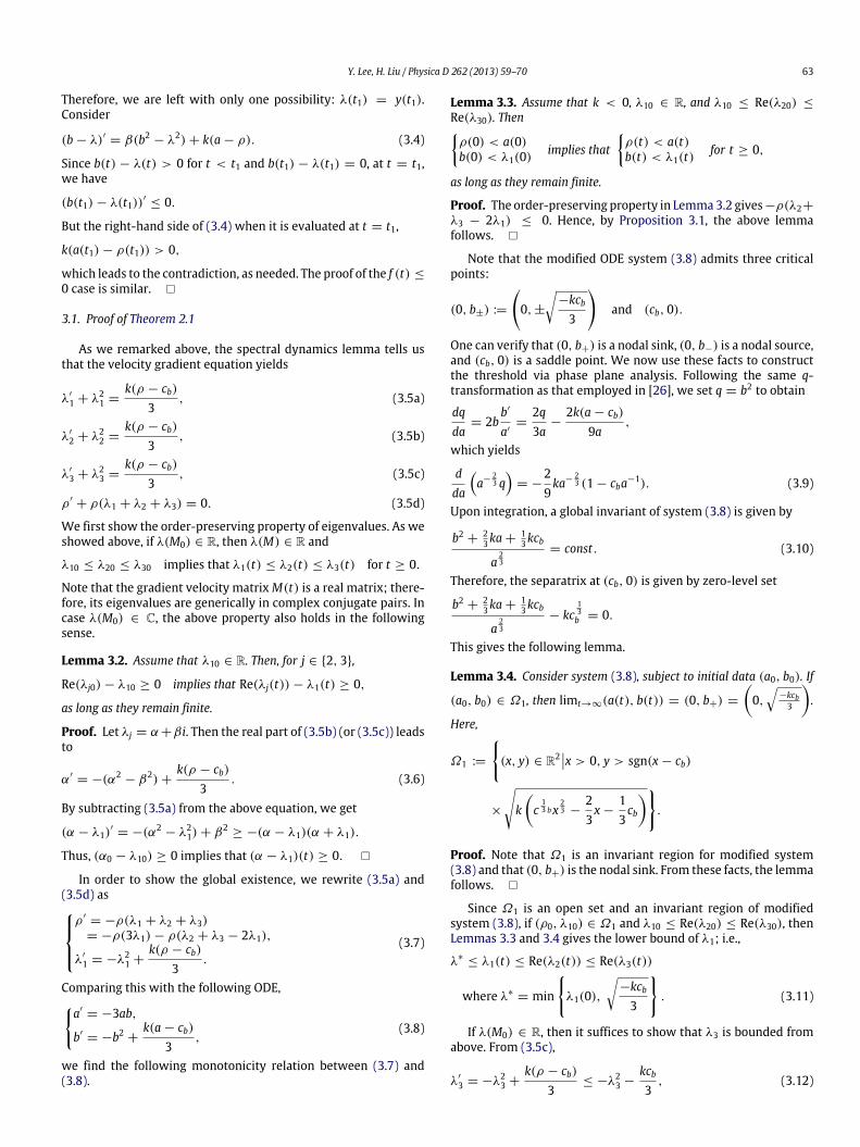
bounded solutions is very rich in phase space (ρ, λ1, λ2, λ3),which can be visualized through a qualitative diagram in thesubspace (λ1, λ3 − λ1, ρ) (Fig. 1). From the figure, one mayalso see that a critical threshold surface should lie somewherebetween the two shaded surfaces.

(iv) The condition for global regularity in Theorem 2.3 is obtainedusing only a global invariant, which is a set of measure zeroin the space of eigenvalues with ρ0 > 0. This global existenceresult, though starting from a thin initial set, when combinedwith Theorem 2.4 does suggest the existence of a criticalthreshold for the case k > 0. It would be interesting to identifya larger set of initial data than that in Theorem 2.3 for theglobal existence.

(v) For the k > 0 case, the spectral gap λ2 − λ1 as described inTheorem 2.4 plays an important role. This fact is consistentwith the known result in the 2D case (Theorem 1.2 in [27]).

(vi) The results in Theorems 2.1–2.4 may suggest the criticalthreshold phenomenon for the full Euler–Poisson equations.

For the proof of each theorem, we need the following lemma.

Lemma 2.6 (Spectral Dynamics [26, Lemma 3.1]). Consider the non-linear transport equation ut + u · ∇xu = F . Let λ := λ(∇xu)(t, x)denote an eigenvalue of ∇xu with corresponding left and right nor-

malized eigenpair, l, r = 1. Then λ is governed by the forced Riccati

equation

λ + λ2 := ∂tλ + u · ∇xλ + λ2 = l, ∇xFr.

Fig. 1. The subthreshold and the superthreshold are shaded surfaces when k < 0.

This lemma when applied to (1.3) gives

λi+ λ2

i= k

n(ρ − cb), i ∈ 1, . . . , n, (2.3a)

ρ + ρ(λ1 + · · · + λn) = 0. (2.3b)From (2.3a) it follows that(λi − λj)

= −(λi − λj)(λi + λj), i, j ∈ 1, . . . , n.This shows that, if λ(M0) ∈ R, then λ(M) ∈ R. Moreover, if λ(M0)∈ R, then the order of λini=1 is preserved in time; i.e.,If λ1(0) ≤ · · · ≤ λn(0), then λ1(t) ≤ · · · ≤ λn(t)

for t ≥ 0. (2.4)This monotonicity-preserving property remains valid in a strictsense because λi − λj = 0 as long as λi0 − λj0 = 0. Note that(2.3) is an (n + 1)-by-(n + 1) ordinary differential equation (ODE)system; when n ≥ 3, it is no longer possible to employ the precisephase plane analysis as carried out in [25] for (ux, ρ) and in [27]for (β, ρ), with β being a combined quantity of two eigenvaluesthrough a global invariant. The key argument in our proofs here isto use the order-preserving property of generic eigenvalues.

In the proof of Theorems 2.1–2.2 with k < 0, the order-pre-serving property of λ(M) together with non-negativity of thedensity enables us to obtain the following:−nρλn ≤ ρ ≤ −nρλ1.

This two-sided differential inequality leads to the desired thresh-olds for both global existence and finite-time blow up. In thepresence of complex eigenvalues, we also need the followingorder-preserving property to prove the global boundedness of theimaginary part of the eigenvalues. If λ1(0) is real andλ1(0) ≤ Re(λj(0)), then λ1(t) ≤ Re(λj(t))

for t ≥ 0, j ∈ 2, . . . , n.In the proof of Theorem 2.4 with k > 0, we use the order-pre-serving property to deduce some 2-by-2 ODE systems with con-trollable time-dependent coefficients, which when combinedwithsome comparison argument lead to the desired blow up results.

From system (2.3), it follows that

(λi − λj) = (λi0 − λj0)e−

t

0 (λi+λj) ds, i ∈ 1, 2, 3,and

ρ = ρ0e−

t

0 (λ1+λ2+λ3) ds.

These combined lead to the spectral invariant as obtained in [26];i.e.,

S(t) := (λ1 − λ2)(λ2 − λ3)(λ3 − λ1)

ρ2 = S(0). (2.5)

62 Y. Lee, H. Liu / Physica D 262 (2013) 59–70

Our results are obtained from a comparison of eigenvalues of theoriginal system to solutions of dominated systems, which implic-itly follow the order indicated by this spectral invariant; thereforeour results are consistent with (2.5). This comment also applies tothe higher-dimensional case.

We point out that, for the k < 0 case, only the density andone eigenvalue need to be controlled for proving the global exis-tence or the finite-time blow up. Hence, for the k < 0 case, thekey arguments summarized above work equally well for arbitraryn-dimensional REP equations (n > 3). For the k > 0 case, our ar-gument for solution blow up extends only to 4-dimensional REPequations. For completeness, we also state n-dimensional resultsfor the k < 0 case, the 4-dimensional blow up result, and the n-dimensional global existence result for the k > 0 case below, andwe outline some main arguments of their proofs in Section 4.

Theorem 2.7 (Extension of Theorem 2.1). Consider the nD attractive

REP system (1.3) with k < 0 and with non-zero background cb > 0.Assume that λ10 ∈ R and λ10 ≤ Re(λi0), i = 2, 3, . . . , n. Thesolution of the nD REP system remains bounded for all time if ρ0 > 0and

λ10 > sgn(ρ0 − cb)

k

c

n−2n

b

n − 2ρ

2n

0 − 2n(n − 2)

ρ0 − cb

n

.

Theorem 2.8 (Extension of Theorem 2.2). Consider the nD attractive

REP system (1.3) with k < 0 and with non-zero background cb > 0.Assume that λ(M0) ∈ R. The solution of the nD REP system will blow

up in finite time if ρ0 > 0 and

λn0 < sgn(ρ0 − cb)

k

c

n−2n

b

n − 2ρ

2n

0 − 2n(n − 2)

ρ0 − cb

n

. (2.6)

Theorem 2.9 (Extension of Theorem 2.3). Consider the nD repulsive

REP system (1.3) with k > 0 and with non-zero background cb > 0.The solution of the nD REP system remains bounded for all time if all

eigenvalues are initially real and identical.

Theorem 2.10 (Finite-Time Blow Up for 4D REP with k > 0). Con-sider the 4D repulsive REP system (1.3)with k > 0 and with non-zero

background cb > 0. Assume that λ(M0) ∈ R. The solution of the 4DREP system will blow up in finite time provided that ρ0 > 0 and

λ20 − λ10 ≥kρ0.

Remark 2.11. Two remarks are in order at this point.

(i) The bound Λn(k, ρ0) in Theorems 2.7 and 2.8 is well definedsince the quantity under the square root is non-negative:

− k

n

1n

2 − 1

c

2n

b− ρ

2n

0

2

×

n

2 −1

j=1

jc

j−1(n/2)b

ρ(n/2)−1−j

(n/2)0

≥ 0, n-even,

− k

n

1(n − 2)

c

1n

b− ρ

1n

0

2

×

(n − 2)cn−2n

b+

n−2

j=1

2jcj−1n

bρ

n−1−j

n

0

≥ 0, n-odd.

(ii) Under the assumptions of Theorem 2.8, we may use the traceofM to derive a different threshold for the finite-time blow up.In fact, taking the trace of (1.3a), we obtain

(tr(M)) + tr(M2) = k(ρ − cb),

which holds for both full Euler–Poisson equations and re-stricted Euler–Poisson equations. When λ(M) ∈ R, we have

tr(M2) ≥ 1n(tr(M))2. (2.7)

Hence the trace d = tr(M) = n

i=1 λi satisfies

d ≤ −d

2

n+ k(ρ − cb). (2.8)

This, when combined with ρ = −ρd, leads to the following blowup condition.

The solution of the nD REP system will blow up in finite time ifρ0 > 0 and

d0

n< sgn(ρ0 − cb)

k

c

n−2n

b

n − 2ρ

2n

0 − 2n(n − 2)

ρ0 − cb

n

. (2.9)

This threshold condition is slightly sharper than (2.6).We note that the same threshold condition (2.9) for finite-time

blow up is obtained in [33] for the full EP system by assuming that∇ × u0 = 0, with whichM0 is symmetric, and so isM(t) for t > 0.This ensures that λ(M) is real for all time. In contrast, for the REPsystem λ(M) remains real as long as it is real at t = 0.

3. Attractive case, k < 0

We start this section with a proposition which compares thefollowing two ODE systems:ρ = αρλ + ρf (t),

λ = βλ2 + kρ + γ(3.1)

anda = αab,

b = βb

2 + ka + γ .(3.2)

Here, α, β, γ , and k are fixed constants, and f (t) is a continuousfunction.

Proposition 3.1. Let α, k < 0.If f (t) ≥ 0, ∀t ≥ 0, then

a(0) < ρ(0)λ(0) < b(0) implies that

a(t) < ρ(t),λ(t) < b(t).

If f (t) ≤ 0, ∀t ≥ 0, thenρ(0) < a(0)b(0) < λ(0) implies that

ρ(t) < a(t),b(t) < λ(t).

Proof. This proposition can be proved by contradiction. Let f (t) ≥0, and suppose that t1 is the earliest time when the aboveproposition is violated. Then

a(t1) = a(0)e t10 αb ds

< ρ(0)e t10 αλ ds

≤ ρ(0)e t10 αλ ds

e

t10 f (s) ds

= ρ(t1). (3.3)

Y. Lee, H. Liu / Physica D 262 (2013) 59–70 63

Therefore, we are left with only one possibility: λ(t1) = y(t1).Consider

(b − λ) = β(b2 − λ2) + k(a − ρ). (3.4)

Since b(t) − λ(t) > 0 for t < t1 and b(t1) − λ(t1) = 0, at t = t1,we have

(b(t1) − λ(t1)) ≤ 0.

But the right-hand side of (3.4) when it is evaluated at t = t1,

k(a(t1) − ρ(t1)) > 0,

which leads to the contradiction, as needed. The proof of the f (t) ≤0 case is similar.

3.1. Proof of Theorem 2.1

As we remarked above, the spectral dynamics lemma tells usthat the velocity gradient equation yields

λ1 + λ2

1 = k(ρ − cb)

3, (3.5a)

λ2 + λ2

2 = k(ρ − cb)

3, (3.5b)

λ3 + λ2

3 = k(ρ − cb)

3, (3.5c)

ρ + ρ(λ1 + λ2 + λ3) = 0. (3.5d)

We first show the order-preserving property of eigenvalues. As weshowed above, if λ(M0) ∈ R, then λ(M) ∈ R and

λ10 ≤ λ20 ≤ λ30 implies that λ1(t) ≤ λ2(t) ≤ λ3(t) for t ≥ 0.

Note that the gradient velocity matrixM(t) is a real matrix; there-fore, its eigenvalues are generically in complex conjugate pairs. Incase λ(M0) ∈ C, the above property also holds in the followingsense.

Lemma 3.2. Assume that λ10 ∈ R. Then, for j ∈ 2, 3,Re(λj0) − λ10 ≥ 0 implies that Re(λj(t)) − λ1(t) ≥ 0,

as long as they remain finite.

Proof. Let λj = α+βi. Then the real part of (3.5b) (or (3.5c)) leadsto

α = −(α2 − β2) + k(ρ − cb)

3. (3.6)

By subtracting (3.5a) from the above equation, we get

(α − λ1) = −(α2 − λ2

1) + β2 ≥ −(α − λ1)(α + λ1).

Thus, (α0 − λ10) ≥ 0 implies that (α − λ1)(t) ≥ 0.

In order to show the global existence, we rewrite (3.5a) and(3.5d) as

ρ = −ρ(λ1 + λ2 + λ3)= −ρ(3λ1) − ρ(λ2 + λ3 − 2λ1),

λ1 = −λ2

1 + k(ρ − cb)

3.

(3.7)

Comparing this with the following ODE,a = −3ab,

b = −b

2 + k(a − cb)

3,

(3.8)

we find the following monotonicity relation between (3.7) and(3.8).

Lemma 3.3. Assume that k < 0, λ10 ∈ R, and λ10 ≤ Re(λ20) ≤Re(λ30). Thenρ(0) < a(0)b(0) < λ1(0)

implies that

ρ(t) < a(t)b(t) < λ1(t)

for t ≥ 0,

as long as they remain finite.

Proof. The order-preserving property in Lemma3.2 gives−ρ(λ2+λ3 − 2λ1) ≤ 0. Hence, by Proposition 3.1, the above lemmafollows.

Note that the modified ODE system (3.8) admits three criticalpoints:

(0, b±) :=

0, ±

−kcb

3

and (cb, 0).

One can verify that (0, b+) is a nodal sink, (0, b−) is a nodal source,and (cb, 0) is a saddle point. We now use these facts to constructthe threshold via phase plane analysis. Following the same q-transformation as that employed in [26], we set q = b

2 to obtain

dq

da= 2b

b

a = 2q3a

− 2k(a − cb)

9a,

which yields

d

da

a− 2

3 q

= −2

9ka

− 23 (1 − cba

−1). (3.9)

Upon integration, a global invariant of system (3.8) is given by

b2 + 2

3ka + 13kcb

a23

= const. (3.10)

Therefore, the separatrix at (cb, 0) is given by zero-level set

b2 + 2

3ka + 13kcb

a23

− kc

13b

= 0.

This gives the following lemma.

Lemma 3.4. Consider system (3.8), subject to initial data (a0, b0). If

(a0, b0) ∈ Ω1, then limt→∞(a(t), b(t)) = (0, b+) =0,

−kcb

3

.

Here,

Ω1 :=

(x, y) ∈ R2x > 0, y > sgn(x − cb)

×

k

c

13 bx

23 − 2

3x − 1

3cb

.

Proof. Note that Ω1 is an invariant region for modified system(3.8) and that (0, b+) is the nodal sink. From these facts, the lemmafollows.

Since Ω1 is an open set and an invariant region of modifiedsystem (3.8), if (ρ0, λ10) ∈ Ω1 and λ10 ≤ Re(λ20) ≤ Re(λ30), thenLemmas 3.3 and 3.4 gives the lower bound of λ1; i.e.,

λ∗ ≤ λ1(t) ≤ Re(λ2(t)) ≤ Re(λ3(t))

where λ∗ = min

λ1(0),

−kcb

3

. (3.11)

If λ(M0) ∈ R, then it suffices to show that λ3 is bounded fromabove. From (3.5c),

λ3 = −λ2

3 + k(ρ − cb)

3≤ −λ2

3 − kcb

3, (3.12)

64 Y. Lee, H. Liu / Physica D 262 (2013) 59–70

and we have

λ3 < −

λ3 +

−kcb

3

λ3 −

−kcb

3

.

Thus, λ3(t) ≤ maxλ3(0),

− kcb

3

. Together with (3.11), this

proves Theorem 2.1 when Im(λj0) = 0, j ∈ 2, 3.If Im(λj0) = 0 for some j ∈ 2, 3, then we need to bound both

α(t) := Re(λj(t)) and β(t) := Im(λj(t)). We show that there existuniform upper bounds of α(t) and |β(t)|.Lemma 3.5. Assume that λ10 ∈ R and Im(λj0) = 0. If (ρ0, λ10) ∈Ω1 and λ10 ≤ Re(λj0), then

α(t) ≤ max

Re(λj0),

Im(λj0)K ∗2 − kcb

3

and

|β(t)| ≤ |Im(λj0)|K ∗,

where K∗is a constant independent of t.

Proof. From the imaginary part of (3.5b), we have β = −2αβ .Hence

|β(t)| = |β(0)e−t

0 2α(s) ds|≤ |β(0)|e−

t

0 2λ1(s) ds, (3.13)

where the inequality comes from Lemma 3.2. Note that Ω1 is anopen set and that, given any initial data (ρ0, λ10) ∈ Ω1 for system(3.7), we can find > 0 and initial data (a(0), b(0)) := (ρ0 + ,λ10 − ) ∈ Ω1 for modified system (3.8). Therefore, by Lemma 3.3and the fact that there exists time T ∗ ≥ 0 such that b(t) > 0 for allt ≥ T

∗, we have

e−

t

0 2λ1(s) ds ≤ e−

t

0 2b(s) ds ≤ max0≤t≤T∗

e−

t

0 2b(s) ds

=: K ∗.

This gives |β(t)| ≤ |β(0)|K ∗.Also, by (3.5a) and the upper bound of |β(t)|, we have

α(t) < −α2(t) + (|β(0)|K ∗)2 − kcb

3

= −

α(t) +

(|β(0)|K ∗)2 − kcb

3

×

α(t) −

(|β(0)|K ∗)2 − kcb

3

. (3.14)

Thus, α(t) ≤ maxα(0),

(|β(0)|K ∗)2 − kcb

3

.

Together with (3.11), this completes the proof of Theorem 2.1.

3.2. Proof of Theorem 2.2

For the blow up condition, we rewrite (3.5c) and (3.5d):

ρ = −ρ(λ1 + λ2 + λ3)= −ρ(3λ3) − ρ(λ1 − λ3) − ρ(λ2 − λ3),

λ3 = −λ2

3 + k(ρ − cb)

3.

(3.15)

Similarly, we shall compare the above system with the followingmodified system:a = −3ab,

b = −b

2 + k(a − cb)

3.

(3.16)

Following a similar proof to that of Lemma 3.3, we find the mono-tonicity relation between (3.15) and (3.16).

Fig. 2. Ω1 and Ω2 for k < 0.

Lemma 3.6. Assume that λ(M0) ∈ R and λ10 ≤ λ20 ≤ λ30. Thena(0) < ρ(0)λ3(0) < b(0) implies that

a(t) < ρ(t)λ3(t) < b(t)

for t ≥ 0.

We shall prove the blow up of solutions to modified system(3.16), i.e., b(t) → −∞ in finite time, which in turn, by Lemma 3.6,implies that λ3(t) → −∞ in finite time.

Note that system (3.16) is the same as (3.8). We thus have thesame global invariant as (3.10). Hence, from the separatrix curvegiven by

b2 + 2

3ka + 13kcb

a23

− kc

13b

= 0,

we can show the blow up region of system (3.16).

Lemma 3.7. Consider the modified system (3.16), subject to initial

data (a0, b0). If (a0, b0) ∈ Ω2, then b → −∞, a → ∞ at a finite

time. Here,

Ω2 :=

(x, y) x > 0, y < sgn(x − cb)

×

k

c

13 bx

23 − 2

3x − 1

3cb

.

Proof. Note that Ω2 is an invariant region, which is decomposedas Ω l

2 ∩ Ω r

2 ∩ Ωu

2 , with

Ω l

2 := Ω2 ∩ (x, y) | x ≤ cb,Ω r

2 := Ω2 ∩ (x, y) | x > cb, y < 0and Ωu

2 := Ω2 ∩ (x, y) | x > cb, y ≥ 0 (see Fig. 2 in Sec-tion 3.1). It is straightforward to verify that, if (a0, b0) ∈ Ω l

2 ∪ Ωu

2 ,then (a(t), b(t)) ∈ Ω r

2 in finite time. Note that, if (a0, b0) ∈ Ω r

2,then a(t) is increasing in t . Thus, a(t) > cb, ∀t . This implies thatb

< −b2, which upon integration yields

b(t) <b0

tb0 + 1.

Hence, the blow up time tB of b(t) must satisfy

tB < − 1

b0.

Also a(t) approaches ∞ in finite time due to the global invariant(3.10).

Y. Lee, H. Liu / Physica D 262 (2013) 59–70 65

The last step of proving Theorem 2.2 is to combine the compar-ison principle in Lemma 3.6 with Lemma 3.7. We notice that Ω2 isan open set and that, for any given initial data (ρ0, λ30) ∈ Ω2 fororiginal system (3.15), we can always find > 0 such that the ini-tial data (ρ0 − , λ30 + ) ∈ Ω2 for modified system (3.16). Thislatter initial data will lead to finite-time blow up of the modifiedsystem and thus the initial data (ρ0, λ30) ∈ Ω2 will lead to finite-time blow up of the original system.

4. Repulsive case, k > 0

4.1. Proof of Theorem 2.3

This subsection is devoted to the proof of global existence forREP equations with k > 0. The spectral dynamics lemma tells usthat the velocity gradient equation yields

λi= −λ2

i+ k(ρ − cb)

3, i = 1, 2, 3,

ρ = −ρ(λ1 + λ2 + λ3).(4.1)

Since λ10 = λ20 = λ30, by the first equation of (4.1), we haveλ1(t) = λ2(t) = λ3(t), ∀t ≥ 0. Let λ := λi; then, by (4.1), we have

λ = −λ2 + k(ρ − cb)

3,

ρ = −3ρλ.(4.2)

To obtain a global invariant we set q := λ2; then, from (4.2) wededuce thatdq

dρ= 2λ

λ

ρ = − 23ρ

−q + k(ρ − cb)

3

.

Against the integrating factor of ρ− 23 , we have

d

dρ

ρ− 2

3 q

= −2

9kρ− 2

3 + 2kcb9

ρ− 53 .

Integrations with q = λ2 give

ρ− 23 λ2 = −2k

3ρ

13 − kcb

3ρ− 2

3 + Const

orλ2 + 2k

3 ρ + kcb

3

ρ2/3 = Const.

From this it follows that ρ is bounded from above and away fromzero, which in turn gives the boundedness of λ for all t ≥ 0. Thiscomplete the proof of Theorem 2.3.

4.2. Proof of Theorem 2.4

This section is devoted to the proof of finite-time blow up forREP equations with k > 0. From (4.1), it follows that

(λ2 − λ1) = −(λ2 − λ1)(λ2 + λ1),

(λ2 + λ1) = −λ2

1 − λ22 − 2kcb

3+ 2kρ

3.

(4.3)

Let x := λ2 − λ1, y := λ2 + λ1 and g(t) := 2k3 ρx− 3

2 . Then (4.3)becomes

x = −xy, (4.4a)

y = −y

2

2+ G(x, g(t)), (4.4b)

where we have used the following:

G(x, g(t)) := −x2

2− 2kcb

3+ g(t)x

32 .

From (4.4a), we have

x(t) = x(0)e−t

0 y(s) ds,

and hence x(t) ≡ 0 is an invariant. We thus consider only thex(0) = λ20 − λ10 > 0 case. A simple calculation gives

g(t) =

2k3

ρx− 32

= 2k3x− 3

2

ρ − 3

2x−1

xρ

= 2k3

ρx− 32

−(λ1 + λ2 + λ3) + 3

2y

= 2k3

ρx− 32

12(λ1 + λ2) − λ3

≤ 0.

Here, the last inequality comes from the order-preserving propertyof λ(M) and x(t) > 0, ∀t ≥ 0. Therefore g(t) is non-increasing intime. This fact gives the bound of g(t),

0 < g(t) ≤ g(0) = 2k3

ρ0

x3/20

.

Using the upper bound of g(t), we arrive at the following obser-vation.

Lemma 4.1. The solution of (4.4) will blow up in finite time if one of

the following two conditions is fulfilled:

(i) x0 >

k3ρ4

04cb

16,

(ii) x0 =

k3ρ4

04cb

16, y0 < 0.

Proof. Since 0 < g(t) ≤ g(0), ∀t ≥ 0, we have

G(x, g(t)) ≤ G(x, g(0)), ∀x > 0.

Also, a simple calculation gives

maxx>0

G(x, g(0)) = 16k4ρ4

0

x60

− 2kcb3

.

Therefore, from (4.4b), it follows that

y ≤ −y

2

2+ 1

6k4ρ4

0

x60

− 2kcb3

,

which gives the desired results.

Using the given initial data x0 and ρ0, we replace the time-dependent coefficient g(t) of (4.4b) by

N := g(0) = 2k3

ρ0

x032

and construct a corresponding new system. That is, finding theother blow up region of system (4.4) is carried out by comparisonwith the following system:

a = −ab,

b = −b

2

2+ G(a,N).

(4.5)

From now on, we assume that x0 <

k3ρ4

04cb

16so that the system

(4.5) has two equilibrium points (a∗i, 0), i = 1, 2, with

0 < a∗2 <

9N2

4< a

∗1.

66 Y. Lee, H. Liu / Physica D 262 (2013) 59–70

Indeed, G(a,N) has its local maximum at a = 94N

2 and G( 94N

2,N) > 0. Further calculation shows that (a∗

1, 0) is a saddle pointand (a∗

2, 0) is a spiral of ODE system (4.5).We first show the monotonicity relation between (4.4) and

(4.5).

Lemma 4.2.0 < a0 < x0y0 < b0,

implies that

a(t) < x(t)y(t) < b(t),

∀t ≥ 0,

as long as a(t) > 94N

2, ∀t ≥ 0.

Proof. It can be proved by contradiction. Suppose that t1 is theearliest time when the above lemma is violated, then

a(t1) = a0e−

t10 b(s) ds < x0e

− t10 b(s) ds < x0e

− t10 y(s) ds = x(t1).

Therefore, we are left with only one possibility: y(t1) − b(t1) = 0.From (4.4b) and the second equation of (4.5),

(b − y) = −12(b − y)(b + y) + G(a,N) − G(x, g(t)). (4.6)

At t = t1, we have

(b − y)(t1) ≤ 0.

But the right-hand side of (4.6) is positive. In fact, when it isevaluated at t = t1,

RHS = G(a(t1),N) − G(x(t1), g(t1))

≥ G(a(t1), g(t1)) − G(x(t1), g(t1))

= Gx(η, g(t1))(a(t1) − x(t1)).

The last equality comes from the mean value theorem with η ∈(a(t1), x(t1)). Also,

Gx(η, g(t1)) = η12

32g(t1) − η

12

≤ η12

32N − η

12

< 0,

since η ≥ a(t1) > 94N

2. Therefore, the right-hand side of (4.6) ispositive. This leads to a contradiction, as needed.

Nowwewant to find finite-time blow up conditions for system(4.5), which, in turn, by Lemma 4.2, imply the finite-time blow upof the original system (4.4). To this end, we set q := b

2. Then, from(4.5), we deduce that

dq

da= 2b · b

a = q

a+ a + 4kcb

3a− 2N

√a.

So,

d

da

q

a

= 1 + 4kcb

3a2− 2N√

a= − 2

a2G(a,N).

Integration leads to a global invariant:

b2

a= −2

a

c

G(a,N)

a2da, where c is some constant. (4.7)

By setting (a, b) = (a∗1, 0), we find the separatrix curve passing

(a∗1, 0),

b2

a= −2

a

a∗1

G(s,N)

s2ds. (4.8)

Fig. 3. Ω1 and Ω2 for k > 0.

The above curve has two x intercepts. One is (a∗1, 0) and the

other is denoted by (a∗, 0) with 0 < a∗ < a

∗2. In fact, consider

a∗1

a

G(s,N)

s2ds =

a∗2

a

G(s,N)

s2ds +

a∗1

a∗2

G(s,N)

s2ds.

Note that G(a,N) ≥ 0, ∀a ∈ [a∗2, a

∗1] and lima→0+

a∗2

a

G(s,N)

s2ds →

−∞. This proves the existence of intercept (a∗, 0) and thefollowing identity:

a∗1

a∗

G(s,N)

s2ds = 0. (4.9)

Together with the comparison lemma, (4.8) gives the followingresults.

Lemma 4.3. The solution of (4.4) will blow up in finite time if

(x0, y0) ∈ Ω1,

where

Ω1 :=

(x, y) | x >94N

2and

y < sgn(x − a∗1)

2x

a∗1

x

G(s,N)

s2ds

.

Proof. Since we have the comparison between two systems (4.4)and (4.5), it suffices to show the finite-time blow up of the solutionfor modified system (4.5). From (4.8), we know that Ω1 is aninvariant region, which is decomposed as Ω l

1 ∩ Ω r

1 ∩ Ωu

1 , with

Ω l

1 := Ω1 ∩(x, y)| x ≤ 9

4N

2

,

Ω r

1 := Ω1 ∩(x, y)| x >

94N

2, y < 0

,

and Ωu

1 := Ω1 ∩ (x, y)| y ≥ 0 (see Fig. 3). It is straightforward toverify that, if (a0, b0) ∈ Ω l

1 ∪ Ωu

1 , then (a(t), b(t)) ∈ Ω r

1 in finitetime. Therefore, without loss of generality, we let (a0, b0) ∈ Ω r

1,then a(t) > a

∗1 and b(t) < 0 for all t ≥ 0. This implies that

b = −b

2

2+ G(a,N) < −b

2

2,

which upon integration yields

b(t) <2b0

tb0 + 2.

Y. Lee, H. Liu / Physica D 262 (2013) 59–70 67

Hence, the blow up time tB of b(t) must satisfy

tB < − 2

b0.

Also, a(t) approaches ∞ in finite time due to the global invariantin (4.7).

The blow up condition in the above lemma was obtained bycomparison with system (4.5) as long as a(t) > 9

4N2. In the re-

gion where a(t) ≤ 94N

2, we obtain blow up results by a differentargument.

Lemma 4.4. The solution of (4.4) will blow up in finite time if

(x0, y0) ∈ Ω l

2 ∪ Ω r

2,

where

Ω l

2 := (x, y)| 0 < x < a∗, ∀y ∪ (x, y)| x = a

∗, y = 0,and

Ω r

2 :=

(x, y) ∈ R2| a∗ < x ≤ 94N

2and

y < −

2x

a∗1

x

G(s,N)

s2ds

.

Proof. In Lemma 4.1, we showed that G(x, g(t)) ≤ G(x,N), ∀x >0. This gives the following ODI.

x = −xy,

y ≤ −y

2

2+ G(x,N).

(4.10)

If (x0, y0) ∈ Ω l

2 with y0 ≥ 0, then, from x = −xy, we have

x(t) < a∗, ∀t > 0 as long as y ≥ 0. Hence

y ≤ G(x,N) ≤ G(a∗,N) < 0.

Therefore, y(t) will be negative after t∗ = − y0G(a∗,N)

.We now consider (x0, y0) ∈ Ω l

2 with y0 < 0; if x(t) ≤ a∗ for all

t > 0, we have

y ≤ −y

2

2+ G(x,N) < −y

2

2.

This leads to the finite-time blow up, unless (x(t), y(t)) enters Ω r

in finite time.In such a case with (x0, y0) ∈ Ω r

2, we deduce that

dy2

dx= 2y · y

x = −2xy ≥ −2

x

−y

2

2+ G(x,N)

.

Therefore,

d

dx

y2

x

≥ − 2

x2G(x,N).

Integration gives

y2

x− y

20

x0≥ −2

x

x0

G(s,N)

s2ds. (4.11)

Now, consider a point (x0, y∗) on separatrix curve (4.8) which isabove (x0, y0); i.e.,

y2∗x0

= −2

x0

a∗1

G(s,N)

s2ds. (4.12)

Since y20 > y

2∗ and (4.11), we obtain

y2

x+ 2

x

x0

G(s,N)

s2ds ≥ y

20

x0>

y2∗x0

= −2

x0

a∗1

G(s,N)

s2ds.

We thus have

y2

x> −2

x

a∗1

G(s,N)

s2ds. (4.13)

This relation shows that, if (x0, y0) ∈ Ω r

2, then no (x(t), y(t))crosses separatrix curve (4.8). Therefore, if (x0, y0) ∈ Ω r

2 with x0≤ a

∗2, then

(x(t), y(t)) ∈ Ω r ∩ (x, y)| x > a∗2

in finite time.It is left to consider (x0, y0) ∈ Ω r

2 ∩ (x, y)| x > a∗2. This set

ensures that ∃δ > 0 such that

y20 = δ + 2x0

a∗1

x0

G(s,N)

s2ds.

Therefore, from (4.11),

y2

x≥ y

20

x0− 2

x

x0

G(s,N)

s2ds

>δ

2x0+ 2

a∗1

x0

G(s,N)

s2ds − 2

x

x0

G(s,N)

s2ds

≥ δ

2x0+ 2

a∗1

x

G(s,N)

s2ds

≥ δ

2x0, (4.14)

where the last inequality comes from the fact that a∗2 < x0 <

x(t), ∀t > 0,

G(x,N) ≥ 0, x ∈ [a∗2, a

∗1] and G(x,N) ≤ 0, x ∈ [a∗

1, ∞].By substituting the inequality in (4.14) into the first equation in(4.10), we obtain

x = −xy

≥ x32

δ

2x0, δ > 0. (4.15)

Therefore, x(t) → ∞ in finite time. This gives the desired re-sult.

By combining the blowup conditions in Lemmas 3.3 and 3.4, wecan get the following blow up condition. Either

0 < x0 < a∗ (4.16)

or

x0 ≥ a∗ with y0 < sgn(x0 − a

∗1)

×

x20 +

a∗1 + 4kcb

a∗1

x0 − 4Nx

320 − 4kcb

3. (4.17)

The last step of proving Theorem 2.4 is to convert the blow upconditions in (4.16) and (4.17) into conditions which involve theoriginal variables ρ0 and λi.

Let β := a∗1

x0. Since G(x,N) = − x

2

2 − 2kcb3 + Nx

32 and G(a∗

i,N) =

0, i = 1, 2, we have

− (βx0)2

2− 2kcb

3+ 2kρ0

3x3/20

(βx0)32 = 0.

68 Y. Lee, H. Liu / Physica D 262 (2013) 59–70

This is equivalent to

34kcb

x20 = − 1

β2 + ρ0

cb

· 1√β

. (4.18)

Also, let α := a∗

x0. Since the separatrix curve (4.8) passes through

(a∗, 0), we have

0 =a∗ − 4kcb

3a∗ − 4N√a∗

−

a∗1 − 4kcb

3a∗1

− 4Na∗1

=

αx0 − 4kcb3αx0

− 8kρ0

3x3/20

√αx0

−

βx0 − 4kcb3βx0

− 8kρ0

3x3/20

βx0

, (4.19)

or

(α − β)x20 − 4kcb3

1α

− 1β

− 8kρ0

3

√α −

β

= 0.

This is equivalent to

34kcb

x20 = − 1

αβ+ 2ρ0

cb

1√α + √

β. (4.20)

With α, β introduced above, the blow up conditions in (4.16) and(4.17) can be written as

α > 1

and

α ≤ 1 with λ20 + λ10 < sgn(1 − β)

×

(β + 1)(λ20 − λ10)2 − 4k3

2ρ0 + cb − 3cb

β

,

respectively. This, together with Lemma 4.1, completes the proofof Theorem 2.4.

5. Extension to n dimensions

In this section, we outline the proofs of the n-dimensionaltheorems. We also prove the 4-dimensional theorem for the k > 0case.

Proof of Theorem 2.7. From (2.3b) it follows that

ρ = −ρ

n

i=1

λi

= −nρλ1 − ρ

n

i=2

λi − (n − 1)λ1

= −nρλ1 − ρ

n

i=2

Re(λi) − (n − 1)λ1

. (5.1)

Consider anyλj, j ∈ 2, . . . , n. Ifλj ∈ R, then the order-preservingproperty of real eigenvalues gives λj − λ1 ≥ 0. If Im(λj) = 0, thenLemma 3.2 implies that Re(λj) − λ1 ≥ 0. Thus,

−ρ

n

i=2

Re(λi) − (n − 1)λ1

≤ 0.

Therefore, ODE system

ρ = −nρλ1 − ρ

n

i=2

Re(λi) − (n − 1)λ1

,

λ1 = −λ2

1 + k(ρ − cb)

n,

can be compared witha = −nab,

b = −b

2 + k(a − cb)

n.

(5.2)

This gives

db2

da= 2b2

na− 2k

n2 + 2kcbn2a

;

that is,

d

da

a− 2

n b2

= −2kn2 a

− 2n + 2kcb

n2 a−1− 2

n .

Upon integration, the separatrix passing through (cb, 0) is obtainedand expressed by

b2 = k

c

n−2n

ba

2n

n − 2− 2a

n(n − 2)− cb

n

. (5.3)

Using (5.3), define an invariant region of (5.2) by

Ω 1 =

(x, y) | x > 0, y > sgn(x − cb)

×

k

c

n−2n

bx

2n

n − 2− 2x

n(n − 2)− cb

n

.

Since Ω 1 is an open set and an invariant region of system (5.2), for

any given (ρ0, λ10) ∈ Ω 1, we can always find > 0 and initial data

(a(0), b(0)) := (ρ0 + , λ10 − ) ∈ Ω 1 for system (5.2). Therefore,

Proposition 3.1 gives

λ∗ ≤ λ1(t) ≤ Re(λ2(t)) ≤ · · · ≤ Re(λn(t)),

where λ∗ := min

λ1(0),

−kcb

n

.

We now turn to finding an upper bound of maxiRe(λi(t)) andmaxi|Im(λi(t))|. For any j ∈ 1, . . . , n, let α = Re(λj) andβ = Im(λj). Then, by (3.5),

α = −α2 + β2 + k

n(ρ − cb).

If β(0) = 0, then β(t) = 0, and

α ≤ −α2 − kcb

n= −

α +

−kcb

n

α −

−kcb

n

.

This gives λj(t) ≤ maxλj0,

− kcb

n

.

If β(0) = 0, then Lemma 3.5 gives the upper bounds ofα(t) and|β(t)|.

Therefore, we complete the proof of Theorem 2.7.

Proof of Theorem 2.8. From (2.3b),

ρ = −ρ

n

i=1

λi

= −nρλn − ρ

n−1

i=1

λi + (1 − n)λn

. (5.4)

Y. Lee, H. Liu / Physica D 262 (2013) 59–70 69

The order-preserving property of real eigenvalues gives

−ρ

n−1

i=1

λi + (1 − n)λn

≥ 0.

Therefore, ODE system

ρ = −nρλn − ρ

n−1

i=1

λi + (1 − n)λn

,

λn

= −λ2n+ k(ρ − cb)

n,

(5.5)

can be compared with the same system in (5.2). Using the globalinvariant in (5.3), we define the blow up region of (5.2) by

Ω 2 =

(x, y) | x > 0, y < sgn(x − cb)

×

k

c

n−2n

bx

2n

n − 2− 2x

n(n − 2)− cb

n

.

For any given initial data (ρ0, λn0) ∈ Ω 2 for original system (5.5),

we can find > 0 such that the initial data (a(0), b(0)) := (ρ0−,λn0 + ) ∈ Ω

2 for system (5.2). We know that a(t) → ∞ andb(t) → −∞ at a finite time. Therefore, by Proposition 3.1, theinitial data (ρ0, λn0) ∈ Ω

2 will lead to finite-time blow up of theoriginal system.

Proof of Theorem 2.9. Since λ10 = λ20 = · · · = λn0, we haveλ1(t) = λ2(t) = · · · = λn(t), ∀ t ≥ 0. Let λ := λi. Then (2.3) leadsto

λ = −λ2 + k(ρ − cb)

n,

ρ = −nρλ.(5.6)

Using the same q = λ2 transform as employed in the proof ofTheorem 2.3 gives the following global invariant:

λ2 + 2kn(n−2)ρ + kcb

n

ρ2n

= Const.

This ensures the boundedness of both λ and ρ, hence completingthe proof of Theorem 2.9.

Proof of Theorem 2.10. Let x := λ2 − λ1 and y := λ2 + λ1. Then(2.3) leads to

x = −xy,

y = −y

2

2− x

2

2+ kρ

2− kcb

2.

(5.7)

Suppose that x0 = λ20 − λ10 > 0. Then x(t) = 0, ∀t ≥ 0, and thesecond equation of (5.7) leads to

y = −y

2

2+

kρ

x2− 1

x2

2− kcb

2.

From kρ0x20

− 1 ≤ 0, we can show that kρ

x2− 1 ≤ 0, ∀t ≥ 0. In fact,

kρ

x2− 1

= k

ρ

x2− 2 · ρ

x3· x

= kρ

x2−(λ1 + λ2 + λ3 + λ4) + 2y

= kρ

x2(λ1 + λ2) − (λ3 + λ4)

≤ 0.

Therefore,

y ≤ −y

2

2− kcb

2< −y

2

2,

which ensures a finite-time blow up for any y0 ∈ R. This provesTheorem 2.10.

Acknowledgments

The authors thank the reviewers, who provided valuable com-ments resulting in improvements in this paper. This research wassupported by the National Science Foundation under Grant DMS09-07963.

References

[1] P.A. Markowich, C. Ringhofer, C. Schmeiser, Semiconductor Equations,Springer-Verlag, Berlin, Heidelberg, New York, 1990.

[2] J.D. Jackson, Classical Electrodynamics, second ed., Wiley, New York, 1975.[3] U. Brauer, A. Rendall, O. Reula, The cosmic no-hair theorem and the non-linear

stability of homogeneous Newtonian cosmological models, Classical QuantumGravity 11 (9) (1994) 2283–2296.

[4] D. Holm, S.F. Johnson, K.E. Lonngren, Expansion of a cold ion cloud, Appl. Phys.Lett. 38 (1981) 519–521.

[5] T. Makino, On a local existence theorem for the evolution equation of gaseousstars, in: Patterns and Waves, in: Stud. Math. Appl., vol. 18, North-Holland,Amsterdam, 1986, pp. 459–479.

[6] M.P. Brenner, T.P. Witelski, On spherically symmetric gravitational collapse,J. Stat. Phys. 93 (3–4) (1998) 863–899.

[7] Y. Deng, T.-P. Liu, T. Yang, Z. Yao, Solutions of Euler–Poisson equations forgaseous stars, Arch. Ration. Mech. Anal. 164 (3) (2002) 261–285.

[8] I.M. Gamba, Stationary transonic solutions of a one-dimensional hydrody-namicmodel for semiconductors, Comm. Partial Differential Equations 17 (34)(1992) 553–577.

[9] P. Degond, P. Markowich, A steady state potential flowmodel for semiconduc-tors, Ann. Mat. Pura Appl. 165 (4) (1993) 87–98.

[10] T. Luo, J. Smoller, Rotating fluids with self-gravitation in bounded domains,Arch. Ration. Mech. Anal. 173 (3) (2004) 345–377.

[11] T. Luo, J. Smoller, Nonlinear dynamical stability of newtonian rotating andnon-rotating white dwarfs and rotating supermassive stars, Commun. Math. Phys.284 (2008) 425–457.

[12] G. Rein, Non-linear stability of gaseous stars, Arch. Ration. Mech. Anal. 168 (2)(2003) 115–130.

[13] G.-Q. Chen, D. Wang, Convergence of shock capturing scheme for thecompressible Euler–Poisson equations, Comm. Math. Phys. 179 (1996)333–364.

[14] Bo Zhang, Global existence and asymptotic stability to the full 1D hydrody-namic model for semiconductor devices, Indiana Univ. Math. J. 44 (3) (1995)971–1005.

[15] P. Marcati, R. Natalini, Weak solutions to a hydrodynamic model forsemiconductors and relaxation to the drift–diffusion equation, Arch. Ration.Mech. Anal. 129 (2) (1995) 129–145.

[16] F. Poupaud, M. Rascle, J.-P. Vila, Global solutions to the isothermalEuler–Poisson system with arbitrarily large data, J. Differential Equations 123(1) (1995) 93–121.

[17] D. Wang, Global solutions and relaxation limits of Euler–Poisson equations, Z.Angew. Math. Phys. 52 (4) (2001) 620–630.

[18] D.Wang, G.-Q. Chen, Formation of singularities in compressible Euler–Poissonfluidswith heat diffusion and damping relaxation, J. Differential Equations 144(1) (1998) 44–65.

[19] T. Luo, R. Natalini, Z.P. Xin, Large time behavior of the solutions to ahydrodynamic model for semiconductors, SIAM J. Appl. Math. 59 (3) (1999)810–830.

[20] Y. Guo, Smooth irrotational flows in the large to the Euler–Poisson system inR3+1, Comm. Math. Phys. 195 (1998) 249–265.

[21] S. Cordier, E. Grenier, Quasi-neutral limit of an Euler–Poisson system arisingfrom plasma physics, Comm. Partial Differential Equations 25 (5–6) (2000)1099–1113.

[22] B. Perthame, Non-existence of global solutions to Euler–Poisson equations forrepulsive forces, Japan J. Appl. Math. 7 (2) (1990) 363–367.

[23] T. Makino, Blowing up solutions of the Euler–Poisson equation for theevolution of gaseous stars. in: Proceedings of the Fourth InternationalWorkshop on Mathematical Aspects of Fluid and Plasma Dynamics, Kyoto,1991, vol. 21, 1992, pp. 615–624.

70 Y. Lee, H. Liu / Physica D 262 (2013) 59–70

[24] T. Makino, B. Perthame, Sur les solutions á symétrie sphérique de l’equationd’Euler–Poisson pour l’evolution d’etoiles gazeuses, Japan J. Appl. Math. 7 (1)(1990) 165–170.

[25] S. Engelberg, H. Liu, E. Tadmor, Critical thresholds in Euler–Poisson equations,Indiana Univ. Math. J. 50 (2001) 109–157.

[26] H. Liu, E. Tadmor, Spectral dynamics of the velocity gradient field in restrictedfluid flows, Comm. Math. Phys. 228 (2002) 435–466.

[27] H. Liu, E. Tadmor, Critical thresholds in 2-D restricted Euler–Poisson equations,SIAM J. Appl. Math. 63 (6) (2003) 1889–1910.

[28] H. Liu, E. Tadmor, Rotation prevents finite-time breakdown, Physica D 188(3–4) (2004) 262–276.

[29] H. Liu, E. Tadmor, D.Wei, Global regularity of the 4D restricted Euler equations,Physica D 239 (2010) 1225–1231.

[30] P. Vieillefosse, Local interaction between vorticity and shear in a perfectincompressible flow, J. Physique 43 (1982) 837–842.

[31] E. Tadmor, D. Wei, On the global regularity of subcritical Euler–Poissonequations with pressure, J. Eur. Math. Soc. (JEMS) 10 (3) (2008) 757–769.

[32] D. Chae, E. Tadmor, On the finite time blow up of the Euler–Poisson equationsin RN , Commun. Math. Sci. 6 (2008) 785–789.

[33] B. Cheng, E. Tadmor, An improved local blow up condition for Euler–Poissonequations with attractive forcing, Physica D 238 (2009) 2062–2066.